Domain wall motion in magnetic nanowires: An asymptotic approach

Abstract

We develop a systematic asymptotic description for domain wall motion in one-dimensional magnetic nanowires under the influence of small applied magnetic fields and currents and small material anisotropy. The magnetization dynamics, as governed by the Landau–Lifshitz–Gilbert equation, is investigated via a perturbation expansion. We compute leading-order behaviour, propagation velocities, and first-order corrections of both travelling waves and oscillatory solutions, and find bifurcations between these two types of solutions. This treatment provides a sound mathematical foundation for numerous results in the literature obtained through more ad hoc arguments.

1 Introduction

The last two decades have witnessed a revolution in micromagnetics, both in fundamental science and technology. It has long been understood that ferromagnetic domains can be controlled through external magnetic fields (Hubert and Schäfer 1998). More recent is the discovery of a new mechanism for domain wall dynamics through the interaction of magnetization and spin-polarized currents (Berger 1978, 1984 and 1996; Slonczewski 1996). The ability to change (write) magnetic domains through the application of electrical current has led to new designs of magnetic memory. One of the most spectacular realizations is the so-called race-track memory (Parkin et al. 2008; Hayashi et al. 2008), a device with a fully three-dimensional geometry comprised of an array of parallel nanowires on which domains (bits) may be read, transported, and written by applying currents.

The dynamics of magnetic domain walls in ferromagnetic nanowires under applied magnetic fields and electric current is one of the most important problems in micromagnetics and spintronics. This problem has been extensively studied experimentally (e.g. Yamaguchi et al. 2004, Beach et al. 2005 and 2006; Hayashi et al. 2007a and 2007b) and through numerical simulations (e.g. Hertel and Kirschner 2004; Weiser et al. 2010).

There have also been numerous theoretical studies of these phenomena based on the Landau-Lifshitz-Gilbert (LLG) equation. The analysis is often simplified by taking the nanowire to be one dimensional, although even in one dimension, exact solutions of the LLG equation are available only in special cases (Schryer and Walker 1974; Goussev et al 2010). A successful approach, introduced in this context by Schryer and Walker (1974) and generalised in Malozemoff and Slonczewski (1979), is to make the ansatz that under applied fields and currents, the static domain wall profile is preserved up to parameters describing its position, orientation and scale. The dynamics of these parameters is prescribed so as to try to satisfy the LLG equation as nearly as possible.

This approach has had numerous applications to domain wall motion in various regimes, and the results agree well with both numerical simulations and experiments (see, e.g., Thiaville et al. 2005; Mougin et al. 2007; Bryan et al. 2008; Yang et al. 2008; Wang et al. 2009a and 2009b; Lu & Wang 2010; Tretiakov & Abanov 2010; Tretiakov et al. 2012). However, from a mathematical point of view, this approach is ad hoc, and difficult to justify; the approximation is uncontrolled, and it is unclear how to obtain corrections to it.

Here we introduce a new approach to domain wall dynamics in thin nanowires. We develop a systematic asymptotic expansion, regarding the applied field, material anisotropy and applied current as small parameters. We derive formulas for two different types of solutions of the LLG equations, namely travelling waves and oscillating solutions, and obtain expressions for their principal characteristics, including velocity of propagation and frequency of oscillation. In particular parameter regimes, these expressions agree with results obtained in previous studies, and put them on a sound mathematical foundation; in this setting, they arise as solvability conditions for a system of inhomogeneous linear ODEs. We also obtain formulae for higher-order corrections, and carry out a systematic bifurcation analysis, including the values of applied fields and currents at which travelling-wave solutions break down, as well as bifurcations between one and two travelling waves, which arise through competition between the transverse magnetic field and material anisotropy.

1.1 Mathematical formulation

The dynamics of magnetic domain walls (DWs) in thin ferromagnetic nanowires is governed by the Landau–Lifshitz–Gilbert (LLG) equations. We use the following dimensionless form of the equations (see Thiaville et al. 2005), which includes spin-transfer torque terms:

$${\hat{\mathbf{m}}}_{t}+\alpha\hat{\mathbf{m}}\times{\hat{\mathbf{m}}}_{t}=(1+\alpha^{2})\hat{\mathbf{m}}\times\mathbf{H}(\hat{\mathbf{m}})+J{\hat{\mathbf{m}}}_{x}+\beta J{\bf\hat{m}}\times{\hat{\mathbf{m}}}_{x},$$ (1)

where $\hat{\mathbf{m}}(x,t)$ is the magnetization (a unit-vector field depending only on the coordinate along the wire $x$ and time $t$), $\alpha$ is the Gilbert damping parameter, $\beta$ the nonadiabatic spin transfer parameter, $\mathbf{H}(\hat{\mathbf{m}})$ the effective magnetic field and $J$ the applied current along the wire. The effective field, $\mathbf{H}(\hat{\mathbf{m}})$, is given by

$$\mathbf{H}=A\hat{\mathbf{m}}_{xx}+K_{1}(\hat{\mathbf{m}}\cdot\hat{\mathbf{e}}_{x})\hat{\mathbf{e}}_{x}-K_{2}(\hat{\mathbf{m}}\cdot\hat{\mathbf{e}}_{y})\hat{\mathbf{e}}_{y}+\mathbf{H}_{a},$$ (2)

where $A$ is the exchange constant, $K_{1}$ is the easy-axis anisotropy constant, $K_{2}\geq 0$ is the hard-axis anisotropy constant, and $\mathbf{H}_{a}=H_{1}\hat{\mathbf{e}}_{x}+H_{2}\hat{\mathbf{e}}_{y}+H_{3}\hat{\mathbf{e}}_{z}$ is a uniform applied field. Without loss of generality, for the rest of the paper we take $A=K_{1}=1$. Since we are interested in DW dynamics, we impose the following boundary conditions, assuming that $\mathbf{m}_{t}\to 0$ and $\mathbf{m}_{x}\to 0$ as $|x|\to\infty$:

$$\mathbf{m}(x)\times(K_{1}(\hat{\mathbf{m}}(x)\cdot\hat{\mathbf{e}}_{x})\hat{\mathbf{e}}_{x}-K_{2}(\hat{\mathbf{m}}(x)\cdot\hat{\mathbf{e}}_{y})\hat{\mathbf{e}}_{y}+\mathbf{H}_{a})\to 0,\quad\text{ as }|x|\to\infty.$$ (3)

For definiteness, we consider boundary conditions supporting “tail-to-tail” domain walls, for which

$$\lim_{x\rightarrow-\infty}\hat{\mathbf{m}}(x)\cdot\hat{\mathbf{e}}_{x}<0,\quad\lim_{x\rightarrow\infty}\hat{\mathbf{m}}(x)\cdot\hat{\mathbf{e}}_{x}>0$$ (4)

(“head-to-head” domain walls may be treated similarly).

Using polar angles $\theta(x,t)$ and $\varphi(x,t)$, we express the magnetization as $\hat{\mathbf{m}}=(\cos\theta,\sin\theta\cos\varphi,\sin\theta\sin\varphi)$ and represent (1) as a system of two PDEs

$$\alpha{\theta}_{t}+\sin\theta\varphi_{t} =(1+\alpha^{2})F_{1},$$ (5)

$$-{\theta}_{t}+\alpha{\varphi_{t}}\sin\theta =(1+\alpha^{2})F_{2},$$ (6)

where $F_{1}$ and $F_{2}$ are given as

$$F_{1}=\theta_{xx}-\tfrac{1}{2}(1+\varphi_{x}^{2})\sin 2\theta-\tfrac{1}{2}K_{2}\cos^{2}\varphi\sin 2\theta+(1+\alpha^{2})^{-1}\left(J\varphi_{x}\sin\theta+\beta J\theta_{x}\right)\\ -H_{1}\sin\theta+H_{2}\cos\theta\cos\varphi+H_{3}\cos\theta\sin\varphi,$$ (7)

$$F_{2}=\varphi_{xx}\sin\theta+2\theta_{x}\varphi_{x}\cos\theta+\tfrac{1}{2}K_{2}\sin\theta\sin 2\varphi+(1+\alpha^{2})^{-1}(\beta J\varphi_{x}\sin\theta-J\theta_{x})\\ -H_{2}\sin\varphi+H_{3}\cos\varphi.$$ (8)

We look for solutions of equations (1) depending on parameters $K_{2}$, $J$, $\mathbf{H}_{a}$, $\alpha$, and $\beta$. While, in general, this problem may not be solvable with currently available PDE techniques, substantial progress can be made in understanding the persistent or long-time behaviour by taking the some of the parameters – namely $\mathbf{H}_{a}$, $K_{2}$ and $J$ – to be small, and using the method of perturbation expansions.

2 Asymptotic analysis

We introduce a parameter ${\epsilon}\ll 1$ and set $\mathbf{H}_{a}=\epsilon\mathbf{h}_{a}=(\epsilon h_{1},\epsilon h_{2},\epsilon h_{3})$, $K_{2}=\epsilon k_{2}$, and $J=\epsilon j$. In order to capture the long-time behaviour of the problem (1), we rescale time, defining $\tau=\epsilon t$. It is straightforward to check that boundary conditions (3)–(4) for $\hat{\mathbf{m}}(x,t)$ become

$$\hat{\mathbf{m}}(\pm\infty,\tau)=(\pm 1,{\epsilon}h_{2},{\epsilon}h_{3})+O({\epsilon}^{2})$$ (9)

We seek solutions in the form of a regular perturbation expansion depending on $x$ and $\tau$ only:

$$\theta(x,t) =\theta_{0}(x,\tau)+\epsilon\theta_{1}(x,\tau)+\ldots,$$ (10)

$$\varphi(x,t) =\varphi_{0}(x,\tau)+\epsilon\varphi_{1}(x,\tau)+\ldots.$$ (11)

Substituting this expansion into the equations (1), we obtain the following system of equations, to the leading order in $\epsilon$,

$$\theta_{0,xx}-\tfrac{1}{2}(1+\varphi_{0,x}^{2})\sin 2\theta_{0} =0,$$ (12)

$$\left(\varphi_{0,x}\sin^{2}\theta_{0}\right)_{x} =0.$$ (13)

The only physical (finite micromagnetic energy) solution of (13) consistent with the boundary conditions (9) is $\varphi_{0}(x,\tau)=\varphi_{0}(\tau)$. Equation (12) then reduces to

$$\theta_{0,xx}=\tfrac{1}{2}\sin 2\theta_{0},$$ (14)

which (along with the restriction imposed by the boundary conditions) has a unique solution, given by the well known optimal DW profile

$$\theta_{0}(x,\tau)=2\arctan e^{-(x-x_{*}(\tau))},$$ (15)

as studied by Schryer and Walker (1974) and Goussev et al. (2010). Here $x_{*}(\tau)$ is a function representing the time-dependent position of the DW centre. Defining a moving coordinate $\xi=x-x_{*}(\tau)$, we see that $\theta_{0}(x,\tau)$ now depends on $x$ and $\tau$ only through $\xi$, which allows us to rewrite our original perturbation expansion as

$$\theta(x,t) =\theta_{0}(\xi)+\epsilon\theta_{1}(\xi,\tau)+\ldots,$$ (16)

$$\varphi(x,t) =\varphi_{0}(\tau)+\epsilon\varphi_{1}(\xi,t)+\ldots.$$ (17)

We now focus on the functions $x_{*}(\tau)$ and $\varphi_{0}(\tau)$, which, to the leading order in $\epsilon$, describe the time-dependent position and orientation of the DW, respectively. In what follows, we use the prime “$\;{}^{\prime}\;\,$” to denote differentiation with respect to $\xi$, and the dot “$\;\dot{}\;\>$” to denote differentiation with respect to $\tau$.

In order to determine the leading-order dynamics of the DW, we must examine the LLG equations to the first order in $\epsilon$. To this end, it is convenient to introduce new variables

$$\Theta_{1} :=\theta_{1}-(h_{2}\cos\varphi_{0}+h_{3}\sin\varphi_{0})\cos\theta_{0},$$

$$u :=\varphi_{1}\sin\theta_{0}+h_{2}\sin\varphi_{0}-h_{3}\cos\varphi_{0},$$ (18)

which vanish at infinity due to the boundary conditions (9). (One way to motivate this transformation is through the Möbius transformation which maps the boundary values for $\mathbf{h}_{a}\neq 0$ into the boundary values for $\mathbf{h}_{a}=0$.) Investigating ${\epsilon}$-order equations for $\theta_{1}$ and $\varphi_{1}$, we obtain the following system of linear equations for $\Theta_{1}$ and $u$:

$$L\Theta_{1} =f(\xi,\tau),$$ (19)

$$Lu =g(\xi,\tau),$$ (20)

where $L$ is a self-adjoint linear differential operator defined as

$$L:=-\frac{\partial^{2}}{\partial\xi^{2}}+\frac{\theta_{0}^{\prime\prime\prime}}{\theta_{0}^{\prime}},$$ (21)

and $f$ and $g$ are given by

$${f} ={(1+\alpha^{2})}^{-1}\sin\theta_{0}\left[-\alpha\dot{x}_{*}-\dot{\varphi}_{0}-\beta j\right]-h_{1}\sin\theta_{0}-\tfrac{1}{2}k_{2}\cos^{2}\varphi_{0}\sin 2\theta_{0},$$ (22)

$${g} ={(1+\alpha^{2})}^{-1}\sin\theta_{0}\left[\dot{x}_{*}-\alpha\dot{\varphi}_{0}+j\right]+\tfrac{1}{2}k_{2}\sin\theta_{0}\sin 2\varphi_{0}$$

$$\qquad\qquad\qquad\qquad\qquad{}+(1-\cos 2\theta_{0})(h_{2}\sin\varphi_{0}+h_{3}\cos\varphi_{0}).$$ (23)

A necessary condition for an equation of the form $Ly=F$, where $L$ is self-adjoint on $L^{2}(\mathbb{R})$, to have a solution is that $F$ must be orthogonal to the kernel of $L$. The kernel of the operator $L$, defined by equation (21), consists of the single element $\theta_{0}^{\prime}$. The required solvability conditions for the system (19), (20) are then

$$\left<\theta_{0}^{\prime},f\right>=0,\quad\left<\theta_{0}^{\prime},g\right>=0,$$ (24)

where angled brackets denote the $L^{2}$ inner product. Noting that $\theta_{0}^{\prime}=-\sin\theta_{0}$ and $\theta_{0}^{\prime\prime}=\tfrac{1}{2}\sin 2\theta_{0}$, it is straightforward to establish that $\left<\theta_{0}^{\prime},\theta_{0}^{\prime}\right>=2$, $\left<\theta_{0}^{\prime},\theta_{0}^{\prime\prime}\right>=0$, $\left<\theta_{0}^{\prime},\cos\theta_{0}\right>=0$ and $\left<\theta_{0}^{\prime},1\right>=-\pi$. Using these results to evaluate the inner products in (24), we find

$$\left<\theta_{0}^{\prime},f\right>=2\left[h_{1}+(1+\alpha^{2})^{-1}(\alpha\dot{x}_{*}+\dot{\varphi}_{0}+\beta j)\right]=0$$ (25)

and

$$\left<\theta_{0}^{\prime},g\right>=-k_{2}\sin 2\varphi_{0}+\pi h_{2}\sin\varphi_{0}-\pi h_{3}\cos\varphi_{0}\\ +2(1+\alpha^{2})^{-1}(\alpha\dot{\varphi}_{0}-\dot{x}_{*}-j)=0.$$ (26)

These equations lead to a system of two coupled ODEs for $\varphi_{0}$ and $x_{*}$:

$$\dot{\varphi}_{0} =\mu(h_{1},j)-\alpha\Gamma(\varphi_{0};h_{2},h_{3},k_{2}),$$ (27)

$$\dot{x}_{*} =\nu(h_{1},j)+\Gamma(\varphi_{0};h_{2},h_{3},k_{2}),$$ (28)

where

$$\Gamma =\frac{\pi}{2}\left(h_{2}\sin\varphi_{0}-h_{3}\cos\varphi_{0}\right)-\frac{k_{2}}{2}\sin 2\varphi_{0},$$ (29)

$$\mu =-h_{1}-(1+\alpha^{2})^{-1}(\beta-\alpha)j,$$ (30)

$$\nu =-\alpha h_{1}-(1+\alpha^{2})^{-1}(1+\alpha\beta)j.$$ (31)

Equations (27) and (28) determine the leading-order dynamics of the orientation and position of a DW. Considering $\mathbf{h}_{a}$, $k_{2}$ and $j$ as parameters, we will use these equations extensively throughout the rest of the paper in order to characterize the behaviour of solutions in different parameter regimes.

2.1 First-Order Correction Terms

The correction terms $\theta_{1}$ and $\varphi_{1}$ can be computed by solving equations (19) and (20). The latter, in view of the solvability conditions given by equations (27) and (28), reduce to

$$L\Theta_{1}=-\tfrac{1}{2}k_{2}\cos^{2}\varphi_{0}\sin 2\theta_{0},$$ (32)

$$Lu=\left(h_{2}\sin\varphi_{0}-h_{3}\cos\varphi_{0}\right)\left({\tfrac{\pi}{2}}\sin\theta_{0}+\cos 2\theta_{0}-1\right).$$ (33)

We have already found one solution to the homogeneous problem $Ly=0$, given by $y_{1}=\theta_{0}^{\prime}$. Now, taking into account that $\theta_{0}^{\prime}=-\operatorname{sech}\xi$, we construct the Wronskian to obtain another linearly independent solution, $y_{2}=\xi\operatorname{sech}\xi+\sinh\xi$. (Note that $y_{2}$, unlike $y_{1}$, diverges at infinity.) For $F$ square-integrable, the general square-integrable solution of the inhomogeneous equation $Ly=F$ is given by

$$y(\xi)=\tfrac{1}{2}\left(\int_{0}^{\xi}y_{2}(\eta)F(\eta)\,d\eta+a\right)y_{1}(\xi)-\tfrac{1}{2}\left(\int_{-\infty}^{\xi}y_{1}(\eta)F(\eta)\,d\eta\right)y_{2}(\xi),$$ (34)

where $a$ is an undetermined constant. Noting that $\sin\theta_{0}=\operatorname{sech}\xi$ and $\cos\theta_{0}=\tanh\xi$, it is straightforward to use (34) to obtain

$$\Theta_{1} =-\tfrac{1}{2}k_{2}\cos^{2}\varphi_{0}\xi\operatorname{sech}\xi+a(\tau)\operatorname{sech}\xi,$$ (35)

$$u =(h_{2}\sin\varphi_{0}-h_{3}\cos\varphi_{0})\tilde{u}+b(\tau)\operatorname{sech}\xi,$$ (36)

where

$$\tilde{u}=-\tfrac{1}{2}\operatorname{sech}\xi\int_{0}^{\xi}\eta\operatorname{sech}\eta\,\,\mathrm{d}\eta+\tfrac{1}{2}-{\tfrac{\pi}{4}}\sinh\xi\tanh\xi\\ +\left(\xi\operatorname{sech}\xi+\sinh\xi\right)\arctan\left(\tanh\left(\tfrac{\xi}{2}\right)\right),$$ (37)

and the functions $a(\tau)$ and $b(\tau)$ may be determined at second order in $\epsilon$. (The integral term in (37) can be expressed in terms of polylogarithm functions, but the explicit closed-form expression is omitted).

3 Domain wall dynamics

We now turn our attention to solving the equations of motion (27) and (28) for the orientation, $\varphi_{0}(\tau)$, and position, $x_{*}(\tau)$, of a DW. Firstly, from the form of the equations, it is simple to notice that the DW velocity $\dot{x}_{*}$ is given as a function of $\varphi_{0}$ and the parameters $\mathbf{h}_{a},j$ and $k_{2}$. It is therefore sufficient to first consider only equation (27) and solve it for $\varphi_{0}(\tau)$. The DW position, $x_{*}(\tau)$, can then be found by integration of (28), given the result for $\varphi_{0}(\tau)$. For what follows, it is convenient to rewrite equation (27) as

$$\dot{\varphi}_{0}=F(\varphi_{0}),$$ (38)

where the function $F$, defined as

$$F:=\mu-\alpha\Gamma,$$ (39)

depends, parametrically, on $h_{1}$, $h_{2}$, $h_{3}$, $j$ and $k_{2}$. Here, $\Gamma$ and $\mu$ are defined in (29) and (30), respectively.

We can now characterize the different solution types, as well as the bifurcations between them, by analyzing the zeros of $F$ and the points in the parameter space where the number of zeros change. Note that zeros of $F$ correspond to the fixed points of Eq. (38), whose stabilities are determined by the sign of $F^{\prime}$ at the zeros. There are three distinct possibilities (represented graphically in Figure 1). We let

$$\mu_{c}=\mu_{c}(h_{2},h_{3},k_{2}):=\max_{\varphi}|\alpha\Gamma|,$$ (40)

(from Eq. (39), $F$ has no zeros for $|\mu|>\mu_{c}$).

1. $F$ has 4 zeros. This occurs when $|\mu|<\mu_{c}$ and $k_{2}$ is dominant over the transverse field. Two of the zeros give stable fixed points, which correspond to two possible travelling wave (TW) solutions, with $\varphi_{0}$ giving a fixed, constant orientation. Because this behaviour occurs when $k_{2}$ is dominant over $h_{2}$ and $h_{3}$, we refer to these TWs as “Walker-like” (called so after the case studied by Schryer and Walker (1974)).

2. $F$ has 2 zeros. This occurs when $|\mu|<\mu_{c}$ and the transverse field is dominant over $k_{2}$. One of the zeros gives a stable fixed point, and hence a TW solution, which is different from the Walker-like TWs.

3. $F$ has no zeros. This occurs when $|\mu|>\mu_{c}$. In this regime, we obtain an oscillating solution (OS), where the DW precesses with a time-dependent angular velocity, which is periodic, and propagates along the wire with a similarly periodic time-dependent velocity. While the precessional velocity always maintains its sign, the translational velocity oscillates between positive and negative values. Nevertheless, the average velocity is nonzero, giving rise to a mean drift of the DW.

Figure 1: Schematic phase diagrams for $\varphi_{0}$. Stable fixed points are indicated by a solid dot, and unstable ones with a cross. Case (1) corresponds to two stable Walker-like TWs, case (2) to a single stable TW, and case (3) to an OS.

3.1 Travelling Waves

As discussed above, when $F$ has real zeros, we obtain TW solutions. The fixed orientation angle of the DW can be found by solving $F(\varphi_{0})=0$. Using the substitution $z=\tan(\varphi_{0}/2)$, it is simple to show that $F=0$ is equivalent to the quartic equation

$$p(z):=\left(\mu-\tfrac{1}{2}\alpha\pi h_{3}\right)z^{4}+\left(-\alpha\pi h_{2}-2\alpha k_{2}\right)z^{3}+2\mu z^{2}\\ +\left(-\alpha\pi h_{2}+2\alpha k_{2}\right)z+\mu+\tfrac{1}{2}\alpha\pi h_{3}=0.$$ (41)

The velocity of the TWs is constant, and can be found simply from the two equations (27) and (28). Substituting $\dot{\varphi}_{0}=0$ in (27), we find

$$0=\mu-\alpha\Gamma,\quad\dot{x}_{*}=\nu+\Gamma,$$ (42)

and therefore

$$\dot{x}_{*}=V_{TW}:=\nu+\frac{\mu}{\alpha}=-\left(\alpha+\frac{1}{\alpha}\right)h_{1}-\frac{\beta}{\alpha}j.$$ (43)

This formula for the DW velocity is valid for any values of the parameters, so long as $|\mu|<\mu_{c}$. Since $\mu$ depends linearly on $h_{1}$ and $j$, as does $V_{TW}$, the TW velocity can only increase up to a finite limit before the solution breaks down. This is analogous to the Walker breakdown. (Note, however, that the Walker solution satisfies the full nonlinear LLG equations, and the dependence of the velocity on the driving field is nonlinear, particularly near the breakdown field.)

3.2 Oscillating Solutions

When $|\mu|>\mu_{c}$, $F$ has no real roots, resulting in an OS. In this case, it is straightforward to separate variables in (38), obtaining

$$\tau=\int\frac{\,\,\mathrm{d}\varphi_{0}}{F({\varphi}_{0})}=\int\frac{2(1+{z}^{2})}{p({z})}\,\,\mathrm{d}z,$$ (44)

where $z=\tan\varphi_{0}/2$ and $p({z})$ is the quartic polynomial given in Eq. (41). While the integral (44) can be evaluated in terms of elliptic integrals, obtaining a general expression for $\varphi_{0}(\tau)$ would be rather cumbersome. Instead, we focus on computing the average precessional and translational velocities. (Note that in this section we are primarily concerned with general, average DW dynamics for arbitrary parameter values. We shall see in later sections that in particular cases of interest, it is not difficult to obtain explicit analytic expressions for $\varphi_{0}(\tau)$.)

Beginning with the average precessional velocity, we define

$$\left\langle\dot{\varphi}_{0}\right\rangle={\frac{2\pi}{T}},$$ (45)

where $T$ is the period of $\varphi_{0}(\tau)$ and can be found from (44) as

$$T=\int_{0}^{2\pi}{\,\,\mathrm{d}\varphi_{0}\over F(\varphi_{0})}.$$ (46)

In terms of $z$, the last expression is equivalent to

$$T=2\int_{-\infty}^{\infty}{1+z^{2}\over p(z)}\,\,\mathrm{d}z.$$ (47)

Since we are working in the regime where $p(z)$ has no real roots, we let $a$ and $b$ denote its complex roots with $\operatorname{Im}(a)>0$ and $\operatorname{Im}(b)>0$, and write

$$p(z)=\left(\mu-{\tfrac{1}{2}\alpha\pi h_{3}}\right)(z-a)(z-\bar{a})(z-b)(z-\bar{b}).$$ (48)

We compute $T$ by contour integration around a semicircular region in the positive half plane, yielding

$$T=\frac{4\pi i}{\mu-\tfrac{1}{2}\alpha\pi h_{3}}\left({1+a^{2}\over(a-\bar{a})(a-b)(a-\bar{b})}+{1+b^{2}\over(b-a)(b-\bar{a})(b-\bar{b})}\right).$$ (49)

The average precessional velocity is hence given by

$$\left<\dot{\varphi}_{0}\right>=\frac{\mu-\tfrac{1}{2}\alpha\pi h_{3}}{2i}\left({1+a^{2}\over(a-\bar{a})(a-b)(a-\bar{b})}+{1+b^{2}\over(b-a)(b-\bar{a})(b-\bar{b})}\right)^{-1}.$$ (50)

We now use this result to compute the average translational velocity $\left<\dot{x}_{*}\right>$. Recalling equations (27) and (28) we see that

$$\left<\dot{\varphi}_{0}\right> =\mu-\alpha\left<\Gamma\right>,$$ (51)

$$\left<\dot{x}_{*}\right> =\nu+\left<\Gamma\right>.$$ (52)

Eliminating $\left<\Gamma\right>$, we find the average velocity as

$$\left<\dot{x}_{*}\right>=\nu+\frac{\mu-\left<\dot{\varphi}_{0}\right>}{\alpha}=V_{TW}-\frac{\left<\dot{\varphi}_{0}\right>}{\alpha}.$$ (53)

3.3 Bifurcations

We have classified three different solution behaviours (2 stable TWs, 1 stable TW, or OSs) and are now interested in finding bifurcations between these solution types. The bifurcation condition is straightforward. It represents the coincidence of two zeros of $F$ in the (five-dimensional) parameter space, and is given by the requirement that the equations

$$F(\varphi_{0})=0\quad\mathrm{and}\quad\frac{\partial F}{\partial\varphi_{0}}=0,$$ (54)

are satisfied simultaneously. (Remember that $F$ depends, parametrically, on $h_{1}$, $h_{2}$, $h_{3}$, $j$ and $k_{2}$.) With the substitution $z=\tan\varphi_{0}/2$, this problem is equivalent to that of finding coincident roots of two quartic polynomials, i.e.,

$$p(z) :=\left(\mu-{\tfrac{1}{2}\alpha\pi h_{3}}\right)z^{4}+\left(-\alpha\pi h_{2}-2\alpha k_{2}\right)z^{3}+2\mu z^{2}$$

$$\qquad\qquad\qquad{}+\left(-\alpha\pi h_{2}+2\alpha k_{2}\right)z+\mu+{\tfrac{1}{2}\alpha\pi h_{3}}=0,$$ (55)

$$q(z) :=\left(\tfrac{1}{2}{\alpha\pi h_{2}}+\alpha k_{2}\right)z^{4}+\left(-\alpha\pi h_{3}\right)z^{3}$$

$$\qquad\qquad\qquad{}+(-6\alpha k_{2})z^{2}+(-\alpha\pi h_{3})z+\alpha k_{2}-\tfrac{1}{2}{\alpha\pi h_{2}}=0,$$ (56)

corresponding to $F=0$ and $F^{\prime}=0$ respectively.

The locus of bifurcations can be found by computing the set of points in the parameter space where both of these equations are satisfied. Since there are four independent parameters ($\mu$, $h_{2}$, $h_{3}$ and $k_{2}$) in the function $F$, the locus of bifurcations will be a hypersurface in four-dimensional space. Since the coefficients of $p$ and $q$ depend linearly on the four parameters, this hypersurface will be a “cone-like”, i.e., invariant under overall rescaling.

The polynomials $p$ and $q$ have coincident roots if and only if their resultant vanishes. Calculating the resultant, and rearranging it to take form of a quartic polynomial in $\mu$, we obtain the bifurcation condition:

$$4096c^{4}\,\mu^{4}+1024abc^{3}\,\mu^{3}\\ +(16c^{2}(a^{4}+b^{4})-1280c^{4}(a^{2}+b^{2})+32a^{2}b^{2}c^{2}-2048c^{6})\,\mu^{2}\\ -288abc^{3}(a^{2}+b^{2}+8c^{2})\,\mu+256c^{8}-192c^{6}(a^{2}+b^{2})+48c^{4}(a^{4}+b^{4}-7a^{2}b^{2})\\ -4c^{2}(a^{6}+b^{6}+3a^{4}b^{2}+3a^{2}b^{4})=0,$$ (57)

where $a=\alpha\pi h_{2}$, $b=\alpha\pi h_{3}$ and $c=\alpha k_{2}$. This expression defines (implicitly) the bifurcation surface in the parameter space. In order to visualize and to develop intuition about the bifurcation surface, we now plot it by constraining the parameters with the condition $\mu^{2}+h_{2}^{2}+h_{3}^{2}+k_{2}^{2}=1$, and then substituting $k_{2}$, expressed in terms of $\mu$, $h_{2}$ and $h_{3}$, into equation (57). This gives an implicit surface in the three-dimensional $\mu,h_{2},h_{3}$-space, which is contained in the unit ball; see Figure 2.

Figure 2: Three-dimensional sketch of bifurcation surface.

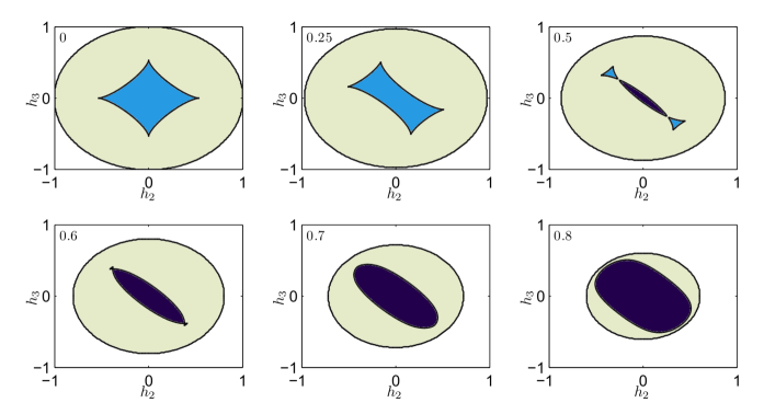
Figure 3: (Colour online) Cross-sections of the bifurcation surface at constant positive values of the bifurcation parameter $\mu$ (shown in top left of panels). The black regions correspond to the OS, while the light and grey regions (green and and blue online) correspond to 1 or 2 stable TWs, respectively. The outer circles represent the cuts through the sphere $\mu^{2}+h_{2}^{2}+h_{3}^{2}=1$ (where $k_{2}=0$). The bifurcation surface cuts look identical for negative $\mu$, but are rotated by $\pi/2$.

The bifurcation surface in Figure 2 separates the parameter space into four distinct regions. There is a bounded “Walker regime” around the origin, where the $k_{2}$-anisotropy dominates the dynamics (the origin is where $k_{2}=1$) and there are two stable Walker-like TW solutions. There are two bowl-shaped surfaces which separate the Walker regime from the north and south poles of the unit ball (at $\mu=\pm 1$). The OS is valid in the interior of the bowls. In the fourth region, which lies outside the bowls and the Walker regime, the transverse field dominates the dynamics (the boundary of the ball is where $k_{2}=0$), and there is a single stable TW solution. Sections of the bifurcation surface at several constant values of $\mu$ are shown in Figure 3).

Finally, we note that the roots $\mu$ of the quartic equation (57) can be expressed explicitly in terms of values of the parameters $k_{2}$, $h_{2}$ and $h_{3}$. However, these closed form analytic expressions for the bifurcation points are rather lengthy and, for this reason, are not reported in this paper.

4 Examples

4.1 Field-driven Motion $(j=0)$

In the following section we set the applied current $j=0$, and examine the asymptotic behaviour of solutions in more detail, for several regimes of the parameters $h_{1},h_{2},h_{3}$ and $k_{2}$. This provides the leading-order behaviour of both travelling waves and oscillating solutions, and the bifurcation points between them.

4.1.1 Walker Case: $h_{2}=h_{3}=0$

In the case of no transverse applied field $(h_{2}=h_{3}=0)$, an exact solution to the full nonlinear equation is known: the Walker solution. Here we show that our asymptotic method provides the essential features of the Walker solution, correctly predicts the so-called breakdown field, and also describes the motion beyond the breakdown field.

The ODE (38) for $\varphi_{0}$ reduces to

$$\dot{\varphi}_{0}={\frac{\alpha k_{2}}{2}\sin 2\varphi_{0}-h_{1}}.$$ (58)

In this case, there are just two possible solution types: $F(\varphi_{0})$ can now have either four zeros or no zeros (or two zeros at a bifurcation point). The critical driving field $h_{1,c}$ for the transition from the case of four zeros to that of none is easy to find; it occurs when

$$|h_{1}|=h_{1,c}:=\frac{\alpha k_{2}}{2}.$$ (59)

This is the same as the breakdown field in the exact Walker solution, and is now the only bifurcation in the equation.

Firstly, consider the case $\left|h_{1}\right|<h_{1,c}$. In this regime (58) has four fixed points, and two of them are stable, corresponding to TW solutions. The orientation angle of the DW can be found as a function of $h_{1}$ and $k_{2}$ by solving

$$\sin 2\varphi_{0}=\frac{h_{1}}{h_{1,c}}=\frac{2h_{1}}{\alpha k_{2}},$$ (60)

which again is the same as the value of $\varphi_{0}$ found in the exact Walker solution. As expected for a TW solution, $\varphi_{0}$ is found independent of $\tau$. The velocity of the travelling wave is given by the formula (43) and reads

$$\dot{x}_{*}=-h_{1}\left(\alpha+\frac{1}{\alpha}\right).$$ (61)

This is the leading-order term of the DW velocity predicted by the full nonlinear Walker solution. Combining the above expression for $\varphi_{0}$ with the DW profile $\theta_{0}(\xi)$, given by equation (15), we obtain the full leading-order behaviour of the travelling wave solution corresponding to the Walker solution. In addition, our asymptotic analysis correctly reproduces an exact expression for the breakdown field $h_{1,c}$.

Now consider the regime where $h_{1}>h_{1,c}$, in which the ODE (58) has no fixed points. The equation can be simply solved by separation of variables to find an OS

$$\tan\varphi_{0}=\frac{h_{1,c}}{h_{1}}-\frac{\sqrt{h_{1}^{2}-h_{1,c}^{2}}}{h_{1}}\tan\left(\tau\sqrt{h_{1}^{2}-h_{1,c}^{2}}\right).$$ (62)

In particular, we find that $\varphi_{0}$ is a periodic (modulo $2\pi$) function of $\tau$, with period $T={2\pi/}{\sqrt{h_{1}^{2}-h_{1,c}^{2}}}$. Physically, the magnetization DW precesses with an angular velocity $\dot{\varphi}_{0}$, which itself oscillates in time (but remains close to a constant value, see Figure 4). The average precessional velocity can be calculated by integrating $\dot{\varphi}_{0}$ over one period of the superimposed oscillations:

$$\left<\dot{\varphi}_{0}\right>=\frac{\sqrt{h_{1}^{2}-h_{1,c}^{2}}}{2\pi}\int_{a}^{a+T}\dot{\varphi}_{0}\,\,\mathrm{d}\tau.$$ (63)

Now, since

$$\bigg{[}{\varphi_{0}(\tau)}\bigg{]}_{\tau=a}^{\tau=a+T}=-\operatorname{sgn}(h_{1})2\pi,$$

we find

$$\left<\dot{\varphi}_{0}\right>=-\operatorname{sgn}(h_{1})\sqrt{h_{1}^{2}-h_{1,c}^{2}},$$ (64)

where $\operatorname{sgn}(\cdot)$ is the signum function. The precessional velocity changes monotonically with $h_{1}$, and approaches zero as $h_{1}\rightarrow\pm h_{1,c}$. When $|h_{1}|\gg h_{1,c}$, the precessional velocity approaches $-h_{1}$. This is equivalent to setting $k_{2}=0$ in (58).

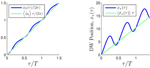
Figure 4: (Colour online) Walker case: temporal profiles of $\varphi_{0}(\tau)$ (left) and $x_{*}(\tau)$ (right). The dark curves (blue online) represent the explicit solutions, while the light lines (green online) show the average precession and propagation.

The average translational velocity can then be found from the formula (53):

$$\left<\dot{x}_{*}\right>=-h_{1}\left(\alpha+\frac{1}{\alpha}\right)+\frac{1}{\alpha}\operatorname{sgn}(h_{1})\sqrt{h_{1}^{2}-h_{1,c}^{2}}.$$ (65)

This coincides with the travelling wave velocity for $|h_{1}|=h_{1,c}$, and decreases in magnitude as $|h_{1}|$ increases beyond $h_{1,c}$. For $|h_{1}|\gg h_{1,c}$, the OS velocity approaches $-\alpha h_{1}$, which is consistent with the known exact solution of the LLG equations in the case of $k_{2}=0$ (the precessing solution – see Goussev et al. 2010). Finally, we note that since we have an analytic expression for $\varphi_{0}(\tau)$ in the oscillating regime, we can also find the velocity $\dot{x}_{*}(\tau)$ and hence the position $x_{*}(\tau)$ explicitly, though the expressions are quite unwieldy. See Figure 4 for a plot of the DW position as a function of $\tau$.

4.1.2 Maximal travelling wave velocity

We investigate the maximal travelling wave velocity in the case of $j=0$. From (43), the TW velocity is given by

$$\dot{x}_{*}=-h_{1}(\alpha+\alpha^{-1}),$$ (66)

which is valid for $h_{1}\leq h_{1,c}$. The maximum velocity is obtained for $|h_{1}|=h_{1,c}$. The critical field $h_{1,c}$ is the largest root of the quartic equation (57); equivalently (c.f. Eqs. (38) and (29)), we have that

$$|h_{1,c}|=\max_{\varphi_{0}}|h_{1}|=\max_{\varphi_{0}}\left|\alpha\Gamma\right|.$$ (67)

Figure 6 shows the dependence of the DW propagation velocity on $h_{1}$ for some representative nonzero values of $k_{2},h_{2}$ and $h_{3}$, and, illustrates the sharp velocity maximum attained at $h_{1}=h_{1,c}$.

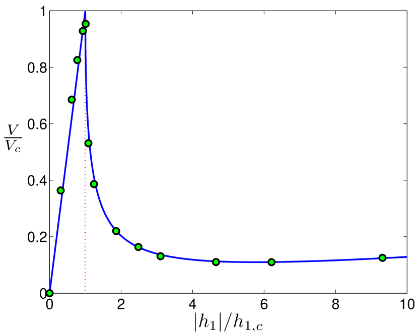
Figure 5: Normalized average velocity of DW as a function of normalized driving field. Parameter values: $k_{2}=0.2,h_{2}=h_{3}=0.1.$ The curve is the analytical prediction; the points are computed from numerically from the LLG equation (1).

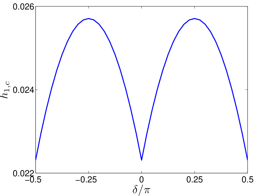
Figure 6: Variation of critical driving field, $h_{1,c}$, with angle of transverse field, $\delta$. Fixed parameters: $(k_{2}=0.2,\alpha=0.1,h_{T}=0.1)$.

Next, letting $h_{T}=\sqrt{h_{2}^{2}+h_{3}^{2}}$ denote the strength of the transverse field and $\delta=\arctan(h_{3}/h_{2})$ the angle between the transverse field and the hard-anisotropy axis, we seek to maximize $h_{1,c}$ with respect to $\delta$. From Eq. (67), this is obtained by maximising $|\Gamma|$ over both $\varphi_{0}$ and $\delta$. Critical points of $\Gamma$ with respect to $\varphi_{0}$ and $\delta$ are given by

$${\partial\Gamma\over\partial\varphi_{0}} ={\pi h_{T}\over 2}\cos(\varphi_{0}-\delta)-k_{2}\cos 2\varphi_{0}=0,$$ (68)

$${\partial\Gamma\over\partial\delta} =-{\pi h_{T}\over 2}\cos(\varphi_{0}-\delta)=0.$$ (69)

From these equations, it is straightforward to obtain

$$\cos 2\varphi_{0}^{c}=0,$$ (70)

and hence $\varphi_{0}^{c}\in\left\{{\pi\over 4},{3\pi\over 4},{5\pi\over 4},{7\pi\over 4}\right\}$. Thus, we establish that $|\Gamma|$ (and hence $|h_{1,c}|$) is maximized when $\delta\in\left\{{\pi\over 4},{3\pi\over 4},{5\pi\over 4},{7\pi\over 4}\right\}$. This corresponds to $h_{2}=\pm h_{3}$. A numerical confirmation of this result is presented in Figure 6.

It is straightforward to show (we omit the argument) that the critical field is a strictly increasing function of $k_{2}$ and $h_{T}$. Choosing $\delta$ to maximise $h_{1,c}$, we obtain

$$h_{1,c}=\frac{\alpha k_{2}}{2}+\frac{\alpha\pi h_{T}}{2}.$$ (71)

This analysis suggests that the most efficient way to get the fastest domain wall propagation, using constant applied fields, is to use a material with strong transverse anisotropy (large $k_{2}$) and apply a transverse magnetic field at an angle $\pi/4$ with the anisotropy axis.

4.2 Current-driven Motion $(\mathbf{h}_{a}=0)$

We consider the case of DW motion driven by a current applied along the wire. That is, we set $\mathbf{h}_{a}=0$, and examine the DW dynamics under the influence of $j$ and $k_{2}$ only. This problem has been widely studied in the literature (Thiaville et al. 2005; Mougin et al. 2007; Yan et al. 2010). It is straightforward to show that exact solutions of the LLG equation (1) can be found in two distinct regimes of $j$ and $k_{2}$. When $k_{2}=0$, there is a solution for arbitrary $j$ analogous to the precessing solution of field-driven motion (Goussev et al. 2010) given by

$$\theta(x,t)=\theta_{0}(x-x_{*}(t)),\quad\dot{x}_{*}(t)=\frac{-j(1+\alpha\beta)}{1+\alpha^{2}},\quad\dot{\varphi}(t)=\frac{\alpha-\beta}{1+\alpha^{2}}j,$$ (72)

where $\theta_{0}$ is the profile given in equation (15). When $k_{2}>0$ there is a TW solution for constant $j$ up to a certain critical value $j_{W}$, analogous to the Walker solution, given by

$$\theta=\theta_{0}\left(\frac{x-Vt}{\gamma}\right),\quad V=-\frac{\beta}{\alpha}j,\quad\sin 2\varphi=\frac{j}{j_{W}},\quad j_{W}={\alpha(1+\alpha^{2})k_{2}\gamma\over 2(\beta-\alpha)},$$ (73)

where $\gamma=(1+K_{2}\cos^{2}\varphi)^{-1/2}$ is the usual Walker scaling factor. This solution breaks down and produces an OS at values of $|j|$ above $|j_{W}|$. Using our perturbation analysis, we are able to characterize the leading-order behaviour of TWs and OSs, and the breakdown current. We then briefly discuss the propagation velocity of a DW in the current-driven case, where there are significant differences from the field-driven case depending on the relative sizes of the damping parameters $\alpha$ and $\beta$.

4.2.1 Leading-order behaviour

Setting $\mathbf{h}_{a}=0$ in equations (27) and (28) yields the equations for $\varphi_{0}(\tau)$ and $x_{*}(\tau)$:

$$\dot{\varphi}_{0}={\alpha k_{2}\over 2}\sin 2\varphi_{0}-\frac{(\beta-\alpha)}{1+\alpha^{2}}j,\quad\dot{x}_{*}=-{k_{2}\over 2}\sin 2\varphi_{0}-\frac{1+\alpha\beta}{1+\alpha^{2}}j.$$ (74)

The critical current is straightforward to calculate from (74), and is given by

$$j_{c}:={\alpha(1+\alpha^{2})k_{2}\over 2(\beta-\alpha)}.$$ (75)

This determines the only bifurcation point in the system. Note, unlike in the applied field (Walker) case, where the critical field matches the exact expression for the Walker breakdown field, the above expression for the critical current is not exact, but coincides with the leading-order term of the Taylor expansion in $k_{2}$ of the corresponding exact result. However, we shall see that an expression for the propagation velocity that we obtain is exact (unlike in the applied field case).

We have two regimes to consider: $|j|<|j_{c}|$ and $|j|>|j_{c}|$. From the same arguments as in the previous section, the case $|j|<|j_{c}|$ gives $\dot{\varphi}_{0}=0$, requiring us to solve

$${\alpha k_{2}\over 2}\sin 2\varphi_{0}-\left(1+\alpha^{2}\right)^{-1}(\beta-\alpha)j=0.$$ (76)

This yields two stable TW solutions (as in the Walker case of field-driven motion) which satisfy

$$\sin 2\varphi_{0}=\frac{j}{j_{c}},$$ (77)

and have the propagation velocity given by

$$\dot{x}_{*}=-{\beta\over\alpha}j.$$ (78)

This velocity is the same as that of the known exact TW solution.

For the regime $|j|>|j_{c}|$, we get an oscillating solution similar to (62), namely

$$\tan\varphi_{0}={j_{c}\over j}-{\sqrt{j^{2}-j_{c}^{2}}\over j}\tan\left({(\beta-\alpha)\over 1+\alpha^{2}}\tau\sqrt{j^{2}-j_{c}^{2}}\right).$$ (79)

The corresponding average precessional and translational velocities are given by

$$\left\langle\dot{\varphi_{0}}\right\rangle =-\operatorname{sgn}(j)\left(\frac{\beta-\alpha}{1+\alpha^{2}}\right)\sqrt{j^{2}-j_{c}^{2}},$$ (80)

$$\left\langle\dot{x}_{*}\right\rangle =-\frac{\beta}{\alpha}j+\operatorname{sgn}(j)\left(\frac{\beta-\alpha}{\alpha(1+\alpha^{2})}\right)\sqrt{j^{2}-j_{c}^{2}}.$$ (81)

It is interesting to note that in this current-driven case, the way the DW velocity varies with the applied current is subtly different from that in the applied field case. In particular, the current-velocity characteristic changes dramatically with the sign of $\beta-\alpha$ (see Figure 7).

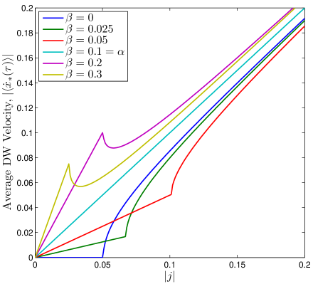
Figure 7: (Colour online) Average velocity of DW as a function of applied current, for different values of the nonadiabatic damping parameter $\beta$. Fixed parameter values: $k_{2}=0.1,\alpha=0.1.$

When $\beta>\alpha$ the curves have a similar shape to the velocity-$h_{1}$ characteristic in Figure 6; the velocity drops sharply as the current is increased above the critical current, then resumes a linear behaviour after that. However, here the average velocity of the OS exceeds the maximal velocity of the TW (for fixed $\beta$) at an applied current not much greater than the critical current:

$$|j|>|j_{c}|\left(\frac{\beta^{2}(1+\alpha^{2})^{2}+(\beta-\alpha)^{2}}{\beta^{2}(1+\alpha^{2})^{2}-(\beta-\alpha)^{2}}\right)\sim|j_{c}|.$$ (82)

This is to be compared with the field-driven case, where the average velocity of the OS in the Walker regime only exceeds the maximum velocity of the TW solution when $h_{1}\gg h_{1,c}$:

$$|h_{1}|>h_{1,c}\left(1+\frac{2}{\alpha^{4}+2\alpha^{2}}\right)\sim\frac{h_{1,c}}{\alpha^{4}}.$$ (83)

When $\beta=\alpha$ the critical current is infinite (this is clear from (75)), and so the TW behaviour persists for all applied currents. When $\beta<\alpha$ the velocity rises sharply above the critical current, and the average velocity of the OS always exceeds the maximal TW velocity. This behaviour is in accordance with that found in previous literature (Thiaville et al. 2005), and is particularly evident from the fact that when $\beta=0$ the TW velocity vanishes, and the DW does not undergo any motion until $j$ exceeds $j_{c}$, and the OS appears.

4.2.2 Multiple Domain Walls

We examine the dynamics of a finite string of $N$ current-driven DWs. A typical multiple DW profile is given by

$$\theta_{N}(\xi,\tau)=\displaystyle\sum_{n=1}^{N}\theta\left((-1)^{n+1}\xi_{n},\tau\right),$$ (84)

where $\xi_{n}=x-x_{*,n}(\tau)$ and each $x_{*,n}$ is such that adjacent DWs do not overlap at $\tau=0$. It is clear that when multiple DWs are present, a tail-to-tail profile must have head-to-head profiles on either side of it, and vice versa. Figure 8 shows schematically a tail-to-tail DW on the left followed by a head-to-head DW on the right, with their respective leading-order dynamics (as calculated in the following analysis).

Figure 8: Adjacent DW profiles with leading-order translational and precessional velocities.

In Section II we analysed the dynamics of the tail-to-tail profile $(\theta,\varphi)$ and found the leading-order precessional and translational velocities (27) and (28). The dynamics of the head-to-head profile $(\tilde{\theta},\tilde{\varphi})$ may be similarly analysed, and one finds that

$$\dot{\tilde{\varphi}}_{0}=-\dot{\varphi}_{0},\quad\dot{\tilde{x}}_{*}=\dot{x}_{*},$$ (85)

and thus $\dot{x}_{*,n}=\dot{x}_{*}$. Unlike the case of field-driven strings of DWs (Goussev et al. 2010), in which adjacent head-to-head and tail-to-tail DWs move in opposite directions but precess in the same direction, all current-driven DWs travel in the same direction, but with adjacent DWs precessing in opposite directions.

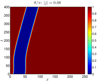
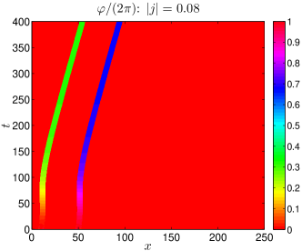
Figure 9: (Colour online) Spatiotemporal Magnetization Profile—TW behaviour: two adjacent DWs driven by applied current $j=-0.08$. Fixed parameter values are $\alpha=0.1$, $\beta=0.2$, $k_{2}=0.2$.

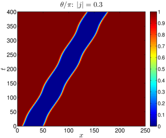
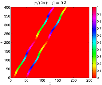
Figure 10: (Colour online) Spatiotemporal Magnetization Profile—OS behaviour: two adjacent DWs driven by applied current $j=-0.3$. $\alpha=0.1$, $\beta=0.2$, $k_{2}=0.2$.

Figures 9 and 10 show the spatiotemporal magnetization profiles of a TW and an OS, obtained from numerical solution of the LLG equation (1). In each plot, the initial condition is given by two adjacent optimal DW profiles with orientation $\varphi=0$. In the TW case we see that the translational velocities of the two DWs, after some initial transient, become constant and equal to each other. The DWs rotate in the opposite directions (at the same rate) and eventually, as expected, reach a steady state, in which the orientation of one DW is opposite to that of the other. In the OS case, we again find the DWs moving in the same direction, while rotating in the opposite directions (again at the same rate). The velocity of this OS is, in fact, greater than that of the TW shown. The ability to drive DWs in the same direction has a direct application in the recently proposed race-track memory architecture (Parkin et al. 2008; Hayashi et al. 2008)

5 Conclusion

We have presented a new asymptotic analysis of domain wall dynamics in one-dimensional nanowires, governed by the Landau–Lifshitz–Gilbert equation. The approach is valid when the hard-axis anisotropy, applied magnetic fields and currents are small compared to the exchange coefficient and easy-axis anisotropy.

Our approach covers both travelling-wave type and oscillatory domain wall motion. We present asymptotic formulas for the domain wall velocity and orientation angle in the travelling wave case, and for the average drift velocity and precession speed in the oscillatory case. Additionally, we are able to calculate the critical values of driving field (or current) for the transitions from travelling wave to oscillatory behaviour, as bifurcations in the associated dynamical system. This transition is analogous to the Walker breakdown, and is a generic feature of domain wall motion. The formulas given are valid for any combinations of the parameters (hard-axis anisotropy, applied fields and currents), provided the small parameter condition is met. We also present the leading-order domain wall magnetization profile and the next-order correction.

We discuss several special cases and demonstrate that our approach accurately reproduces the essential features of domain wall motion. We compare results of our asymptotic analysis with both numerical and exact analytical results (when available) and find them to be in good agreement.

We would like to acknowledge support from the EPSRC (grant EP/I028714/1 to VS, and doctoral training awards to CS and RGL).