Adoption of bundled services with network externalities and correlated affinities

Abstract

The goal of this paper is to develop a principled understanding of when it is beneficial to bundle technologies or services whose value is heavily dependent on the size of their user base, i.e., exhibits positive exernalities. Of interest is how the joint distribution, and in particular the correlation, of the values users assign to components of a bundle affect its odds of success. The results offer insight and guidelines for deciding when bundling new Internet technologies or services can help improve their overall adoption. In particular, successful outcomes appear to require a minimum level of value correlation.

Roch Guérin, Jaudelice C. de Oliveira, and Steven Weber, 2013. Adoption of bundled services with network externalities and correlated affinities.

1 Introduction

Many Internet technologies, applications, and services have value that increases with the size of their user base, i.e., they exhibit positive externalities or network effects. Externalities are well-known [Cabral (1990)] to have dual effects on the adoption pattern of services. Adoption rapidly accelerates after passing a critical threshold (until the market starts saturating), but reaching this critical level of adoption is often slow and difficult. In practice, services that fail often do so during this early stage, as many potential adopters see a cost that exceeds the (low) initial value of the service. This is commonly mentioned as an explanation for the limited or stalled adoption of many Internet security protocols [Ozment and Schechter (2006)].

A common approach (see again [Ozment and Schechter (2006)]) to overcome this initial hurdle is to bundle services, in the hope that the bundle has broader appeal and is, therefore, able to overcome early adoption inertia. The main unknown is the extent to which dependencies (as measured by a joint distribution) or correlation in how users value the individual services influence their adoption decision for the bundle. We illustrate this next by way of examples, which also (and more importantly) demonstrate the diversity of Internet services for which this arises.

1.1 Anonymous communications and secure distributed storage

Anonymous communication systems have been available for some time, e.g., see [Fernández Franco (2012)] for a recent survey, but in spite of a recent rise in both profile [Arthur (2013)] and usage [Brewster (2013)], they remain relatively marginal, i.e., have not yet attracted a large user-base. This can affect their robustness and their ability to deliver strong anonymity guarantees (mixing traffic from more users and tapping into the resources contributed by those users can improve both anonymity and robustness, at least in P2P based implementations of such systems).

Overcoming the limited appeal (to users) of anonymous communications and increasing the number of users such a system can tap into, can be realized by bundling it with another service. Ideally, this other service should exhibit technical synergies with anonymous communications so as to facilitate a joint implementation. Secure distributed storage is a possible candidate. It enables the automatic and encrypted backup of local files over a distributed set of network peers (see BuddyBackup for an example), and shares with anonymous communications a reliance on cryptographic primitives and protocols, as well as a value that grows with its number of adopters (more users likely means a more reliable system). The main question is whether combining those two services can increase adoption for both. The answer depends on the cost versus value of the bundle, and how this varies across users.

The cost of the bundle consists of the communication (bandwidth), processing, and storage costs of the two services, with anonymous communications calling mostly for bandwidth and processing resources, and secure distributed storage requiring primarily storage resources and to a lesser extent processing and communication resources. Because the two services have mostly independent needs, those costs should be approximately additive. The value a user assigns to the bundle depends on her level of usage of anonymous communications and reliance on secure distributed storage as a means of preserving and accessing her personal data. This value will change as more users adopt the bundle (it improves the quality and reliability of both services), but the decisions of early adopters depend primarily on how they intrinsically value access to anonymous communication and secure distributed storage.

For illustration purposes, assume that within a given user population the stand-alone values of both services are uniformly distributed. However, to reflect the fact that secure distributed storage should be attractive to most users while anonymous communications will likely have more limited appeal, we assume that the stand-alone values of the former are in $[a,1],0<a<1,$ while they span the full $[0,1]$ range for the latter. In other words, most users view secure distributed storage as useful (valued at $\geq a$), while fewer assign a similar value (in the range $[a,1]$) to anonymous communications. Under those assumptions, correlation in user valuations clearly affects the number of early adopters the service bundle will attract. For example, it is relatively easy to show (see Section 4 for related derivation details) that the cost threshold beyond which there are no early adopters for the bundle is $2$ under perfect positive correlation, but only $a+1$ under perfect negative correlation.

1.2 Online discussion forums

Consider next the case of an online discussion forum dedicated to a particular topic. Participating in such a forum has some intrinsic value, e.g., from access to promotions and discounts on related products, but its core value often comes from the answers and advice it provides in response to users’ questions. To succeed, a forum must, therefore, accumulate a large enough “knowledge-base” and consequently achieve a critical mass of users. This can be challenging, as the added value from Q&A’s is essentially absent in the early stages, and promotions and discounts alone may be insufficient to attract enough early adopters. Combining the topics of multiple forums under a common umbrella is one way to address this challenge. The stand-alone value of such a “bundled” forum, e.g., promotions and discounts that now extend across more products, may appeal to a broader user base, and allow it to succeed where individual forums would not have. The question we seek to answer is again when and why this may be the case?

As with anonymous communications and secure distributed storage, whether a bundled forum attracts more early adopters, and therefore improves its odds of success, depends on its initial cost-benefit ratio relative to that of individual forums. The “cost” of joining a bundled forum, e.g., the amount of time needed to extract useful information, can be higher than that of more focused, single-topic forums. Its combined stand-alone value arguably depends on many factors, but a reasonable first approximation is again to assume that it is the sum of the stand-alone values (product promotions and discounts) associated with both topics. As in the previous example, whether this sum exceeds the cost of joining the forum, which determines the number of early adopters, depends to a large extent on the joint distribution of user valuations for the individual forums; an important measure of which is their correlation.

For purpose of illustration, consider a scenario where we contemplate merging two discussion forums, whose stand-alone values follow identical uniform distributions when measured across a population of users (they are of equal value on average). Assume further that for a given user, the values she sees in the two forums are either perfectly positively or perfectly negatively correlated, i.e., equal or diametrically opposed. Under perfect positive correlation, the stand-alone value that any user derives from the bundled forum is then simply twice the value she sees in either individual forum. If we assume that the cost of joining the bundled forum is also twice that of joining a single-topic forum, e.g., it takes twice as long to find relevant information, then it is easy to show that bundling has no impact on early adoption, and the bundled forum sees the same number of potential early adopters as either original forum. In contrast, when values are perfectly negatively correlated, all users now see the same (average) value from joining the bundled forum. In this case either no user or all users will be early adopters, depending on whether this average value is above or below the bundle’s cost. Hence, unlike the case of perfect positive correlation, bundling can significantly affect the number of early adopters.

1.3 Summary

As the above examples hopefully illustrated, correlation in how users value different services and/or technologies (and more generally their joint distribution) can have a significant effect on whether combining them in a bundle is beneficial. In the rest of this paper, we explore this issue in a systematic fashion. Section 2 offers a brief review of related works. Section 3 introduces our model for service adoption. Section 4 considers the case where user affinities for the services are represented as continuous uniform random variables. It first explores the extreme cases of perfect positive and negative correlation in Section 4.3 and Section 4.4, respectively, while Section 4.5 investigates the intermediate case of independent affinities. The latter section illustrates the difficulty of characterizing the bundle’s adoption under general correlation, and motivates the model of Section 5 where user affinities for the services are captured through correlated discrete (Bernoulli) random variables with parameterized correlation. Section 6 articulates the findings that emerge from the analysis, and numerically explores their robustness through limited extensions to the model. Section 7 offers a brief conclusion.

2 Related work

The topic of this paper is at the intersection of two major lines of work; product and technology diffusion, and product and service bundling.

Modeling how products and services diffuse through a population of potential users, i.e., are being adopted, is a topic of longstanding interest in marketing research with [Peres et al. (2010)] offering a recent review of available models and techniques. The models most relevant to our investigation are those based on the approach introduced in [Cabral (1990)] and extended in many subsequent works, which explore product diffusion in the presence of externalities using an adoption decision process that reflects the utility of individual users. As described in Section 3, the adoption model we rely on belongs to this line of work. However, and except for a few recent works that we review below, the aspect of bundling had not been incorporated in those investigations, and this is one of the aspects we focus on in the paper.

There has obviously been a significant literature devoted to bundling as a stand-alone topic (see [Venkatesh and Mahajan (2009)] for a recent review). The main goal of most of those works has typically been the development of optimal bundling and pricing strategies, and pricing is a dimension that is largely absent from our investigation in that service costs are assumed given and exogenous. Instead, our focus is mostly on how the joint distribution in service valuation across users (as measured through their correlation coefficient), determines whether the adoption level of a service bundle can exceed those of separate service offerings. Correlation in how users value different services and the impact this has on bundling strategies is in itself a topic that several prior works have explicitly taken into account, e.g., [Schmalensee (1984), McAfee et al. (1989), Bakos and Brynjolfsson (1999)]. In general, negative correlation in demand improves bundling’s benefits over separate offerings, although high marginal costs (compared to the average value of the bundle) can negate this effect. Conversely, a high positive correlation tends to yield the opposite outcome, i.e., favor separate (pure component) offerings. As highlighted in the examples of Section 1, our focus on maximizing adoption results in more nuanced outcomes, with correlation playing a more ambivalent role in determining the success of a bundled offering. Furthermore, early works on bundling did not account for the potential impact of externalities.

There are to-date only three works we are aware of [Prasad et al. (2010), Pang and Etzion (2012), Chao and Derdenger (2013)] that have investigated the problem of bundling products or services with externalities, and we briefly review how these papers differ from our investigation. First and as has been the norm in the bundling literature, those three papers all focus on optimal pricing strategies, while we assume that costs (prices) are exogenous parameters and instead seek to understand their impact (and that of other factors) on the adoption level of a bundled offering. Second, the impact of value (demand) correlation is essentially absent from those three prior works.

Specifically, [Prasad et al. (2010)] focuses on optimal pricing while assuming independent valuations for the two services. [Pang and Etzion (2012)] explores the joint offering of a product and a complementary service, where the latter exhibits positive externalities. As in [Prasad et al. (2010)], users’ valuations for the product and its complementary service are assumed independent, and there is no investigation of the potential impact of their correlation. [Chao and Derdenger (2013)] is cast in the context of a two-sided market (the two market sides create externalities), where the platform provider seeks to decide how to bundle and price new content with the platform it offers, given the existence of an installed based of users and content developers. The focus is again on optimal pricing strategies and bundling decisions, and there is no correlation between the value of the new content and that of earlier content. These are again important differences with our work, which furthermore does not involve the presence of an existing user base. As [Chao and Derdenger (2013)]’s title indicates and as the paper emphasizes (Section 2.2), this plays an important role in the platform’s strategic decisions. In contrast, our interest lies primarily in understanding how bundling can help nascent Internet services ultimately reach the high levels of adoption they need to realize their full value potential and succeed.

3 Mathematical model

In this section, we review the basic structure of the models on which we rely to capture the evolution of service adoption.

3.1 Separate (unbundled) service offerings

We consider a model for the adoption of multiple (two) services by a heterogeneous population of potential users. The perceived utility $V_{i}(x_{i}(t))$ of service $i\in\{1,2\}$ by a (random) user given that a fraction $x_{i}(t)\in[0,1]$ of the population has adopted the service at time $t$ incorporates three components: $i)$ the user’s affinity (stand-alone value) for the service (capturing users’ heterogeneity), $ii)$ the network externality tied to the adoption level of the service, and $iii)$ the service cost. Specifically:

$$V_{i}(x_{i}(t))=U_{i}+e_{i}x_{i}(t)-c_{i},~{}i\in\{1,2\},$$ (1)

where $i)$ $U_{i}\geq 0$ is the user’s (random) affinity for service $i$; $ii)$ $e_{i}\geq 0$ is the strength of the externality contribution for service $i$; and $iii)$ $c_{i}\geq 0$ is the cost of adopting service $i$. As is common, for analytical tractability we adopt a linear externality model.

When services are offered separately, users make adoption decisions for each based on their respective utilities:

$$\mbox{user adopts service $i$ at time $t$ with adoption level $x_{i}(t)$}~{}\Leftrightarrow~{}V_{i}(x_{i}(t))>0.$$

In particular, there is no “budget constraint” where adoption of one service by a user affects adoption of the other service by that user; this is natural given our focus on adoption costs, e.g., communication, storage, processing, etc., rather than pricing. However, while service adoption decisions are uncoupled, the random variables $(U_{1},U_{2})$, capturing heterogeneity in user affinity, may be correlated.

Denote as $h_{i}(x_{i})=\mathbb{P}(V_{i}(x_{i})>0)$ the probability a random user adopts service $i$ given an adoption level $x_{i}$. An equilibrium for this model is any $x_{i}^{*}$ such that

$$h_{i}(x_{i}^{*})=\mathbb{P}(U_{i}>c_{i}-e_{i}x_{i}^{*})=x_{i}^{*}.$$ (2)

When the two services are offered separately they achieve adoption equilibria $(x_{1}^{*},x_{2}^{*})\in[0,1]\times[0,1]$. One of our goals is to compare these equilibria to those realized when the two services are bundled, and characterize differences as a function of the model’s parameters $(e_{1},e_{2},c_{1},c_{2})$ and the joint distribution of $(U_{1},U_{2})$.

3.2 Bundled service offerings

Under bundling, a user must decide whether to adopt either both services or neither, i.e., we do not consider the case of mixed bundling where services are simultaneously offered as a bundle and separately. The basis for a user’s decision is now the aggregate utility she derives from the bundle:

$$\mbox{user adopts the bundle at time $t$}~{}\Leftrightarrow~{}V(x(t))>0,$$

where consistent with Eq. (1)

$$V(x(t))=V_{1}(x(t))+V_{2}(x(t))=U+ex(t)-c.$$ (3)

Here, $x(t)$ is the (common) adoption level of the bundled services. Note the assumption of additive values for the two services, i.e., $V(x(t))=V_{1}(x(t))+V_{2}(x(t))$, which implies that they are neither substitute nor complement. Under this assumption, $U=U_{1}+U_{2}$ is the aggregate intrinsic value of the bundled services, $e=e_{1}+e_{2}$ is the aggregate force of the externality, and $c$ is the aggregate cost, which for simplicity also satisfies $c=c_{1}+c_{2}$. Extending the model to account for instances where the two services are partial complements or substitutes, as well as for possible economies of scope in the cost of a service bundle is clearly of interest. Such extensions can be readily incorporated in the models, but add complexity. Furthermore, while they quantitatively affect adoption outcomes, i.e., if and when bundling is beneficial, the qualitative findings of the paper still hold, and in particular the importance of the joint distribution (correlation) of service affinities in the efficacy of bundling.

As with separate offerings, equilibria satisfy

$$h(x^{*})=\mathbb{P}(U>c-ex^{*})=x^{*}.$$ (4)

Our question can now be restated more formally: how do adoption equilibria $(x^{*},x^{*})$ under bundling compare with adoption equilibria $(x_{1}^{*},x_{2}^{*})$ when services are offered separately?

It remains to specify the joint distribution of service affinities (values a user assigns to each service) $(U_{1},U_{2})$. In Section 4 we consider the case where $(U_{1},U_{2})$ are uniform continuous random variables, while in Section 5 we assume that $(U_{1},U_{2})$ are uniform discrete (Bernoulli) random variables. Table 3.2 lists commonly used notation.

Notation $x_{i}(t)$ adoption level of (unbundled) service $i$ at time $t$ $x(t)$ adoption level of service bundle at time $t$ $x_{i}^{*},x^{*}$ equilibria adoption level for service $i$ and bundle $(U_{1},U_{2})$ random (unbundled) service affinities $U=U_{1}+U_{2}$ affinity for service bundle $(e_{1},e_{2})$ externality for (unbundled) services $1,2$ $e=e_{1}+e_{2}$ externality for service bundle $(c_{1},c_{2})$ costs for adopting (unbundled) services $1,2$ $c=c_{1}+c_{2}$ costs for adopting service bundle $(V_{1},V_{2})$ utility function for (unbundled) services $1,2$ $V=V_{1}+V_{2}$ utility function for service bundle $h_{i}(x_{i})=\mathbb{P}(V_{i}(x_{i})>0)$ probability of adoption of (unbundled) services $1,2$ $h(x)=\mathbb{P}(V(x)>0)$ probability of adoption of service bundle $l_{i}=\frac{c_{i}-1}{e_{i}}$ left adoption threshold for (unbundled) services $1,2$ $r_{i}=\frac{c_{i}}{e_{i}}$ right adoption threshold for (unbundled) services $1,2$ $l=\frac{c-2}{e}$ left adoption threshold for service bundle $m=\frac{c-1}{e}$ middle adoption threshold for service bundle $r=\frac{c}{e}$ right adoption threshold for service bundle $\rho$ correlation parameter for $(U_{1},U_{2})$ in (17) $p$ distribution parameter for $(U_{1},U_{2})$ in (5) $n$ population size for Monte-Carlo simulations

4 Continuous affinities

In this section, we assume $(U_{1},U_{2})$ are continuous uniform random variables on $[0,1]$. This assumption is sufficient to characterize the equilibria under separate service offerings, which we do in Section 4.1. The equilibria under bundled service offerings, however, depend upon the correlation between $(U_{1},U_{2})$, since the bundled affinity depends upon $U=U_{1}+U_{2}$. A distribution on $(U_{1},U_{2})$ with a parameterized correlation is presented in Section 4.2, but is difficult to work with in its general form. Consequently, we investigate the three special cases where $(U_{1},U_{2})$ are perfectly positively (Section 4.3) and negatively (Section 4.4) correlated, and independent (Section 4.5). The intent is to illustrate that different types of outcomes arise at the two correlation extremes, and confirm the difficulties associated with capturing the impact of intermediate correlation values when using continuous distributions. This then motivates the more tractable discrete model of Section 5, wherein we are able to more explicitly explore the impact of varying correlation. Numerical investigations are then used in Section 6.2 to verify that findings obtained with the simpler discrete model also hold under the continuous model.

4.1 Separate offerings

The following proposition characterizes the possible equilibria for separate service offerings when the user service affinities are uniform random variables.

Proposition 4.1.

When $U_{i}$ ($i\in\{1,2\}$) is uniformly distributed on $[0,1]$, the probability of user adoption of service $i$ in Eq. (2) becomes

$$h_{i}(x_{i})=\left\{\begin{array}[]{lrcccl}0,&&&x_{i}&\leq&l_{i}\\ e_{i}x_{i}+1-c_{i},&l_{i}&<&x_{i}&\leq&r_{i}\\ 1,&r_{i}&>&x_{i}&&\end{array}\right.$$ (5)

for adoption thresholds $l_{i}\equiv\frac{c_{i}-1}{e_{i}}$ and $r_{i}\equiv\frac{c_{i}}{e_{i}}$. The three possible equilibria are $x_{i}^{*}\in\{0,(1-c_{i})/(1-e_{i}),1\}$. The conditions for each equilibrium (eq.) are:

$$0\mbox{ is stable eq.} \Leftrightarrow c_{i}>1$$

$$\frac{1-c_{i}}{1-e_{i}}\mbox{ is stable eq.} \Leftrightarrow e_{i}<c_{i}<1$$

$$\frac{1-c_{i}}{1-e_{i}}\mbox{ is unstable eq.} \Leftrightarrow 1<e_{i}<c_{i}$$

$$1\mbox{ is stable eq.} \Leftrightarrow e_{i}>c_{i}$$

The lowest stable equilibrium (lseq.) adoption level for each $(c_{i},e_{i})$ is

$$0\mbox{ is lseq.} \Leftrightarrow c_{i}>1$$

$$\frac{1-c_{i}}{1-e_{i}}\mbox{ is lseq.} \Leftrightarrow e_{i}<c_{i}<1$$

$$1\mbox{ is lseq.} \Leftrightarrow c_{i}<\min\{e_{i},1\}$$

The proof of Prop. 4.1 is straightforward and is omitted. Note that the equilibria conditions are a cover but not a partition of the $(c_{i},e_{i})$ plane, while the lseq. conditions are a partition of the $(c_{i},e_{i})$ plane (see Fig. 6 in the appendix for an illustration). Note also that the notion of lowest stable equilibrium $(lseq.)$ is natural is our setting, where we consider services that have an initial adoption level of $0$ when first offered, i.e., $x_{i}(0)=0$, so that the lseq. will be the achieved equilibrium. The conditions on the equilibria are also intuitive: zero adoption results when the costs are high, full adoption results when the externality effect outweighs the cost, and partial adoption results when costs are low but outweigh the externality effect.

4.2 Bundling under general correlation

The equilibria under bundled service offerings with continuous uniform affinities $(U_{1},U_{2})$ depend upon the correlation between them. There are many ways to generate random variables with parametrized correlation. We rely on a standard approach [Pearson (1907), Hotelling and Pabst (1936)] (see the Appendix, Section A.1 for details) to generate a pair of uniform random variables $(U_{1},U_{2})$ with correlation coefficient $\rho$ for any value $\rho\in[-1,1]$. The approach uses a pair of independent standard normal random variables as its starting point, so that the joint distribution $F_{U_{1},U_{2}}(u_{1},u_{2})$, the distribution of the aggregate service affinity $F_{U}(u)$ for $U=U_{1}+U_{2}$, and the resulting probability of adoption $h(x)$, can all be described in terms of the standard normal CDF $F_{Z}$.

As seen in the Appendix, the resulting expressions are, in general, rather unwieldy, and for illustration purposes, we restate below the expression for $h(x)$ that can be used to determine adoption equilibria.

$$h(x)=\left\{\begin{array}[]{lrcccl}0,&&&x&\leq&l\\ 2-(c-ex)-\displaystyle\int_{c-ex-1}^{1}F_{Z}\left(\frac{F_{Z}^{-1}(c-ex-v)-\rho F_{Z}^{-1}(v)}{\sqrt{1-\rho^{2}}}\right)\mathrm{d}v,&l&<&x&\leq&m\\ 1-\displaystyle\int_{0}^{c-ex}F_{Z}\left(\frac{F_{Z}^{-1}(c-ex-v)-\rho F_{Z}^{-1}(v)}{\sqrt{1-\rho^{2}}}\right)\mathrm{d}v,&m&<&x&\leq&r\\ 1,&r&<&x&&\end{array}\right.$$ (6)

for adoption thresholds $l\equiv\frac{c-2}{e}$, $m\equiv\frac{c-1}{e}$, and $r\equiv\frac{c}{e}$.

The equilibria under bundling are the solutions of $h(x)=x$. As evident from Eq. (6), this is a difficult equation to work with. This motivates focusing on the three specific cases of perfect positive ($U_{1}=U_{2}$) and negative ($U_{1}=1-U_{2}$) correlation, as well as independence, i.e., $\rho\in\{-1,0,+1\}$.

4.3 Perfect positive correlation

Specializing for $\rho=1$ Props. A.4 and A.8 of the Appendix yields the joint and sum distributions for uniform random variables $(U_{1},U_{2})$ satisfying $U_{1}=U_{2}$, and thus $U=U_{1}+U_{2}$ is uniform over $[0,2]$:

$$F_{U_{1},U_{2}}(u_{1},u_{2})=\min\{u_{1},u_{2}\} f_{U_{1},U_{2}}(u_{1},u_{2})=\mathbf{1}_{u_{1}=u_{2}}$$

$$F_{U}(u)=u/2,~{}u\in[0,2] f_{U}(u)=1/2,~{}u\in[0,2].$$

Because the aggregate affinity is uniformly distributed on $[0,2]$, the resulting equilibria are of the same form as in Prop. 4.1 after replacing $e_{i}$ and $c_{i}$ by $e/2$ and $c/2$, respectively. Thus we have the following corollary to Prop. A.12 and Prop. 4.1.

Corollary 4.2.

The probability of bundle adoption $h(x)$ in Prop. A.12 under aggregate affinity $U=U_{1}+U_{2}$ formed from perfectly positively correlated uniform affinities $(U_{1},U_{2})$ satisfying $U_{1}=U_{2}$ is

$$h(x)=\left\{\begin{array}[]{lrcccl}0,&&&x&\leq&l\\ \frac{e}{2}x+1-\frac{c}{2},&l&<&x&\leq&r\\ 1,&r&<&x&&\end{array}\right.$$ (7)

The three possible equilibria are $x^{*}\in\{0,(2-c)/(2-e),1\}$. The conditions for each equilibrium (eq.) are:

$$0\mbox{ is stable eq.}\Leftrightarrow c>2,\quad 1\mbox{ is stable eq.}\Leftrightarrow e>c$$

$$\frac{2-c}{2-e}\mbox{ is stable eq.}\Leftrightarrow e<c<2,\quad\frac{2-c}{2-e}\mbox{ is unstable eq.}\Leftrightarrow 2<e<c$$

The lowest stable equilibrium (lseq.) adoption level for each $(c,e)$ is

$$0\mbox{ is lseq.}\Leftrightarrow c>2,\quad\frac{2-c}{2-e}\mbox{ is lseq.}\Leftrightarrow e<c<2,\quad 1\mbox{ is lseq.}\Leftrightarrow c<\min\{e,2\}$$

The next part of the analysis is to compare the lowest stable equilibria under separate ($(x_{1}^{*},x_{2}^{*})$) and bundled ($(x^{*},x^{*})$) offerings as a function of the system parameters $(e_{1},e_{2},c_{1},c_{2})$. The results are shown below.

$$\begin{array}[]{c|cc||ccc}&&&0&\frac{2-c}{2-e}&1\\ \hline\cr&&&c>2&e<c<2&c<e\land 2\\ \hline\cr\hline\cr(0,0)&c_{1}>1&c_{2}>1&SS&WW&WW\\ &&&\mbox{True}&\mbox{False}&\mbox{False}\\ \hline\cr\left(0,\frac{1-c_{2}}{1-e_{2}}\right)&c_{1}>1&e_{2}<c_{2}<1&SL&WL\mbox{ or }WW&WW\\ \hline\cr(0,1)&c_{1}>1&c_{2}<e_{2}\land 1&SL&WL&WS\\ \hline\cr\left(\frac{1-c_{1}}{1-e_{1}},0\right)&e_{1}<c_{1}<1&c_{2}>1&LS&LW\mbox{ or }WW&WW\\ \hline\cr(1,0)&c_{1}<e_{1}\land 1&c_{2}>1&LS&LW&SW\\ \hline\cr\left(\frac{1-c_{1}}{1-e_{1}},\frac{1-c_{2}}{1-e_{2}}\right)&e_{1}<c_{1}<1&e_{2}<c_{2}<1&LL&WL\mbox{ or }LW&WW\\ &&&\mbox{False}&&\mbox{False}\\ \hline\cr\left(\frac{1-c_{1}}{1-e_{1}},1\right)&e_{1}<c_{1}<1&c_{2}<e_{2}\land 1&LL&WL&WS\\ &&&\mbox{False}&&\\ \hline\cr\left(1,\frac{1-c_{2}}{1-e_{2}}\right)&c_{1}<e_{1}\land 1&e_{2}<c_{2}<1&LL&LW&SW\\ &&&\mbox{False}&&\\ \hline\cr(1,1)&c_{1}<e_{1}\land 1&c_{2}<e_{2}\land 1&LL&LL&SS\\ &&&\mbox{False}&\mbox{False}&\mbox{True}\\ \hline\cr\end{array}$$

The nine rows are lowest stable equilibria $(x_{1}^{*},x_{2}^{*})$ under separate offerings, with $x_{i}^{*}\in\{0,(1-c_{i})/(1-e_{i}),1\}$ for $i\in\{1,2\}$. The third column corresponds to the lowest stable equilibria $(x^{*},x^{*})$ under bundling with $x^{*}\in\{0,(2-c)/(2-e),1\}$. Each combination of row and third column entry, say $(x_{1}^{*},x_{2}^{*},x^{*})$, is a possible equilibrium triple without and with bundling. The second column gives the conditions on $(c_{1},c_{2},e_{1},e_{2})$ for each $(x_{1}^{*},x_{2}^{*})$ to be the lowest stable equilibria under separate offerings, and the second row of the third column gives the conditions on $(c,e)$ for each $x^{*}$ to be the lowest stable equilibria under bundling.

Each third column entry is labeled with a pair of letters $(\Delta_{1},\Delta_{2})$ with $\Delta_{i}\in\{L,S,W\}$ for $i\in\{1,2\}$ representing (L)ose, (S)ame, and (W)in, and denoting the change in equilibrium under bundling for that service. For example, $SL$ means the equilibrium for service $1$ stayed the same ($x_{1}^{*}=x^{*}$), while the equilibrium for service $2$ decreased ($x_{2}^{*}>x^{*}$). The notation $a\land b$ in the inequalities in the second column, simply means that the inequality needs to be satisfied for both $a$ “AND” $b$. The word “True” indicates the equilibrium for the column always results for the equilibria in the corresponding row, e.g., when $c_{1}>1$ and $c_{2}>1$, the bundled equilibrium $0$ always result for the separate equilibria $(0,0)$ because the conditions on $c_{1}$ and $c_{2}$ imply $c>2$. Conversely, the word “False” indicates the equilibrium for the column is never feasible for the equilibria in the corresponding row.

There are nine possible tuples. Under perfectly positively correlated user valuations, the bundle’s valuation is essentially a weighted sum of the valuations of the individual services, so that most outcomes involve a trade-off between improving (or maintaining) the adoption of one service and worsening (or maintaining) that of the other. Of note is the fact that a $LL$ outcome is not feasible. This is because, a bundle equilibrium of $0$ only arises when the less valuable service also has an equilibrium of $0$ when offered alone, which results in a $SL$ (or $LS$) outcome. Because of the effect of externalities, the converse is, however not true, i.e., $WW$ outcomes can be realized.

$WW$ outcomes typically arise when one technology has a high adoption cost together with a high externality factor, while the other technology enjoys middling cost and externality factor. In such cases, the first technology could be tremendously successful, if only it managed to acquire enough of a user base to unleash the value its strong externality factor can deliver. However, its high adoption cost makes this nearly impossible. Hence, when offered alone, this technology never takes off. In contrast, the relatively low adoption cost of the other technology enables it to make rapid initial progress even when offered alone. Its initial adoption spurt, however, quickly subsides as its externality contributions do not progress fast enough to keep attracting more users. This translates in neither technology experiencing meaningful success when offered alone. Bundling can, however, change this.

When the two technologies are bundled, the second becomes the engine that drives initial adoption until enough of a user-base has been built to allow the first technology to cross its critical adoption threshold. At that point, the roles reverse and the first technology becomes the main driver for continued adoption, as its strong externality contribution is now sufficient to attract more users. The bundle’s adoption then takes off, possibly reaching full penetration. In the process, the second technology also reaches a level of adoption it would never have realized on its own.

4.4 Perfect negative correlation

Specializing for $\rho=-1$ Props. A.4 and  A.8 of the Appendix yields the joint and sum distributions for uniform random variables $(U_{1},U_{2})$ satisfying $U=U_{1}+U_{2}=1$:

$$F_{U_{1},U_{2}}(u_{1},u_{2})=\max\{u_{1}+u_{2}-1,0\} f_{U_{1},U_{2}}(u_{1},u_{2})=\mathbf{1}_{u_{1}+u_{2}=1}$$

$$F_{U}(u)=\mathbf{1}_{u\geq 1} f_{U}(u)=\mathbf{1}_{u=1}.$$

The case of perfect negative correlation is simpler to analyze than the case of perfect positive correlation. All users now see the same utility of $1+ex-c$ for the bundle. The following corollary of Prop. A.12 shows that when $c<1$ all users immediately adopt, while seeding to an adoption level of $x=c-1$ is needed to ensure full adoption when $e>c-1$, and adoption is never feasible when $e<c-1$.

Corollary 4.3.

The probability of bundle adoption $h(x)$ in Prop. A.12 under aggregate affinity $U=U_{1}+U_{2}$ formed from perfectly negatively correlated uniform affinities $(U_{1},U_{2})$ satisfying $U_{1}+U_{2}=1$ is

$$h(x)=\left\{\begin{array}[]{ll}0,&x<m\\ 1,&x\geq m\end{array}\right.$$ (8)

The two possible equilibria (eq.) are $x^{*}\in\{0,1\}$, with conditions for each:

$$0\mbox{ is stable eq.}\Leftrightarrow c>1,\quad 1\mbox{ is stable eq.}\Leftrightarrow e>c-1$$

The lowest stable equilibrium (lseq.) adoption level for each $(c,e)$ is

$$0\mbox{ is lseq.}\Leftrightarrow c>1,\quad 1\mbox{ is lseq.}\Leftrightarrow c<1$$

We next compare the lowest stable equilibria without ($(x_{1}^{*},x_{2}^{*})$) and with ($(x^{*},x^{*})$) bundling as a function of the system parameters $(e_{1},e_{2},c_{1},c_{2})$. In general, under perfect negative correlation, the overall cost of the bundle is the dominant factor in determining whether bundling is beneficial. As shown, below, this yields very different outcomes when compared to the case of perfect positive correlation.

$$\begin{array}[]{c|cc||cc}&&&0&1\\ \hline\cr&&&c>1&c<1\\ \hline\cr\hline\cr(0,0)&c_{1}>1&c_{2}>1&SS&WW\\ &&&\mbox{True}&\mbox{False}\\ \hline\cr\left(0,\frac{1-c_{2}}{1-e_{2}}\right)&c_{1}>1&e_{2}<c_{2}<1&SL&WW\\ &&&\mbox{True}&\mbox{False}\\ \hline\cr(0,1)&c_{1}>1&c_{2}<e_{2}\land 1&SL&WS\\ &&&\mbox{True}&\mbox{False}\\ \hline\cr\left(\frac{1-c_{1}}{1-e_{1}},0\right)&e_{1}<c_{1}<1&c_{2}>1&LS&WW\\ &&&\mbox{True}&\mbox{False}\\ \hline\cr(1,0)&c_{1}<e_{2}\land 1&c_{2}>1&LS&SW\\ &&&\mbox{True}&\mbox{False}\\ \hline\cr\left(\frac{1-c_{1}}{1-e_{1}},\frac{1-c_{2}}{1-e_{2}}\right)&e_{1}<c_{1}<1&e_{2}<c_{2}<1&LL&WW\\ \hline\cr\left(\frac{1-c_{1}}{1-e_{1}},1\right)&e_{1}<c_{1}<1&c_{2}<e_{2}\land 1&LL&WS\\ \hline\cr\left(1,\frac{1-c_{2}}{1-e_{2}}\right)&c_{1}<e_{2}\land 1&e_{2}<c_{2}<1&LL&SW\\ \hline\cr(1,1)&c_{1}<e_{1}\land 1&c_{2}<e_{2}\land 1&LL&SS\\ \hline\cr\end{array}$$

First, seven rather than eight of the nine equilibrium change pairs $(\Delta_{1},\Delta_{2})$ are possible. The two missing entries are $WL$ and $LW$ (as opposed to $LL$ for perfect positive correlation), i.e., it is not possible for the adoption levels of the two services to simultaneously increase and decrease, respectively. Second, if either equilibrium under separate offerings is zero then the bundled equilibrium is zero, i.e., both services must be individually viable for a bundled offering to succeed. Again, this is unlike the perfect positive correlation case, where pairing a service that was not viable on its own with a more successful one, could result in a non-zero adoption for the bundle (and even in some cases in a $WW$ outcome). Third, when both equilibria under separate offerings are nonzero, the bundled equilibria may be better than or equal to both equilibria, or may be worse than or equal to both equilibria. For example, the separate offering equilibria pair $(x_{1}^{*},x_{2}^{*})=((1-c_{1})/(1-e_{1}),(1-c_{2})/(1-e_{2}))$ (which requires $e_{1}<c_{1}<1$ and $e_{2}<c_{2}<1$) may yield a bundled equilibria of $(0,0)$ if $c>1$ or $(1,1)$ if $c<1$. In the case of perfect positive correlation, the bundle equilibrium is always at some intermediate value between the two stand-alone equilibria.

The next section considers the intermediate configuration of independent affinities in an attempt to explore when and how changes occur between those two extremes.

4.5 Independent affinities

Specialization for $\rho=0$ of Props. A.4 and A.8 in the Appendix yields the joint and sum distributions for independent uniform random variables:

$$F_{U_{1},U_{2}}(u_{1},u_{2})=u_{1}u_{2} f_{U_{1},U_{2}}(u_{1},u_{2})=1$$

$$F_{U}(u)=\left\{\begin{array}[]{ll}\frac{u^{2}}{2},&0\leq u\leq 1\\ 1-\frac{(2-u)^{2}}{2},&1<u\leq 2\end{array}\right. f_{U}(u)=\left\{\begin{array}[]{ll}u,&0\leq u\leq 1\\ 2-u,&1<u\leq 2\end{array}\right..$$

This yields the following corollary to Prop. A.12 of the Appendix.

Corollary 4.4.

Under aggregate affinity $U$ formed from independent uniform affinities $(U_{1},U_{2})$ with distribution $F_{U}(.)$, the probability of bundle adoption $h(x)$ is:

$$h(x)=\left\{\begin{array}[]{lrcccl}0,&&&x&\leq&l\\ \frac{1}{2}(2-(c-ex))^{2},&l&<&x&\leq&m\\ \frac{1}{2}(2-(c-ex)^{2}),&m&<&x&\leq&r\\ 1,&r&<&x&&\end{array}\right.$$ (10)

which is convex increasing on $l<x\leq m$ and concave increasing on $m<x\leq r$ (recall $h(m)=1/2$). Besides $x^{*}\in\{0,1\}$, the possible equilibria in $(0,1)$ are:

$$x^{*}\in\left\{\begin{array}[]{lll}\xi^{*}_{l,\pm}\equiv\frac{1}{e^{2}}\left((c-2)e+1\pm\sqrt{2(c-2)e+1}\right),&l<x^{*}\leq m\\ \xi^{*}_{r,\pm}\equiv\frac{1}{e^{2}}\left(ce-1\pm\sqrt{2(e-c)e+1}\right),&m<x^{*}\leq r\end{array}\right.$$ (11)

The regions on the $(c,e)$ plane where these equilibria exist are

$$\mathcal{R}_{l,\pm} = \{(c,e):\max\{l,0\}\leq\xi^{*}_{l,\pm}\leq\min\{m,1\}\}$$

$$\mathcal{R}_{r,\pm} = \{(c,e):\max\{m,0\}\leq\xi^{*}_{r,\pm}\leq\min\{r,1\}\}$$

Proof 4.5.

The first two derivatives of $h(x)$ are

$$h^{\prime}(x)=\left\{\begin{array}[]{lrcccl}e(2-(c-ex)),&l&<&x&\leq&m\\ e(c-ex),&m&<&x&\leq&r\end{array}\right.,~{}~{}~{}h^{{}^{\prime\prime}}(x)=\left\{\begin{array}[]{lrcccl}e^{2},&l&<&x&\leq&m\\ -e^{2},&m&<&x&\leq&r\end{array}\right.$$

The equilibria are the solutions of $h(x)=x$, i.e.,

$$\frac{1}{2}(2-(c-ex))^{2}=x \Leftrightarrow e^{2}x^{2}-2((c-2)e+1)x+(c-2)^{2}=0,\;l<x\leq m$$

$$\frac{1}{2}(2-(c-ex)^{2})=x \Leftrightarrow e^{2}x^{2}-2(ce-1)x+(c^{2}-2)=0,\;m<x\leq r$$

The solutions are given by Eq. (11).

An explicit comparison of the equilibria with and without bundling as in the two previous sections appears to be complicated. Without bundling, the equilibria $(x_{1}^{*},x_{2}^{*})$ are such that $x_{i}^{*}$ depends upon $(c_{i},e_{i})$ as in Prop. 4.1. With bundling, the equilibria $(x^{*},x^{*})$ is such that $x^{*}$ depends upon $(c,e)$ (where $c=c_{1}+c_{2}$ and $e=e_{1}+e_{2}$) as in Cor. 4.4. Fig. 7 in the Appendix illustrates the complex shapes of the bundled equilibria regions even in this relatively simple case of independent affinities.

4.6 Summary

Sections 4.3 and 4.4 hint at a transition in the impact of correlation on bundling. Section 4.5 unfortunately illustrates that while a direct analysis is feasible, it is cumbersome, which makes extracting insight into when bundling can improve adoption challenging. As a result, the next section introduces a discrete affinity model that preserves users’ heterogeneity, but allows us to explicitly explore the impact of correlation. Section 6.2 assesses through numerical investigations the robustness of the results obtained using this simplified discrete model.

5 Discrete affinities

In this section, we model user affinities as a pair of Bernoulli random variables $(U_{1},U_{2})\in\{0,1\}^{2}$ with joint distribution parameterized by $p\in[0,1]$:

$$\begin{array}[]{r|cc|c}U_{1}\backslash U_{2}&0&1&\\ \hline\cr 0&(1-p)/2&p/2&1/2\\ 1&p/2&(1-p)/2&1/2\\ \hline\cr&1/2&1/2&\end{array}$$

The user population consists of four types: negative affinities for both services $(0,0)$, positive affinities for both services $(1,1)$, and mixed service affinities $(0,1)$ and $(1,0)$. Note the marginals are independent of the parameter $p$, and are in fact uniform, i.e., $\mathbb{P}(U_{1}=1)=\mathbb{P}(U_{2}=1)=1/2$. Thus, exactly half of the population has a positive affinity for each service, regardless of $p$. Although the discrete model is a simplification of the continuous model of Section 4, it facilitates study of the impact of correlation in user service affinities. The correlation between $(U_{1},U_{2})$ is

$$\rho=\frac{\mathbb{E}[U_{1}U_{2}]-\mathbb{E}[U_{1}]\mathbb{E}[U_{2}]}{\sqrt{\mathrm{Var}(U_{1})\mathrm{Var}(U_{2})}}=\frac{\frac{1-p}{2}-\frac{1}{2}\times\frac{1}{2}}{\sqrt{\frac{1}{4}\times\frac{1}{4}}}=1-2p,$$

which ranges from $\rho=-1$ for $p=1$ (all users have mixed affinities, $p_{01}=p_{10}=1/2$) up to $\rho=+1$ for $p=0$ (all users’ affinities are either both positive or both negative, $p_{00}=p_{11}=1/2$).

5.1 Separate offerings

The probability of a user adopting service $i\in\{1,2\}$ under separate service offerings and the resulting equilibria are given in the following proposition.

Proposition 5.1.

When $U_{i}$ is uniformly distributed on $\{0,1\}$, the probability of user adoption of service $i$ in Eq. (2) becomes

$$h_{i}(x_{i})=\left\{\begin{array}[]{lrcccl}0,&&&x_{i}&\leq&l_{i}\\ \frac{1}{2},&l_{i}&<&x_{i}&\leq&r_{i}\\ 1,&r_{i}&<&x_{i}&&\end{array}\right.$$ (12)

for adoption thresholds $l_{i}\equiv\frac{c_{i}-1}{e_{i}}$ and $r_{i}\equiv\frac{c_{i}}{e_{i}}$. The three possible equilibria are $x_{i}^{*}\in\{0,1/2,1\}$. The conditions for each equilibrium (eq.) are:

$$\begin{array}[]{ccrcccl}0\mbox{ is stable eq.}&\Leftrightarrow&1&\leq&c_{i}&&\\ \frac{1}{2}\mbox{ is stable eq.}&\Leftrightarrow&2(c_{i}-1)&\leq&e_{i}&\leq&2c_{i}\\ 1\mbox{ is stable eq.}&\Leftrightarrow&c_{i}&\leq&e_{i}&&\end{array}$$

The lowest stable equilibrium (lseq.) adoption level for each $(c_{i},e_{i})$ is

$$\begin{array}[]{cccrclcrcl}0&\mbox{ is lseq.}&\Leftrightarrow&c_{i}&\geq&1&&&&\\ \frac{1}{2}&\mbox{ is lseq.}&\Leftrightarrow&c_{i}&\leq&1&\mbox{ and }&e_{i}&\leq&2c_{i}\\ 1&\mbox{ is lseq.}&\Leftrightarrow&c_{i}&\leq&1&\mbox{ and }&e_{i}&\geq&2c_{i}\end{array}$$

The proof of Prop. 5.1 is straightforward and is omitted. All seven nonempty subsets of $\{0,1/2,1\}$ may coexist as equilibria, and all equilibria are stable. If costs are high $(c_{i}\geq 1)$ then no adoption is possible; likewise if the externality is high $(e_{i}\geq c_{i}$) then full adoption is possible. Intermediate-level ($x_{i}^{*}=1/2$) adoption is possible for externalities that are moderate with respect to the cost.

5.2 Bundled offerings

The probability of a user adopting a bundled service offering and the resulting equilibria are given in the following proposition.

Proposition 5.2.

When $(U_{1},U_{2})$ are distributed on $\{0,1\}^{2}$ according to Eq. (5) with parameter $p\in[0,1]$ and correlation $\rho=1-2p\in[-1,1]$, the probability of user adoption of the bundle in Eq. (4) becomes

$$h(x)=\left\{\begin{array}[]{lrcccl}0,&&&x&\leq&l\\ \frac{1+\rho}{4},&l&<&x&\leq&m\\ \frac{3-\rho}{4},&m&<&x&\leq&r\\ 1,&r&<&x&&\end{array}\right.,$$ (13)

for adoption thresholds $l\equiv\frac{c-2}{e}$, $m\equiv\frac{c-1}{e}$, $r\equiv\frac{c}{e}$. The four possible equilibria are $x^{*}\in\{0,(1+\rho)/4,(3-\rho)/4,1\}$. The conditions for each equilibrium (eq.) are:

$$\begin{array}[]{cccccrcccl}0&\mbox{ is stable eq.}&\Leftrightarrow&c&\geq&2&&\\ \frac{1+\rho}{4}&\mbox{ is stable eq.}&\Leftrightarrow&\frac{4(c-2)}{1+\rho}&\leq&e&\leq&\frac{4(c-1)}{1+\rho}\\ \frac{3-\rho}{4}&\mbox{ is stable eq.}&\Leftrightarrow&\frac{4(c-1)}{3-\rho}&\leq&e&\leq&\frac{4c}{3-\rho}\\ 1&\mbox{ is stable eq.}&\Leftrightarrow&c&\leq&e&&\\ \end{array}$$ (14)

The lowest stable equilibrium (lseq.) adoption level for each $(c_{i},e_{i})$ is

$$\begin{array}[]{cccccrcccl}0&\mbox{ is lseq.}&\Leftrightarrow&c\geq 2&&&&&&\\ \frac{1+\rho}{4}&\mbox{ is lseq.}&\Leftrightarrow&c<2&\mbox{and}&0&\leq&e&\leq&\frac{4(c-1)}{1+\rho}\\ \frac{3-\rho}{4}&\mbox{ is lseq.}&\Leftrightarrow&c<2&\mbox{and}&\frac{4(c-1)}{1+\rho}&<&e&\leq&\frac{4c}{3-\rho}\\ 1&\mbox{ is lseq.}&\Leftrightarrow&c<2&\mbox{and}&&&e&>&\max\left\{\frac{4c}{3-\rho},\frac{4(c-1)}{1+\rho}\right\}\end{array}$$ (15)

Proof 5.3.

Conditioning on $(U_{1},U_{2})$ gives the user adoption probability as:

$$h(x) = \mathbb{P}(V(x)>0)=\mathbb{P}(U>c-ex)$$ (16)

$$= \mathbb{P}(U>c-ex|(U_{1},U_{2})=(0,0))\mathbb{P}((U_{1},U_{2})=(0,0))+$$

$$\mathbb{P}(U>c-ex|(U_{1},U_{2})=(0,1))\mathbb{P}((U_{1},U_{2})=(0,1))+$$

$$\mathbb{P}(U>c-ex|(U_{1},U_{2})=(1,0))\mathbb{P}((U_{1},U_{2})=(1,0))+$$

$$\mathbb{P}(U>c-ex|(U_{1},U_{2})=(1,1))\mathbb{P}((U_{1},U_{2})=(1,1))$$

$$= \frac{1-p}{2}\mathbb{P}(ex>c)+\frac{p}{2}\mathbb{P}(1+ex>c)+\frac{p}{2}\mathbb{P}(1+ex>c)+\frac{1-p}{2}\mathbb{P}(2+ex>c)$$

$$= \frac{1-p}{2}\mathbf{1}_{x>l}+p\mathbf{1}_{x>m}+\frac{1-p}{2}\mathbf{1}_{x>r}$$

The characterization of the equilibria and the lseq. are straightforward and are omitted.

As with separate offerings, no adoption is possible if costs are high $(c\geq 2)$, and full adoption is possible if the externality is high $(e\geq c)$. The intermediate equilibria $(1+\rho)/4,(3-\rho)/4$ are possible when the externality is moderate with respect to the cost. Of interest is identifying regions where bundling yields a higher adoption equilibirium, i.e., $WW$ scenarios, and and in particular how this outcome may be affected by $\rho$. Exploring this issue is the topic of Section 5.3.

5.3 Bundling’s impact on equilibria

$$\begin{array}[]{c|cc||cccc}&&\mbox{BunEq}\Rightarrow&0&\frac{1+\rho}{4}&\frac{3-\rho}{4}&1\\ \hline\cr&&&c>2&c<2&c<2&c<2\\ &&&&(1+\rho)e<4(c-1)&(1+\rho)e>4(c-1)&(1+\rho)e>4(c-1)\\ \mbox{SepEq}&\mbox{SepEq conditions}&&&&(3-\rho)e<4c&(3-\rho)e>4c\\ \hline\cr\hline\cr(0,0)&c_{1}>1&c_{2}>1&SS&WW&WW&WW\\ &&&\mbox{True}&\mbox{False}&\mbox{False}&\mbox{False}\\ \hline\cr(0,1/2)&c_{1}>1&c_{2}<1&SL&WL&WW&WW\\ &&e_{2}<2c_{2}&&&&\\ \hline\cr(0,1)&c_{1}>1&c_{2}<1&SL&WL&WL&WS\\ &&e_{2}>2c_{2}&&&\\ \hline\cr(1/2,0)&c_{1}<1&c_{2}>1&LS&LW&WW&WW\\ &e_{1}<2c_{1}&&&&\\ \hline\cr(1,0)&c_{1}<1&c_{2}>1&LS&LW&LW&SW\\ &e_{1}>2c_{1}&&&&\\ \hline\cr(1/2,1/2)&c_{1}<1&c_{2}<1&LL&LL&WW&WW\\ &e_{1}<2c_{1}&e_{2}<2c_{2}&\mbox{False}&&&\\ \hline\cr(1/2,1)&c_{1}<1&c_{2}<1&LL&LL&WL&WS\\ &e_{1}<2c_{1}&e_{2}>2c_{2}&\mbox{False}&&&\\ \hline\cr(1,1/2)&c_{1}<1&c_{2}<1&LL&LL&LW&SW\\ &e_{1}>2c_{1}&e_{2}<2c_{1}&\mbox{False}&&&\\ \hline\cr(1,1)&c_{1}<1&c_{2}<1&LL&LL&LL&SS\\ &e_{1}>2c_{1}&e_{2}>2c_{1}&\mbox{False}&&&\\ \hline\cr\end{array}$$

Figure 1: Rows: equilibria under separate offerings; Columns: equilibria under bundling.
Individual table entries show changes in equilibrium under bundling (Same, Win, Lose) for each service and whether they can occur (True/False).

There are $3\times 3\times 4=36$ possible lseq. combinations $((x_{1}^{*},x_{2}^{*}),x^{*})$ where $(x_{1}^{*},x_{2}^{*})$ is the separate offering lowest equilibria, and $x^{*}$ is the bundling lowest equilibrium. The table of Fig. 1 lists all $36$ combinations and identifies the conditions under which each holds and whether bundling is beneficial or not. As in Section 4, equilibria under separate offerings form the rows, while the four equilibria under bundling form the (left-most) columns. The row headings (second column) give the requirements on $(c_{1},c_{2},e_{1},e_{2})$ for a particular pair of separate offering lower equilibria. The column headings (second row) give the requirements on $(c,e,\rho)$ for a particular bundled equilibrium to be the lowest equilibrium.

Individual entries in the table identify how bundled equilibria compare to equilibria under separate offerings, i.e., as before a “win” (W), a “Loss” (L), or the “Same” (S), and whether individual combinations are feasible (True) or not (False). Note that in several instances, row and column conditions are redundant, e.g., $c_{1}>1$ and $c_{2}>1$ obviously imply $c>2$, so that simplifications are possible. For clarity of presentation, we omit specifying those more compact requirements in the table.

Several observations follow from the table, and in particular how $\rho$ affects the emergence of $WW$ combinations. Of note is that the configurations that yield $WW$ outcomes are qualitatively consistent with those of Section 4.3, e.g., combining a low-cost, low externality technology, with a high-cost, high externality one can improve adoption for both. The table, however, also reveals a more ambivalent role for $\rho$ than the two extreme configurations of Sections 4.3 and 4.4 seemed to indicate. In particular, consider the conditions $(1+\rho)e>4(c-1)$ and $(3-\rho)e>4c$ that are required to hold for $1$ to be an equilibrium under bundling. Increasing (decreasing) $\rho$ makes it easier (harder) for the first condition to be met, but is clearly detrimental (beneficial) to the second. Similarly, varying $\rho$ can also allow the emergence of $WW$ scenarios present in Section 4.4 but not 4.3, i.e., combining two middling technologies, $(x_{1}^{*},x_{2}^{*})=(1/2,1/2)$, can benefit both under certain conditions. The next section investigates this more extensively.

Other observations are also possible from the table, and we summarize next some of the more relevant ones. First, if $(0,0)$ is the separate offering equilibrium then $0$ is the bundled equilibrium, i.e., bundling cannot help. This is because $c_{1}>1$ and $c_{2}>1$ implies $c>2$. Second, if $(1,1)$ is the separate offering equilibrium, then it is possible for the bundled equilibrium to be either $(1+\rho)/4$ or $(3-\rho)/4$, i.e., bundling can result in an $LL$ outcome. Third, if the separate offering equilibria are both non-zero, then bundling cannot cause the equilibrium to drop to zero, but it can cause it to drop (to $(1+\rho)/4$, which can be made arbitrarily close to $0$). This happens when $(1+\rho)e<4(c-1)$, i.e., when the bundle cost is relatively large $(c>1)$ and when the correlation coefficient $\rho$ is small enough. Fourth, if the separate offering equilibria are both below one but at least one is non-zero, then bundling can increase the equilibrium to $(3-\rho)/4$ or $1$, provided the bundle’s cost is not too high $(c<2)$. For example, when the separate offerings equilibria are $(0,1/2)$, the bundled offering equilibrium is either $(3-\rho)/4$ or $1$ provided $c<2$ and $(1+\rho)e>4(c-1)$. In the next section, we explore further the impact that $\rho$ has on the potential benefits that bundling can yield.

6 Guidelines and interpretations

The traditional “wisdom” in developing bundling strategies, e.g., see [Venkatesh and Mahajan (2009)], is that bundling is typically most effective in the presence of negative correlation in user valuations (reservation prices). The intuition is that bundling reduces heterogeneity in users’ valuations, which facilitates the selection of a “price” for a bundled offering that results in an overall higher profit (see [Venkatesh and Mahajan (2009), Section 2.3]).

There are obviously differences between the profit maximization goal of traditional bundling strategies, and our goal of maximizing adoption given a fixed adoption cost that will typically be different from the price that would optimize profit. The other important difference between our formulation and that of traditional bundling strategies is the presence of externalities. Hence, we can expect both factors to contribute to possible differences in outcomes, with the latter (presence of externalities) likely to have a stronger influence.

In particular, it is relatively easy to see from Eqs. (1) and (3) that without externalities, assessing whether bundling benefits adoption is straightforward. Specifically, when services are offered separately, adoption levels are simply equal to $1-F_{1}(c_{1})$ and $1-F_{2}(c_{2})$, where $F_{i}(x)$ is the CDF of users’ valuation for service $i$. Conversely, the adoption level of the bundle is given by $1-F(c_{1}+c_{2})$, where $F(x)$ is the CDF of the random variable $U=U_{1}+U_{2}$ that captures the cumulative valuation of the two services to a (random) user). Hence, in the absence of externalities, whether bundling is beneficial (improves overall adoption) or not is solely a function of how the bundle’s cost compares to the cost of individual services.

On the other hand, as the models of both Sections 4 and 5 revealed, more complex behaviors emerge when externalities are present. In particular, the models revealed that $WW$ outcomes can arise under two general scenarios. The first involves bundling a service with a high externality factor and a high adoption cost, with a second service that enjoys middling cost and externality factor. Alternatively, $WW$ outcomes may also arise from bundling two middling services that alone cannot create sufficient externality value to reach a high level of adoption, but which together could. In both cases, correlation $(\rho)$ in how individual users value the services can affect the outcome.

6.1 On the role of correlation (discrete model)

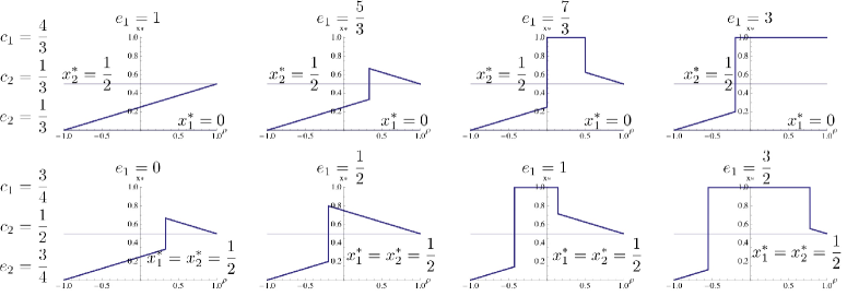
Figure 2: Impact of value correlation $(\rho)$ on bundle adoption $(x^{*})$ for different technology combinations (discrete model).

The impact of $\rho$ is illustrated in Fig. 2 that plots as a function of $\rho\in[-1,1]$, the adoption level of a technology bundle for different instances of the two above scenarios under the discrete correlation model of Section 5.

Specifically, the upper part of Fig. 2 displays adoption levels when bundling two heterogeneous technologies. Technology $1$ has a high cost, $c_{1}=4/3,$ which prevents it from taking off on its own, i.e., its stand-alone adoption remains at $x_{1}^{*}=0$, irrespective of its externality factor $e_{1}$. Technology $2$ has a low cost, $c_{2}=1/3,$ but marginal externality, $e_{2}=1/3,$ so that $x_{2}^{*}=1/2$. Combining the two technologies can benefit both, but only when the externality $e_{1}$ of technology $1$ is high enough, i.e., $e_{1}\geq 5/3$ (three right most plots). When $e_{1}$ is low, i.e., $e_{1}\leq 1$, technology $1$ still benefits from being bundled with technology $2$, but the reverse is not true $(x^{*}\leq 1/2)$. More interesting though than the impact of $e_{1}$ in creating a $WW$ outcome, is the role of $\rho$.

Specifically, when $e_{1}$ is large enough, the benefits of bundling arise only once $\rho$ exceeds a certain threshold. This is because early adopters of the bundle are driven primarily by the second technology, and under highly negative correlation in technology valuations, the first technology contributes added cost but little or no added value to those early adopters. Hence, adoption stops quickly at a level below that of the second technology offered alone. As correlation increases, the number of early adopters that derive positive utility from adopting the bundle increases to a point where adoption can reach enough of a critical mass to allow the externality effect of the first technology to become effective. This allows adoption to increase beyond what the second technology alone would have realized.

Note though that further increases in correlation need not yield additional improvements. As a matter of fact, increasing $\rho$ beyond the threshold can lower adoption (second plot from the left, $e_{1}=5/3$). This is because as correlation increases, the potential adoption “base” of the bundle narrows (both technologies appeal to an increasingly similar set of users), which limits the adoption equilibrium that can be reached. This effect persists until the externality factor of technology $1$ is strong enough to allow the bundle to reach full adoption (third and fourth plots from the left for $e_{1}=7/3,3$). As the externality factor of technology $1$ continues increasing, its strength becomes sufficient to preserve full adoption for some range of $\rho$ beyond the initial threshold. Further increases of $\rho$ outside that range can, however, result in the adoption level of the bundle dropping again (third plot from the left, $e_{1}=7/3$). This is only avoided once the externality factor of the first technology is strong enough that the range of $\rho$ values for which no decline in bundle’s adoption occurs extends all the way to $\rho=1$ (right-most plot for $e_{1}=3$).

Conversely, the lower part of Fig. 2 considers the bundling of two “middling” technologies, which alone only realize a relatively low adoption level $x_{1}^{*}=x_{2}^{*}=1/2$. They both have reasonably low costs, $c_{1}=3/4,c_{2}=1/2$, and can benefit from bundling when their combined externality factor, $e=e_{1}+e_{2}$ is high enough. The four plots display (left to right) adoption as a function of $\rho$ and for increasing values of $e$ ($e_{2}=3/4$ and $e_{1}$ varies from $0$ to $3/2$). They offer a qualitatively similar behavior as the upper part of Fig. 2, albeit with a more limited range, e.g., $WL$ outcomes can be eliminated (if $\rho$ is high enough) and decreases in adoption as $\rho$ keeps increasing cannot be avoided. This is not unexpected since the constraint that $x_{1}^{*}=x_{2}^{*}=1/2$ limits the range of costs and externality factors permissible.

In the next section, we explore the extent to which the above conclusions remain qualitatively valid under the more general model of continuous affinities of Section 4.

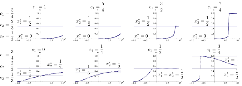
Figure 3: Impact of value correlation $(\rho)$ on bundle adoption $(x^{*})$ for different technology combinations (continuous model).

6.2 On the role of correlation (continuous model)

The discrete affinity model of Section 5 let us explicitly account for the impact of correlation when bundling services. Its relative simplicity, however, raises the question of whether the findings hold under more general (realistic) assumptions. An exhaustive assessment is clearly impractical, and we limit ourselves to the uniform distribution of Section 4 to offer initial evidence of the “robustness” of the results. Because, as mentioned in Section 4.5, an analytical investigation of uniformly distributed affinities under general correlation is complex, we resort to a numerical approach. Specifically, we consider a pair of bundling scenarios similar to those of Fig. 2, and numerically evaluate the bundle’s adoption for different values of $\rho$. The results are reported in Fig. 3, which largely mirrors Fig. 2 with some differences as we briefly review.

The two sets of plots in Fig. 3 clearly display the presence of a threshold effect, where correlation $(\rho)$ needs to exceed a certain minimum value before bundling becomes beneficial. This is particularly so when combining two heterogeneous services; a high-cost, high-externality one with a low-cost, low-externality one (top set of plots). Unlike the corresponding scenario in Fig. 2, the jump in the bundle’s adoption that occurs after crossing the threshold is not followed by a decline in adoption as $\rho$ further increases. This is likely because under a uniform distribution, the relative value of the externality after crossing the threshold is sufficient to prevent declines in adoption for larger values of $\rho$, i.e., a scenario similar to that of the top right-most plot of Fig. 2. The potentially negative impact of further increases in $\rho$ (beyond the threshold) is, however, seen in the lower set of plots of Fig. 3. In particular, the right-most plot clearly displays that while $\rho$ needs to exceed a threshold value of about $-0.4$ for the bundle to jump to full adoption $(x^{*}=1)$, increasing $\rho$ beyond this value results in progressively lower adoptions levels.

We note that the last scenario is an instance of a $SW$ rather than a true $WW$ scenario, and under continuous affinity distributions we did not identify instances of true $WW$ outcomes that exhibited a decline in adoption as $\rho$ increased beyond its “threshold” value. This is not unexpected, since as mentioned earlier, the shape of the joint distribution and not just the correlation coefficient is expected to affect the outcome. Hence, as distributions change, so will the exact configurations under which different effects arise as well as their magnitude. However, we believe that the general insight articulated in the previous section still holds, namely, the presence of a minimum correlation value to realize the critical mass of early adopters that a bundle with a high externality factor needs to succeed, and the fact that increasing $\rho$ beyond this value can narrow the bundle’s ultimate user base and, therefore, lower overall adoption unless its externality factor is large enough.

6.3 Summary

Based on the above results, the following bundling guidelines emerge to assist in identifying services, which, if bundled, can result in $WW$ outcomes:

Bundling guidelines: When bundling network services so as to bolster their adoption, it is best to choose services that are

1. 1. either heterogeneous in their cost-benefit structure, i.e., low cost & externality vs. high cost & externality,

   2. or of average cost and externality,

2. and sufficiently correlated in how users value them, but not too much.

The first guideline highlights that successful bundling outcomes require both a high overall externality factor, and a low enough cost to allow the creation of a sufficient critical mass of early adopters so that the value of the high externality can start being realized. The second guideline states that creating a sufficient critical mass of early adopters requires a certain minimum level of correlation in how users value the bundled services, but that once this level has been reached there is no benefit in selecting services that exhibit higher levels of correlation (and there could be disadvantages).

7 Conclusion

The paper presents an initial investigation aimed at developing a better understanding of when bundling networking technologies or services can be beneficial, i.e., result in higher adoption levels than when they are offered separately.

The question is of relevance in many practical settings as networking technologies commonly face early adoption hurdles until they acquire a large enough user-base to start delivering sufficient value. Bundling technologies can offer an effective solution to overcome those early adoption challenges, but it is often hard to predict whether it will succeed or not. Of particular importance in determining the outcome is correlation in how users value the individual technologies being bundled. The paper proposes simple models that can help explore this question in a principled manner, and illustrates the type of insight they provide through a few simple examples.

There are obviously many extensions that are desirable to the basic models described in the paper and in their ability to realistically capture how technologies interact, e.g., the extent to which they are complements or substitutes, or whether they exhibit economies of scope. The methodology outlined in the paper, however, offers a first step towards developing a fundamental understanding of the role that bundling can play in helping network technologies overcome initial adoption hurdles.

8 Acknowledgements

The authors wish to acknowledge the support of the National Science Foundation through award CNS-1116039. The contents of this paper belong to the authors and do not necessarily reflect the views of the National Science Foundation. The authors also wish to acknowledge helpful discussions with Kartik Hosanagar.

APPENDIX

A.1 Generating and characterizing correlated random variables

The generation of a pair of correlated uniform random variables $(U_{1},U_{2})$ is based on the following proposition.

Proposition A.1 ([Pearson (1907), Hotelling and Pabst (1936)]).

Let $(Z_{1},Z_{2})$ be a pair of independent standard normal RVs and fix $\rho\in[-1,1]$. Then

$$\left[\begin{array}[]{c}Y_{1}\\ Y_{2}\end{array}\right]=\left[\begin{array}[]{cc}Z_{1}&Z_{2}\end{array}\right]\left[\begin{array}[]{cc}1&\rho\\ 0&\sqrt{1-\rho^{2}}\end{array}\right]=\left[\begin{array}[]{c}Z_{1}\\ \rho Z_{1}+\sqrt{1-\rho^{2}}Z_{2}\end{array}\right]$$ (17)

are standard normal RVs with correlation $\rho$. Further, $U=(U_{1},U_{2})$ with $U_{i}=F_{Z}(Y_{i})$ for $i\in\{1,2\}$ are uniform RVs with correlation

$$\rho_{U}=\frac{6}{\pi}\sin^{-1}\left(\frac{\rho}{2}\right)\in[-1,1].$$ (18)

Remark A.2.

Selecting $\rho=2\sin(\pi\rho^{*}/6)$ for a target correlation $\rho^{*}$ ensures $\rho_{U}=\rho^{*}$. In what follows we will work with $\rho$ as the correlation parameter, even though $\rho_{U}$ is the actual correlation.

Remark A.3.

Observe $A=\left[\begin{array}[]{cc}1&\rho\\ 0&\sqrt{1-\rho^{2}}\end{array}\right]$ in Prop. A.1 is the Cholesky decomposition of the target correlation matrix $\Sigma=A^{\mathsf{T}}A=\left[\begin{array}[]{cc}1&\rho\\ \rho&1\end{array}\right]$.

From Prop. A.1 it is immediate to obtain the joint CDF on $(U_{1},U_{2})$ in terms of the correlation $\rho$, and from there the joint PDF.

Proposition A.4.

The joint CDF and joint PDF of $(U_{1},U_{2})$ in Prop. A.1 at $(u_{1},u_{2})$ are:

$$F_{U_{1},U_{2}}(u_{1},u_{2}) = \int_{0}^{u_{1}}F_{Z}\left(\frac{F_{Z}^{-1}(u_{2})-\rho F_{Z}^{-1}(v_{1})}{\sqrt{1-\rho^{2}}}\right)\mathrm{d}v_{1}$$ (19)

$$f_{U_{1},U_{2}}(u_{1},u_{2}) = \frac{1}{\sqrt{1-\rho^{2}}f_{Z}(F_{Z}^{-1}(u_{2}))}f_{Z}\left(\frac{F_{Z}^{-1}(u_{2})-\rho F_{Z}^{-1}(u_{1})}{\sqrt{1-\rho^{2}}}\right).$$ (20)

Proof A.5.

The joint CDF of $(U_{1},U_{2})$ at $(u_{1},u_{2})$ is:

$$F_{U_{1},U_{2}}(u_{1},u_{2}) = \mathbb{P}(U_{1}\leq u_{1},U_{2}\leq u_{2})$$ (21)

$$= \mathbb{P}(F_{Z}(Z_{1})\leq u_{1},F_{Z}(\rho Z_{1}+\sqrt{1-\rho^{2}}Z_{2})\leq u_{2})$$

$$= \mathbb{P}(Z_{1}\leq F_{Z}^{-1}(u_{1}),\rho Z_{1}+\sqrt{1-\rho^{2}}Z_{2}\leq F_{Z}^{-1}(u_{2}))$$

$$= \int_{-\infty}^{F_{Z}^{-1}(u_{1})}\mathbb{P}(Z_{1}\leq F_{Z}^{-1}(u_{1}),\rho Z_{1}+\sqrt{1-\rho^{2}}Z_{2}\leq F_{Z}^{-1}(u_{2})|Z_{1}=z_{1})f_{Z}(z_{1})\mathrm{d}z_{1}$$

$$= \int_{-\infty}^{F_{Z}^{-1}(u_{1})}\mathbb{P}(\rho z_{1}+\sqrt{1-\rho^{2}}Z_{2}\leq F_{Z}^{-1}(u_{2}))f_{Z}(z_{1})\mathrm{d}z_{1}$$

$$= \int_{-\infty}^{F_{Z}^{-1}(u_{1})}F_{Z}\left(\frac{F_{Z}^{-1}(u_{2})-\rho z_{1}}{\sqrt{1-\rho^{2}}}\right)f_{Z}(z_{1})\mathrm{d}z_{1}$$

Change of variables from $z_{1}$ to $v_{1}=F_{Z}(z_{1})$ gives Eq. (19). Differentiation w.r.t. $(u_{1},u_{2})$ gives

$$\frac{\partial}{\partial u_{1}}F_{U_{1},U_{2}}(u_{1},u_{2}) = F_{Z}\left(\frac{F_{Z}^{-1}(u_{2})-\rho F_{Z}^{-1}(u_{1})}{\sqrt{1-\rho^{2}}}\right)$$ (22)

$$f_{U_{1},U_{2}}(u_{1},u_{2}) = \frac{1}{\sqrt{1-\rho^{2}}}f_{Z}\left(\frac{F_{Z}^{-1}(u_{2})-\rho F_{Z}^{-1}(u_{1})}{\sqrt{1-\rho^{2}}}\right)\frac{\mathrm{d}}{\mathrm{d}u_{2}}F_{Z}^{-1}(u_{2})$$

Applying the inverse function theorem gives the joint PDF in Eq. (20).

The joint PDF $f_{U_{1},U_{2}}(u_{1},u_{2})$ is illustrated in Fig. 4 for $\rho\in\pm\frac{1}{2}$. The following proposition shows that this joint distribution recovers the distributions of perfectly negatively correlated, independent, and perfectly positively correlated uniform random variables as $\rho\to\{-1,0,+1\}$, respectively.

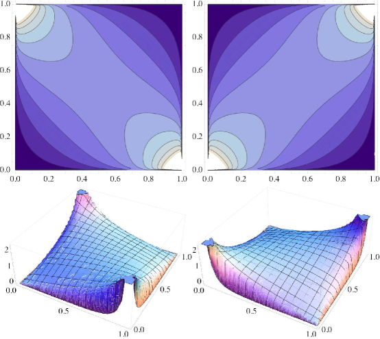
Figure 4: Contour plots (top) and 3-D plots (bottom) of the joint PDF on service affinities $f_{U_{1},U_{2}}(u_{1},u_{2})$ in Prop. A.4 for $\rho=-1/2$ (left) and $\rho=1/2$ (right).

Proposition A.6.

The limits of $F_{U_{1},U_{2}}(u_{1},u_{2})$ for $(u_{1},u_{2})\in[0,1]^{2}$ in Eq. (20) as $\rho\to\{-1,0,+1\}$ are

$$\lim_{\rho\to-1}F_{U_{1},U_{2}}(u_{1},u_{2}) = \max\{u_{1}+u_{2}-1,0\}$$

$$\lim_{\rho\to 0}F_{U_{1},U_{2}}(u_{1},u_{2}) = u_{1}u_{2}$$

$$\lim_{\rho\to 1}F_{U_{1},U_{2}}(u_{1},u_{2}) = \min\{u_{1},u_{2}\}$$ (23)

corresponding to $U_{1}+U_{2}=1$ (a.s.), $(U_{1},U_{2})$ independent, and $U_{1}=U_{2}$ (a.s.), respectively.

Proof A.7.

Since the integral is over a finite support and the integrand is continuous:

$$\lim_{\rho\to\pm 1}F_{U_{1},U_{2}}(u_{1},u_{2})=\int_{0}^{u_{1}}F_{Z}\left(\lim_{\rho\to\pm 1}\frac{F_{Z}^{-1}(u_{2})-\rho F_{Z}^{-1}(v_{1})}{\sqrt{1-\rho^{2}}}\right)\mathrm{d}v_{1}.$$ (24)

It follows that $F_{U_{1},U_{2}}(u_{1},u_{2})\to u_{1}u_{2}$ as $\rho\to 0$. Next, as $\rho\to 1$ observe as $u_{2}\gtrless v_{1}$ the function inside $F_{Z}(\cdot)$ in Eq. (24) goes to $\pm\infty$, respectively. Thus:

$$u_{1}<u_{2} \Rightarrow \lim_{\rho\to 1}F_{U_{1},U_{2}}(u_{1},u_{2})=\int_{0}^{u_{1}}F_{Z}(\infty)\mathrm{d}v_{1}=u_{1}$$

$$u_{1}>u_{2} \Rightarrow \lim_{\rho\to 1}F_{U_{1},U_{2}}(u_{1},u_{2})=\int_{0}^{u_{2}}F_{Z}(\infty)\mathrm{d}v_{1}+\int_{u_{2}}^{u_{1}}F_{Z}(-\infty)\mathrm{d}v_{1}=u_{2}$$ (25)

and so $\lim_{\rho\to 1}F_{U_{1},U_{2}}(u_{1},u_{2})=\min\{u_{1},u_{2}\}$. Finally, as $\rho\to-1$ observe as $F_{Z}^{-1}(u_{2})+F_{Z}^{-1}(v_{1})\gtrless 0$ the function inside $F_{Z}(\cdot)$ in Eq. (24) goes to $\pm\infty$, respectively. Observe

$$F_{Z}^{-1}(u_{2})+F_{Z}^{-1}(v_{1})\gtrless 0~{}\Leftrightarrow~{}F_{Z}^{-1}(u_{2})\gtrless F_{Z}^{-1}(1-v_{1})~{}\Leftrightarrow~{}v_{1}+u_{2}\gtrless 1.$$ (26)

Thus:

$$u_{1}+u_{2}\leq 1 \Rightarrow \lim_{\rho\to-1}F_{U_{1},U_{2}}(u_{1},u_{2})=\int_{0}^{u_{1}}F_{Z}(-\infty)\mathrm{d}v_{1}=0$$ (27)

$$u_{1}+u_{2}\geq 1 \Rightarrow \lim_{\rho\to-1}F_{U_{1},U_{2}}(u_{1},u_{2})=\int_{0}^{1-u_{2}}F_{Z}(-\infty)\mathrm{d}v_{1}+\int_{1-u_{2}}^{u_{1}}F_{Z}(\infty)\mathrm{d}v_{1}=u_{1}+u_{2}-1$$

and so $\lim_{\rho\to 1}F_{U_{1},U_{2}}(u_{1},u_{2})=\max\{u_{1}+u_{2}-1,0\}$.

The following two functions are central to the subsequent proposition.

$$\psi_{u,\rho}(v) \equiv F_{Z}\left(\frac{F_{Z}^{-1}(u-v)-\rho F_{Z}^{-1}(v)}{\sqrt{1-\rho^{2}}}\right)$$ (28)

$$\phi_{u,\rho}(v) \equiv f_{Z}\left(\frac{F_{Z}^{-1}(u-v)-\rho F_{Z}^{-1}(v)}{\sqrt{1-\rho^{2}}}\right)\frac{1}{f_{Z}(F_{Z}^{-1}(u-v))}$$ (29)

for $i)$ $u\in(0,2]$, $ii)$ $v\in[0,u]$ when $u\in(0,1]$ and $v\in[u-1,1]$ when $u\in(1,2]$, and $iii)$ $\rho\in[-1,1]$.

Proposition A.8.

The aggregate affinity under bundling $U=U_{1}+U_{2}$ has CDF

$$F_{U}(u)=\left\{\begin{array}[]{ll}\displaystyle\int_{0}^{u}\psi_{u,\rho}(v)\mathrm{d}v,&u\in(0,1]\\ \displaystyle\int_{u-1}^{1}\psi_{u,\rho}(v)\mathrm{d}v+u-1,&u\in[1,2]\end{array}\right.$$ (30)

and PDF

$$f_{U}(u)=\left\{\begin{array}[]{ll}\frac{1}{\sqrt{1-\rho^{2}}}\displaystyle\int_{0}^{u}\phi_{u,\rho}(v)\mathrm{d}v,&u\in(0,1]\\ \frac{1}{\sqrt{1-\rho^{2}}}\displaystyle\int_{u-1}^{1}\phi_{u,\rho}(v)\mathrm{d}v,&u\in[1,2]\end{array}\right.$$ (31)

for $\psi_{u,\rho}(v)$ in Eq. (28) and $\phi_{u,\rho}(v)$ in Eq. (29). Further, $F_{U}(1)=1/2$ for all $\rho$.

Proof A.9 (of Prop. A.8).

From Eq. (17), the CDF of $U=U_{1}+U_{2}$ in terms of the iid standard normal random variables $(Z_{1},Z_{2})$ and the correlation parameter $\rho$ is

$$F_{U}(u)=\mathbb{P}\left(F_{Z}(Z_{1})+F_{Z}\left(\rho Z_{1}+\sqrt{1-\rho^{2}}Z_{2}\right)\leq u\right).$$ (32)

For $u\in(0,1]$ condition on $z_{1}\in\mathbb{R}$, split the integral at $z_{1}=F_{Z}^{-1}(u)$, and note the event of interest cannot occur for $z_{1}>F_{Z}^{-1}(u)$:

$$F_{U}(u)=\int_{-\infty}^{F_{Z}^{-1}(u)}\mathbb{P}(F_{Z}(Z_{1})+F_{Z}(\rho Z_{1}+\sqrt{1-\rho^{2}}Z_{2})\leq u|Z_{1}=z_{1})f_{Z}(z_{1})\mathrm{d}z_{1}$$ (33)

Simplification gives the top equation in Eq. (35). For $u\in(1,2]$ condition on $z_{1}\in\mathbb{R}$, split the integral at $z_{1}=F_{Z}^{-1}(u-1)$ and notice the event of interest is assured for $z_{1}\leq F_{Z}^{-1}(u-1)$:

$$F_{U}(u)=F_{Z}(F_{Z}^{-1}(u-1))+\int_{F_{Z}^{-1}(u-1)}^{\infty}\mathbb{P}(F_{Z}(z_{1})+F_{Z}(\rho z_{1}+\sqrt{1-\rho^{2}}Z_{2})\leq u)f_{Z}(z_{1})\mathrm{d}z_{1}$$ (34)

Simplification gives the bottom equation in Eq. (35).

$$F_{U}(u)=\left\{\begin{array}[]{ll}\displaystyle\int_{-\infty}^{F_{Z}^{-1}(u)}F_{Z}\left(\frac{F_{Z}^{-1}(u-F_{Z}(z_{1}))-\rho z_{1}}{\sqrt{1-\rho^{2}}}\right)f_{Z}(z_{1})\mathrm{d}z_{1},&u\in(0,1]\\ u-1+\displaystyle\int_{F_{Z}^{-1}(u-1)}^{\infty}F_{Z}\left(\frac{F_{Z}^{-1}(u-F_{Z}(z_{1}))-\rho z_{1}}{\sqrt{1-\rho^{2}}}\right)f_{Z}(z_{1})\mathrm{d}z_{1},&u\in[1,2]\end{array}\right.$$ (35)

Change variables from $z_{1}$ to $v=F_{Z}(z_{1})$ to obtain Eq. (30).

Apply the Leibniz integral rule to differentiate $F_{U}(u)$ and apply the inverse function theorem. For $u\in[0,1]$:

$$f_{U}(u) = F_{Z}\left(\frac{F_{Z}^{-1}(u-u)-\rho F_{Z}^{-1}(u)}{\sqrt{1-\rho^{2}}}\right)+\int_{0}^{u}\frac{\mathrm{d}}{\mathrm{d}u}F_{Z}\left(\frac{F_{Z}^{-1}(u-v)-\rho F_{Z}^{-1}(v)}{\sqrt{1-\rho^{2}}}\right)\mathrm{d}v$$ (36)

$$= \frac{1}{\sqrt{1-\rho^{2}}}\int_{0}^{u}f_{Z}\left(\frac{F_{Z}^{-1}(u-v)-\rho F_{Z}^{-1}(v)}{\sqrt{1-\rho^{2}}}\right)\frac{1}{f_{Z}(F_{Z}^{-1}(u-v))}\mathrm{d}v$$

Change variables from $z_{1}$ to $v=F_{Z}(z_{1})$ to obtain the top equation in Eq. (31). Likewise, for $u\in(1,2]$:

$$f_{U}(u) = 1-F_{Z}\left(\frac{F_{Z}^{-1}(u-(u-1))-\rho F_{Z}^{-1}(u-1)}{\sqrt{1-\rho^{2}}}\right)+$$ (37)

$$\int_{u-1}^{1}\frac{\mathrm{d}}{\mathrm{d}u}F_{Z}\left(\frac{F_{Z}^{-1}(u-v)-\rho F_{Z}^{-1}(v)}{\sqrt{1-\rho^{2}}}\right)\mathrm{d}v$$

$$= \frac{1}{\sqrt{1-\rho^{2}}}\int_{u-1}^{1}f_{Z}\left(\frac{F_{Z}^{-1}(u-v)-\rho F_{Z}^{-1}(v)}{\sqrt{1-\rho^{2}}}\right)\frac{1}{f_{Z}(F_{Z}^{-1}(u-v))}\mathrm{d}v$$

Change variables from $z_{1}$ to $v=F_{Z}(z_{1})$ to obtain the bottom equation in Eq. (31).

Finally, we show $F_{U}(1)=1/2$ for all $\rho$. Observe $F_{Z}^{-1}(1-v)=-F_{Z}^{-1}(v)$ and thus

$$F_{U}(1)=\int_{0}^{1}F_{Z}\left(\frac{F_{Z}^{-1}(1-v)-\rho F_{Z}^{-1}(v)}{\sqrt{1-\rho^{2}}}\right)\mathrm{d}v=\int_{0}^{1}F_{Z}\left(-F_{Z}^{-1}(v)\sqrt{\frac{1+\rho}{1-\rho}}\right)\mathrm{d}v.$$ (38)

Set $a=-\sqrt{(1+\rho)/(1-\rho)}$ and write the last expression above as

$$g_{1}(a)=\int_{0}^{1}F_{Z}(aF_{Z}^{-1}(v))\mathrm{d}v=\int_{-\infty}^{\infty}F_{Z}(az)f_{Z}(z)\mathrm{d}z,$$ (39)

using the change of variable $z=F_{Z}^{-1}(v)$. The derivative w.r.t. $a$ is

$$g_{1}^{\prime}(a)=\int_{-\infty}^{\infty}zf_{Z}(az)f_{Z}(z)\mathrm{d}z=\int_{-\infty}^{\infty}g_{2}(z,a)\mathrm{d}z,$$ (40)

for $g_{2}(z,a)\equiv zf_{Z}(az)f_{Z}(z)$. Now observe $g_{2}(z,a)=-g_{2}(-z,a)$, i.e., $g_{2}(z,a)$ is an odd function in $z$ for all $a$, and thus $g_{1}^{\prime}(a)=0$, and $g_{1}(a)$ is a constant for all $a$. Using the change of variable $u=F_{Z}(z)$ at $a=1$ gives

$$g_{1}(1)=\int_{0}^{1}u\mathrm{d}u=\frac{1}{2}.$$ (41)

Thus $F_{U}(1)=1/2$ for all $\rho$.

Representative plots of the CDF and PDF for $U$ in Prop. A.8 are shown in Fig. 5.

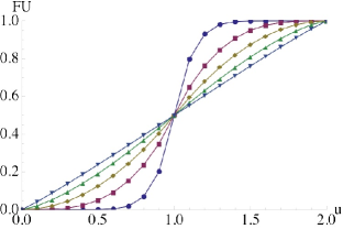
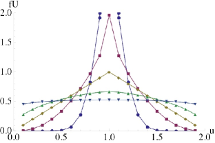
Figure 5: The CDF (left) and PDF (right) for the aggregate affinity $U=U_{1}+U_{2}$ from Prop. A.8 for $\rho\in\{-0.9,-0.5,0,0.5,0.9\}$.

Remark A.10.

The standard tool to construct a joint distributions with specified marginals is the copula [Nelsen (2009)]. In our context, a copula would specify a joint distribution on $[0,1]^{2}$ with uniform marginals on $[0,1]$. Although there are many copulas that handle this quite easily, our requirements are a bit specific in that we desire $i)$ to directly parameterize the correlation of the joint distribution, and $ii)$ to have a “simple” distribution for the sum $U=U_{1}+U_{2}$. Although the construction we have employed falls short of this second objective in that $F_{U}$ is expressible only in terms of an integral, nonetheless our preliminary investigation into copulas has not identified a candidate family of copulas meeting both objectives.

Remark A.11.

Correlation is not in general a sufficient parameter to completely capture the dependence of the adoption level on the joint distribution. In fact we expect that the adoption levels of two joint distributions on $[0,1]^{2}$ with uniform marginals and common correlation may have distinct adoption levels, precisely because the solution of $h(x)=x$ depends upon the distribution of the aggregate affinity, $F_{U}$. Nonetheless, we view the correlation parameter as an insightful knob to vary in order to highlight the fact that the adoption level is quite sensitive to the joint distribution of the affinities.

A.2 Separate adoption equilibria under uniformly distributed user affinities

Proposition 4.1 characterized the possible equilibria for separate service offerings when the user service affinities are uniform random variables. The results are illustrated in Fig. 6.

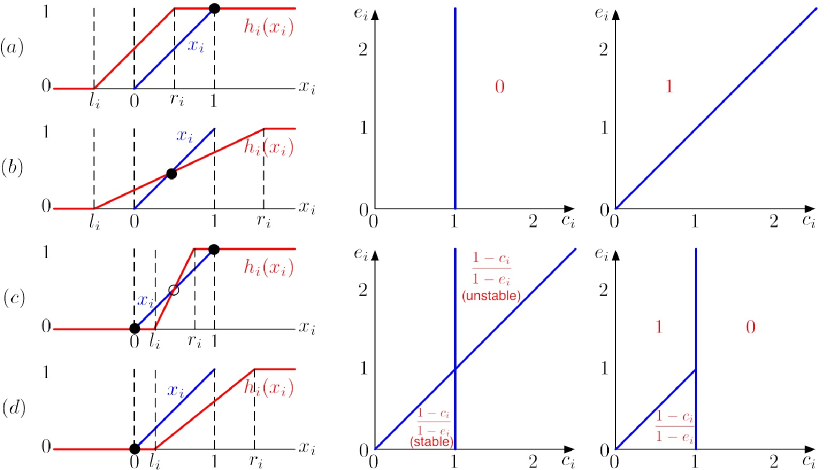
Figure 6: Illustration of Prop. 4.1. Equilibria adoption levels for continuous affinities with separate service offerings. Equilibria $x_{i}^{*}\in[0,1]$ solve $h_{i}(x_{i})=x_{i}$, where $h_{i}(x_{i})$ has thresholds $l_{i},r_{i}$. The left figure shows the four orderings $(a)$ $l_{i}<0<r_{i}<1$, $(b)$ $l_{i}<0<1<r_{i}$, $(c)$ $0<l_{i}<r_{i}<1$, and $(d)$ $0<l_{i}$ and $1<r_{i}$, with black (open) dots indicating stable (unstable) equilibria. The possible equilibria are $0,1,(1-c_{i})/(1-e_{i})$. The first three subfigures of the right figure show the $(c_{i},e_{i})$ plane and the regions for which each of the three equilibria are found. The final subfigure on the bottom right shows a partition of the $(c_{i},e_{i})$ plane in terms of the lowest possible stable equilibria.

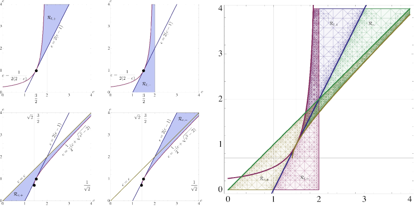
Figure 7: The four equilibria regions $\mathcal{R}_{l,\pm},\mathcal{R}_{r,\pm}$ of the $(c,e)$ plane in Eq. (4.4) for continuous and independent affinities $(U_{1},U_{2})$.

A.3 Bundle adoption equilibria under continuous users affinity distributions

Proposition A.12.

The probability of bundle adoption $h(x)$ in Eq. (4) at adoption level $x$ for aggregate continuous affinity $U$ from Prop. A.8 is

$$h(x)=\left\{\begin{array}[]{lrcccl}0,&&&x&\leq&l\\ 2-(c-ex)-\displaystyle\int_{c-ex-1}^{1}F_{Z}\left(\frac{F_{Z}^{-1}(c-ex-v)-\rho F_{Z}^{-1}(v)}{\sqrt{1-\rho^{2}}}\right)\mathrm{d}v,&l&<&x&\leq&m\\ 1-\displaystyle\int_{0}^{c-ex}F_{Z}\left(\frac{F_{Z}^{-1}(c-ex-v)-\rho F_{Z}^{-1}(v)}{\sqrt{1-\rho^{2}}}\right)\mathrm{d}v,&m&<&x&\leq&r\\ 1,&r&<&x&&\end{array}\right.,$$ (42)

for adoption thresholds $l\equiv\frac{c-2}{e}$, $m\equiv\frac{c-1}{e}$, and $r\equiv\frac{c}{e}$. The function $h(x)$ has the following properties:

1. $h^{\prime}(x)=ef_{U}(c-ex)\geq 0$

2. $h^{{}^{\prime\prime}}(x)=-e^{2}f_{U}^{\prime}(c-ex)$

3. $h(m)=\frac{1}{2}$

Stable equilibria include $x^{*}\in\{0,1\}$, where $x^{*}=0$ is an equilibrium provided $h(0)=0\Leftrightarrow c>2$, and $x^{*}=1$ is an equilibrium provided $h(1)=1\Leftrightarrow c<e$.

Proof A.13.

Eq. (42) is immediate from the definition $h(x)=\mathbb{P}(U>c-ex)$ in Eq. (4) and Prop. A.8. The first two properties are immediate from the definition of $h(x)$ and the fact that the CDF of $U$ is differentiable, by assumption. The property $h(m)=1/2$ follows immediately from $F_{U}(1)=1/2$ in Prop. A.8.

As stated in Corollary 4.4, bundle adoption equilibria satisfy $h(x)=x$ with solutions given by Eq. (11).

The regions in Eq. (4.4) are illustrated in Fig. 7, which illustrates their shape. Observe $i)$ $e=2(c-1)$ is the solution of $\xi_{l,\pm}^{*}=m$ and $\xi_{r,\pm}^{*}=m$, $ii)$ $e=1/(2(2-c))$ is the solution of $2(c-2)e+1=0$ where $2(c-2)e+1$ is the discriminant of $\xi_{l,\pm}^{*}$ in Eq. (11), and $iii)$ $e=\frac{1}{2}(c+\sqrt{c^{2}-2})$ is the solution of $2(e-c)e+1=0$ where $2(e-c)e+1$ is the discriminant of $\xi_{r,\pm}^{*}$ in Eq. (11).

A.4 Separate adoption equilibria under discrete user affinities

Fig. 8 illustrates possible adoption equilibria under discrete user affinities, and the regions of the $(c_{i},e_{i})$ plane they correspond to.

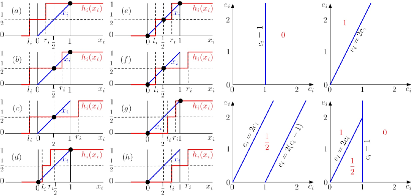
Figure 8: Illustration of Prop. 5.1. Left: the eight possible orderings of $\{l_{i},r_{i}\}$ with $\{0,1/2,1\}$ each determine the subset of $\{0,1/2,1\}$ that are equilibria. All equilibria are stable. Right: the $(c_{i},e_{i})$ plane and the equilibria in each region. Bottom right: partition of the $(c_{i},e_{i})$ plane according to lowest stable equilibria.

A.5 Bundle adoption equilibria under discrete user affinities

Fig. 9 parallels Fig. 8, and illustrates Prop. 5.2. Of interest is comparing the bottom-right plots of Fig. 8 and Fig. 9, to identify the regions where bundling yields a higher adoption equilibrium. Different regions, and therefore outcomes arise as $\rho$ varies.

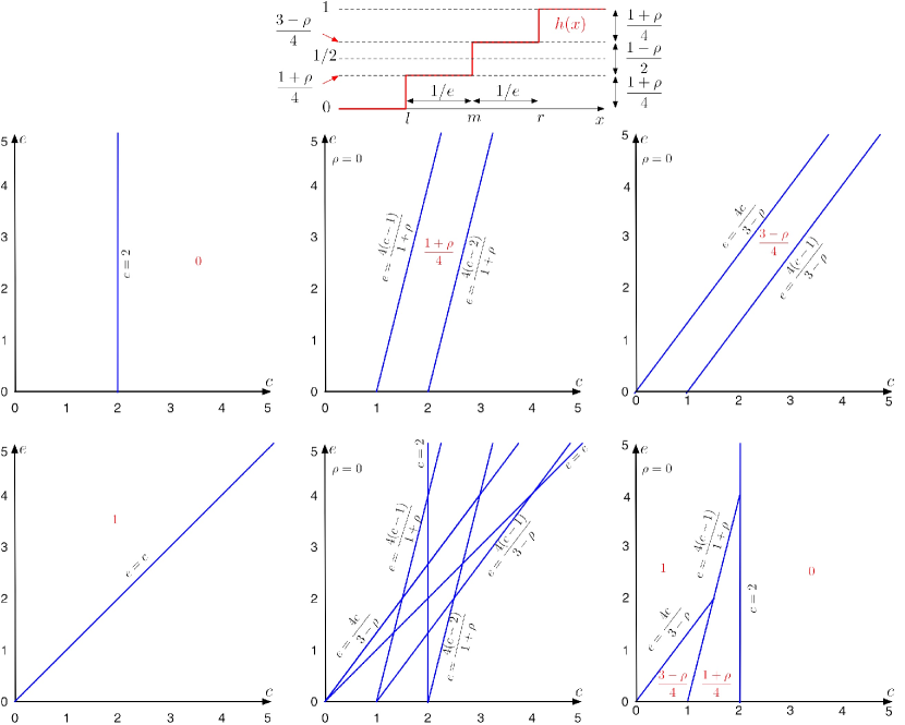
Figure 9: Illustration of Prop. 5.2. Top: the probability of adoption $h(x)$ in Eq. (13) in terms of $p$ (left) and $\rho$ (right). Bottom: the regions of the $(c,e)$ plane for each of the four equilibria $\{0,(1+\rho)/4,(3-\rho)/4,1\}$. Also shown are the superimposed boundaries of the four equilibria regions, as well as the partition of the $(c,e)$ plane according to the lowest stable equilibria. The figures are shown for $\rho=0$.

References

- [1]
- Arthur (2013) C. Arthur. 2013. NSA scandal: what data is being monitored and how does it work? The Guardian. (2013). Available at http://www.guardian.co.uk/world/2013/jun/07/nsa-prism-records-surveillance-questions.
- Bakos and Brynjolfsson (1999) Y. Bakos and E. Brynjolfsson. 1999. Bundling Information Goods: Pricing, Profits, and Efficiency. Management Science 45, 12 (December 1999).
- Bhargava and Choudhary (2004) H. K. Bhargava and V. Choudhary. 2004. Economics of an information intermediary with aggregation benefits. Information Systems Research. 15, 1 (2004), 22–36.
- Brewster (2013) T. Brewster. 2013. Tor network spike caused by botnet. TechWeekEurope. (September 2013). Available at http://www.techweekeurope.co.uk/news/mevade-botnet-tor-network-126497.
- Cabral (1990) L.M.B. Cabral. 1990. On the adoption of innovation with network externalities. Mathematical Social Sciences 19 (1990), 299–308.
- Chao and Derdenger (2013) Y. Chao and T. Derdenger. 2013. Mixed bundling in two-sided markets in the presence of installed base effects. Management Science 57, 3 (March 2013).
- Fernández Franco (2012) L. Fernández Franco. 2012. A survey and comparison of anonymous communication systems: Anonymity and security. Universitat Oberta de Catalunya - Institutional Repository. (June 2012). Available at http://hdl.handle.net/10609/14740.
- Fudenberg and Tirole. (1991) D. Fudenberg and J. Tirole. 1991. Game Theory. MIT Press., Cambridge, MA.
- Hotelling and Pabst (1936) H. Hotelling and M.R. Pabst. 1936. Rank correlation and tests of significance involving no assumption of normality. The Annals of Mathematical Statistics 7 (1936), 29–43.
- McAfee et al. (1989) R.P. McAfee, J. McMillan, and M.D. Whinston. 1989. Multiproduct Monopoly, Commodity Bundling, and Correlation of Values. The Quarterly Journal of Economics 104, 2 (May 1989).
- Nelsen (2009) R.B. Nelsen. 2009. An introduction to copulas (second ed.). Springer.
- Ozment and Schechter (2006) A. Ozment and S.E. Schechter. 2006. Bootstrapping the adoption of Internet security protocols. In Proc. WEIS.
- Pang and Etzion (2012) M.-S. Pang and H. Etzion. 2012. Analyzing pricing strategies for online services with network effects. Information Systems Research 23, 4 (December 2012).
- Pearson (1907) K. Pearson. 1907. On further methods of determining correlation. Drapers’ Company Research Memoirs Biometric Series IV (1907).
- Peres et al. (2010) R. Peres, E. Muller, and V. Mahajan. 2010. Innovation diffusion and new product growth models: A critical review and research directions. International Journal of Research in Marketing 27 (2010).
- Prasad et al. (2010) A. Prasad, R. Venkatesh, and V. Mahajan. 2010. Optimal bundling of technological products with network externality. Management Science 56, 12 (December 2010).
- Schmalensee (1984) R. Schmalensee. 1984. Gaussian Demand and Commodity Bundling. Journal of Business 57, 1 (1984).
- Venkatesh and Mahajan (2009) R. Venkatesh and V. Mahajan. 2009. The design and pricing of product bundles: A review of normative guidelines and practical approaches. In Handbook of Pricing Research in Marketing, V.R. Rao (Ed.). Edward Elgar Publishing, 232–257.