Update on the Sea Contributions to Hadron Electric Polarizabilities through Reweighting

Abstract:

We present the results of a reweighting calculation to compute the contribution of the charged quark sea to the neutron electric polarizability. The chief difficulty is the stochastic estimation of weight factors, and we present a hopping parameter expansion-based technique for reducing the stochastic noise, along with a discussion of why this particular reweighting is so difficult. We used this technique to estimate weight factors for 300 configurations of nHYP-clover fermions and compute the neutron polarizability, but the reweighting greatly inflates the overall statistical error, driven by the stochastic noise in the weight factors.

1 Introduction

At leading order, the interaction of hadrons with a background electromagnetic field can be parametrized by a variety of electromagnetic polarizabilities which characterize the deformation of the hadron by the field. Of these, the electric polarizability $\alpha$ describes the induced dipole by an external static, uniform electric field. It is defined as the ratio of the electric field and the induced dipole moment: $\alpha=\bf d/\bf E$. Since lattice QCD is best able to measure spectroscopic information, we attack the polarizability through the induced interaction energy $\delta E=-\frac{1}{2}\alpha E^{2}$.

A lattice calculation of the neutron electric polarizability is desirable for three reasons. First, the experimental uncertainties in these quantities are still over $10\%$, and it may be the case that ultimately the lattice can provide an improvement in the ultimate precision of this quantity. Second, if lattice QCD is to be considered a successful approach to simulating the hadronization of quarks and their properties, then the measurement of such a fundamental property of the neutron is something of a basic test. Finally, the flexibility of lattice calculations (the freedom to use nonphysical parameters) may provide some insight into the origins of the neutron polarizability. The first lattice study of the neutron polarizability was done in 1989 [1], on a $10^{3}\times 20$ quenched lattice with $a\simeq 0.11$ fm using unimproved staggered fermions; this study and a subsequent early study using both Wilson and clover fermions on a quenched sea [2], show good agreement with the experimental value.

More recently, calculations using dynamical quarks and larger lattices have produced values that are substantially smaller, suggesting that the early agreement with experiment was a lucky accident [3, 4, 5]. Clearly the simulations differ from the physical limit in some crucial manner and thus fail to reproduce the neutron polarizability. Here we are concerned with potentially the most difficult effect: the interactions between the electric field and the sea quarks.

1.1 The background field method

Since the ground state energy of the neutron is shifted by an amount $\Delta E=-\frac{1}{2}\alpha E^{2}$ in an external electric field, spectroscopic measurements on the lattice can provide a direct avenue to access the polarizability. One simply measures the neutron mass with the background field and without it, then computes $\Delta E$. We choose to use Dirichlet boundary conditions in time and in the direction of the electric field. While this means that we have no true zero-momentum state, this can be treated as but an additional finite-size effect whose effect can be partially compensated for but which will in any case go away in the infinite-volume limit. This is preferable to the uncontrolled finite-size effects associated with the electric field with periodic boundary conditions.

We parametrize the electric field with the dimensionless parameter $\eta\equiv a^{2}qE$ and choose a gauge such that

$$U_{4}\rightarrow U_{4}e^{i\eta x/a}.$$ (1)

In Euclidean time this corresponds to an imaginary $E$ field, but as detailed in [5] the result can be analytically continued to real $E$ without issue.

The energy shift caused by the external electric field is quite small, smaller than the error in $M_{N}$ itself. Thus, in order to resolve it, we must take into account the fact that the correlators measured with and without the electric field are strongly correlated, and only become more strongly correlated as the strength of the electric field is decreased. To fit the nucleon correlators, we construct a covariance matrix including “cross terms” which give the mixed covariance between zero-field and nonzero-field correlators. We then fit all the data at once, using the fit form

$$G(t,\eta)=(A+B\eta^{2})e^{-(M_{N}+C\eta^{2})t}$$ (2)

to extract $M_{N}$ and the parameter $C$ which is related to $\alpha$. (Contributions linear in $\eta$ are zero due to reflection symmetry in the gauge average.)

1.2 Reweighting

The simplest way to incorporate the effect of the electric field on the sea quarks would be to include its effects in gauge generation where the sea dynamics are simulated. However, generating a separate Monte Carlo ensemble to compute the correlator in the presence of background field would ruin the correlations which are necessary to achieve a small overall error. Thus, we turn to reweighting as a method of creating two ensembles which have different sea-quark actions yet are correlated. A similar approach has been used before to compute the strangeness of the nucleon using the Feynman-Hellman theorem [6], which requires a measurement of ${{\partial M_{N}}\over{\partial m_{s}}}$.

Since the contribution of the $U(1)$ field to the gauge action is independent of the gauge links, it cancels, and the weight factor is the standard ratio of fermion determinants $w_{i}={\det{\bf M_{E}}/\det{\bf M_{0}}}$.

We want to include the effect of the electric field on both sea quark flavors; this can be done by simply computing weight factors at the two values of $\eta$ corresponding to the quark charges and multiplying them. The chief difficulty in this calculation is that the determinant ratio must be estimated stochastically, and this is far more difficult than for mass reweighting [7]. Even if the fluctuations in the weight factor are small in absolute magnitude, the size of the error is governed by the correlation between zero and nonzero field correlators. As this correlation is strong and becomes stronger as $\eta\rightarrow 0$, reweighting the latter but not the former may substantially reduce the strength of this correlation even if the weight factors are all very close to unity.

2 Simulation details

We performed this reweighting calculation on a $24^{3}\times 48$ ensemble of 300 minimally-correlated gauge configurations using two dynamical flavors of nHYP-smeared Wilson-clover fermions [8] and a standard Symanzik-improved gauge action. The lattice spacing was $a\approx 0.126$ fm, determined by fitting the static quark potential to determine the Sommer scale $r_{1}$[9]. We used $\kappa=0.1282$ for the dynamical quarks, corresponding to $m_{\pi,{\mathrm{s}ea}}\approx 300$ MeV.

3 Stochastic estimators for the weight factor

The standard stochastic estimator for the determinant ratio is

$$w_{i}=\left\langle e^{-\xi^{\dagger}(\Omega-1)\xi}\right\rangle_{e^{-\xi^{\dagger}\xi}}$$ (3)

where $\Omega=\bf M_{E}^{-1}\bf M_{0}$ [10]. However, this stochastic estimator has very large fluctuations in the present case, and neither of the improvement techniques that has been shown to be successful for mass reweighting is successful here [7].

3.1 Pseudo-perturbative estimator

We thus turn to a pseudo-perturbative estimate of the weight factor, in which we estimate not the weight factor itself but its first and second derivatives with respect to $\eta$ for a single quark flavor, allowing us to construct the weight factor at any given $\eta$ by a power series. Such an expansion is appropriate since we are explicitly unconcerned with higher order effects. These derivatives can be expressed as the traces of combinations of operators [7]:

$$\left.{{\partial}\over{\partial\eta}}\frac{\det M_{\eta}}{\det M}\right|_{\eta=0} ={\rm Tr\,}\left({{\partial M}\over{\partial\eta}}M^{-1}\right)$$ (4)

$$\left.{{\partial^{2}}\over{\partial\eta}^{2}}\frac{\det M}{\det M}\right|_{\eta=0} ={\rm Tr\,}\left({{\partial^{2}M}\over{\partial\eta}^{2}}M^{-1}\right)-{\rm Tr\,}\left({{\partial M}\over{\partial\eta}}M^{-1}{{\partial M}\over{\partial\eta}}M^{-1}\right)+\left[{\rm Tr\,}\left({{\partial M}\over{\partial\eta}}M_{0}^{-1}\right)\right]^{2}$$ (5)

These traces still must be estimated stochastically; this is done with the standard estimator ${\rm Tr\,}\mathcal{O}=\left\langle\xi^{\dagger}\mathcal{O}\xi\right\rangle$, where we use $Z(4)$ noises for $\xi$.

3.2 Hopping parameter improvement

This stochastic estimator can be further improved using an improvement technique. If other operators $\mathcal{O}^{\prime}_{i}$ can be identified such that the stochastic fluctuations in $\xi^{\dagger}\mathcal{O}\xi$ and $\xi^{\dagger}\mathcal{O}^{\prime}_{i}\xi$ are correlated, then we can reduce the overall fluctuations by writing

$${\rm Tr\,}\mathcal{O}=\left\langle\xi^{\dagger}\left(\mathcal{O}-\sum_{i}\mathcal{O}^{\prime}_{i}\right)\xi\right\rangle+\sum_{i}{\rm Tr\,}\mathcal{O}^{\prime}_{i}.$$ (6)

For the operators here, we can expand each occurrence of $M^{-1}$ in powers of $\kappa$, with each order in the expansion acting as one of the $\mathcal{O}^{\prime}_{i}$’s. The leading terms in the HPE approximate the near-diagonal behavior of the operators, and the variance in the stochastic estimate of ${\rm Tr\,}\mathcal{O}$ is equal to the sum of all off-diagonal elements of $\mathcal{O}$. By subtracting an approximation of these terms from the estimator the variance can be reduced [11]. The exact traces of these operators can be calculated analytically since they consist of finite numbers of hops [7]; we have computed them up to $7^{\mathrm{th}}$ order in $\kappa$. The reduction in the variance can be calculated to much higher order; it is shown in Fig. 1.

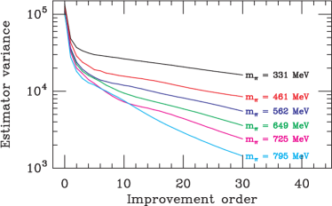
Figure 1: Improvement in the variance of the stochastic estimator of ${{\partial w}\over{\partial\eta}}$ as a function of the order of the hopping parameter expansion for different values of $m_{\pi}$, computed from 100 stochastic estimates for each $\kappa$.

3.3 The origin of the noise

The estimator noise on ${\rm Tr\,}\mathcal{O}$ is proportional to the sum in quadrature of off-diagonal elements in $\mathcal{O}$. While computing all of these elements is even more impractical than a complete computation of the trace, we can map a representative set of them to understand the origin of the estimator noise and see the effect of the HPE procedure on reducing it. This is shown in Fig. 2 for the first-order term, $\mathcal{O}={{\partial M}\over{\partial\eta}}M^{-1}$. Here we see the origin of the huge estimator noise: the diagonal elements are dwarfed by the near-diagonal noise contributions. This is in contrast to $M^{-1}$ alone, which is diagonal dominant and where the estimator converges nicely in a handful of noises. As expected, the HPE improvement suppresses, but does not eliminate, off-diagonal contributions within a Manhattan distance equal to the HPE order, and does not affect those outside this range.

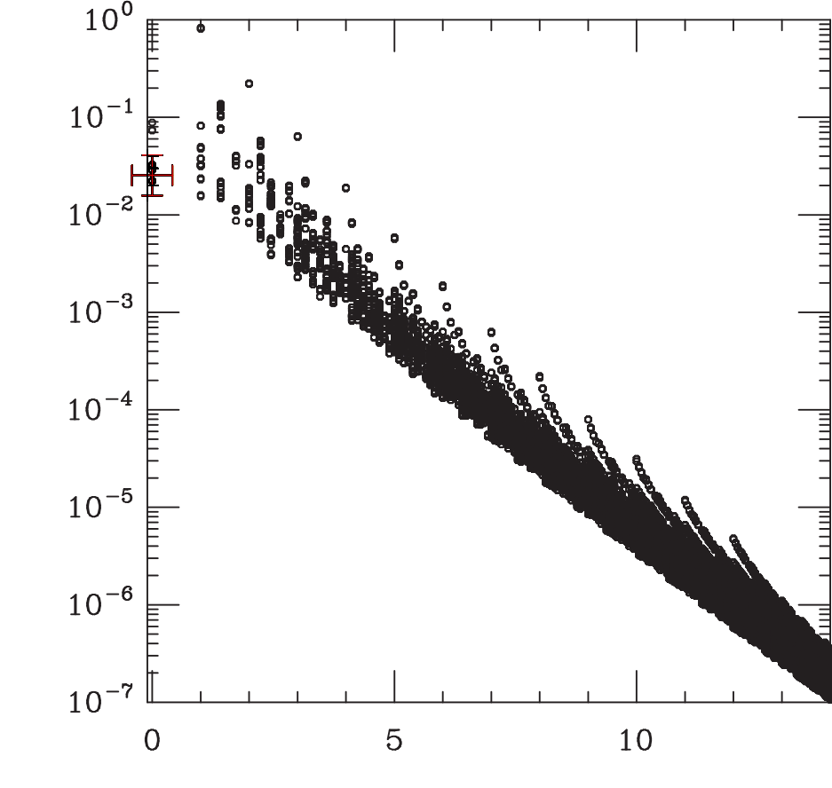
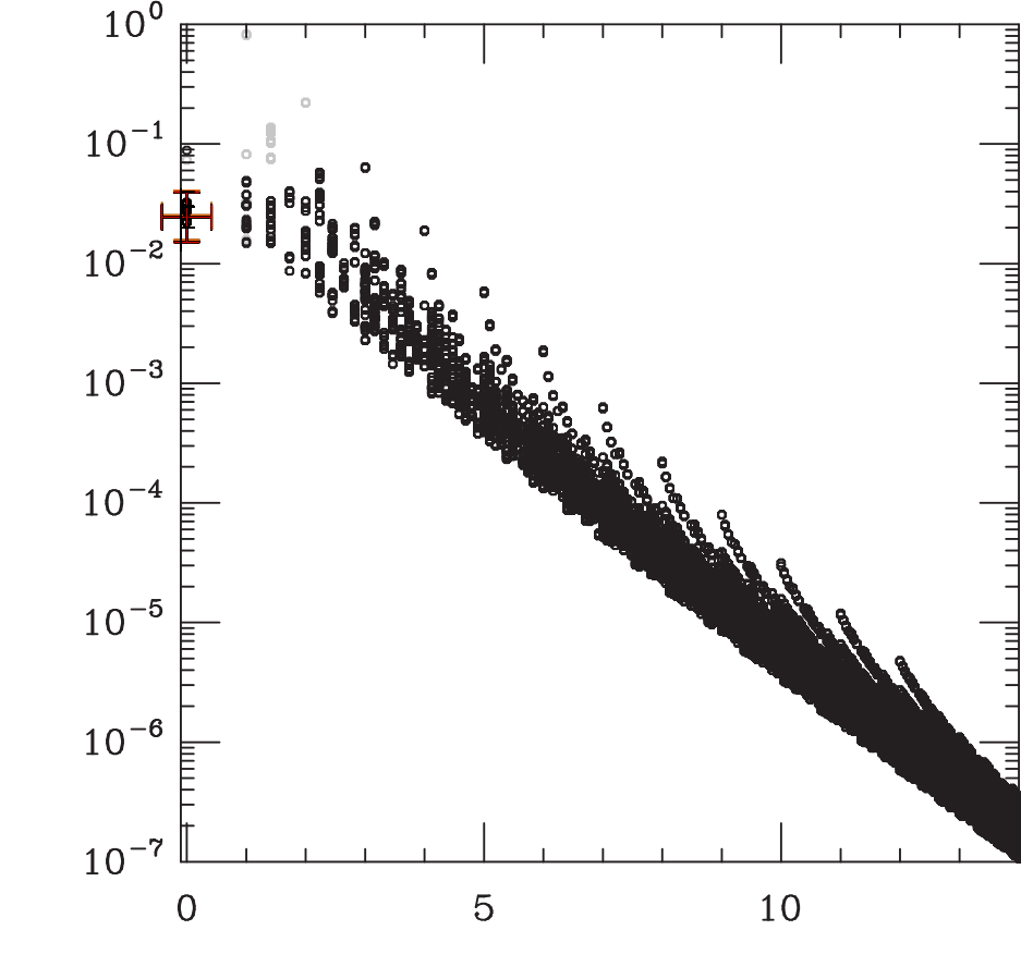
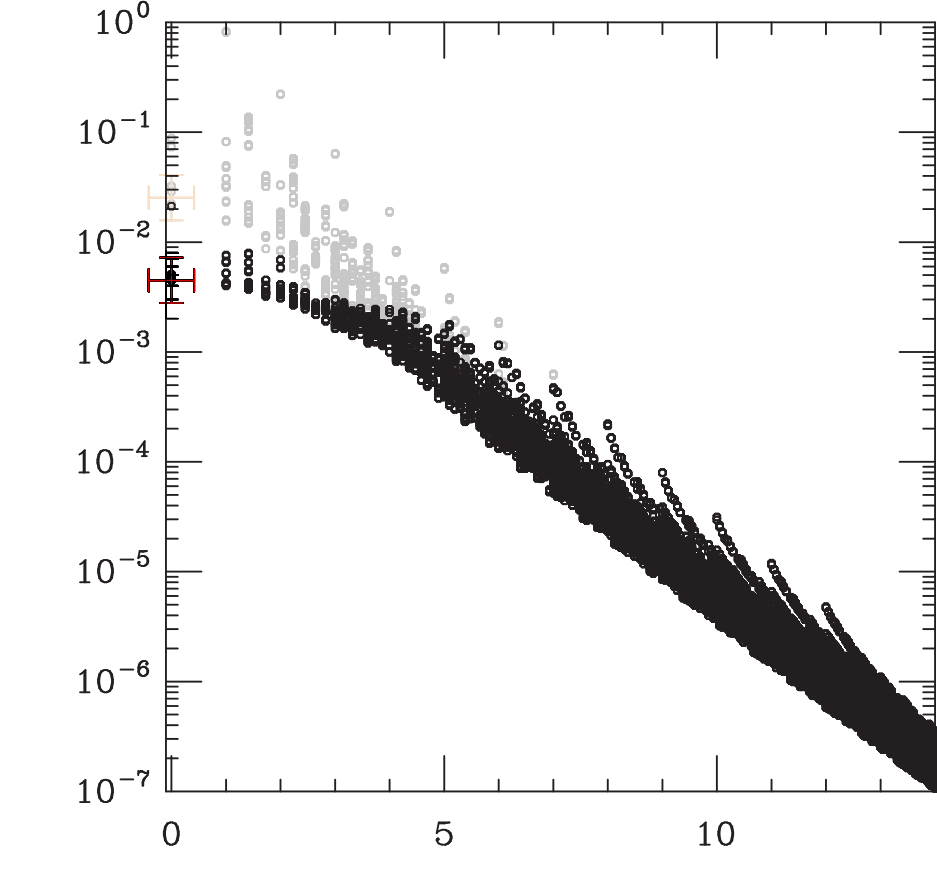
Figure 2: Map of the size of a large number of representative off-diagonal elements of ${{\partial M}\over{\partial\eta}}M^{-1}$ as a function of their Euclidean distance from the diagonal, ignoring spin and color, with different levels of hopping parameter improvement. Elements which share a separation vector (and will thus contribute to any particular dilution or HPE improvement scheme in the same way) are averaged together. The diagonal element, our signal, is shown as a cross potent at $x=0$. The left panel shows the unimproved operator. The middle panel shows the effect of second-order HPE, with the original operator shown in grey for comparison. The right panel shows the effect of seventh-order HPE, as applied in our calculation. Note that the plots say nothing about the number of elements at any given distance, which scales as $x^{4}$ and leads to larger contributions at larger distances.

4 Results

We have generated stochastic estimates of ${{\partial w}\over{\partial\eta}}$ and ${{\partial^{2}w}\over{\partial\eta}^{2}}$ on each configuration in the ensemble. The estimates of ${{\partial w}\over{\partial\eta}}$ use a minimum of 3000 $Z(4)$ noises, and the estimates of ${{\partial^{2}w}\over{\partial\eta}^{2}}$ use 1000; on some configurations (in particular, the first hundred) we have used more. The HPE improvement has been carried out to $7^{\mathrm{t}h}$ order. Unfortunately, the result is still very noisy. We performed a constant fit to the weight factors and their stochastic errors to determine whether any gauge variation (signal) is resolvable through the stochastic noise. For ${{\partial w}\over{\partial\eta}}$ some signal is apparent as the $\chi^{2}$/d.o.f. is somewhat greater than one, although the noise is still very high; for ${{\partial^{2}w}\over{\partial\eta}^{2}}$ nothing but noise is visible. These estimates are shown in Fig. 3.

Figure 3: Stochastic estimates of ${{\partial w}\over{\partial\eta}}$ (left) and ${{\partial^{2}w}\over{\partial\eta}^{2}}$ (right) on the 300 configurations. Stochastic error bars are shown. The different behavior in the first third of the ensemble for ${{\partial^{2}w}\over{\partial\eta}^{2}}$ is due to extra stochastic estimates in that portion. The $\chi^{2}$/d.o.f. of a constant fit, as a measure of the amount of signal resolvable through the noise, is shown for each term.

To finish the calculation, we must choose a particular $\eta$ at which to evaluate the weight factors. We originally computed valence correlators at $\eta=0.0051$; however, when the weight factor power series is evaluated at this $\eta$, the $w_{i}$’s are all negative. This is because ${{\partial^{2}w}\over{\partial\eta}^{2}}$ has a large negative average, as shown in Fig. 3. This represents a constant shift in the action independent of the gauge configuration (which should have no physical effect). While it is possible to construct an alternate expansion for the weight factor that causes this to cancel, it is still an indication that we are not in the regime where $\Delta S\ll 1$. They are much better behaved at $\eta=10^{-4}$; see Fig. 4. We thus “rescale” the valence correlators to $\eta=10^{-4}$ by fitting to $G(T,\eta)=G(T,0)+A(T)\eta+B(T)\eta^{2}$; the rescaled correlators, as well as the valence-only polarizability fits, are essentially identical for newly-run correlators at $\eta=10^{-4}$ and rescaled ones starting from $\eta=0.0051$[12].

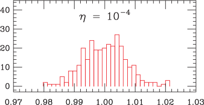
Figure 4: Distributions of the resulting weight factors when the expansion for $w(\eta)$ is evaluated at $\eta=0.0051$ (left panel) and $\eta=10^{-4}$ (right panel).

We have performed the reweighting order-by-order (turning on first the ${{\partial w}\over{\partial\eta}}$ term, then ${{\partial^{2}w}\over{\partial\eta}^{2}}$) to see the effects, which are shown in Table  1. While including the first-order reweighting inflates the error bar somewhat, the full second-order reweighting greatly increases the statistical error.

Reweighting order	$a\Delta E_{n}$
$0^{\rm{th}}$ order (unreweighted)	6.01(88) $\times 10^{-7}$
$1^{\rm{st}}$ order	2.86(2.32) $\times 10^{-7}$
$2^{\rm{nd}}$ order (full calculation)	17.8(10.9) $\times 10^{-7}$

Table 1: Results for the change in the neutron energy when reweighting is turned on order by order.

5 Further improving the weight factors and future plans

The large increase in the statistical error on the full calculation is driven by the stochastic estimator fluctuations in the weight factors. One possibility is to simply increase the number of stochastic estimates. Another possibility is the use of dilution. It is somewhat redundant with the HPE procedure since both aim to reduce or eliminate the contribution of the large near-diagonal elements to the stochastic noise. Preliminary tests of very aggressive dilution suggest that it can greatly reduce the stochastic noise; for a given amount of GPU time the optimum strategy seems to be to use the strongest possible dilution scheme for which one estimate per configuration is affordable, rather than attempting to gain statistics by repeating a weaker dilution scheme.

6 Acknowledgements

This work is supported in part by the NSF CAREER grant PHY-1151648 and the U.S. Department of Energy grant DE-FG02-95ER-40907.

References

- [1] H.R. Fiebig, W. Wilcox, and R.M. Woloshyn. A Study of Hadron Electric Polarizability in Quenched Lattice QCD. Nucl.Phys., B324:47, 1989.
- [2] Joseph C. Christensen, Walter Wilcox, Frank X. Lee, and Le-ming Zhou. Electric polarizability of neutral hadrons from lattice QCD. Phys.Rev., D72:034503, 2005.
- [3] Michael Engelhardt. Progress Toward the Chiral Regime in Lattice QCD Calculations of the Neutron Electric Polarizability. PoS, LAT2009:128, 2009.
- [4] W. Detmold, B.C. Tiburzi, and A. Walker-Loud. Extracting Nucleon Magnetic Moments and Electric Polarizabilities from Lattice QCD in Background Electric Fields. Phys.Rev., D81:054502, 2010.
- [5] Andrei Alexandru and Frank X. Lee. The Background field method on the lattice. PoS, LATTICE2008:145, 2008.
- [6] H. Ohki, S. Aoki, H. Fukaya, S. Hashimoto, T. Kaneko, et al. Nucleon sigma term and strange quark content in 2+1-flavor QCD with dynamical overlap fermions. PoS, LAT2009:124, 2009.
- [7] Walter Freeman, Andrei Alexandru, Frank Lee, and Michael Lujan. Sea Contributions to Hadron Electric Polarizabilities through Reweighting. PoS, LATTICE2012:015, 2012.
- [8] Anna Hasenfratz, Roland Hoffmann, and Stefan Schaefer. Hypercubic smeared links for dynamical fermions. JHEP, 0705:029, 2007.
- [9] R. Sommer. A New way to set the energy scale in lattice gauge theories and its applications to the static force and alpha-s in SU(2) Yang-Mills theory. Nucl.Phys., B411:839–854, 1994.
- [10] Anna Hasenfratz, Roland Hoffmann, and Stefan Schaefer. Reweighting towards the chiral limit. Phys.Rev., D78:014515, 2008.
- [11] C. Thron, S.J. Dong, K.F. Liu, and H.P. Ying. Pade - Z(2) estimator of determinants. Phys.Rev., D57:1642–1653, 1998.
- [12] M. Lujan, A. Alexandru, W. Freeman, and F.X. Lee. Valence calculation of the electric polarizability on nHYP-Clover ensembles. PoS, Lattice 2013:287, 2013.