The superluminous supernova PS1-11ap: bridging the gap between low and high redshift

Abstract

We present optical photometric and spectroscopic coverage of the superluminous supernova (SLSN) PS1-11ap, discovered with the Pan-STARRS1 Medium Deep Survey at $z=0.524$. This intrinsically blue transient rose slowly to reach a peak magnitude of $M_{u}=-21.4$ mag and bolometric luminosity of $8\times 10^{43}$ ergs^-1 before settling onto a relatively shallow gradient of decline. The observed decline is significantly slower than those of the superluminous type Ic SNe which have been the focus of much recent attention. Spectroscopic similarities with the lower redshift SN2007bi and a decline rate similar to ⁵⁶Co decay timescale initially indicated that this transient could be a candidate for a pair instability supernova (PISN) explosion. Overall the transient appears quite similar to SN2007bi and the lower redshift object PTF12dam. The extensive data set, from 30 days before peak to 230 days after allows a detailed and quantitative comparison with published models of PISN explosions. We find that the PS1-11ap data do not match these model explosion parameters well, supporting the recent claim that these SNe are not pair instability explosions. We show that PS1-11ap has many features in common with the faster declining superluminous Ic supernovae, and the lightcurve evolution can also be quantitatively explained by the magnetar spin down model. At a redshift of $z=0.524$ the observer frame optical coverage provides comprehensive restframe UV data and allows us to compare it with the superluminous SNe recently found at high redshifts between $z=2-4$. While these high-z explosions are still plausible PISN candidates, they match the photometric evolution of PS1-11ap and hence could be counterparts to this lower redshift transient.

1 Introduction

Recent wide field surveys, such as the Palomar Transient Factory (PTF) (Law et al., 2009; Rau et al., 2009) and Pan-STARRS1 (PS1) (Kaiser et al., 2010) have uncovered that the schema for classifying the highly luminous and energetic endpoints of massive stars known as supernovae (SNe) may be more complicated than previously thought. Quimby et al. (2011) linked the peculiar SCP06F6 (Barbary it et al., 2009) with a number of PTF discoveries to suggest the emergence of a new class of superluminous supernovae (SLSNe) characterised by peak absolute magnitudes of $<-21$ mag with total radiated energies of $\sim 10^{51}$ erg and a preference for low luminosity hosts. A number of similar objects were discovered at higher redshifts with PS1 cementing the notion that new types of SNe were being discovered (Chomiuk et al., 2011; Berger et al., 2012; Chornock et al., 2013; Lunnan et al., 2013).

Gal-Yam (2012a) proposed a three tier classification scheme for these objects of SLSNe-I, SLSNe-II and SLSNe-R based on the observed photometric, spectroscopic and supposed physical properties. Inserra et al. (2013) have recently presented an extensive study of low redshift SLSNe with data before peak and late photometric coverage to beyond 200 days. As found by Pastorello et al. (2010) for SN2010gx, these SNe evolve to resemble type Ic SNe but on much slower timescales. Hence Inserra et al. (2013) have termed this class SLSN-Ic as they are superluminous and (in the standard classification definitions) of type Ic as they lack hydrogen and helium lines. These are the type called SLSNe-I by Gal-Yam (2012a) (and elsewhere in the literature) but we will use the term SLSN-Ic throughout this paper. Inserra et al. (2013) have proposed that the lightcurves for these SLSN-Ic can be quite well fit with the deposition of energy from a spinning down magnetic neutron star.

Of particular interest here is the so-called SLSNe-R class which derives its name from the slow decline in the post-peak light curve. This luminosity could possibly be powered by the radioactive decay of a large mass of ⁵⁶Ni created in the explosion decaying to ⁵⁶Co and ⁵⁶Fe, hence the ‘R’ in the name. One event that has previously been classified as such is SN2007bi (Gal-Yam et al., 2009; Young et al., 2010). This SLSN was proposed by Gal-Yam et al. (2009) to be the result of electron-positron pair production in the core of an initially very massive ($M_{initial}>140\mbox{M${}_{\odot}$}$) star which reduces supporting radiation pressure and leads to gravitational contraction with a rise in core temperature above $10^{9}$K. The carbon-oxygen core at this point must be more massive than $\sim 60\mbox{M${}_{\odot}$}$ and undergoes explosive oxygen burning which can create an unusually large mass of ⁵⁶Ni. This Pair Instability Supernova (PISN), and the subsequent decay of the ⁵⁶Ni would provide the energy required to create the observed luminosity and unbind the star completely, leaving no remnant (Rakavy & Shaviv, 1967; Barkat it et al., 1967; Bond et al., 1984; Heger & Woosley, 2002; Langer et al., 2007).

Another possible mechanism for producing the large amount of ⁵⁶Ni required is the evolution of a slightly less massive carbon-oxygen core ($M<45\mbox{M${}_{\odot}$}$) until the more usual iron core-collapse (CCSN) process (Umeda & Nomoto, 2008; Moriya et al., 2010). This alternate process can reproduce the light curve shape of these objects but Gal-Yam (2012b) argued that they should lead to stronger nebular emission lines of Fe than were detected in the late-time spectra of SN2007bi. Cooke et al. (2012) proposed the discovery of another two such PISN candidates, thought to be at redshifts of $z\sim 2$ and $z\sim 4$, and PTF has discovered another possible candidate, PTF10nmn (Yaron et al, in prep).

However, the massive progenitors required for such a sequence of events to take place require the low metallicity environments such as those found only in the very early universe (Schneider et al., 2002; Bromm & Lebb, 2003). Emission lines from the host spectra of SN2007bi indicate that it is only at $z=0.128$, and Young et al. (2010) estimated a metallicity of around 0.3Z_⊙. This is much higher than what was originally expected for PISN or massive CCSNe progenitors, as by definition a massive carbon-oxygen core must have low enough mass-loss rates that it does not shrink to the typical Wolf-Rayet (WR) stellar masses (around 5-25M_⊙ Crowther, 2007) through strong radiatively driven winds. There is an obvious problem for SN2007bi in that we lack a physical model for the progenitor to exist with a core mass of around 60M_⊙ at this metallicity, if the typical mass-loss rates of massive stars at 0.3Z_⊙ or LMC type metallicities hold (Crowther et al., 2002; Crowther, 2007; Mokiem et al., 2007). Stellar evolutionary models all end with carbon-oxygen cores of much lower mass (e.g. Heger & Woosley, 2002; Heger et al., 2003; Eldridge & Tout, 2004; Langer et al., 2007). Although Langer et al. (2007) can produce PISN at metallicities seen in the nearby Universe, these models all produce hydrogen rich events and WR progenitor model explosions require significantly lower metallicity, typically below $0.05$Z_⊙. If, however, very massive stars ($M_{initial}\sim 320\mbox{M${}_{\odot}$}$) exist, Yusof et al. (2013) show that a PISN can be produced at $0.3$Z_⊙. For metallicites such as in the Small Magellanic Cloud (SMC), Yusof et al. (2013) manage to synthesise PISNe from stars with $100<M_{initial}<190\mbox{M${}_{\odot}$}$, where the very large convective cores of the stars during their main sequence phase allows them to evolve homogeneously. To achieve this however, the mass loss rates of these models must be set so that the stars lose their H envelope but retain their He layer, predicting that the resulting SNe may be of Type Ib as supposed to the observed Ic-like properties seen in SN2007bi. Dessart et al. (2012a) show that the detection of the He lines for a Type Ib SN requires not only the presence of helium but also the excitation source of ⁵⁶Ni to be well mixed. Hence a Type Ic PISN from the Yusof et al. (2013) models is plausible.

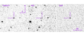
Figure 1: PS1 target, reference and difference images of PS1-11ap. The images are $i_{\rm P1}$-band.

Another very luminous supernovae, PTF12dam, has recently been discovered at the similar redshift of $z=0.107$. PTF12dam (Nicholl et al., 2013) shares similar photometric and spectroscopic properties to SN2007bi but a substantial dataset has allowed for more extensive modelling that points away from the PISN or ⁵⁶Ni-driven explanation. One possible alternative is that the energy injection required to explain the luminosity comes from the spin-down of a fast rotating neutron star or magnetar, which boosts the normal SN luminosity generating mechanisms. Inserra et al. (2013) have proposed that this mechanism could explain the faster declining SLSN-Ic in their low redshift sample, based on the recent theoretical treatment of Kasen and Bildsten (2010) and Woosley (2010). The idea of neutron star remnants powering the subsequent SN evolution dates back to Ostriker & Gunn (1971) and the energy input of highly magnetic neutron stars has been proposed to influence gamma-ray burst production (Usov, 1992; Wheeler et al., 2000). The production of hyper-energetic SNe due to the extraction of energy from a spinning down magnetar was suggested by Thompson et al. (2004), providing means for producing SNe with total radiated energies greater than $10^{51}$ ergs. In this paper we apply similar analysis to the SLSN PS1-11ap as done in Inserra et al. (2013) and Nicholl et al. (2013). We add fuel to the argument that if PISNe do exist, observational evidence for them has not yet been found.

2 Photometry

2.1 Pan-STARRS1

The PS1 system is a high-etendue wide-field imaging system, designed for dedicated survey observations. The system is installed on the peak of Haleakala on the island of Maui in the Hawaiian island chain. The telescope has a 1.8-m diameter primary mirror and the gigapixel camera (GPC1) located at the $f/4.4$ cassegrain focus consists of of sixty 4800$\times$4800 pixel detectors (pixel scale 0.258”) giving a field of view of 3.3^∘ diameter. Routine observations are conducted remotely, from the Waiakoa Laboratory in Pukalani. A more complete description of the PS1 system, both hardware and software, is provided by Kaiser et al. (2010). The survey philosophy and execution strategy are described in Chambers et al. (in prep)

The PS1 observations are obtained through a set of five broadband filters, which are designated as $g_{\rm P1}$, $r_{\rm P1}$, $i_{\rm P1}$, $z_{\rm P1}$, and $y_{\rm P1}$. Although the filter system for PS1 has much in common with that used in previous surveys, such as the Sloan Digital Sky Survey (SDSS) (Abazajian et al., 2009), there are important differences. The $g_{\rm P1}$ filter extends 20 nm redward of $g_{SDSS}$, paying the price of 5577Å sky emission for greater sensitivity and lower systematics for photometric redshifts, and the $z_{\rm P1}$ filter is cut off at 930 nm, giving it a different response than the detector response which defined $z_{SDSS}$. SDSS has no corresponding $y_{\rm P1}$ filter. Further information on the passband shapes is described in Stubbs et al. (2010). The PS1 photometric system and its response is covered in detail in Tonry et al. (2012a). Photometry is in the “natural” PS1 system, $m=-2.5\log(flux)+m^{\prime}$, with a single zeropoint adjustment $m^{\prime}$ made in each band to conform to the AB magnitude scale.

This paper uses images and photometry from the PS1 Medium-Deep Field survey (MDS), the strategy of which are described in Tonry et al. (2012b). Observations of between 3-5 medium deep (MD) fields are taken each night and the filters are cycled through in the following pattern : $g_{\rm P1}$ and $r_{\rm P1}$ in the same night (dark time), followed by $i_{\rm P1}$ and $z_{\rm P1}$ on the subsequent second and third nights respectively. Around full moon only $y_{\rm P1}$ data are taken. Any one epoch consists of 8 dithered exposures of either $8\times 113$s for $g_{\rm P1}$ and $r_{\rm P1}$ or $8\times 240$s for the other three, giving nightly stacked images of 904s and 1632s duration.

Images obtained by the PS1 system are processed through the Image Processing Pipeline (IPP) (Magnier, 2006), on a computer cluster at the Maui High Performance Computer Center (MHPCC). The pipeline runs the images through a succession of stages including device “de-trending”, a flux-conserving warping to a sky-based image plane, masking and artifact location. De-trending involves bias and dark correction and flatfielding using white light flatfield images from a dome screen, in combination with an illumination correction obtained by rastering sources across the field of view. After determining an initial astrometric solution the flat-fielded images were then warped onto the tangent plane of the sky using a flux conserving algorithm. The plate scale for the warped images was originally set at 0.200 arcsec/pixel, but has since been changed to 0.25 arcsec/pixel in what is known internally as the V3 tesselation for the MD fields. Bad pixel masks are applied to the individual images and carried through the stacking stage to give the “nightly stacks” of 904s and 1632s total duration. Two independent difference imaging pipelines run on a daily basis on the MD fields.

The PS1 project has developed the Transient Science Server (TSS) which takes the nightly stacks created by the IPP in MHPCC, creates difference images with respect to high quality reference images, and then carries out point source function (PSF) fitting photometry on the difference images to produce catalogues of variables and transient candidates (initially described in Gezari et al., 2012). All these individual detections are ingested into a MySQL database residing at Queen’s University Belfast (QUB) after an initial rejection algorithm based on the detection of saturated, masked or suspected defective pixels within the PSF area. Sources are assimilated into transient candidates if they have more than 3 quality detections within the last 7 observations of the field, including detections in more than one filter, and an RMS scatter in the positions of $\leq 0\aas@@fstack{\prime\prime}5$. Each quality detection must be of more than $5\sigma$ significance (defined as instrumental magnitude error $<0.2^{m}$) and have a Gaussian morphology ($XY_{moments}<1.2$). Transient candidates which pass this automated filtering system are promoted for human screening, which currently runs at around 10% efficiency (i.e. 10% of the transients promoted automatically are judged to be real after human screening). These real transient candidates are crossmatched with all available catalogues of astronomical sources in the MDS fields. We use our own MDS catalogue and also extensive external catalogues (e.g. SDSS, GSC, 2MASS, APM, Veron AGN, X-ray catalogues) in order to have a first pass classification of supernova, variable star, active galactic nuclei or nuclear transient.

In parallel, an independent set of difference images are produced at the Centre for Astrophysics (Harvard) on the Odyssey cluster from these IPP nightly stacked images using the $photpipe$ (Rest et al., 2005) software. A custom built reference stack is produced and each IPP nightly stack uses this to produce an independent difference image. This process is described in Gezari et al. (2010); Chomiuk et al. (2011); Berger et al. (2012); Gezari et al. (2012); Chornock et al. (2013); Lunnan et al. (2013) and potential transients are visually inspected for promotion to the status of transient alerts. We cross match between the TSS and the $photpipe$ transient streams and agreement on the detection and photometry is now excellent, particularly after the application of uniform photometric calibration based on the “ubercal” process (Schlafly et al., 2012; Magnier et al., 2013).

2.2 Photometric observations

Figure 2: Optical photometry for PS1-11ap. The dashed lines show the host galaxy magnitudes from the pre-explosion PS1 images also with linear offsets as noted in the figure key and the arrows indicate limiting magnitudes when a detection of the transient could not be obtained above a 3$\sigma$ limit.

PS1-11ap was discovered as a bright transient object in the PS1 Medium Deep Field 05 (MD05) on the 31st December 2010 at a J2000 location of RA = 10^h48^m27^s.73, Dec = 57^∘09^′09^′′.2. As a high significance transient, it was discovered simultaneously in both the TSS and $photpipe$ parallel searches. Fig. 1 shows that a faint host is present in the PS1 reference image but that the post explosion image shows the transient as significantly brighter than its host galaxy. The object was initially observable from Hawaii until the 29th June 2011, at which point it disappeared behind the sun, and griz$y_{\rm P1}$ exposures were taken throughout this entire period (referred to here as the first season). Accompanying this was griz photometry (SDSS filters) taken with the 2-m Liverpool Telescope + RATCam (LT) on La Palma which was useful for completeness when PS1 was experiencing downtime from bad weather. This additional photometry was particularly useful during the period between the Modified Julian Dates (MJD) of 55610 and 55640 when the supernova was at its peak brightness as PS1 was unavailable at this time. A MJD $=55613$ is used as the peak epoch of the SN, deduced by fitting a low order polynomial to the photometric $r_{\rm P1}$-band data. PS1 started observing MD05 again on MJD $=55904$ (9th December 2011) and the transient was still visible in the $r_{\rm P1}$, $i_{\rm P1}$ and $z_{\rm P1}$-bands (referred to here as the second season). A number of photometric points could be retrieved at this date by manually subtracting pre-explosion reference images from each epoch to remove any flux contamination from the faint host galaxy and by co-adding multiple exposures together, the methodology of which is subsequently explained.

Photometry during the first season of PS1 data was carried out using difference images and measurement routines within the $photpipe$ pipeline (Rest et al., 2005) using stacked pre-explosion PS1 exposures as a reference image. Details of these photometric measurements are presented in Chomiuk et al. (2011); Berger et al. (2012); Gezari et al. (2012) and Nicholl et al. (2013) and will be given in more detail in Rest et al. (2013, sub.) and Scolnic et al. (2013, sub.). The LT data were processed through the LT detrending system which debiases and flat-fields images. We built our own fringe frames to subtract from the i and z-band exposures. Photometric measurements of PS1-11ap were completed by performing PSF-fitting photometry within iraf using the custom built snoopy package. No image subtraction was carried out on the LT data as the transient was significantly brighter than its host. The effects of fringing were particularly apparent in the z-band exposures and were difficult to completely remove at times hence the increased scatter in the LT z-band photometry. Zero points for each image were calculated using magnitudes from a number of bright SDSS stars. Filter transformations, as detailed in Tonry et al. (2012a), were applied to each filter to correct all the SDSS griz magnitudes to PS1 gri$z_{\rm P1}$ magnitudes.

Difference imaging of the second season data was carried out by creating custom reference images from pre-explosion PS1 exposures obtained during the period between MJD 55160 and 55350. Approximately 8 nightly stacks were manually picked as high quality images in each filter and were median combined using the imcombine task in iraf for each filter. These reference images could then be subtracted from the second season PS1 observations using hotpants, an implementation of the Alard algorithm (Alard, 2000). This is the same algorithm as used in $photpipe$ for earlier epochs, hence the methods are consistent. To improve the signal in the images the data were binned into 30 day periods and PSF-fitting photometry was again performed using snoopy. The detections show a slowly fading tail phase during this late monitoring phase and the co-added frames considerably help with detections. During the 3 year lifetime of PS1 no previous outbursts for PS1-11ap have been detected before the first detection in December 2010. The griz$y_{\rm P1}$ light curves can be seen in Fig. 2 where the dotted lines represent the host magnitudes, obtained by performing aperture photometry on the pre-explosion, combined images (see Sect. 3.3).

Table 1: Central rest wavelengths (Å) of optical passbands for each of the SLSNe used in this paper. The numbers in italic show the filters used for comparisons. The redshift of each object is also given in the top row.

Filter		PS1-11ap	PTF12dam	SN2007bi	SN2011ke	SN2010gx	SN2213-1745
	-	0.524	0.107	0.127	0.143	0.230	2.05
u	3540	-	3196	-	3097	2878	-
B	4445	-	-	3945	3890	-	-
g	4860	3193	4396	-	4257	3878	$\sim 1600$
V	5505	-	-	4885	4817	-	-
r	6230	4091	5632	5528	5455	5065	$\sim 2050$
i	7525	4939	6799	6673	6585	6199	$\sim$2530
z	8660	5680	7820	-	7573	7426	-
y	9720	6382	8786	-	-	-	-

$\begin{array}[]{cc}\includegraphics[angle={270},scale={0.425}]{figs/11ap_ablccomp.eps}\\ \includegraphics[angle={270},scale={0.425}]{figs/11ap_pisncomp.eps}\\ \end{array}$

Figure 3: (TOP PANEL) An absolute magnitude comparison of $z_{\rm P1}$-band PS1-11ap data with r-band PTF12dam, SN2007bi  SN2011ke and i-band SN2010gx data. See text for appropriate references. All of these are absolute AB magnitudes calculated without a detailed $K-$correction using Eq. 1. (BOTTOM PANEL) A comparison of $g_{\rm P1}$-band PS1-11ap with i-band SN2213-1745 and g and u-band PTF12dam. Also included here are two PISNe models similar to that used by Cooke et al. (2012) to fit the SN2213-1745 data. As in the Cooke et al. (2012) paper, the models have been offset to match the luminosity of the data.

The two arrows during the season 2 data points indicate epochs at which no transient could be detected at the position of PS1-11ap at greater than three times the level of the background noise. Of note regarding the colour evolution of the light curves is that the $g_{\rm P1}$ and $r_{\rm P1}$-band light curves decline much quicker than the redder filters. This is to be expected as heavier elements in the spectra for PS1-11ap at the derived rest wavelength covering the $g_{\rm P1}$-band filter may cause a line blanketing effect. This is discussed in Section 3 along with a more in-depth look at the temperature evolution of PS1-11ap.

K-correction values were calculated using spectra from the 22nd February, 11th March, 22nd April and 22nd June. As these observations were reasonably frequent no intermediate measures were required to fill in lengthly gaps between epochs when a spectrum was not available. All the photometric values deduced for PS1-11ap could then be corrected at all epochs using the nearest possible K-correction value. At the redshift of PS1-11ap the conversion filters correspond to the following rest frame filters; $g_{\rm P1}$$\to UV_{uvw1}$, $r_{\rm P1}$$\to u_{SDSS}$, $i_{\rm P1}$$\to g_{SDSS}$, $z_{\rm P1}$$\to r_{SDSS}$, $y_{\rm P1}$$\to i_{SDSS}$. Details of all the photometry and K-correction data for PS1-11ap can be found in Appendix A.

Figure 4: The complete spectral series for PS1-11ap in the galaxy restframe. Telluric features that have not been removed are marked with a ‘$\oplus$’.

Table 2: Information on all of the spectra obtained for PS1-11ap.

Date	MJD	Phase (rest)	Telescope	Grating	Wavelength range (Å)	Resolution (Å)	P.I.
24/01/2011	55585	-20 days	GN + GMOS	R400	$5440-9650$	5	J. Tonry
06/02/2011	55598	-11 days	NOT + ALFOSC	Gm14	$3500-8800$	13	R. Kotak
22/02/2011	55614	-1 days	WHT + ISIS	R300B; R158R	$3160-10,500$	6	S. Smartt
11/03/2011	55631	+10 days	GN + GMOS	R150	$4120-10,500$	12	A. Pastorello
31/03/2011	55651	+24 days	APO + DIS	B400; R300	$3700-9000$	7	M. Huber
06/04/2011	55657	+28 days	MMT + HECTOSPEC	270	$3700-9150$	5	E. Berger
22/04/2011	55673	+38 days	GN + GMOS	R150	$4500-10,500$	12	A. Pastorello
08/06/2011	55720	+69 days	MMT + HECTOSPEC	270	$3700-9150$	5	E. Berger
22/06/2011	55734	+78 days	GN + GMOS	R150	$4000-10,500$	12	D. A. Howell
27/12/2011	55922	+201 days	GN + GMOS	R400	$5000-9320$	5	S. Smartt

2.3 Comparisons with SLSNe

A photometric comparison of PS1-11ap with the SLSNe PTF12dam, SN2007bi, SN2011ke and SN2010gx (Nicholl et al., 2013; Gal-Yam et al., 2009; Young et al., 2010; Inserra et al., 2013; Pastorello et al., 2010; Quimby et al., 2011) is shown in Fig. 3. To compare the respective absolute AB magnitude of each supernova we used the following:

$$M=m-5log(\frac{d_{L}}{10(pc)})+2.5log(1+z)$$ (1)

(Hogg et al., 2002), where m is the apparent AB magnitude. This corrects the measured magnitudes for cosmological expansion but is not a proper K-correction. To make the comparison between different objects valid, appropriate filters were chosen so that the central rest wavelengths were as similar as possible (details of this are shown in Table 1). Note that although full K-correction data for PS1-11ap is given in this paper (see Appendix A) and for PTF12dam in Nicholl et al. (2013), all the SLSNe data used here are treated with the same pseudo-correction given in Eq. 1 to ensure a reasonably consistent comparison. A standard cosmology with $H_{0}=72$ kms^-1, $\Omega_{M}=0.27$ and $\Omega_{\lambda}=0.73$ is used throughout.

Two distinct groups of objects can clearly be seen in this plot; those transients with steeply-declining light curves post peak and those with long-lived light curves, falling by no more than $\sim$ 2 mag in 100 days. PS1-11ap seems to belong to this latter group. The only SN to previously fall definitively into this class was SN2007bi. Gal-Yam et al. (2009) suggested that the shallow gradient was powered by the radioactive decay of ⁵⁶Ni $\to$ ⁵⁶Co $\to$ ⁵⁶Fe synthesised as a result of a PISN. The recent discovery of PTF12dam (Nicholl et al., 2013) and the data for PS1-11ap presented in this paper allow us to shed new light on this class of objects.

Fig. 3 also shows a comparison of a PS1-11ap $g_{\rm P1}$-band light curve with an i-band light curve of the high redshift ($z=2.046$) SN2213-1745 (Cooke et al., 2012), g and u-band light curves of the low redshift ($z=0.107$) PTF12dam (Nicholl et al., 2013) and PISNe model fits for a 100M_⊙ and a 130M_⊙ bare helium core (Kasen et al., 2011). The PISNe model light curves were calculated by applying a synthetic SDSS u-band filter ($\lambda_{c}=3550$Å) to the model PISN spectra from Kasen et al. (2011) at all epochs using the synphot function within iraf. This gave model observed light curves in magnitudes which could be offset to the same peak absolute magnitudes as the SLSN data by subtracting an arbitrary constant from each model. No scaling for time dilation (as the observed data were already corrected to rest frame) or colour corrections were applied. The data for PS1-11ap, PTF12dam and SN2213-1745 all illustrate that their light curves may be similar. It is possible that SN2213-1745 is akin to these lower redshift SLSN counterparts. The differences in the peak magnitudes could be due to the nature of the pseudo-correction applied or evidence of intrinsic variation within this group of SLSNe. However this conclusion relies on the assumption that the missing epochs for SN2213-1745 would follow the same trend as PS1-11ap and PTF12dam. We acknowledge that this is somewhat speculative. Given the high redshift of the Cooke et al. (2012) PISN candidate, the central rest wavelengths compared are also quite different. The Cooke et al. (2012) data probe further into the UV than the data in this paper or in Nicholl et al. (2013) which must be taken into account regarding any statements on the physical nature of SN2212-1745. In summary, the rise times of SN2213-1745, PS1-11ap and PTF12dam appear similar and the peak magnitudes and decay times are also not dissimilar. It is possible, but not confirmed, that all three objects belong in the same class.

This highlights the uniqueness of the PS1-11ap dataset and the importance of comparing data with similar central rest wavelengths, hence the inclusion of the u-band PTF12dam points around peak. The observed light curves of PS1-11ap (Fig. 2) show a marked difference in the evolution of the bluer bands. The observed $g_{\rm P1}$-band light curve, corresponding to an ultraviolet rest wavelength (see Table 1 for the central rest wavelengths of all the SLSNe mentioned and their corresponding observed filters), declines much more quickly than the red filters which fall into the NUV and optical regions after redshift corrections. The comparison seen in Fig. 3 shows that PS1-11ap and PTF12dam have a similar light curve evolution in the $\sim$NUV/optical filters but the higher redshift of PS1-11ap allows us a look into the UV that bridges the gap between the low redshift objects of this SLSNe class (2007bi and PTF12dam), and the high redshift examples in Cooke et al. (2012). Unfortunately u-band data for PTF12dam was only available for a short period around the peak epoch. PTF12dam has the most comprehensively observed rise time data of an object of this supposed class but Nicholl et al. (2013) also find that PISN models are poor fits to the rise time data for PTF12dam with PISN models.

3 Spectra

3.1 Dataset

$\begin{array}[]{cc}\includegraphics[angle={270},scale={0.35}]{figs/11ap_hostspec.eps}&\includegraphics[angle={270},scale={0.35}]{figs/11ap_mgIIsn.eps}\\ \end{array}$

Figure 5: The left-hand panel shows the narrow emission lines in a late time GMOS-N spectrum for PS1-11ap used to infer the redshift of the host galaxy as $z=0.524$. Another GMOS-N spectrum for a late epoch of PTF12dam is overplotted to highlight the similarities between the objects even at this late stage. The right-hand plot is a detail of the WHT PS1-11ap spectrum showing the rest wavelength of the two absorption features thought to be the Mg ii $\lambda\lambda$2796, 2803 doublet used to confirm the redshift value of the SN. The red line overplotted here shows the three Gaussian fits used (any values listed on this plot are in Å).

Optical spectra of PS1-11ap were obtained with the Gemini North (GN) telescope with GMOS-N, Nordic Optical Telescope (NOT) with the ALFOSC spectrograph and the William Herschel Telescope (WHT) with ISIS. Additional data were also provided from the Multiple Mirror Telescope (MMT) and the Apache Point Observatory (APO). In total, 11 epochs were obtained including a late-time GMOS-N spectrum obtained on 27 December 2011 (during the second season) in an attempt to gather data on either late-time spectra of the SN and/or the host galaxy. During the PS1-11ap season 1 at least one spectrum was obtained for each month that the SN was visible. Details of the spectral series are given in Table 2.

The WHT and NOT spectra were extracted using the iraf apall task after the usual de-bias and flat-fielding procedures. The GN spectra were extracted using the custom built gemini iraf package. All epochs were wavelength calibrated using spectra of CuAr lamps taken on the same respective epoch as the science frames and flux calibrated using observations of spectroscopic standard stars taken on epochs as close to the science frames as possible. Both the PS1-11ap GMOS-N spectra obtained on the 11th March and on the 22nd April were calibrated using a Feige34 spectrum taken on the 22nd April. The spectrum obtained on the 22nd June was calibrated using an observation of Feige34 from the same night and the spectrum from the 27th December was calibrated using a spectrum of Feige34 obtained on the 24th December. All the spectra for PS1-11ap can be seen in Fig. 4.

A redshift value of $z=0.524$ was initally derived for PS1-11ap from our first GMOS-N spectrum (taken in January 2011) from the narrow emission lines from the SN host galaxy. These are seen throughout the spectral series, most apparently in the late time GMOS-N spectrum as seen in Fig. 5. The use of the R400 grating for this early exposure however meant that a restframe wavelength range of just over 2500$\AA$ was obtained. Two spectra were obtained in February using the ALFOSC spectrograph and the ISIS spectrograph which both extend bluewards of $\sim 3500\AA$. This redshift means that the WHT restframe spectrum covers the Mg ii $\lambda\lambda$2796, 2803 doublet. This was initially used to determine the redshift of multiple SLSNe by Quimby et al. (2011) and Chomiuk et al. (2011) and subsequently Berger et al. (2012) illustrated its use in providing diagnostics of the ISM in the apparently unusual host galaxies of SLSNe. The redshift of $z=0.524$ was confirmed from simultaneous Gaussian fits to both components of the Mg ii $\lambda\lambda$2796, 2803 doublet, indicating that the absorption is very likely to be from the ISM of the host galaxy of PS1-11ap. By adopting the Mg ii centroids as rest frame the wider, bluer profile (assumed to be due to the supernova) could be fit with a simple Gaussian absorption profile (seen in Fig. 5). This provided an expansion velocity of $\sim 16,500$ kms^-1 which is similar to SLSNe which have previously been studied : velocities ranging from $10,000-20,000$ kms^-1 were found in Quimby et al. (2011); Chomiuk et al. (2011) and Inserra et al. (2013).

Three more GMOS-N spectra were taken in March, April and June this time utilising the R150 grating to increase the wavelength range of the exposures at the expense of some resolution. The APO and MMT data also offer some completeness around these epochs, although the low signal-to-noise limits their diagnostic usefulness. Finally, one more spectrum was obtained during the season 2 of PS1-11ap using the R400 grating to provide a resolution better matched to measuring the narrow galaxy emission lines ($\sim 300$ kms^-1). This was taken at a rest frame epoch of 201 days.

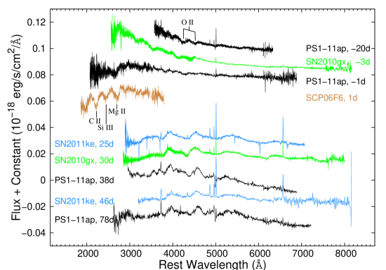
Figure 6: A spectral comparison of PS1-11ap with the SLSN Ic SN2010gx, SCP06F6 and SN2011ke.

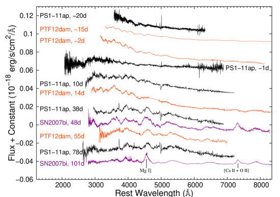
Figure 7: A spectral comparisons of PS1-11ap with PTF12dam and SN2007bi. Despite having spectral similarities with both SN2007bi-like objects and SLSN Ic we group PS1-11ap with the former due to its photometric evolution.

3.2 Spectral comparisons

Quimby et al. (2011) and Chomiuk et al. (2011) identified three broad absorption features in SLSNe-Ic at $\sim 2330\AA$ (C ii), $2543\AA$ (Si iii) and $2800\AA$ (Mg ii) as exemplified in the SCP06F6 spectrum (Quimby et al., 2011; Barbary it et al., 2009) in the comparison plot in Fig. 6. Here we see how the PS1-11ap data compares with data for the SLSNe-Ic SN2010gx, SCP06F6 and SN2011ke (Pastorello et al., 2010; Barbary it et al., 2009; Inserra et al., 2013). Between peak and 80 days, the PS1-11ap spectra are quite similar to these SLSNe-Ic. Two epochs of the PS1-11ap spectral series push bluewards of $\sim 2500\AA$ and broad Mg ii is seen in absorption in PS1-11ap (highlighted in the right hand plot in Fig. 5). Unfortunately neither the SN2007bi nor the PTF12dam spectra probe into the NUV. Another common feature that Quimby et al. (2011) identified with the SLSN-Ic class is a broad ‘W’-shaped feature at $\sim 4300\AA$ (O ii). This feature is also seen in the spectra of PS1-11ap and PTF12dam. The photometric evolution of PS1-11ap and objects of this class are very different, however, as previously discussed in Section 2.3.

We do not show a spectral comparison of PS1-11ap with objects from the SLSN-II class, such as SN2006gy (Smith et al. , 2007; Ofek et al., 2007), as none of the PS1-11ap spectra show any evidence of the broad H and He emission shown by SNe of this type.

The intermediate redshift of PS1-11ap makes a direct spectral comparison between it and SN2007bi and PTF12dam (both at redshifts of z$\sim 0.1$) difficult. Spectra for PS1-11ap are nevertheless compared with spectra for PTF12dam at all corresponding epochs and with spectra for SN2007bi at two later epochs (Nicholl et al., 2013; Young et al., 2010). Both the -20 day PS1-11ap spectrum and the -15 day PTF12dam spectrum (see Fig. 7) share a common blue colour with shallow, broad absorption features. The later spectra, especially around $\sim 50$ days, match very closely for all three objects. This similarity, combined with the photometric similarities in the slowly declining and very luminous light curves, provides convincing evidence that these objects are of the same physical class. Young et al. (2010) note that the spectra for SN2007bi are like that of a slowly evolving Type Ic SN but with an extremely extended photospheric phase that only begins its transition into the nebular phase at $350-400$ days post-discovery. Of interest is the appearance of nebular features, seen in the clear emission lines at $\sim 4500\AA$ (Mg i]) and $\sim 7320\AA$ (thought to be associated with the forbidden [Ca ii] $\lambda\lambda$7291, 7324 doublet and a forbidden emission feature of [O ii] at $7322\AA$) in both the 48 day and the 101 day SN2007bi spectra shown in Fig. 7, despite the clear presence of a retained continuum. When corrected for redshift, the wavelength coverage of the optical spectra for PS1-11ap only covers the Mg i] feature but it is also seen in the post peak epochs although not as strongly as in the case of SN2007bi.

A more detailed discussion on the nature of PS1-11ap is given in Section 4.

3.3 The Host Galaxy of PS1-11ap

Table 3: Main properties of the host galaxy of PS1-11ap. Foreground extinction was applied to determine of the absolute AB magnitudes at effective restframe noted.

PS1 Name	PSO J162.1155+57.1526
$g_{\rm P1}$(mag)	24.10 (0.32)
$r_{\rm P1}$(mag)	23.16 (0.17)
$i_{\rm P1}$(mag)	22.88 (0.15)
$z_{\rm P1}$(mag)	22.90 (0.24)
Internal extinction $A_{V}$ (mag)	$\sim 0$
$M_{\rm 316}$ (mag)	-17.79 (0.32)
$M_{\rm 405}$ (mag)	-18.72 (0.17)
$M_{\rm 493}$ (mag)	-19.00 (0.15)
$M_{\rm 568}$ (mag)	-18.97 (0.24)
Physical diameter (kpc)	3.6
Luminosity [O ii] (erg s-1)	$7.20\times 10^{40}$
SFR (M⊙ yr-1)	$0.47\pm 0.12$
Stellar Mass (M⊙)	$1.5^{+1.40}_{-0.65}\times 10^{9}$
sSFR (Gyr-1)	$0.31^{+0.24}_{-0.15}$

The host galaxy of PS1-11ap, PSO J162.1155+57.1526, was detected in $g_{\rm P1}$, $r_{\rm P1}$, $i_{\rm P1}$ and $z_{\rm P1}$-band PS1 images made from a co-addition of nightly images before the first discovery epoch of PS1-11ap. The host was not significantly detected in $y_{\rm P1}$-band stacks. The RA and Dec used for the position of the host galaxy were the same as that of PS1-11ap, given in Section 2.2, as the SN was coincident with the galaxy centroid.

The $i_{\rm P1}$-band image (total exposure time of 3840s) shows that there is a nearby fainter object at approximately 7 pixels from the centroid of the host galaxy of PS1-11ap. As the host was extended and not well described by a PSF, we chose to carry out aperture photometry with a 7 pixel aperture and applied an aperture correction using 8 isolated stars in the PS1 image (within 2 arcmin of the position of PS1-11ap).

We applied a correction for Milky Way extinction (Schlafly & Finkbeiner, 2011) and estimated the contribution of the nebular emission lines (discussed below) to the broad band photometry. This was required in order to determine the galaxy mass from stellar population model fitting to the observed galaxy colours. The correction was minimal and we found that the measured emission line strengths would only imply a change of 0.007 mag in $r_{\rm P1}$ and 0.01 mag in $i_{\rm P1}$. The absolute magnitudes are listed in Table 3 at the effective restframe wavelengths of the PS1 filters. A full K-correction was not calculated for these, they are simply estimated from Eq. 1. We used the MAGPHYS stellar population model code of da Cunha et al. (2008) with our redshift of $z=0.524$ with the goal of determining the stellar mass. The code returns a spectral energy distribution (SED) and best fit model, which is simply defined as the model with the lowest $\chi^{2}$ while allowing all the input parameters to vary. This lowest $\chi^{2}$ solution is plotted in Fig. 8 with the PS1-11ap host galaxy gri$z_{\rm P1}$ photometry where the x-axis error bars represent the PS1 filter bandpasses. The $\chi^{2}$ value is low ($\chi^{2}=0.011$) and not reflective of the range of acceptable fits for stellar mass. MAGPHYS gives a more realistic range of values for stellar mass by calculating the probability density function over a range of values and determining the median and the confidence interval corresponding to the 16th$-84$th percentile range. This is equivalent to the 1$\sigma$ range, if the distribution is roughly Gaussian (see da Cunha et al. 2008 for details). As recommended by da Cunha et al. (2008) we take the best estimate of stellar mass to be this median value, $1.5\times 10^{9}$M_⊙, and the 1$\sigma$ range to be $0.85-2.9\times 10^{9}$M_⊙. The best fit derived in Fig. 8 has a mass which is on the edge of the 1$\sigma$ range, $0.74\times 10^{9}$M_⊙, as this fit comes from allowing all parameters to vary and the range is from marginalising over stellar mass only. This illustrates that only the range should be considered as a reliable estimate, not a particular best fit.

Figure 8: Photometry of the host galaxy (red points) with the best-fit ($\chi^{2}$=0.011) model galaxy SED (black line) from MAGPHYS (da Cunha et al. 2008), with and without an attenuation by internal dust. This best fit model has a stellar mass of $7.4\times 10^{8}$M_⊙, but the more realistic range of masses is given in Table 3.

Table 4: Observed emission line strengths of the host of PS1-11ap taken by Gemini on 2011/12/27. The line strengths are as measured from the observed spectrum with no correction for redshift, extinction or distance yet. The last column is the equivalent width, in angstroms.

Line	Flux $\pm$ Error	EW
	(erg s-1 cm-2)	($\AA$)
$[$OII$]$ $\lambda$3727	$(6.90\pm 0.02)\times 10^{-17}$	39.82
H$\delta$ $\lambda$4102	$(5.47\pm 0.14)\times 10^{-18}$	3.16
H$\gamma$ $\lambda$4340	$(1.02\pm 0.05)\times 10^{-17}$	6.31
H$\beta$ $\lambda$4861	$(2.00\pm 0.03)\times 10^{-17}$	12.79
$[$OIII$]$ $\lambda$4959	$(2.75\pm 0.02)\times 10^{-17}$	15.20
$[$OIII$]$ $\lambda$5007	$(4.50\pm 0.02)\times 10^{-17}$	55.81

$\begin{array}[]{ccc}\includegraphics[angle={270},scale={0.3}]{figs/bb_-20_5.eps}&\includegraphics[angle={270},scale={0.3}]{figs/bb_-2_5.eps}\\ \includegraphics[angle={270},scale={0.3}]{figs/bb_12.eps}&\includegraphics[angle={270},scale={0.3}]{figs/bb_36.eps}\\ \includegraphics[angle={270},scale={0.3}]{figs/bb_74.eps}&\includegraphics[angle={270},scale={0.3}]{figs/phase_temp.eps}\\ \end{array}$

Figure 9: Blackbody fits to the PS1-11ap photometry with similar epoch spectra overplotted for consistency. The lower right figure shows how the fitted temperatures compare with the magnetar model fit from the lower right hand plot in Fig. 10, where the green shaded region covers the data of the four SLSN-Ic presented in Inserra et al (2013).

The final spectrum taken on 27 December 2011 with Gemini + GMOS still has clear signs of the broad lines from PS1-11ap (see Fig. 5). At this epoch of 201 days (restframe) the detected continuum is a combination of the host galaxy continuum ($r_{\rm P1}$$=23.16\pm 0.17$ from the pre-2011 data) and supernova flux ($r_{\rm P1}$$=23.68\pm 0.17$) measured in the reference subtracted images. Emission lines from the host galaxy are detected but at this redshift and without an infrared spectrum we are limited to the strong nebular lines visible between restframe wavelengths of $3700-5100$Å, as listed in Table 4. We fitted high order polynomials to the continuum and subtracted off this flux before measuring the emission line fluxes. Line fluxes were then measured using the QUB custom built $procspec$ environment within IDL and single Gaussian profiles were fit to each of the six identified features listed in Table 4. Although the [O ii] feature at 3727Å is a doublet blend, the two components were not resolved and a single Gaussian, broader than the other lines was employed. These are the observed line fluxes before any extinction or redshift corrections were applied. There is no detection of the electron temperature sensitive line [O iii] 4363Å, as used by Chen et al. (2013) and Lunnan et al. (2013) to determine abundances in the host galaxies of SN2010gx and PS1-10bzj. Hence we used the strong line $R_{23}$ method to estimate the oxygen abundance in the host.

To determine the intrinsic line emission strengths we first applied a correction for the Milky Way foreground extinction of $A(V)=0.02$ and $R_{V}=3.1$ (Schlafly & Finkbeiner, 2011). As we lacked H$\alpha$ in our optical spectra due to the redshift, we use the ratio of H$\gamma$/H$\beta$ to determine a value for internal extinction. The intrinsic line ratio assuming case B recombination for H$\gamma$/H$\beta=0.47$ and for H$\delta$/H$\beta=0.26$ (Osterbrock, 1989), which implies an internal dust extinction of $A(V)\sim 0$. The resultant spectrum was then shifted to rest wavelength for line measurements.

The reddening-corrected flux of the [O ii] $\lambda 3727$ line is $7.07\times 10^{-17}$ (erg s^-1 cm^-2) and so we determined the star formation rate (SFR) of the host to be $0.47\pm 0.12\,\mbox{M${}_{\odot}$}$ year^-1 from the relation of Kewley, Geller & Jansen (2004). Our restframe spectral coverage for PS1-11ap does not cover the wavelength of H$\alpha$ but as we know the intrinsic line ratio of H$\alpha$/H$\beta=2.86$ and have a measurement of H$\beta$, we can imply that the flux of H$\alpha=5.86\times 10^{-17}$ erg s^-1 cm^-2. From the calibration of Kennicutt (1998), SFR ($M_{\odot}$ year^-1)$=7.9\times 10^{-42}$ L(H$\alpha$) where the latter is in units of ergs s^-1, we calculate a SFR $\sim 0.47\pm 0.02\,\mbox{M${}_{\odot}$}$ year^-1, which shows a good agreement with the [O ii] result.

We determined the commonly used line ratio $R_{23}$ ([O iii] $\lambda\lambda 5007,4959$ + [O ii] $\lambda 3727$/H$\beta$) finding $\log(R_{23})=0.86$. This is close to the turnover region between lower and upper metallicity branches of the $R_{23}$ calibration plot and reduces our ability to constrain the metallicity particularly well. Using the McGaugh (1991) $R_{23}$ calibration, we determine $12+\log{\rm O/H}=8.5\pm 0.3$ dex for the upper branch, and $12+\log{\rm O/H}=8.1\pm 0.5$ dex for the lower. The large errors reflect the uncertainties from the line strength measurements. Typically there is also a systematic + 0.3 dex offset between the oxygen abundance determined with the $R_{23}$ ratio and the McGaugh (1991) calibration and abundances determined on an electron temperature scale (Bresolin, 2011). The $R_{23}$ calibration is uncertain and without a detection of an auroral line for electron temperature measurement (such as [O iii] $\lambda 4363$) we cannot determine the metallicity accurately. It is therefore possible, but not definitive, that the host is of low metallicity similar to that determined by Chen et al. (2013) and Lunnan et al. (2013) for the hosts of SN2010gx and PS1-10bzj respectively.

An additional probe of the host environment is ISM absorption of the Mg ii $\lambda\lambda$2796, 2803 doublet. This was a key diagnostic used by Quimby et al. (2011) and Chomiuk et al. (2011) to determine the redshifts of early SLSNe discoveries and Berger et al. (2012) illustrated the possible usage of these lines as diagnostics of the higher redshift Universe. Fig. 5 shows the Mg ii absorption detected in the WHT spectrum of PS1-11ap from the 22nd February, 2011. The rest frame equivalent widths of the two lines are $W_{r}(\lambda 2796)=0.8\AA$ and $W_{r}(\lambda 2803)=1.4\AA$ which are similar, within the errors, to those measured by Berger et al. (2012) for PS1-12bam.

3.4 Blackbody fits

Table 5: Temperatures from blackbody fitting of PS1-11ap.

Phase (rest)	$T_{bb}$
-20.5 days	16500 $\pm$ 3000 K
-2.5 days	12000 $\pm$ 2000 K
12 days	11500 $\pm$ 2000 K
36 days	8000 $\pm$ 1000 K
74 days	7000 $\pm$ 1000 K

Blackbody curves of various temperatures were fitted to the PS1-11ap photometry and spectra at 5 different epochs (listed in Table 5). The effective wavelength of each of the PS1 griz$y_{\rm P1}$ filters were taken from Tonry et al. (2012a) so that photometric data could be overplotted with an appropriate spectrum of similar phase. Model blackbody curves for various temperatures could then be manually fitted where the error range was derived simply by choosing the range of fits which still satisfied the data within 3 times the photometric errors. For example, a maximum and minimum temperature was selected for each epoch by trying to fit a range of blackbody curves to the photometric data until the fit passed through 3 times the error bars of less than 4 of the 5 effective wavelengths. The estimated temperature for that epoch was then given as the midpoint of the temperatures represented by these model curves with an error of the difference between them divided by 2. Effectively, the quoted errors for the blackbody fits are to approximately 3$\sigma$. It can be seen in Fig. 9 that the model curves fit the $r_{\rm P1}$, $i_{\rm P1}$, $z_{\rm P1}$ and $y_{\rm P1}$-band points well but that the $g_{\rm P1}$-band consistently falls short. This may be due to line blanketing from heavier elements at this wavelength range, supported by the broad absorption features seen in the spectra here.

A correction of $E(B-V)=0.006$ mag for Milky Way extinction in the direction of PS1-11ap from the NASA/IPAC IRSA dust maps (Schlafly & Finkbeiner, 2011) was applied to the photometry in each filter and each spectrum was corrected using the dered function in the iraf onedspec package. No correction was applied regarding the host galaxy of the supernova as the value of $A(V)\sim 0$ derived in Section 3.3 suggests a neglible average internal dust extinction. Also, due to high redshift of PS1-11ap, the exact position of the SN within its host is not known and so any value would have to be averaged across the whole galaxy. In summary our temperatures derived in Table 5 may suffer from a systematic uncertainty due to internal extinction which would only increase the intrinsic temperatures.

The lower right plot in Fig. 9 shows how the evolution of the photospheric effective temperature (T_eff) of the magnetar model that best fits our bolometric light curve (see Section 4.3) matches our estimated T_eff from the blackbody fitting of the obtained photometry and spectroscopy for PS1-11ap. As found in Nicholl et al. (2013) the model seems to underestimate the derived temperatures by about $10\%$, but still lies within the $1\sigma$ error range of 4 of the 5 derived data points. The evolution of the model matches the measured continuum temperature of PS1-11ap  reasonably well, given the simplicity of the method. Inserra et al. (2013) applied a similar method to a set of low redshift SLSNe-Ic and found quite similar trends for their temperature evolution. Fig. 9 shows the region occupied by PTF10hgi, SN2011ke, PTF11rks and SN2012il from Inserra et al. (2013). They appear to be around $50\%$ lower than PS1-11ap, and have a similar evolutionary trend. We will return to the discussion and model fits in Section 4.

$\begin{array}[]{cc}\includegraphics[angle={270},scale={0.325}]{figs/11ap_bolcomp.eps}&\includegraphics[angle={270},scale={0.325}]{figs/11ap_nifit.eps}\\ \includegraphics[angle={270},scale={0.325}]{figs/11ap_pisnfit.eps}&\includegraphics[angle={270},scale={0.325}]{figs/11ap_magfit.eps}\\ \end{array}$

Figure 10: A comparison of the PS1-11ap bolometric light curve with a selection of other SLSNe and with various models. (a) TOP LEFT PANEL: The bolometric comparison with PTF12dam, SN2011ke and SN2007bi (see references in text). (b) TOP RIGHT PANEL: A comparison with models based on varying amounts of Ni⁵⁶ being synthesised. (c) BOTTOM LEFT PANEL: How the data compares with two PISNe models with a range of He core masses that should include PS1-11ap. (d) BOTTOM RIGHT PANEL: The best fitting magnetar model for the PS1-11ap bolometric light curve.

4 Discussion

Table 6: Parameters for the ⁵⁶Ni model fits and the magnetar fit shown in Fig. 10.

Energy (erg)	Ejecta Mass (M⊙)	Mass of 56Ni (M⊙)	Rise time (days)	$\chi^{2}$
$10^{51}$	7.0	6.9	58.60	145.0
$10^{52}$	9.5	7.3	43.96	46.0
$10^{53}$	25.0	8.2	45.69	42.0
Energy (erg)	Ejecta Mass (M⊙)	Period (ms)	Rise time (days)	$\chi^{2}$
		Magnetic Field (G)
$10^{51}$	7.2	3.9	45.9	13.5
		$2\times 10^{14}$

4.1 Bolometric light curve

As only griz$y_{\rm P1}$ photometry was available for PS1-11ap, a true bolometric light curve could not be constructed from direct observations alone. In the galaxy rest frame of PS1-11ap the rest wavelengths covered by the five PS1 filters ranges from $2620\AA-6820\AA$. However photometry in the far UV and the NIR for PTF12dam (Nicholl et al., 2013) are useful supplementary data. If we assume that PS1-11ap and PTF12dam are powered by the same physical process, which is justified given the similarities in their spectral behaviour and photometric evolution, then we can use the PTF12dam SED to complete the PS1-11ap SED at each of our bolometric epochs. A full bolometric light curve, which mirrors the epochs of the PS1-11ap $i_{\rm P1}$-band data, could then be constructed by integrating the fluxes of the composite PS1-11ap and PTF12dam photometry after the observed magnitudes of each were given a full K-correction. This data can be found in Table 9 in Appendix A. As seen in Fig. 2 the griz$y_{\rm P1}$ coverage for PS1-11ap is extensive across all epochs but if a filter was not observed for a given night an approximate $g_{\rm P1}$, $r_{\rm P1}$, $i_{\rm P1}$, $z_{\rm P1}$ or $y_{\rm P1}$ magnitude could be obtained by interpolating the light curves using colour constants from the closest available epochs.

Bolometric data for SN2007bi was taken from Young et al. (2010) and also amalgamated with PTF12dam data to produce a full, composite bolometric light curve which better serves our intentions of comparison than the pseudo-bolometric data presented in the original paper. A similar method was used in Inserra et al. (2013) to produce the SN2011ke bolometric data also used here. The final PS1-11ap bolometric light curve, along with a complete bolometric light curve for PTF12dam and full, composite bolometric light curves for SN2011ke and SN2007bi (Nicholl et al., 2013; Inserra et al., 2013; Young et al., 2010), is shown in plot (a) of Fig. 10. As in the case of the absolute magnitude comparison PS1-11ap, PTF12dam and SN2007bi stand apart from the SLSN-Ic SN2011ke.

4.2 SLSNe models

The majority of recent publications on SLSNe have focused on three physical channels to produce the luminosity (see Chomiuk et al. (2011) for a detailed example). In his recent review of luminous supernovae, Gal-Yam (2012a) attempted to collate all the published events into three classes; SLSNe-II, SLSNe-I and SLSNe-R, and then to associate each with particular types of physical model. This brief discussion will be structured into seeing which of these classes, if any, best fits the observed data for PS1-11ap and by implication, other objects like it.

The defining observational feature of the SLSN-II class is the presence of strong hydrogen emission lines in the spectra often with multiple velocity components as seen in SN2006gy (Smith et al. , 2007; Ofek et al., 2007). This is fairly convincing evidence of interaction between ejecta from a SN explosion (core-collapse or possibly pulsational pair-instability) and pre-existing circumstellar material. There is no clear signature of interaction in any of the SLSN-I or SLSN-Ic events (Pastorello et al., 2010; Quimby et al., 2011; Chomiuk et al., 2011; Gal-Yam, 2012a; Inserra et al., 2013). However Chevalier & Irwin (2011) and Ginzburg & Balberg (2012) argue that interaction with a very dense CSM shell of material would not produce such classic signatures and that this is still a viable model for some SLSNe. We certainly see no features indicating that PS1-11ap is interacting but we will return to this point later.

The comparative plot in Fig. 6 shows that there are spectral similarities between objects of the SLSN-Ic class and PS1-11ap, for example the early time blue, almost featureless spectra as seen in SN2010gx (Pastorello et al., 2010; Quimby et al., 2011). Where PS1-11ap does not fit well into the SLSN-Ic class is in its photometric evolution. This is apparent in both the absolute magnitude comparison shown in Fig. 3 and in the bolometric light curve comparison shown in Fig. 10. These figures also highlight the similarities between the PS1-11ap light curves and the light curves for the SLSNe SN2007bi and PTF12dam. The spectroscopic similarities between these three objects are presented in Fig. 7 suggesting that PS1-11ap is most similar to SN2007bi and PTF12dam. These three low to moderate redshift SNe stand out as being quite different in their lightcurve evolution compared to all other SLSN-Ic presented in the literature so far in that they fade much more slowly from peak throughout the 200-500 days rest frame period.

This slow decline in the luminosity of SN2007bi has previously thought to have been driven by the radioactive decay of $3-7$ M_⊙ of ⁵⁶Ni (Gal-Yam et al., 2009; Young et al., 2010), which is converted to ⁵⁶Fe via the decay of ⁵⁶Co. This large, but not unphysical (Umeda & Nomoto, 2008), amount of ⁵⁶Ni has been proposed to have been produced as a result of a PISN (Gal-Yam et al., 2009) or from an upscaled version of the iron core collapse model used to explain ‘standard’ core-collapse SNe (Young et al., 2010; Moriya et al., 2010). The latter use the argument that the host environment of SN2007bi is unsuitable for the genesis of stars massive enough for the pair production mechanism to occur although Yusof et al. (2013) can now produce model PISN progenitors from moderate metallicity ($\sim 0-0.3$Z_⊙), very massive stars ($100-290$M_⊙). An alternative energy source for the SN, in the form of rotational energy being released from the spin down of a rotating neutron star, has also been proposed for SN2007bi by Kasen and Bildsten (2010) and more recently by Dessart et al. (2012b). Kasen and Bildsten (2010) note that their magnetar models may have trouble reproducing the iron emission lines seen in the nebular phase spectrum of SN2007bi, which would be expected in the later epochs of the ⁵⁶Ni models, whereas Dessart et al. (2012b) state that the observed post-peak SN2007bi spectra do not show the line blanketing from the iron-group elements and overall red colours as a result of the cool photospheric temperatures expected in PISNe. Yusof et al. (2013) claim that the reduction in angular momentum as a result of the mass loss of these very massive stars as they become WR stars negates the possibility of a magnetar being formed due to a lack of rotational velocity. The physical production of a magnetar is at present an unclear process but their existence in the Milky Way has been confirmed (Rea et al., 2013).

If PS1-11ap is of the same physical origin as SN2007bi do we encounter the same problems when trying to tie down a single progenitor channel? The observed characteristics of PS1-11ap have the same tension with PISN model predictions as SN2007bi and PTF12dam. In Sect. 3.3 we estimated a lower limit on the metallicity of the host galaxy to be $\sim 0.2$Z_⊙ which is similar to that found for the host of SN2007bi (Young et al., 2010) and PTF12dam (Chen et al. in prep.). Within the error margins this value is low enough that the progenitor star of the SN could evolve a carbon-oxygen core of $\sim 60-130\mbox{M${}_{\odot}$}$ for pair production to occur (Yusof et al., 2013). Hence it is theoretically plausible that a PISN progenitor could be produced at the estimated metallicity of Z $\gtrsim 0.2$Z_⊙. In contrast to this the colour evolution of PS1-11ap shows a redder trend than that of SN2007bi but still falls short of the $B-R=1.47$ value expected at $\sim 50$ days from PISN model spectra (Dessart et al., 2012b). The $g_{\rm P1}-r_{\rm P1}$ value for PS1-11ap at this epoch is $\sim 0.23$. The differences in the redshift and the observed filters used for each object makes a direct comparison difficult. Fig. 10(c) also shows how poorly PISN models match the well sampled PS1-11ap photometry.

Plots (b) and (d) of Fig. 10 show two further types of model fit to the derived bolometric light curve for PS1-11ap, which we discuss in the following sections.

4.3 Model explosions powered by ⁵⁶Ni

Arnett (1982) produced model Type I SNe light curves using the radioactive decay of ⁵⁶Ni as a power source in a homologously expanding ejecta where radiation pressure is dominant and a constant opacity is assumed. The models used in Fig. 10(b) are based on this semi-analytic treatment and give us a photometric evolution using the decay of ⁵⁶Ni to ⁵⁶Co and eventually ⁵⁶Fe (half lives of 6.08 days and 77.23 days respectively) to power the SN. Further details of this implementation are given in Valenti et al. (2008) and Inserra et al. (2013). The model has four free input parameters; the energy of the explosion, the total ejecta mass (M_ej), the mass of ⁵⁶Ni and the explosion date . These parameters determine the light curve shape including the peak luminosity, rise time and decay time. Umeda & Nomoto (2008) has discussed physically plausible upper limits on ⁵⁶Ni that can be produced in massive SNe with a limit on the ratio of ⁵⁶Ni to M_ej of 0.2.

Models that use ⁵⁶Ni as a power source for the very large luminosities of SLSNe can account for the light curve rise time and peak reasonably well, but they fail to match the observed decay out to 250 days. Model values are listed in Table 6. Note that there is considerable degeneracy in the energy-mass combination for these models, hence the inclusion of fits for three fixed energies as opposed to a single best fit over all four parameters. The models with 10⁵¹ and 10⁵² ergs are not physically realistic as they are almost 99% and 77% Ni by mass fraction. The observed spectra are also not Fe dominated as one would expect. Chomiuk et al. (2011) has previously found that the ratios of the mass of ⁵⁶Ni to M_ej were not plausible in the case of PS1-10ky and PS1-10awh and Nicholl et al. (2013) found similar results for PTF12dam as we do here. This is not surprising given the similarity of the SNe. The best fit to the PS1-11ap bolometric light curve (formally the lowest $\chi^{2}$) is given by the highest energy model ($10^{53}$ ergs). However the model fits do not match the late photometric points at 250 days and there is no evidence, as yet, of strong Fe ii emission in the pseudo-nebular spectrum at ($\sim 200$ days) that we would expect with 8M_⊙ of ⁵⁶Ni (Gal-Yam, 2012b).

Fig. 10(c) illustrates two PISN models from Kasen et al. (2011) for different He-core masses of the progenitor star core. Although the peak luminosity is not specifically matched for the PS1-11ap data by either of the models, a model of around 115M_⊙ would likely fit the peak. But more importantly, it can clearly be seen that neither model fits the overall evolution of the data. PS1-11ap has a shorter and brighter diffusion phase ($\sim$-50 to 50 days) compared to the models suggesting a lower M_ej. Nicholl et al. (2013) find a similar problem when comparing the PTF12dam light curve with PISNe models, where the earlier sampled rise time phase also does not match the predicted gradual increase in brightness. Line blanketing expected from iron group elements in the UV range of the model PISNe spectra is also not present in the blue PTF12dam spectra. The higher redshift of PS1-11ap allows us to probe further into the restframe UV with optical spectra and does show broad absorption from Mg ii but the overall SED is still too blue for the predicted model spectra. Dessart et al. (2012b) find a similar inconsistency with the SN2007bi spectra. Hence no single set of the input parameters for the ⁵⁶Ni models, detailed in Table 6, or the He-core PISN models of Kasen et al. (2011) accurately mimic the very well sampled PS1-11ap data.

4.4 Model explosions powered by magnetar spin down

The final fit presented, Fig. 10(d), shows the light curve evolution of a supernova arising from the extra input of energy from a magnetic neutron star which is initially rapidly rotating. This object, often referred to as a magnetar, spins down due to magnetic braking and energises the expanding remnant through some coupling mechanism to power a more luminous SN (Ostriker & Gunn, 1971; Thompson et al., 2004; Kasen and Bildsten, 2010).

We use a paramaterised semi-analytic approach which takes the energy from a spinning down magnetar and inputs this into the Arnett diffusion solutions (Arnett, 1982). This is similar to the approach detailed in Section 4.3 with the ⁵⁶Ni power source replaced with magnetar luminosity. Full details can be found in Inserra et al. (2013) (see the Appendix). The luminosity injected by the magnetar depends on the magnetic field strength, $B$, and the initial period, $P_{i}$. The explosion energy, ejecta mass and explosion date are still free parameters in this approach, hence we have increased the number of free input parameters to 5, as compared to 4 in the ⁵⁶Ni models. The range of different light curves that can be produced with physically realistic values for the M_ej is also much more diverse as they are now uncoupled from the power source (the magnetar). In addition to this there is also uncertainty over the conversion of energy from the X-rays and gamma rays produced by the magnetar emission into the observed luminosity of the SN (Kotera et al., 2013) and full trapping of these gamma rays must be assumed to successfully reproduce the massive luminosity observed. However the large and metal dominated ejecta supports the trapping assumptions.

Kasen and Bildsten (2010) successfully used magnetar models to fit the observed SN2007bi photometry. Their best fit model had values for a supernova with M${}_{ej}=20$ M_⊙ that formed a magnetar with a magnetic field, $B=2\times 10^{14}$ G, and a period, $P_{i}=2.5$ ms. The best fit for PS1-11ap has the following comparable parameters; M${}_{ej}=7.2$ M_⊙, $B=2\times 10^{14}$ G and $P_{i}=3.9$ ms. The minimum period that a rotating neutron star can have is $\sim 1$ ms (Kasen and Bildsten, 2010) and our model fit sits comfortably above this boundary. The differences in the expected temperature evolution of a ⁵⁶Ni powered SLSN and the actual temperature evolution of SN2007bi was a major argument against the PISN scenario in Dessart et al. (2012b) and more recently in Nicholl et al. (2013). The lower right hand plot in Fig. 9 shows how the expected temperature evolution of our magnetar model matches the temperature evolution of PS1-11ap. The values deduced for the data seem to exceed those of the model but, although the difference is around 10%, the error bars overlap most of the points and the shape of the T_eff curve produced by the model matches the data reasonably well. It certainly appears that the temperature evolution is much better matched with the magnetar model than the PISN model.

This presents an interesting issue of unifying the whole class of SLSNe. Inserra et al. (2013) use magnetar models to explain the SLSNe-Ic in their dataset (which includes SN2011ke). The differences in the photometric evolution of objects in the SLSN-Ic class and objects like SN2007bi or PS1-11ap has previously suggested a completely separate physical mechanism powering the SNe (Gal-Yam, 2012a; Quimby et al., 2011). Both the absolute magnitude comparison and the bolometric light curve comparison presented in this paper show distinctly different trends for the two supposed classes. However the ability to fit the same physical model to the bolometric light curves of both classes and the spectral comparison presented here in Fig. 6 offers evidence towards one analogous physical mechanism. We suggest that all of these are more sensibly labelled as SLSN-Ic, as they are clearly “super”-luminous and are type Ic in the standard SN classification schemes. With the added dense spectral coverage from Nicholl et al. (2013) and now with PS1-11ap, the spectral evolution is more homogeneous than previously thought. More importantly it appears that one single physical mechanism could plausibly power the luminosity of all of these SLSNe-Ic. The differences in the light curve shapes may arise mostly from differences in ejecta mass, initial magnetar spin rate and magnetic field or from the fact that this large number of free parameters produces an unrealistic range of possible model outputs.

A possibility that should be mentioned for completeness is that the observed photometric properties of PS1-11ap could be reproduced by having both a magnetar and some radioactive decay as power sources. This is explored in greater detail by Inserra et al. (2013).

4.5 Model explosions powered by interaction

Another possible physical mechanism for producing light curves like those of SLSNe is the shock breakout and interaction model described by Chevalier & Irwin (2011). In this model kinetic energy from the SN is converted into radiation through interaction with an optically thick circumstellar medium (CSM). The predicted photometric and spectroscopic properties then depend on the relationship of the cutoff distance of the CSM ($r_{\omega}$) and the diffusion radius of the SN ($r_{d}$). Recently, Ginzburg & Balberg (2012) used models based on this idea to reproduce the light curves of the SLSN-Ic SN2010gx and the SLSN-II SN2006gy. By setting $r_{\omega}>r_{d}$ not only can the light curves of SLSNe-II be reproduced but the broad H$\alpha$ feature as well. Setting $r_{\omega}\lesssim r_{d}$ the light curve shape and distinctive broad ‘W’-shaped feature from O ii in the spectra of SLSNe-I are predicted (Chevalier & Irwin, 2011).

Chatzopoulos et al. (2013) also use CSM models to fit SLSNe data. They produce fits to the SLSN-I, SLSN-II classes and to SN2007bi. Model fits using radiative decay and magnetars as energy sources are investigated as well. Regarding SN2007bi, Chatzopoulos et al. (2013) reach the conclusion that a PISN is not a satisfactory progenitor channel for the SN. The paper focuses on a CSM explanation however their magnetar model is clearly the best fit to the observed data, especially when the late-time points (at $\sim 300$ days) are taken into account. It is noted that the CSM models used have the largest number of free parameters and that external factors such as the ejecta geometry and clumping of the CSM can also have a large effect on the observed properties of any observed SN.

5 Conclusions

A single explosion with a radiated energy of $10^{51}$ ergs and an overall light curve evolution that lasted $>200$ days was observed for PS1-11ap. After comparing the obtained griz$y_{\rm P1}$ light curves and multiple spectra with literature data from various SLSNe there can be little doubt that PS1-11ap is yet another member of this emerging class of SN. The derived redshift of $z=0.524$ also makes this SLSN fit nicely into the intermediate redshift region between the reasonably high number of objects of this nature found at $z\simeq 0.1$ and $z\simeq 2$. In particular, similarities with SN2007bi and PTF12dam suggest that PS1-11ap has the same physical origins as these rare, slowly declining transients. The data gathered here do not shed any light on the inconsistencies associated with the PISN explanation for SN2007bi and in fact our analysis points further away from this explanation. The lack of strong nebular emission lines of iron in the late time spectra also seems to negate the possible massive core collapse scenario. The most consistent conclusion is that PS1-11ap is powered by the spin down of a magnetar. The magnetar driven model provides a good fit to the extensive photometric data and is consistent with the colour evolution of our spectral series.

Of interest is the spectral similarities between PS1-11ap and the SLSN-Ic class when taken in the context of recent work that successfully fits magnetar models to light curves of various objects that fall into this category. Whether there is a physical link between these apparently separate classes or whether this is simply a shortcoming of the overly flexible magnetar models remains to be seen until more objects with similar properties to PS1-11ap are discovered and more in-depth magnetar models have been produced.

Facilities: PS1 (GPC1)

Acknowledgements.

The Pan-STARRS1 Surveys (PS1) have been made possible through contributions of the Institute for Astronomy, the University of Hawaii, the Pan- STARRS Project Office, the Max-Planck Society and its participating institutes, the Max Planck Institute for Astronomy, Heidelberg and the Max Planck Institute for Extraterrestrial Physics, Garching, The Johns Hopkins University, Durham University, the University of Edinburgh, Queen’s University Belfast, the Harvard- Smithsonian Center for Astrophysics, the Las Cumbres Observatory Global Telescope Network Incorporated, the National Central University of Taiwan, the Space Telescope Science Institute, the National Aeronautics and Space Administration under Grant No. NNX08AR22G issued through the Planetary Science Division of the NASA Science Mission Directorate, the National Science Foundation under Grant No. AST-1238877, and the University of Maryland. S.J.S. acknowledges funding from the European Research Council under the European Union’s Seventh Framework Programme (FP7/2007-2013)/ERC Grant agreement no [291222] (PI: S.J. Smartt). J.T. acknowledges support for this work provided by National Science Foundation grant AST-1009749. R.P.Kir. thanks the National Science Foundation for AST-1211196. This work is based on observations made with the following telescopes: William Herschel Telescope (operated by the Isaac Netwon Group), Nordic Optical Telescope (operated by the Nordic Optical Telescope Scientific Association)) and Liverpool Telescope (operated by Liverpool John Moores University with financial support from the UK Science and Technology Facilities Council), all in the Spanish Observatorio del Roque de los Muchachos of the Instituto de Astrofísica de Canarias, in the island of La Palma; the Gemini Observatory, which is operated by the Association of Universities for Research in Astronomy, Inc., under a cooperative agreement with the NSF on behalf of the Gemini partnership: the National Science Foundation (United States), the National Research Council (Canada), CONICYT (Chile), the Australian Research Council (Australia), Ministério da Ciência, Tecnologia e Inovação (Brazil) and Ministerio de Ciencia, Tecnología e Innovación Productiva (Argentina). Some observations reported here were obtained at the MMT Observatory, a joint facility of the Smithsonian Institution and the University of Arizona. Support for SR was provided by NASA through Hubble Fellowship grant #HST-HF-51312.01 awarded by the Space Telescope Science Institute, which is operated by the Association of Universities for Research in Astronomy, Inc., for NASA, under contract NAS 5-26555. . We wish to thank Dan Kasen and Luc Dessart for sending us their model data, and Roger Chevalier for discussion.

Appendix A PS1-11ap photometry

Table 7 shows the non K-corrected griz$y_{\rm P1}$ photometry for PS1-11ap and Table 8 the K-correction values for the 4 different epochs used. The derived bolometric data for PS1-11ap is shown in Table 9.

Table 7: Observed photometry of PS1-11ap, without K-corrections. The LT magnitudes have been converted to the PS1 system as discussed in Section 2.2. The MJD and phase of any observations from December 2011 onwards represent the midpoints of the co-added frames, hence the uncertainties given.

Date	MJD	Phase (days, rest)	M (dm)	Filter	Telescope	Date	MJD	Phase (days, rest)	M (dm)	Filter	Telescope	Date	MJD	Phase (days, rest)	M (dm)	Filter	Telescope
31/12/2010	55561.60	-35.04	21.50 (0.04)	$i_{\rm P1}$	PS1	22/03/2011	55642.96	18.35	20.33 (0.02)	r	LT	23/04/2011	55674.33	38.93	20.97 (0.03)	$r_{\rm P1}$	PS1
02/01/2011	55563.61	-33.72	21.64 (0.10)	$g_{\rm P1}$	PS1	22/03/2011	55642.97	18.35	20.36 (0.03)	i	LT	23/04/2011	55674.94	39.33	21.60 (0.07)	g	LT
02/01/2011	55563.63	-33.71	21.31 (0.07)	$r_{\rm P1}$	PS1	24/03/2011	55644.01	19.03	20.82 (0.04)	g	LT	24/04/2011	55675.33	39.58	20.79 (0.02)	$i_{\rm P1}$	PS1
09/01/2011	55570.55	-29.16	21.05 (0.05)	$i_{\rm P1}$	PS1	24/03/2011	55644.01	19.04	20.35 (0.03)	r	LT	24/04/2011	55675.89	39.95	21.67 (0.05)	g	LT
11/01/2011	55572.58	-27.83	21.11 (0.07)	$g_{\rm P1}$	PS1	24/03/2011	55644.03	19.05	20.38 (0.04)	i	LT	24/04/2011	55675.89	39.96	20.87 (0.04)	r	LT
11/01/2011	55572.60	-27.82	20.93 (0.05)	$r_{\rm P1}$	PS1	24/03/2011	55644.03	19.05	20.38 (0.07)	z	LT	24/04/2011	55675.90	39.96	20.67 (0.04)	i	LT
15/01/2011	55576.62	-25.18	20.75 (0.04)	$i_{\rm P1}$	PS1	25/03/2011	55645.45	19.98	20.37 (0.02)	$i_{\rm P1}$	PS1	24/04/2011	55675.90	39.96	20.61 (0.09)	z	LT
21/01/2011	55582.44	-21.36	20.76 (0.16)	$y_{\rm P1}$	PS1	25/03/2011	55645.98	20.33	20.88 (0.04)	g	LT	25/04/2011	55676.34	40.25	20.81 (0.06)	$z_{\rm P1}$	PS1
22/01/2011	55583.52	-20.66	20.78 (0.04)	$z_{\rm P1}$	PS1	25/03/2011	55645.98	20.33	20.32 (0.03)	r	LT	25/04/2011	55676.96	40.66	21.74 (0.06)	g	LT
23/01/2011	55584.56	-19.97	20.65 (0.06)	$g_{\rm P1}$	PS1	25/03/2011	55645.99	20.34	20.43 (0.04)	i	LT	25/04/2011	55676.97	40.66	20.97 (0.04)	r	LT
23/01/2011	55584.57	-19.96	20.51 (0.04)	$r_{\rm P1}$	PS1	26/03/2011	55646.00	20.34	20.39 (0.10)	z	LT	25/04/2011	55676.97	40.66	20.61 (0.04)	i	LT
25/01/2011	55586.61	-18.63	20.70 (0.03)	$z_{\rm P1}$	PS1	26/03/2011	55646.43	20.63	20.52 (0.03)	$z_{\rm P1}$	PS1	26/04/2011	55677.38	40.93	21.84 (0.04)	$g_{\rm P1}$	PS1
26/01/2011	55587.63	-17.96	20.58 (0.03)	$g_{\rm P1}$	PS1	26/03/2011	55646.94	20.96	20.91 (0.03)	g	LT	26/04/2011	55677.39	40.94	21.07 (0.03)	$r_{\rm P1}$	PS1
26/01/2011	55587.64	-17.95	20.40 (0.02)	$r_{\rm P1}$	PS1	26/03/2011	55646.95	20.96	20.39 (0.02)	r	LT	29/04/2011	55680.26	42.82	22.06 (0.07)	$g_{\rm P1}$	PS1
27/01/2011	55588.64	-17.30	20.46 (0.02)	$i_{\rm P1}$	PS1	26/03/2011	55646.95	20.97	20.39 (0.03)	i	LT	29/04/2011	55680.27	42.83	21.11 (0.04)	$r_{\rm P1}$	PS1
28/01/2011	55589.56	-16.69	20.63 (0.03)	$z_{\rm P1}$	PS1	26/03/2011	55646.96	20.97	20.41 (0.08)	z	LT	30/04/2011	55681.27	43.48	20.81 (0.03)	$i_{\rm P1}$	PS1
29/01/2011	55590.57	-16.03	20.55 (0.03)	$g_{\rm P1}$	PS1	28/03/2011	55648.09	21.72	20.89 (0.03)	g	LT	01/05/2011	55682.25	44.13	20.82 (0.04)	$z_{\rm P1}$	PS1
29/01/2011	55590.58	-16.02	20.45 (0.03)	$r_{\rm P1}$	PS1	28/03/2011	55648.10	21.72	20.41 (0.03)	r	LT	04/05/2011	55685.89	46.52	21.96 (0.05)	g	LT
31/01/2011	55592.58	-14.71	20.58 (0.03)	$z_{\rm P1}$	PS1	28/03/2011	55648.11	21.72	20.42 (0.04)	i	LT	04/05/2011	55685.90	46.52	21.09 (0.05)	r	LT
01/02/2011	55593.61	-14.04	20.55 (0.03)	$g_{\rm P1}$	PS1	28/03/2011	55648.11	21.73	20.42 (0.08)	z	LT	04/05/2011	55685.90	46.52	20.70 (0.05)	i	LT
01/02/2011	55593.62	-14.03	20.36 (0.02)	$r_{\rm P1}$	PS1	28/03/2011	55648.98	22.30	20.94 (0.03)	g	LT	05/05/2011	55686.92	47.19	21.96 (0.06)	g	LT
02/02/2011	55594.45	-13.48	20.38 (0.02)	$i_{\rm P1}$	PS1	28/03/2011	55648.98	22.30	20.37 (0.03)	r	LT	05/05/2011	55686.93	47.20	21.06 (0.06)	r	LT
03/02/2011	55595.53	-12.78	20.54 (0.02)	$z_{\rm P1}$	PS1	28/03/2011	55648.99	22.30	20.44 (0.04)	i	LT	06/05/2011	55687.89	47.83	21.92 (0.06)	g	LT
04/02/2011	55596.51	-12.13	20.48 (0.03)	$g_{\rm P1}$	PS1	28/03/2011	55648.99	22.31	20.38 (0.09)	z	LT	06/05/2011	55687.90	47.83	21.01 (0.05)	r	LT
04/02/2011	55596.53	-12.12	20.26 (0.02)	$r_{\rm P1}$	PS1	29/03/2011	55649.50	22.64	20.55 (0.06)	$z_{\rm P1}$	PS1	06/05/2011	55687.90	47.84	20.81 (0.07)	i	LT
05/02/2011	55597.51	-11.48	20.35 (0.02)	$i_{\rm P1}$	PS1	29/03/2011	55649.98	22.95	21.01 (0.04)	g	LT	08/05/2011	55689.89	49.14	22.07 (0.12)	g	LT
10/02/2011	55602.43	-8.25	20.37 (0.04)	$g_{\rm P1}$	PS1	29/03/2011	55649.99	22.96	20.49 (0.04)	r	LT	08/05/2011	55689.90	49.15	21.07 (0.07)	r	LT
10/02/2011	55602.44	-8.24	20.28 (0.03)	$r_{\rm P1}$	PS1	29/03/2011	55649.99	22.96	20.38 (0.04)	i	LT	08/05/2011	55689.91	49.15	20.77 (0.07)	i	LT
16/02/2011	55608.43	-4.31	20.41 (0.10)	$y_{\rm P1}$	PS1	30/03/2011	55650.00	22.96	20.33 (0.08)	z	LT	09/05/2011	55690.97	49.85	22.03 (0.16)	g	LT
17/02/2011	55609.02	-3.92	20.54 (0.06)	g	LT	30/03/2011	55650.48	23.28	20.99 (0.04)	$g_{\rm P1}$	PS1	09/05/2011	55690.98	49.85	21.23 (0.08)	r	LT
17/02/2011	55609.03	-3.92	20.21 (0.05)	r	LT	30/03/2011	55650.50	23.29	20.49 (0.03)	$r_{\rm P1}$	PS1	11/05/2011	55692.28	50.71	22.23 (0.13)	$g_{\rm P1}$	PS1
17/02/2011	55609.04	-3.91	20.25 (0.03)	i	LT	30/03/2011	55650.99	23.61	21.02 (0.05)	g	LT	11/05/2011	55692.29	50.72	21.27 (0.05)	$r_{\rm P1}$	PS1
18/02/2011	55610.49	-2.96	20.46 (0.06)	$y_{\rm P1}$	PS1	30/03/2011	55650.99	23.62	20.53 (0.04)	r	LT	11/05/2011	55692.93	51.14	21.24 (0.13)	r	LT
19/02/2011	55611.03	-2.61	20.46 (0.09)	g	LT	31/03/2011	55651.47	23.93	20.43 (0.02)	$i_{\rm P1}$	PS1	11/05/2011	55692.94	51.14	20.75 (0.09)	i	LT
19/02/2011	55611.04	-2.60	20.13 (0.05)	r	LT	31/03/2011	55651.94	24.24	21.02 (0.03)	g	LT	13/05/2011	55694.28	52.02	20.90 (0.07)	$z_{\rm P1}$	PS1
19/02/2011	55611.05	-2.59	20.34 (0.08)	z	LT	31/03/2011	55651.95	24.24	20.53 (0.04)	r	LT	14/05/2011	55695.94	53.11	20.85 (0.09)	i	LT
21/02/2011	55613.08	-1.26	20.43 (0.09)	g	LT	31/03/2011	55651.95	24.25	20.52 (0.05)	i	LT	16/05/2011	55697.30	54.00	20.78 (0.08)	$y_{\rm P1}$	PS1
21/02/2011	55613.09	-1.25	20.11 (0.05)	r	LT	02/04/2011	55653.48	25.25	21.07 (0.04)	$g_{\rm P1}$	PS1	17/05/2011	55698.90	55.06	20.80 (0.13)	i	LT
21/02/2011	55613.44	-1.02	20.38 (0.02)	$z_{\rm P1}$	PS1	02/04/2011	55653.49	25.26	20.52 (0.02)	$r_{\rm P1}$	PS1	21/05/2011	55702.89	57.67	22.30 (0.08)	g	LT
23/02/2011	55615.02	0.02	20.49 (0.04)	g	LT	03/04/2011	55654.94	26.21	21.11 (0.04)	g	LT	21/05/2011	55702.90	57.68	21.32 (0.06)	r	LT
23/02/2011	55615.03	0.02	20.20 (0.03)	r	LT	03/04/2011	55654.95	26.21	20.53 (0.03)	r	LT	21/05/2011	55702.91	57.68	20.80 (0.05)	i	LT
23/02/2011	55615.05	0.03	20.46 (0.09)	z	LT	03/04/2011	55654.95	26.21	20.58 (0.05)	i	LT	22/05/2011	55703.28	57.93	20.83 (0.05)	$z_{\rm P1}$	PS1
23/02/2011	55615.50	0.33	20.20 (0.03)	$i_{\rm P1}$	PS1	04/04/2011	55655.94	26.86	21.18 (0.05)	g	LT	23/05/2011	55704.97	59.04	22.17 (0.06)	g	LT
24/02/2011	55616.03	0.68	20.47 (0.02)	g	LT	04/04/2011	55655.94	26.87	20.48 (0.04)	r	LT	23/05/2011	55704.98	59.04	21.37 (0.06)	r	LT
24/02/2011	55616.04	0.68	20.15 (0.02)	r	LT	04/04/2011	55655.95	26.87	20.53 (0.06)	i	LT	23/05/2011	55704.99	59.05	20.84 (0.11)	i	LT
24/02/2011	55616.04	0.68	20.27 (0.02)	i	LT	05/04/2011	55656.96	27.53	21.14 (0.05)	g	LT	24/05/2011	55705.26	59.23	20.93 (0.03)	$i_{\rm P1}$	PS1
24/02/2011	55616.05	0.69	20.24 (0.06)	z	LT	05/04/2011	55656.96	27.54	20.57 (0.04)	r	LT	25/05/2011	55706.26	59.88	20.99 (0.06)	$z_{\rm P1}$	PS1
25/02/2011	55617.06	1.35	20.50 (0.04)	g	LT	05/04/2011	55656.97	27.54	20.49 (0.05)	i	LT	29/05/2011	55710.29	62.52	22.37 (0.06)	$g_{\rm P1}$	PS1
25/02/2011	55617.07	1.36	20.18 (0.02)	r	LT	05/04/2011	55656.97	27.54	20.41 (0.08)	z	LT	29/05/2011	55710.30	62.53	21.38 (0.03)	$r_{\rm P1}$	PS1
25/02/2011	55617.08	1.36	20.18 (0.02)	i	LT	06/04/2011	55657.94	28.18	21.30 (0.06)	g	LT	30/05/2011	55711.29	63.18	21.04 (0.05)	$i_{\rm P1}$	PS1
25/02/2011	55617.09	1.37	20.22 (0.07)	z	LT	06/04/2011	55657.95	28.18	20.63 (0.04)	r	LT	31/05/2011	55712.26	63.82	21.02 (0.03)	$z_{\rm P1}$	PS1
27/02/2011	55619.02	2.64	20.53 (0.02)	g	LT	08/04/2011	55659.94	29.49	21.29 (0.05)	g	LT	31/05/2011	55712.89	64.23	22.31 (0.07)	g	LT
27/02/2011	55619.03	2.64	20.16 (0.02)	r	LT	08/04/2011	55659.95	29.49	20.70 (0.04)	r	LT	31/05/2011	55712.91	64.24	21.45 (0.05)	r	LT
27/02/2011	55619.04	2.65	20.22 (0.03)	i	LT	08/04/2011	55659.95	29.50	20.52 (0.07)	i	LT	31/05/2011	55712.91	64.25	20.98 (0.06)	i	LT
27/02/2011	55619.05	2.66	20.52 (0.10)	z	LT	09/04/2011	55660.94	30.14	21.41 (0.07)	g	LT	02/06/2011	55714.95	65.58	22.33 (0.07)	g	LT
28/02/2011	55620.04	3.31	20.50 (0.02)	g	LT	09/04/2011	55660.94	30.15	20.62 (0.04)	r	LT	02/06/2011	55714.96	65.59	21.36 (0.05)	r	LT
28/02/2011	55620.06	3.32	20.18 (0.02)	r	LT	09/04/2011	55660.95	30.15	20.47 (0.08)	i	LT	02/06/2011	55714.97	65.60	20.92 (0.07)	i	LT
28/02/2011	55620.06	3.32	20.20 (0.03)	i	LT	10/04/2011	55661.94	30.80	21.36 (0.07)	g	LT	06/06/2011	55718.26	67.76	21.08 (0.05)	$z_{\rm P1}$	PS1
28/02/2011	55620.07	3.32	20.24 (0.06)	z	LT	10/04/2011	55661.95	30.80	20.75 (0.07)	r	LT	07/06/2011	55719.27	68.42	22.71 (0.13)	$g_{\rm P1}$	PS1
01/03/2011	55621.02	3.95	20.49 (0.02)	g	LT	10/04/2011	55661.95	30.81	20.53 (0.05)	i	LT	07/06/2011	55719.28	68.43	21.73 (0.05)	$r_{\rm P1}$	PS1
01/03/2011	55621.03	3.96	20.17 (0.02)	r	LT	10/04/2011	55661.96	30.81	20.60 (0.10)	z	LT	08/06/2011	55720.30	69.09	21.18 (0.07)	$i_{\rm P1}$	PS1
01/03/2011	55621.04	3.96	20.21 (0.02)	i	LT	11/04/2011	55662.33	31.05	21.36 (0.05)	$g_{\rm P1}$	PS1	08/06/2011	55720.89	69.48	22.32 (0.16)	g	LT
01/03/2011	55621.05	3.97	20.41 (0.07)	z	LT	11/04/2011	55662.34	31.06	20.68 (0.03)	$r_{\rm P1}$	PS1	08/06/2011	55720.90	69.49	21.60 (0.07)	r	LT
09/03/2011	55629.39	9.44	20.55 (0.02)	$g_{\rm P1}$	PS1	11/04/2011	55662.94	31.46	21.32 (0.12)	g	LT	08/06/2011	55720.91	69.50	21.01 (0.07)	i	LT
09/03/2011	55629.41	9.45	20.17 (0.02)	$r_{\rm P1}$	PS1	12/04/2011	55663.31	31.70	20.60 (0.02)	$i_{\rm P1}$	PS1	11/06/2011	55723.28	71.05	21.20 (0.04)	$i_{\rm P1}$	PS1
11/03/2011	55631.38	10.75	20.35 (0.03)	$z_{\rm P1}$	PS1	12/04/2011	55663.94	32.12	20.69 (0.07)	r	LT	14/06/2011	55726.26	73.01	21.26 (0.17)	$y_{\rm P1}$	PS1
12/03/2011	55632.50	11.48	20.59 (0.02)	$g_{\rm P1}$	PS1	12/04/2011	55663.95	32.12	20.48 (0.06)	i	LT	15/06/2011	55727.26	73.66	21.34 (0.16)	$y_{\rm P1}$	PS1
12/03/2011	55632.52	11.49	20.26 (0.02)	$r_{\rm P1}$	PS1	13/04/2011	55664.94	32.77	20.69 (0.06)	r	LT	25/06/2011	55737.90	80.65	22.65 (0.10)	g	LT
13/03/2011	55633.38	12.06	20.27 (0.02)	$i_{\rm P1}$	PS1	13/04/2011	55664.95	32.78	20.58 (0.06)	i	LT	25/06/2011	55737.92	80.65	21.87 (0.09)	r	LT
14/03/2011	55634.32	12.68	20.41 (0.04)	$z_{\rm P1}$	PS1	13/04/2011	55664.96	32.78	20.45 (0.10)	z	LT	29/06/2011	55741.89	83.26	22.74 (0.14)	g	LT
15/03/2011	55635.34	13.35	20.67 (0.04)	$g_{\rm P1}$	PS1	14/04/2011	55665.29	33.00	21.61 (0.09)	$g_{\rm P1}$	PS1	29/06/2011	55741.91	83.27	21.79 (0.08)	r	LT
15/03/2011	55635.36	13.36	20.25 (0.01)	$r_{\rm P1}$	PS1	14/04/2011	55665.30	33.01	20.82 (0.03)	$r_{\rm P1}$	PS1	29/06/2011	55741.92	83.28	21.35 (0.06)	i	LT
16/03/2011	55636.38	14.03	20.27 (0.04)	$i_{\rm P1}$	PS1	15/04/2011	55666.32	33.67	20.60 (0.02)	$i_{\rm P1}$	PS1	25/12/2011	55920.10 $\pm$15	200.20 $\pm$10	23.68 (0.17)	$r_{\rm P1}$	PS1
17/03/2011	55637.43	14.72	20.30 (0.15)	$y_{\rm P1}$	PS1	17/04/2011	55668.40	35.04	20.46 (0.09)	$y_{\rm P1}$	PS1	30/12/2011	55925.90 $\pm$15	204.00 $\pm$10	22.60 (0.14)	$z_{\rm P1}$	PS1
21/03/2011	55641.49	17.38	20.51 (0.08)	$y_{\rm P1}$	PS1	18/04/2011	55669.39	35.69	20.68 (0.10)	$y_{\rm P1}$	PS1	29/01/2012	55955.10 $\pm$15	223.16 $\pm$10	23.45 (0.07)	$i_{\rm P1}$	PS1
21/03/2011	55641.96	17.69	20.75 (0.05)	g	LT	20/04/2011	55671.39	37.00	20.62 (0.09)	$y_{\rm P1}$	PS1	01/02/2012	55958.60 $\pm$15	225.46 $\pm$10	$>$24.63	$g_{\rm P1}$	PS1
21/03/2011	55641.97	17.70	20.23 (0.03)	r	LT	21/04/2011	55672.35	37.63	20.64 (0.02)	$i_{\rm P1}$	PS1	01/02/2012	55958.60 $\pm$15	225.46 $\pm$10	23.17 (0.13)	$z_{\rm P1}$	PS1
21/03/2011	55641.98	17.70	20.28 (0.04)	i	LT	22/04/2011	55673.34	38.28	20.73 (0.03)	$z_{\rm P1}$	PS1	21/02/2012	55978.50 $\pm$15	238.52 $\pm$10	23.61 (0.18)	$i_{\rm P1}$	PS1
21/03/2011	55641.99	17.71	20.39 (0.06)	z	LT	22/04/2011	55673.89	38.64	21.69 (0.09)	g	LT	17/03/2012	56003.50 $\pm$15	254.92 $\pm$10	$>$24.44	$r_{\rm P1}$	PS1
22/03/2011	55642.95	18.34	20.81 (0.02)	g	LT	23/04/2011	55674.31	38.92	21.74 (0.04)	$g_{\rm P1}$	PS1	31/03/2012	56017.30 $\pm$15	263.98 $\pm$10	23.62 (0.19)	$i_{\rm P1}$	PS1

Table 8: K-correction values for PS1-11ap. The notation $K_{x\to y}$ is used where x is the observed PS1 filter and y is the transformed filter. The conversation filters correspond to standard SDSS filters except for the UV which is close to uvw1 of Swift. All magnitudes are in the AB system.

Date	$K_{g\to UV}$	$K_{r\to u}$	$K_{i\to g}$	$K_{z\to r}$	$K_{y\to i}$
02/2011	0.27 (0.02)	0.42 (0.02)	0.47 (0.02)	0.48 (0.02)	0.44 (0.07)
03/2011	0.09 (0.01)	0.72 (0.02)	0.40 (0.05)	0.66 (0.02)	0.68 (0.08)
04/2011	0.30 (0.02)	0.86 (0.09)	0.49 (0.05)	0.70 (0.05)	0.71 (0.10)
06/2011	-0.07 (0.01)	1.04 (0.08)	0.57 (0.04)	0.75 (0.03)	0.80 (0.09)

Table 9: The bolometric light curve data for PS1-11ap, as seen in Figure 10.

Phase (days, rest)	LogL (ergs-1)
-36.39	43.44 $\pm$ 0.046
-30.52	43.62 $\pm$ 0.046
-26.54	43.73 $\pm$ 0.044
-18.65	43.87 $\pm$ 0.040
-14.84	43.89 $\pm$ 0.040
-12.83	43.91 $\pm$ 0.039
-5.28	43.91 $\pm$ 0.043
-1.34	43.91 $\pm$ 0.038
-0.68	43.92 $\pm$ 0.037
0.00	43.92 $\pm$ 0.038
1.29	43.90 $\pm$ 0.036
1.96	43.91 $\pm$ 0.036
2.60	43.91 $\pm$ 0.036
10.71	43.86 $\pm$ 0.039
12.68	43.85 $\pm$ 0.039
13.37	43.85 $\pm$ 0.041
16.34	43.84 $\pm$ 0.036
16.99	43.81 $\pm$ 0.032
17.68	43.81 $\pm$ 0.033
18.98	43.80 $\pm$ 0.032
18.98	43.79 $\pm$ 0.033
19.61	43.78 $\pm$ 0.031
20.36	43.78 $\pm$ 0.032
20.94	43.78 $\pm$ 0.032
21.60	43.75 $\pm$ 0.033
22.58	43.75 $\pm$ 0.033
22.89	43.74 $\pm$ 0.030
24.86	43.66 $\pm$ 0.037
25.51	43.65 $\pm$ 0.038
26.18	43.65 $\pm$ 0.037
28.14	43.61 $\pm$ 0.039
28.79	43.60 $\pm$ 0.040
29.45	43.59 $\pm$ 0.040
30.35	43.59 $\pm$ 0.042
30.76	43.59 $\pm$ 0.041
31.42	43.56 $\pm$ 0.040
32.32	43.53 $\pm$ 0.037
36.28	43.50 $\pm$ 0.037
38.23	43.49 $\pm$ 0.036
38.60	43.50 $\pm$ 0.034
39.30	43.48 $\pm$ 0.035
42.13	43.40 $\pm$ 0.035
45.16	43.42 $\pm$ 0.035
46.48	43.43 $\pm$ 0.036
47.79	43.40 $\pm$ 0.040
49.36	43.37 $\pm$ 0.042
51.76	43.36 $\pm$ 0.039
53.70	43.36 $\pm$ 0.041
56.32	43.37 $\pm$ 0.037
57.68	43.38 $\pm$ 0.038
57.87	43.36 $\pm$ 0.035
61.83	43.32 $\pm$ 0.035
62.88	43.33 $\pm$ 0.036
64.23	43.34 $\pm$ 0.036
67.74	43.27 $\pm$ 0.046
68.13	43.31 $\pm$ 0.048
69.70	43.28 $\pm$ 0.047
81.91	43.19 $\pm$ 0.044
84.51	43.20 $\pm$ 0.040
87.13	43.19 $\pm$ 0.045
221.81	42.61 $\pm$ 0.066
237.16	42.54 $\pm$ 0.070

References

- Alard (2000) Alard, C. 2000. Astron. Astrophys. Suppl. Ser. 144, 363-370
- Abazajian et al. (2009) Abazajian, K. N. et al. 2009 ApJS, 182, 543.
- Arnett (1982) Arnett, W. D. 1982, ApJ, 253, 785
- Barbary it et al. (2009) Barbary, K., Dawson, K. S., Tokita, K., Aldering, G., Amanullah, et al. 2009, ApJ, 690
- Barkat it et al. (1967) Barkat, Z., Rakavy, G., & Sack, N. 1967, Physical Review Letters, 18, 379
- Bond et al. (1984) Bond, J. R., Arnett, W. D., & Carr, B. J. 1984, ApJ, 280, 825
- Berger et al. (2012) Berger, E., Chornock, R., Lunnan, R., et al. 2012, ApJ, 755, L29
- Bresolin (2011) Bresolin, F. 2011, ApJ, 729, 56
- Bromm & Lebb (2003) Bromm, V., & Lebb, A. 2003, Nature, 425, 812
- Chambers et al. (in prep) Chambers, K. C, et al., in prep.