RUNHETC-2013-18

Integrable structure of Quantum Field Theory:

Classical flat connections versus quantum

stationary states

Vladimir V. Bazhanov^1,2 and Sergei L. Lukyanov^3,4

¹Department of Theoretical Physics,

Research School of Physics and Engineering,

Australian National University, Canberra, ACT 0200, Australia

²Mathematical Sciences Institute,

Australian National University, Canberra, ACT 0200, Australia

³NHETC, Department of Physics and Astronomy

Rutgers University

Piscataway, NJ 08855-0849, USA

and

⁴L.D. Landau Institute for Theoretical Physics

Chernogolovka, 142432, Russia

Abstract

We establish a correspondence between an infinite set of special solutions of the (classical) modified sinh-Gordon equation and a set of stationary states in the finite-volume Hilbert space of the integrable 2D QFT invented by V.A. Fateev. The modified sinh-Gordon equation arise in this case as a zero-curvature condition for a class of multivalued connections on the punctured Riemann sphere, similarly to Hitchin’s self-duality equations. The proposed correspondence between the classical and quantum integrable systems provides a powerful tool for deriving functional and integral equations which determine the full spectrum of local integrals of motion for massive QFT in a finite volume. Potential applications of our results to the problem of non-perturbative quantization of classically integrable non-linear sigma models are briefly discussed.

1 Introduction and summary

It is difficult to assign a precise mathematical meaning for the concept of integrability in Quantum Field Theory. A naive intuition goes back to Liouville of the $19^{\rm th}$ century and suggests an existence of a sufficiently large set of mutually commuting operators whose joint spectra fully specify stationary states of the quantum system. For deeper insights, it is useful to consider 2D Conformal Field Theory (CFT), where significant simplifications occur due to the presence of an infinite dimensional algebra of (extended) conformal symmetry [1]. For a finite-size 2D CFT (with the spatial coordinate compactified on a circle of the circumference $R$), a mathematically satisfactory construction of an infinite set of mutually commuting local Integrals of Motion (IM) can be given and the simultaneous diagonalization of these operators turns out to be a well-defined problem within the representation theory of the associated conformal algebra.

Different conformal algebras, as well as different sets of mutually commuting local IM yield a variety of integrable structures in CFT. The series of works [2, 3, 4] was dedicated to the simplest of these structures, associated with the diagonalization of the local IM from the quantum KdV hierarchy [5, 6, 7, 8]. Subsequent studies of this problem culminated in a rather surprising link between the integrable structures of CFT and spectral theory of Ordinary Differential Equations (ODE) [9, 10, 11]. In particular, in [11] a one-to-one correspondence was conjectured between the joint eigenbasis of the IM from the quantum KdV hierarchy and a certain class of differential operators of the second order $-\partial_{z}^{2}+V_{L}(z)$, with singular potentials $V_{L}(z)$ (“monster” potentials in terminology of [11]). Apart from a regular singularity at $z=0$ and an irregular singular point at $z=\infty$, the monster potentials possess $L$ regular singular points $\{x_{a}\}_{a=1}^{L}$. These potentials are not of much immediate interest in quantum mechanics, but arise rather naturally in the context of the theory of isomonodromic deformations. Solutions of the corresponding Schrödinger equations are single valued (monodromy-free) at $z=x_{a}$ and their monodromy properties turn out to be similar to that of the radial wave functions for the three-dimensional isotropic anharmonic oscillator. The monodromy-free condition was formulated in a form of the system of $L$ algebraic equations imposed on the set $\{x_{a}\}_{a=1}^{L}$. The correspondence proposed in [11] precisely relates the set of monster potentials $V_{L}(z)$ and the joint eigenbasis for all quantum KdV integrals of motion in the level $L$ subspace of the highest weight representation of the Virasoro algebra. In particular, this implies that a number of the potentials $V_{L}(z)$ for a given value of $L$ exactly coincides with a number of partitions ${\tt p}_{1}(L)$ of the integer $L$ into parts of one kind.

Since 1998, the link to the spectral theory of ODE have been extended to a large variety of integrable CFT structures (for review, see [14]), so that a natural question has emerged on whether a similar relation exist for massive integrable QFT. This question remained more or less dormant until the work [15], after which the so-called thermodynamic Bethe Ansatz equations have started to appear in different contexts of SUSY gauge theories [16, 17, 18, 19]. These remarkable developments have led to the work [20], which established a link between eigenvalues of IM in the vacuum sector of the massive sine/sinh-Gordon model and some new spectral problem generalizing the one from [9, 10].

This work is aimed to extend the results of [11, 20] and provide an explicit example of the correspondence between stationary states of massive integrable QFT in a finite volume and singular differential operators of a certain class. At first glance, the best candidate for this purpose should be the sine-Gordon model, which always served as a basis for the development of integrable QFT. However, in spite of some technical complexity, a more general model introduced by Fateev [21] (which contains the sine-Gordon model as a particular case) turned out to be more appropriate for this task. The situation here is analogous to that in the Painlevé theory. Even though the Painlevé VI is the most complicated and general equation in the Painlevé classification, geometric structures behind this equation are much more transparent than those related to its degenerations. From this point of view, the fact that the sine-Gordon model is a certain degeneration of the Fateev model, could be understood as a QFT version of the relationship between the Painlevé VI and a particular case of Painlevé III.

The organization of this paper is as follows. In Section 2 we introduce the notion of Generalized Hypergeometric Opers (GHO’s) — a special class of Fuchsian differential operators of the second order

$${\cal D}=-\partial_{z}^{2}+T_{L}(z)$$ (1.1)

with $3+L$ regular singular points at $z=z_{1},z_{2},z_{3}$ and $z=x_{1},\ldots x_{L}$. The variable $z$ can be regarded as a complex coordinate on the Riemann sphere with $3+L$ punctures. Projective transformations of $z$ allows one to send the three points $z_{i}$ to any designated positions. At the same time other parameters of GHO are chosen in such a way that the remaining $L$ regular singular points satisfy the monodromy-free condition. Therefore, the monodromy properties of GHO for $L>0$ turn out to be similar to those for $L=0$ (i.e. the ordinary hypergeometric differential operator of the second order). The complex numbers $\{x_{a}\}$ can be thought as local coordinates in the $L$-dimensional moduli space of GHO’s.

In Section 3 we consider more general differential operators, which inherit the monodromy-free property of GHO’s. We call them the Perturbed Generalized Hypergeometric Opers (PGHO’s). These operators have the form

$${\cal D}{(\lambda)}=-\partial_{z}^{2}+T_{L}(z)+\lambda^{2}\ {\cal P}(z)\ ,$$ (1.2)

where

$${\cal P}(z)=\frac{(z_{3}-z_{2})^{a_{1}}\,(z_{1}-z_{3})^{a_{2}}\,(z_{2}-z_{1})^{a_{3}}}{(z-z_{1})^{2-a_{1}}(z-z_{2})^{2-a_{2}}(z-z_{3})^{2-a_{3}}}$$ (1.3)

and the parameters $0<a_{i}<2$ satisfy the constraint

$$a_{1}+a_{2}+a_{3}=2\ .$$ (1.4)

Due to the last relation the quantity ${\cal P}(z)(\mbox{d}z)^{2}$ transforms as a quadratic differential under $\mathbb{PSL}(2,\mathbb{C})$ transformations and the points $z_{1},z_{2},z_{3}$ on the Riemann sphere can still be sent to any given positions. In the presence of “perturbation” the monodromy properties of the operators (1.2) are changed dramatically in comparison with $\lambda=0$ case. However, one can still find positions of the punctures $x_{1},\ldots x_{L}$, so that they remain monodromy-free singular points for any values of $\lambda$. In this case the coordinates $\{x_{i}\}_{i=1}^{L}$ obey a system of $L$ algebraic equations similar to that from [11, 12, 13]. Therefore, the moduli space of the PGHO’s constitute a finite discrete subset ${\cal A}^{(L)}$ in the moduli space of GHO’s. It appears that, for a given $L$, the cardinality of ${\cal A}^{(L)}$ coincides with a number of partitions ${\tt p}_{3}(L)$ of the integer $L$ into parts of three kinds. In Sections 4-6 we interpret this fact in the spirit of [11] and present arguments in support of existence of a one-to-one correspondence between elements of ${\cal A}^{(L)}$ and the level-$L$ common eigenbasis of the local IM in the integrable hierarchy introduced by Fateev in [21]. The arguments closely follow the line of [2, 3, 4, 10, 11] adapted to the algebra of extended conformal symmetry, which can be regarded as a quantum Hamiltonian reduction of the exceptional affine superalgebra ${\hat{D}}(2,1;\alpha)$ [22] (the “corner-brane” $W$-algebra, in terminology of [23]).

The generalization of the above constructions to the case of massive QFT is given in Sections 7-9. It is based on the idea from [20], which was inspired by the works [16, 17, 18, 19]. As far as our attention has been confined to the case of CFT, there was no need to separately consider the antiholomorphic PGHO, ${\bar{\cal D}}{({\bar{\lambda}})}=-\partial_{\bar{z}}^{2}+{\bar{T}}_{\bar{L}}({\bar{z}})+{\bar{\lambda}}^{2}\ {\bar{\cal P}}({\bar{z}})$, since there is only a nomenclature difference between the holomorphic and antiholomorphic cases. In massive QFT, following [20], one should substitute the pair of PGHO’s $({\cal D}{(\lambda)},\,{\bar{\cal D}}{({\bar{\lambda}})})$ by a pair of $(2\times 2)$-matrix valued differential operators

$${\boldsymbol{D}}{(\lambda)}=\partial_{z}-{\boldsymbol{A}}_{z}\ ,\ \ \ \ \ {\boldsymbol{\bar{D}}}{({\bar{\lambda}})}=\partial_{\bar{z}}-{{\boldsymbol{A}}}_{\bar{z}}$$ (1.5)

with

$$\begin{array}[]{rcl}{\boldsymbol{A}}_{z}&=&-{\textstyle\frac{1}{2}}\ \partial_{z}\eta\,\sigma_{3}+\sigma_{+}\,\mbox{e}^{+\eta}+\sigma_{-}\,\lambda^{2}\,{\cal P}(z)\,\mbox{e}^{-\eta}\\[8.5359pt] {{\boldsymbol{A}}}_{\bar{z}}&=&+{\textstyle\frac{1}{2}}\ \partial_{\bar{z}}\eta\,\sigma_{3}+\sigma_{-}\,\mbox{e}^{+\eta}+\sigma_{+}\,\bar{\lambda}^{2}\ {\bar{\cal P}}({\bar{z}})\,\mbox{e}^{-\eta}\ ,\end{array}$$ (1.6)

where $\sigma_{3},\sigma_{\pm}=(\sigma_{1}\pm{\rm i}\sigma_{2})/2$ are the standard Pauli matrices. In fact, $({\boldsymbol{A}}_{z},\,{\boldsymbol{A}}_{\bar{z}})$ forms an $\mathfrak{sl}(2)$ connection whose flatness is a necessary condition for the existence of solution of the linear problem

$${\boldsymbol{D}}{(\lambda)}\,{\boldsymbol{\Psi}}=0\ ,\ \ \ \ \ \ {\boldsymbol{\bar{D}}}{({\bar{\lambda}})}\,{\boldsymbol{\Psi}}=0\ .$$ (1.7)

The zero-curvature condition leads to the Modified Sinh-Gordon equation (MShG):

$$\partial_{z}\partial_{\bar{z}}\eta-\mbox{e}^{2\eta}+\rho^{4}\ {\cal P}(z){\bar{\cal P}}({\bar{z}})\,\mbox{e}^{-2\eta}=0\ ,\qquad\rho^{2}={\lambda{\bar{\lambda}}}\ .$$ (1.8)

We consider a particular class of singular solutions of this equation, distinguished by special monodromy properties of the associated linear problem (1.7). The set of constraints imposed on these solutions is discussed in Section 7. In summary, $\mbox{e}^{-\eta}$ should be a smooth, single valued complex function without zeroes on the Riemann sphere with $3+L+{\bar{L}}$ punctures. Since $z=\infty$ is assumed to be a regular point on the sphere, then

$$\mbox{e}^{-\eta}\sim|z|^{2}\ \ \ \ \ \ \ \ {\rm as}\ \ \ \ \ \ \ \ |z|\to\infty\ .$$ (1.9)

At the same time, $\mbox{e}^{-\eta}$ develops a singular behavior at $z=z_{i}$,

$$\mbox{e}^{-\eta}\sim|z-z_{i}|^{-2m_{i}}\ \ \ \ \ \ \ {\rm as}\ \ \ \ \ \ \ \ |z-z_{i}|\to 0\ \ \ \ \ \ (i=1,2,3)\ ,$$ (1.10)

and also at $z=x_{a}$ and ${\bar{z}}={\bar{y}}_{b}$

$$\mbox{e}^{-\eta} \sim \frac{{\bar{z}}-{\bar{x}}_{a}}{z-x_{a}}\ \ \ \ \ \ \ \ \ (a=1,\ldots L)$$

$$\mbox{e}^{-\eta} \sim \frac{{z}-{y}_{b}}{{\bar{z}}-{\bar{y}}_{b}}\ \ \ \ \ \ \ \ \ \ (b=1,\ldots{\bar{L}})\ .$$ (1.11)

The arbitrary parameters $m_{i}$ in the asymptotic formulae (1.10) should be restricted to the domains

$$-{\textstyle\frac{1}{2}}\leq m_{i}\leq-{\textstyle\frac{1}{4}}\ (2-a_{i})\ ,$$ (1.12)

whereas positions of the punctures (1) are constrained by a certain monodromy-free condition. The latter is now understood as a requirement that $\mbox{e}^{\pm\frac{1}{2}\eta\sigma_{3}}\ {\boldsymbol{\Psi}}$ (where ${\boldsymbol{\Psi}}$ is a general solution of the auxiliary linear problem (1.7)) is single-valued in the neighborhood of the punctures $z=x_{a}$ $(a=1,\ldots L)$ and ${\bar{z}}={\bar{y}}_{b}$ $(b=1,\ldots{\bar{L}})$. Following the consideration from [13], the monodromy-free condition can be transformed into a set of $L+{\bar{L}}$ constraints imposed on the regular part of local expansions of $(\partial_{z}\eta,\partial_{\bar{z}}\eta)$ at the monodromy-free punctures:

$$\partial_{z}\eta = \frac{1}{z-x_{a}}+\frac{1}{2}\ \gamma_{a}+o(1)$$ (1.13)

$$\partial_{\bar{z}}\eta = -\frac{1}{{\bar{z}}-{\bar{x}}_{a}}+o(1)\ \ \ \ \ \ \ \ \ \ \ \ \ \ \ \ \ \ \ \ (a=1,\ldots L)$$

and

$$\partial_{\bar{z}}\eta = \frac{1}{{\bar{z}}-{\bar{y}}_{b}}+\frac{1}{2}\ {\bar{\gamma}}_{b}+o(1)$$ (1.14)

$$\partial_{z}\eta = -\frac{1}{z-y_{b}}+o(1)\ \ \ \ \ \ \ \ \ \ \ \ \ \ \ \ \ \ \ \ (b=1,\ldots{\bar{L}})\ ,$$

where $\gamma_{a}=\partial_{z}\log{\cal P}(z)|_{z=x_{a}},\ {\bar{\gamma}}_{b}=\partial_{\bar{z}}\log{\bar{\cal P}}({\bar{z}})|_{{\bar{z}}={\bar{y}}_{b}}$. We expect that as far as positions of the punctures $z_{i}$ are fixed, the triple ${\bf m}=(m_{1},m_{2},m_{3})$ (1.12) and the pair $(L,{\bar{L}})$ are chosen, the MShG equation possesses a finite set ${\cal A}^{(L,{\bar{L}})}_{\bf m}$ of solutions satisfying all the above requirements. We can now define the moduli space ${\cal A}_{\bf m}$ which is the union of such finite sets:

$${\cal A}_{\bf m}=\cup_{L,{\bar{L}}}^{\infty}\,{\cal A}^{(L,{\bar{L}})}_{\bf m}\ .$$ (1.15)

Notice that, to a certain extent, ${\cal A}_{\bf m}$ can be regarded as a Hitchin moduli space [27].

An essential ingredient of the formal theory of the partial differential equation (1.8) is the existence of an infinite hierarchy of one-forms, which are closed by virtue of the equation (1.8) itself. In the case under consideration this formal property leads to the existence of an infinite set of conserved charges $\{{\mathfrak{q}}_{2n-1},\,{\bar{\mathfrak{q}}}_{2n-1}\}_{n=1}^{\infty}$, which can be used to characterize the elements of the moduli space ${\cal A}_{\bf m}$. The proof of this statement goes along the following lines. It easy to see that the flat connection ${\boldsymbol{A}}={\boldsymbol{A}}_{z}\,\mbox{d}z+{\boldsymbol{A}}_{\bar{z}}\,\mbox{d}{\bar{z}}$ (1.6) associated with an element of ${\cal A}_{\bf m}$ is not single-valued on the punctured sphere. However, it does return to the original value after a continuation along the Pochhammer loop — the contour $\gamma_{P}$ depicted in Fig.1.

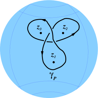
Figure 1: The Pochhammer loop on the Riemann sphere.

Therefore one can consider the Wilson loop

$$W={\rm Tr}\bigg{[}{\cal P}\exp\Big{(}\oint_{\gamma_{P}}{\boldsymbol{A}}\,\Big{)}\,\bigg{]}\ ,$$ (1.16)

whose definition does not depend on the precise shape of the integration contour. In particular, it is not sensitive to deformations of $\gamma_{P}$ which sweep through the monodromy-free punctures. By construction the Wilson loop is an entire function of the spectral parameter $\theta$,

$$\lambda=\rho\ \mbox{e}^{\theta}\ ,\ \ \ \ \ \ {\bar{\lambda}}=\rho\ \mbox{e}^{-\theta}\ .$$ (1.17)

Furthermore, since the shift of the argument $\theta\mapsto\theta+{\rm i}\pi$ does not affect the connection ${\boldsymbol{A}}$, the Wilson loop $W=W(\theta)$ is a periodic function of the period ${\rm i}\pi$. The textbook calculation [28] yields the following asymptotic expansions:

$$\log W\asymp\begin{cases}&-q_{0}\,\rho\mbox{e}^{\theta}+\sum_{n=1}^{\infty}c_{n}\ {\mathfrak{q}}_{2n-1}\ \mbox{e}^{-(2n-1)\theta}\ \ \ {\rm as}\ \ \ \Re e(\theta)\to+\infty,\ \ |\Im m(\theta)|<\frac{\pi}{2}\\ &-q_{0}\,\rho\mbox{e}^{-\theta}+\sum_{n=1}^{\infty}c_{n}\ {\bar{\mathfrak{q}}}_{2n-1}\ \mbox{e}^{(2n-1)\theta}\ \ \ {\rm as}\ \ \ \Re e(\theta)\to-\infty,\ \ |\Im m(\theta)|<\frac{\pi}{2}\end{cases}\ .$$ (1.18)

Here $q_{0}=-\frac{4\pi^{2}}{\prod_{i=1}^{3}\Gamma(1-\frac{a_{i}}{2})}$, whereas $c_{n}=\frac{(-1)^{n}}{2n!}\ \frac{\Gamma(n-\frac{1}{2})}{\sqrt{\pi}}$ stand for the constants that set a conventional multiplicative normalization (see Eqs.(7.13)-(7.16) bellow) for the conserved charges $\{{\mathfrak{q}}_{2n-1},\,{\bar{\mathfrak{q}}}_{2n-1}\}_{n=1}^{\infty}$.

The main result of this work is presented in Section 8, where we conjecture a correspondence between elements of the moduli space ${\cal A}_{\bf m}$ (1.15) and a subset ${\cal H}^{(0)}_{\bf k}$ of the stationary states of the Fateev model in a finite volume. To describe ${\cal H}^{(0)}_{\bf k}$ explicitly, let us recall some basic facts about the model. The Fateev model is governed by the following Lagrangian in $1+1$ Minkowski space

$${\cal L} = \frac{1}{16\pi}\ \sum_{i=1}^{3}\big{(}\,(\partial_{t}\varphi_{i})^{2}-(\partial_{x}\varphi_{i})^{2}\,\big{)}$$

$$+ 2\mu\ \big{(}\,\mbox{e}^{{\rm i}\,\alpha_{3}\varphi_{3}}\ \cos(\alpha_{1}\varphi_{1}+\alpha_{2}\varphi_{2})+\mbox{e}^{-{\rm i}\alpha_{3}\varphi_{3}}\ \cos(\alpha_{1}\varphi_{1}-\alpha_{2}\varphi_{2})\,\big{)}$$

for the three scalar fields $\varphi_{i}=\varphi_{i}(x,t)$. Here $\alpha_{i}$ are coupling constants satisfying the constraint

$$\alpha_{1}^{2}+\alpha_{2}^{2}+\alpha_{3}^{2}=\frac{1}{2}\ .$$ (1.20)

In this work we focus on the case where $\alpha_{i}^{2}>0$. The parameter $\mu$ in the Lagrangian sets the mass scale, $\mu\sim[\,{\rm mass}\,]$. We will consider the theory in a finite-size geometry (where the spatial coordinate $x$ compactified on a circle of circumference $R$) with the periodic boundary conditions

$$\varphi_{i}(x+R,t)=\varphi_{i}(x,t)\ .$$ (1.21)

Due to the periodicity of the potential term in (1) in $\varphi_{i}$, the space of states ${\cal H}$ splits on the orthogonal subspaces ${\cal H}_{k_{1},k_{2},k_{3}}:={\cal H}_{\bf k}$ characterized by the three “quasimomenta” $k_{i}\in[-\frac{1}{2},\frac{1}{2}]$:

$$\varphi_{i}\mapsto\varphi_{i}+2\pi/\alpha_{i}\ :\ \ \ |\,\Psi_{\bf k}\,\rangle\mapsto\mbox{e}^{2\pi{\rm i}k_{i}}\ |\,\Psi_{\bf k}\,\rangle\ ,\ \ \ \ \ \ \ \ |\,\Psi_{\bf k}\,\rangle\in{\cal H}_{\bf k}\ .$$ (1.22)

Similar to the quantum mechanical problem of a particle in a periodic potential, the subspaces ${\cal H}_{\bf k}$ possess the band structure; they split into discrete components labeled by three integers:

$${\cal H}_{\bf k}=\oplus_{n_{1},n_{2},n_{3}\in\mathbb{Z}}\,{\cal H}^{(n_{1},n_{2},n_{3})}_{\bf k}\ .$$ (1.23)

The QFT (1) is integrable, in particular, it has an infinite set of commuting local integrals of motion $\mathbb{I}^{(+)}_{2n-1}$, $\mathbb{I}^{(-)}_{2n-1}$, with $2n=2,\,4,\,6,\,\ldots$ being the Lorentz spins of the associated local densities [21]:

$$\mathbb{I}^{(\pm)}_{2n-1}=\int_{0}^{R}\frac{\mbox{d}x}{2\pi}\ \ \Big{[}\,\sum_{i+j+k=n}C^{(n)}_{ijk}\ (\partial_{\pm}\varphi_{1})^{2i}\,(\partial_{\pm}\varphi_{2})^{2j}\,(\partial_{\pm}\varphi_{3})^{2k}+\ldots\,\Big{]}\ ,$$ (1.24)

where $\partial_{\pm}=\frac{1}{2}(\partial_{x}\mp\partial_{t})$ and $\ldots$ stand for the terms involving higher derivatives of $\varphi_{i}$, as well as the terms proportional to powers of $\mu$. The constant $C^{(n)}_{ijk}$ was found in [23]

$$C^{(n)}_{ijk}=\frac{n!}{i!\ j!\ k!}\ \ \frac{\big{(}2\alpha_{1}^{2}(1-2n)\big{)}_{n-i}\big{(}2\alpha_{2}^{2}\,(1-2n)\big{)}_{n-j}\,\big{(}2\alpha_{3}^{2}\,(1-2n)\big{)}_{n-k}}{(2n-1)^{3}\ (4\alpha^{2}_{1})^{1-i}\ (4\alpha^{2}_{2})^{1-j}\ (4\alpha^{2}_{3})^{1-k}}\ ,$$ (1.25)

where $(x)_{n}$ stands for the Pochhammer symbol. Note, that the displayed terms in (1.24) with $C^{(n)}_{ijk}$ given by (1.25) define the normalization of $\mathbb{I}^{(\pm)}_{2n-1}$ unambiguously. Our primary interest concerns eigenvalues of $\mathbb{I}^{(\pm)}_{2n-1}$ in the subspaces ${\cal H}^{(n_{1},n_{2},n_{3})}_{\bf k}$ (1.23), particularly, in the subspace ${\cal H}^{(0)}_{\bf k}:={\cal H}^{(0,0,0)}_{k_{1},k_{2},k_{3}}$ corresponding to the first Brillouin zone:

$$I^{(\pm)}_{2n-1}\ :\ \ \ \ \ \ \ \mathbb{I}^{(\pm)}_{2n-1}\ |\,\Psi^{(0)}_{\bf k}\,\rangle=I^{(\pm)}_{2n-1}\ |\,\Psi^{(0)}_{\bf k}\,\rangle\ ,\ \ \ \ \ \ \ |\,\Psi^{(0)}_{\bf k}\,\rangle\in{\cal H}^{(0)}_{\bf k}\ .$$ (1.26)

It seems natural to expect that for $0\leq k_{i}\leq\frac{1}{2}$, the sets of eigenvalues $\{I^{(+)}_{2n-1},I^{(-)}_{2n-1}\}_{n=1}^{\infty}$ fully specify the common eigenbasis of the local IM in ${\cal H}^{(0)}_{\bf k}$.

In the recent paper [29] it was argued that the vacuum eigenvalues $\{I^{(+)}_{2n-1},I^{(-)}_{2n-1}\}_{n=1}^{\infty}$ (i.e. those corresponding to the unique state in ${\cal H}^{(0)}_{\bf k}$ with the lowest value of the energy $E=I^{(+)}_{1}+I^{(-)}_{1}$) are simply related to the set of conserved charges $\{{\mathfrak{q}}_{2n-1},\,{\bar{\mathfrak{q}}}_{2n-1}\}_{n=1}^{\infty}$ associated with the unique element ${\cal A}^{(0,0)}_{\bf m}$ of the moduli space ${\cal A}_{\bf m}$ (1.15). Namely:

$$\mu^{-1}\ \big{(}\,I_{1}-{\textstyle\frac{1}{2}}\,R\,{\cal E}_{0}\,\big{)}=d_{1}\ {\mathfrak{q}}_{1}\ ,\ \ \ \ \ \ \ \ \ \ \mu^{-1}\ \big{(}\,{\bar{I}}_{1}-{\textstyle\frac{1}{2}}\,R\,{\cal E}_{0}\,\big{)}=d_{1}\ {\bar{\mathfrak{q}}}_{1}$$ (1.27)

and

$$\mu^{1-2n}\ I^{(+)}_{2n-1}=d_{n}\ {\mathfrak{q}}_{2n-1}\ ,\ \ \ \ \ \ \ \ \ \ \ \ \mu^{1-2n}\ I^{(-)}_{2n-1}=d_{n}\ {\bar{\mathfrak{q}}}_{2n-1}\ \ \ \ \ \ \ \ \ \ \ \ \ (n=2,\,3,\,\ldots)\ .$$ (1.28)

With the normalization conditions described above, the constants $d_{n}$ and ${\cal E}_{0}$ reads explicitly as

$$d_{n}=(2\pi)^{2n-1}\ \ \frac{(-1)^{n-1}}{16\,\pi^{2}}\ \ \prod_{i=1}^{3}\Gamma\big{(}\,2\,(2n-1)\,\alpha^{2}_{i}\,\big{)}$$ (1.29)

and

$${\cal E}_{0}=-\pi\mu^{2}\ \prod_{i=1}^{3}\frac{\Gamma(2\alpha_{i}^{2})}{\Gamma(1-2\alpha_{i}^{2})}\ .$$ (1.30)

These relations should be supplemented by the identification of the parameters from the quantum and classical integrable problems:

$$\alpha_{i}^{2}={\frac{a_{i}}{4}}\,,\ \ \ \ \ \ \ \qquad k_{i}=\frac{1}{a_{i}}\ (2m_{i}+1)\ \ \ \ \ \qquad(i=1,2,3)\ ,$$ (1.31)

whereas the relation between dimensionless parameter $\mu R$ and $\rho$ is given by

$$\mu R=2\rho\ .$$ (1.32)

In this work we promote Eqs.(1.27)-(1.32) to a general relations between the joint spectra of the local IM in the subspace ${\cal H}^{(0)}_{\bf k}$ corresponding the first Brillouin zone and the set of the conserved charges associated with the elements of the moduli space ${\cal A}_{\bf m}$. For the values of $k_{i}$ restricted to the segment $[\,0,\frac{1}{2}\,]$, this gives a remarkable bijection between the joint eigenbasis of the local IM in ${\cal H}^{(0)}_{\bf k}$ and the elements of ${\cal A}_{\bf m}$.

In Section 9 we demonstrate that the correspondence between the classical and quantum integrable systems provides a powerful tool for deriving integral equations which determine the full spectrum of local IM in the massive QFT.

We conclude this paper with few remarks concerning the QFT (1) in the regime where one of the couplings $\alpha_{i}$ is pure imaginary.

2 Generalized Hypergeometric Oper

2.1 Monodromies of the Fuchsian differential equations

In this preliminary subsection we include some basic concepts and results about the Fuchsian differential equations.

Let $z$ stands for the complex coordinate on $\mathbb{CP}^{1}\backslash\{z_{1},z_{2},\ldots z_{n}\}$, the Riemann sphere with $n$ punctures. Consider the second order Fuchsian differential operator $-\partial_{z}^{2}+T(z)$, where $T(z)$ is given by

$$T(z)=-\sum_{i=1}^{n}\Big{(}\,\frac{\delta_{i}}{(z-z_{i})^{2}}+\frac{c_{i}}{z-z_{i}}\,\Big{)}\ .$$ (2.1)

The equation

$$\big{(}-\partial_{z}^{2}+T(z)\,\big{)}\,\psi=0$$ (2.2)

is a general second-order differential equation with $n$ regular singular points. We will always regard the parameters $\delta_{i}$ as fixed numbers. The positions of the singularities $z_{i}$ and the coefficients $c_{i}$ (which are usually referred to as the “accessory parameters”) will be treated as variables. The accessory parameters $c_{i}$ are constrained by the elementary relations

$$\sum_{i=1}^{n}c_{i}=0\ ,\ \ \ \ \ \sum_{i=1}^{n}(z_{i}\,c_{i}+\delta_{i})=0\ ,\ \ \ \ \sum_{i=1}^{n}(z_{i}^{2}\,c_{i}+2\,z_{i}\delta_{i})=0\ ,$$ (2.3)

ensuring that $T(z)$ has no additional singularity at $z=\infty$. Thus only $n-3$ of these parameters are independent. Also, the projective transformations of the variable $z$ allows one to send three of the points $z_{i}$, say $(z_{1},\,z_{2},\,z_{3})$, to any designated positions, usually $(0,\,1,\,\infty)$. Therefore, with fixed $\delta_{i}$, the differential equation (2.2) essentially depends on $2\,(n-3)$ complex parameters.

The equation (2.2) generates a monodromy group — a homomorphism of the fundamental group of the sphere with marked points into the group $\mathbb{SL}(2,\mathbb{C})$,

$${\boldsymbol{M}}\ :\ \ \pi_{1}\big{(}\mathbb{CP}^{1}\backslash\{z_{i}\}\big{)}\mapsto\mathbb{SL}(2,\mathbb{C})\ .$$ (2.4)

Let $(\psi_{1}(z),\psi_{2}(z))$ is a basis of linearly independent solutions of (2.2). Then its continuation along any closed path $\gamma$ defines the monodromy matrix

$${\boldsymbol{M}(\gamma)}\ :\ \ \ \ \ \big{(}\psi_{1}(\gamma\circ z),\psi_{2}(\gamma\circ z))=(\psi_{1}(z),\psi_{2}(z))\,{\boldsymbol{M}}(\gamma)\ ,$$ (2.5)

which depends only on the homotopy class of $\gamma\in\pi_{1}(\mathbb{CP}^{1}\,\backslash\{z_{i}\})$. Let $\gamma_{i}\in\pi_{1}(\mathbb{CP}^{1}\backslash\{z_{i}\}),\ i=1,2,\ldots n$ be the elementary paths around the points $z_{i}$, and

$${\boldsymbol{M}}^{(i)}:={\boldsymbol{M}}(\gamma_{i})\in\mathbb{SL}(2,\mathbb{C})$$ (2.6)

the associated elements of the monodromy group of (2.2). The parameters

$$\delta_{i}=\delta(p_{i})\ \ \ \ \ \ \ \ \ {\rm with}\ \ \ \ \ \ \ \ \ \ \ \delta(p)={\textstyle\frac{1}{4}}-p^{2}$$ (2.7)

determine the conjugacy classes of ${\boldsymbol{M}}^{(i)}$ via the equation

$${\rm Tr}\big{(}{\boldsymbol{M}}^{(i)}\big{)}=-2\,\cos(2\pi p_{i})\ .$$ (2.8)

Let $\big{\{}\Gamma_{a}\big{\}}_{a=1}^{n-3}$ be the system of contours shown in Fig. 2, such that $\Gamma_{a}$ loops around the punctures $z_{1},\,z_{4},\ldots z_{3+a}$ only;

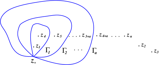
Figure 2: The elements $\Gamma_{1},\,\Gamma_{2},\ldots\Gamma_{n-3}$ of the fundamental group $\pi_{1}\big{(}\mathbb{CP}^{1}\backslash\{z_{i}\}\big{)}$. Choosing the accessory parameters in (2.1) according to (2.11) fixes the conjugacy classes of the associated elements of the monodromy group of (2.2) as given in (2.9).

and let the set ${\boldsymbol{\nu}}=(\nu_{1},\ldots\nu_{n-3})$ parameterize the conjugacy classes of the corresponding monodromy matrices ${\boldsymbol{M}}(\Gamma_{a})$,

$${\rm Tr}\big{(}\,{\boldsymbol{M}}(\Gamma_{a})\,\big{)}=-2\ \cos(\pi\nu_{a})\ \ \ \ \ (a=1,\ldots n-3)\ .$$ (2.9)

For given conjugacy classes (2.9) (i.e., for a given set ${\boldsymbol{\nu}}$), the accessory parameters are determined in terms of the so-called classical conformal block $f_{\boldsymbol{\nu}}(X_{1},\ldots X_{n-3})$ corresponding to “haircomb” diagram shown in Fig. 3 (for details, see e.g.[30, 31]). Namely,

$$c_{i}=\frac{\partial}{\partial z_{i}}\ F\ \ \ \ \ \ \ \ \ \ \ \ \ (i=1,\ldots n)\ ,$$ (2.10)

where the shortcut notation $F$ stands for

$$F=F_{0}+\delta_{3}\ \log\Big{(}\frac{z_{21}}{z_{31}z_{32}}\Big{)}+\sum_{i=1\atop i\not=3}^{n}\delta_{i}\ \log\Big{(}\frac{z_{31}z_{32}}{z_{21}z^{2}_{3i}}\Big{)}+f_{\boldsymbol{\nu}}(X_{1},\ldots X_{n-3})\ ,$$ (2.11)

with $z_{ij}:=z_{i}-z_{j}$ and the arguments of the conformal block are cross ratios

$$X_{a}=\frac{z_{a+3}-z_{1}}{z_{a+3}-z_{3}}\ \frac{z_{2}-z_{3}}{z_{2}-z_{1}}\ \ \ \ \ \ \ \ \ (a=1,\ldots n-3)\ .$$ (2.12)

A certain additive normalization of the classical conformal block is usually assumed. For this reason, we reserve the room for an arbitrary coordinate-independent constant $F_{0}$ in (2.11).

Figure 3: Dual diagram for the classical conformal block from Eq.(2.11), $\delta(\nu_{a}/2)=\frac{1}{4}\,(1-\nu_{a}^{2})$.

2.2 Definition of GHO

Here we consider a special class of second order Fuchsian differential operators. We will always assume that the three parameters $p_{i}$ defining conjugacy classes of the matrices ${\boldsymbol{M}}^{(i)}$ in (2.6)-(2.8), associated with the elementary paths around the “fixed” punctures $z_{1},\,z_{2},\ z_{3}$, are positive numbers satisfying the following constraints

$$0<p_{i}<{\textstyle\frac{1}{2}}\ \ \ (i=1,\,2,\,3)\ ,\ \ \ \ \ 0<p_{1}+p_{2}+p_{3}<{\textstyle\frac{1}{2}}\ .$$ (2.13)

For the remaining $L:=n-3$ punctures we require that both linearly independent solutions of (2.2) are single-valued (or monodromy-free) in the vicinity of these punctures. It is well known [32] how to reformulate this condition as a set of algebraic relations imposed on the corresponding parameters $\delta_{3+a}$, $C_{a}:=c_{3+a}$   and $x_{a}:=z_{3+a}$, $(a=1,\ldots L)$. Namely, suppose that $T(z)$ has a Laurent expansion at $z=x_{a}$ of the form

$$T(z)=-\frac{l_{a}(l_{a}+1)}{(z-x_{a})^{2}}-\frac{C_{a}}{z-x_{a}}-\sum_{k=0}^{+\infty}t^{(a)}_{k}\ (z-x_{a})^{k}\ .$$ (2.14)

It is easy to see that $l_{a}$ must be an integer. We will focus on the case $l_{a}=1$, i.e.

$$\delta_{3+a}=-2\ \ \ \ \ \ (a=1,\ldots L)\ .$$ (2.15)

To ensure that solutions of Eq.(2.2) are single-valued in the vicinity of the punctures at $z=x_{a}\ (a=1,\ldots L)$, the expansion coefficients $t^{(a)}_{0}$ and $t^{(a)}_{1}$ in (2.14) should be constrained as

$$(C_{a})^{3}\,-4\ C_{a}\ t^{(a)}_{0}+4\,t^{(a)}_{1}=0\ .$$ (2.16)

This yields

$$C_{a}\ \bigg{[}\,\frac{1}{4}\ (C_{a})^{2}-T_{0}(x_{a})-\sum_{b\not=a}^{L}\Big{(}\frac{2}{(x_{a}-x_{b})^{2}}-\frac{C_{b}}{x_{a}-x_{b}}\,\Big{)}\bigg{]}$$

$$-T^{\prime}_{0}(x_{a})+\sum_{b\not=a}^{L}\Big{(}\frac{4}{(x_{a}-x_{b})^{3}}-\frac{C_{b}}{(x_{a}-x_{b})^{2}}\,\Big{)}=0\ \ \ \ \ (a=1,\ldots L)\ ,$$ (2.17)

where

$$T_{0}(z)=-\sum_{i=1}^{3}\Big{(}\,\frac{\delta_{i}}{(z-z_{i})^{2}}+\frac{c_{i}}{z-z_{i}}\,\Big{)}\ .$$ (2.18)

The prime in $T^{\prime}(z)$ stands for the derivative w.r.t. the variable $z$. This system of algebraic equations should be supplemented by the three conditions (2.3), specialized to the case (2.15):

$$\sum_{i=1}^{3}c_{i} = -\sum_{a=1}^{L}C_{a}\ ,$$

$$\sum_{i=1}^{3}(z_{i}\,c_{i}+\delta_{i}) = -\sum_{a=1}^{L}(x_{a}\,C_{a}-2)\ ,$$ (2.19)

$$\sum_{i=1}^{3}(z_{i}^{2}\,c_{i}+2x_{i}\delta_{i}) = -\sum_{a=1}^{L}(x^{2}_{a}\,C_{a}-4x_{a})\ .$$

As far as positions of the punctures $z_{1},z_{2},z_{3}$ and corresponding parameters ${\bf p}=(p_{1},\,p_{2},\,p_{3})$ are fixed, Eqs.(2.2), (2.2) define an algebraic variety which will be denoted by ${\cal V}^{(L)}_{\bf p}$. If positions of the punctures $(x_{1},\ldots x_{L})$ are used as local coordinates on ${\cal V}^{(L)}_{\bf p}$, then a system of $L$ locally defined functions $C_{a}(x_{1},\ldots x_{L})$ satisfy the integrability conditions

$$\frac{\partial}{\partial x_{b}}\,C_{a}=\frac{\partial}{\partial x_{a}}\,C_{b}\ .$$ (2.20)

These relations can be verified by the brute-force calculation using Eqs.(2.2) and (2.2), but, of course, they follows immediately from the general relation (2.10). In this particular case the classical conformal block in Eq.(2.11) is related to the classical limit of the $(3+L)$-point correlator involving three generic chiral vertex operators $V_{i}$ with conformal dimensions $\Delta_{i}\ (i=1,2,3)$ and $L$ degenerate vertices $V_{(3,1)}$ with dimensions $\Delta_{(3,1)}$:

$$\langle\,V_{1}(0)\,V_{2}(1)\,V_{3}(\infty)\,V_{(3,1)}(X_{1})\,\ldots\,V_{(3,1)}(X_{L})\,\rangle\sim\exp\Big{(}\,\frac{1}{b^{2}}\ f_{\boldsymbol{\nu}}(X_{1},\ldots X_{L})\,\Big{)},\quad b^{2}\to 0\,,$$ (2.21)

where the parameter $b^{2}$ and other conventional notations are inherited from the quantum Liouville theory (see Ref.[33] for details)

$$\Delta_{i}\to\frac{\delta_{i}}{b^{2}}\ ,\ \ \ \ \ \Delta_{(3,1)}\to-\frac{2}{b^{2}}\ \ \ \ {\rm as}\ \ \ \ \ b^{2}\to 0\ .$$ (2.22)

Due to the well known fusion rule for the degenerate vertex $V_{(3,1)}$ [34], only a discrete set of the parameters ${\boldsymbol{\nu}}=(\nu_{1},\ldots\nu_{L})$ is allowed (see Fig. 4):

$$\nu_{1}=2\,(p_{1}+\epsilon_{1})\ ,\ \ \ \ \ \nu_{a}=\nu_{a-1}+2\,\epsilon_{a}\ \ \ \ \ \ \ (a=2,\ldots L)\ ,$$ (2.23)

where the discrete variables $\epsilon_{a}$ takes the values $0,\pm 1$ only.

\psfrag{z1}{$(0,\delta_{1})$}\psfrag{z2}{$(X_{1},-2)$}\psfrag{z3}{$\delta(p_{1}+\epsilon_{1})$}\psfrag{z4}{$(X_{2},-2)$}\psfrag{z5}{$\delta(p_{1}+\epsilon_{1}+\epsilon_{2})$}\psfrag{z6}{$(X_{L},-2)$}\psfrag{z7}{${\textstyle\delta(p_{1}+\epsilon_{1}+\ldots+\epsilon_{L})}$}\psfrag{z8}{$(1,\delta_{2})$}\psfrag{z9}{$(\infty,\delta_{3})$}\psfrag{zz}{$\cdots$}\includegraphics[width=426.79134pt]{block_GHOc.eps}

Figure 4: Dual diagram for the classical conformal block from Eq.(2.21). Here $\epsilon_{a}=0,\,\pm 1$ $(a=1,\ldots L).$

Different configurations $(\epsilon_{1},\ldots\epsilon_{L})$ correspond to the different locally defined functions $C^{(\epsilon_{1}\ldots\epsilon_{L})}_{a}(x_{1},\ldots x_{L})\ (\epsilon_{a}=0,\pm 1)$, which are branches of the multivalued algebraic function of the complex variables $x_{1},\ldots x_{L}$. This is illustrated by the simplest case with $L=1$ in Appendix A.

In what follows we will refer to the differential operators (1.1), whose moduli space coincides with the algebraic variety ${\cal V}^{(L)}_{\bf p}$ as to the Generalized Hypergeometric Opers (GHO’s). The marked points $x_{a}\ (a=1,\ldots L)$ will be called as monodromy-free punctures.

2.3 Connection matrices for GHO

We have introduced the concept of GHO because the monodromy group of such opers coincides with the monodromy group of the conventional hypergeometric equation. Let us recall some facts about this group. In the case under consideration there are only three elementary $\mathbb{SL}(2,{\mathbb{C}})$-matrices ${\boldsymbol{M}}^{(i)}$, ${\boldsymbol{M}}^{(j)}$ and ${\boldsymbol{M}}^{(k)}$ (2.8), corresponding to the contours $\gamma_{i}$, $\gamma_{j}$ and $\gamma_{k}$, shown in Fig. 5. Here $(i,j,k)$ is any cyclic permutation of $(1,2,3)$.

Figure 5: The contractible loop $\gamma_{k}\circ\gamma_{j}\circ\gamma_{i}=\gamma_{i}\circ\gamma_{k}\circ\gamma_{j}=\gamma_{j}\circ\gamma_{i}\circ\gamma_{k}$ on the sphere with three punctures.

These matrices satisfy an obvious relation

$${\boldsymbol{M}}^{(i)}{\boldsymbol{M}}^{(k)}{\boldsymbol{M}}^{(j)}={\boldsymbol{I}}\ ,$$ (2.24)

because the contour $\gamma_{i}\circ\gamma_{k}\circ\gamma_{j}$ is a contractible loop. Further, since $0<p_{i}<\frac{1}{2}$, one of these matrices, say, ${\boldsymbol{M}}^{(i)}$ can always be chosen diagonal

$${\boldsymbol{M}}^{(i)}=-\mbox{e}^{-2\pi{\rm i}p_{i}\sigma_{3}}\ .$$ (2.25)

Here and below we use standard notation for the Pauli matrices $\sigma_{1},\sigma_{2},\sigma_{3}$. Then Eqs.(2.8), (2.24), (2.25) define ${{\boldsymbol{M}}}^{(j)}$ and ${{\boldsymbol{M}}}^{(k)}$ up to a diagonal similarity transformation. In particular,

$${{\boldsymbol{M}}}^{(j)}=\mbox{e}^{-\omega_{i}\sigma_{3}}\ \Bigg{[}\ \frac{{\rm i}}{s(2p_{i})}\ \begin{pmatrix}\mbox{e}^{2\pi{\rm i}p_{i}}\ c(2p_{j})+\,c(2p_{k})&2\,\Lambda\\ -2\ \Lambda&-\mbox{e}^{-2\pi{\rm i}p_{i}}\,c(2p_{j})-\,c(2p_{k})\end{pmatrix}\ \Bigg{]}\ \mbox{e}^{\omega_{i}\sigma_{3}}\ .$$ (2.26)

The quantity $\omega_{i}$ is an arbitrary complex number and

$$\Lambda=\sqrt{c(p_{2}+p_{3}-p_{1})\,c(p_{1}+p_{2}-p_{3})c(p_{1}-p_{2}+p_{3})\,c(p_{1}+p_{2}+p_{3})}\ ,$$ (2.27)

where we have used the shorthand notations

$$c(p)=\cos(\pi p)\ ,\ \ \ \ \ \ \ \ \ s(p)=\sin(\pi p)\ .$$ (2.28)

We now return to the the equation (2.2) corresponding to the GHO. Let $\chi^{(i)}_{\sigma}(z)$ $(i=1,2,3;\ \sigma=\pm)$ be its solutions such that

$$\chi_{\sigma}^{(i)}\to\frac{1}{\sqrt{2p_{i}}}\ (z-z_{i})^{\frac{1}{2}+\sigma p_{i}}\,\Big{(}1+O(z-z_{i})\Big{)}\qquad{\rm as}\ \ \ \ \ \ \ \ \ z\to z_{i}\ .$$ (2.29)

The prefactor here is chosen to satisfy the normalization condition

$${\tt W}[\chi_{\sigma^{\prime}}^{(i)},\,\chi_{\sigma}^{(i)}]=\sigma\,\delta_{\sigma+\sigma^{\prime},0}\ ,$$ (2.30)

where ${\tt W}[f,g]=fg^{\prime}-gf^{\prime}$ stands for the Wronskian. If the constraints (2.13) are imposed, the asymptotic conditions (2.29) define three different bases (for $i=1,2,3$) in the two-dimensional linear space of solutions of (2.2). Let us combine the solutions (2.29) for given $i$ into the row

$${\boldsymbol{\chi}}^{(i)}=(\chi_{-}^{(i)},\chi_{+}^{(i)})\,,\qquad i=1,2,3\ .$$ (2.31)

Then the two sets of basis vectors ${\boldsymbol{\chi}}^{(i)}$ and ${\boldsymbol{\chi}}^{(j)}$ are related through a linear transformation

$${\boldsymbol{\chi}}^{(i)}={\boldsymbol{\chi}}^{(j)}\ {\boldsymbol{S}}^{(j,i)}\ .$$ (2.32)

Here ${\boldsymbol{S}}^{(j,i)}$ stand for $\mathbb{SL}(2,\mathbb{C})$-matrices, satisfying the relations

$$\det\big{(}{\boldsymbol{S}}^{(j,i)}\big{)}=1\,,\qquad{\boldsymbol{S}}^{(i,k)}{\boldsymbol{S}}^{(k,i)}={\boldsymbol{I}}\,,\qquad{\boldsymbol{S}}^{(i,k)}{\boldsymbol{S}}^{(k,j)}{\boldsymbol{S}}^{(j,i)}={\boldsymbol{I}}\,,$$ (2.33)

where again $(i,j,k)$ is any cyclic permutation of $(1,2,3)$. It is easy to see that one needs six independent complex numbers to parameterize the three matrices ${\boldsymbol{S}}^{(i+1,i)}$ $(i\sim i+3)$ satisfying (2.33). Moreover, these connection matrices are subject to three additional complex constraints. Indeed, the monodromy matrix ${\boldsymbol{M}}^{(j)}$ (2.26) can be expressed in term of the connection matrix ${\boldsymbol{S}}^{(j,i)}$:

$${\boldsymbol{M}}^{(j)} = -\big{(}{\boldsymbol{S}}^{(j,i)}\big{)}^{-1}\ \mbox{e}^{-2\pi{\rm i}p_{j}\sigma_{3}}\ {\boldsymbol{S}}^{(j,i)}\ .$$ (2.34)

This relation combined with Eqs.(2.33) leads to

$${\boldsymbol{S}}^{(j,i)}=-\mbox{e}^{-\omega_{j}\sigma_{3}}\ \mbox{e}^{{\rm i}\pi p_{j}\sigma_{3}}\ \sigma_{2}\ {\boldsymbol{A}}^{(k)}\ \mbox{e}^{\omega_{i}\sigma_{3}}\ ,$$ (2.35)

with

$${\boldsymbol{A}}^{(k)}=\begin{pmatrix}A^{(k)}_{--}&A^{(k)}_{-+}\\ A^{(k)}_{+-}&A^{(k)}_{++}\end{pmatrix}\ ,$$ (2.36)

where the matrix elements read explicitly

$$A_{\sigma^{\prime}\sigma}^{(k)}=\sqrt{\frac{\Lambda}{s(2p_{i})s(2p_{j})}}\ \ \bigg{[}\,\frac{c(p_{i}+p_{j}+p_{k})\,c(p_{i}+p_{j}-p_{k})}{c(p_{i}-p_{j}+p_{k})\,c(p_{i}-p_{j}-p_{k})}\,\bigg{]}^{\frac{\sigma\sigma^{\prime}}{4}}$$ (2.37)

and $\Lambda$ is given by (2.27). Note that Eq.(2.35) can be equivalently rewritten as a formula for the Wronskians:

$${\tt W}[\chi_{\sigma^{\prime}}^{(j)},\chi_{\sigma}^{(i)}]=-{\rm i}\ \mbox{e}^{{\rm i}\pi\sigma^{\prime}p_{j}}\ \ A_{\sigma^{\prime}\sigma}^{(k)}\ \mbox{e}^{-\sigma^{\prime}\omega_{j}-\sigma\omega_{i}}\ .$$ (2.38)

The complex parameters $\omega_{i}\ (i=1,2,3)$, entering the expression (2.35), remain undetermined. These parameters do not affect the conjugacy class of the representation of $\pi_{1}\big{(}\mathbb{CP}^{1}\backslash\{z_{1},z_{2},z_{3}\}\big{)}$. Nevertheless, they are important characteristics of the GHO itself. In the next section we argue that, in the case of GHO, a coordinate-independent additive normalization of the function $F$ (2.11) can be chosen in such a way that

$$\exp(\omega_{i})=\exp\Big{(}-\frac{1}{2}\ \frac{\partial}{\partial p_{i}}\ F\,\Big{)}\ \ \ \ \ \ \ \ \ \ (i=1,2,3)\ .$$ (2.39)

An immediate consequence of this fact is that

$$\exp(\omega_{i})\ \Big{(}\frac{z_{jk}}{z_{ji}z_{ik}}\Big{)}^{-p_{i}}$$ (2.40)

depends on $L$ projective invariants (2.12) only. Explicit forms for (2.40) in the cases $L=0$ and $L=1$ are given by equations (B.2) and (B.4) from Appendix B, respectively.

Finally, note that $\exp({\omega_{i})}$ is defined up to the phase factor $\pm\mbox{e}^{2\pi{\rm i}pM}\ (M\in\mathbb{Z})$. This ambiguity is inherited from the similar ambiguity in the definition of $\chi_{\sigma}^{(i)}$ in Eq.(2.29).

2.4 GHO and complex solutions of the Liouville equation

Until now we have discussed holomorphic GHO only. Of course, with minor modifications all the above can applied to the antiholomorphic GHO

$${\bar{\cal D}}=-\partial_{\bar{z}}^{2}-\sum_{i=1}^{3}\Big{(}\,\frac{{\bar{\delta}}_{i}}{({\bar{z}}-{\bar{z}}_{i})^{2}}+\frac{{\bar{c}}_{i}}{{\bar{z}}-{\bar{z}}_{i}}\,\Big{)}-\sum_{b=1}^{\bar{L}}\Big{(}\,\frac{(-2)}{({\bar{z}}-{\bar{y}}_{b})^{2}}+\frac{{\bar{C}}_{b}}{{\bar{z}}-{\bar{y}}_{b}}\,\Big{)}\ .$$ (2.41)

In what follows we assume that the triple $\{{\bar{z}}_{i}\}_{i=1}^{3}$ is complex conjugate to $\{z_{i}\}_{i=1}^{3}$, the corresponding ${\bar{\delta}}_{i}=\delta_{i}$ are real and, furthermore,

$$p_{i}={\bar{p}}_{i}\ .$$ (2.42)

We will not impose any relations between coordinates of the monodromy-free punctures for the holomorphic and antiholomorphic GHO’s. For this reason the coordinates of antiholomorphic monodromy-free punctures in (2.41) are denoted by ${\bar{y}}_{b}\,,\ b=1,\ldots{\bar{L}}$ and ${\bar{L}}=0,1,2\ldots$ does not necessarily coincide with $L$.

Let ${\bar{\chi}}_{\sigma}^{(i)}$ be the basis solutions of ${\bar{\cal D}}{\bar{\psi}}=0$, which are defined similarly to Eq.(2.29). With the same arguments as above, one arrives to the antiholomorphic analog of Eq.(2.38)

$${\tt W}[{\bar{\chi}}_{\sigma^{\prime}}^{(j)},{\bar{\chi}}_{\sigma}^{(i)}]={\rm i}\ \mbox{e}^{-{\rm i}\pi\sigma^{\prime}p_{j}}\ \ A_{\sigma^{\prime}\sigma}^{(k)}\ \mbox{e}^{-\sigma^{\prime}{\bar{\omega}}_{j}-\sigma{\bar{\omega}}_{i}}\ ,$$ (2.43)

where $A_{\sigma^{\prime}\sigma}^{(k)}$ is the same matrix as in Eq.(2.37).

Consider a bilinear form

$$\tau(z,{\bar{z}})={\boldsymbol{\chi}}^{(i)}\ {\boldsymbol{G}}^{(i)}\ \big{(}\bar{{\boldsymbol{\chi}}}^{(i)}\big{)}^{T}$$ (2.44)

where ${\boldsymbol{G}}^{(i)}$ is an arbitrary $2\times 2$ matrix and superscript $T$ stands for the matrix transposition. We specialize ${\boldsymbol{G}}^{(i)}$ by the requirement that $\tau(z,{\bar{z}})$ is a single-valued function on the punctured sphere. Imposing this condition in the vicinity of the puncture $z_{i}$, one concludes that ${\boldsymbol{G}}^{(i)}$ is a diagonal matrix. With the connection formula (2.32), the single-valuedness implies that ${\boldsymbol{S}}^{(ji)}\ {\boldsymbol{G}}^{(i)}\ \big{(}{\bar{\boldsymbol{S}}}^{(ji)}\big{)}^{T}$ is also a diagonal matrix. Using the explicit form of connection matrices (2.35)-(2.37), one finds

$${\boldsymbol{G}}^{(i)}={\rm const}\ \mbox{e}^{-(\omega_{i}+{\bar{\omega}}_{i})\sigma_{3}}\ \sigma_{3}\ .$$ (2.45)

If the undetermined constant is chosen to be $\pm 1$, then the complex function

$$\eta\ :\ \ \ \ \ \mbox{e}^{-\eta}:=\tau(z,{\bar{z}})\ ,$$ (2.46)

satisfies the Liouville equation

$$\partial_{z}\partial_{\bar{z}}\eta=\mbox{e}^{2\eta}\ .$$ (2.47)

This fact can be easily verified and it is well known in the theory of the classical Liouville equation. Since we are considering the complex solution of Eq.(2.47), the overall sign of the constant in (2.45) it is not important and we fix it to be $1$. As a result, one has

$$\mbox{e}^{-\eta}=\mbox{e}^{-(\omega_{i}+{\bar{\omega}}_{i})}\ \ \chi_{-}^{(i)}{\bar{\chi}}_{-}^{(i)}-\mbox{e}^{\omega_{i}+{\bar{\omega}}_{i}}\ \chi_{+}^{(i)}{\bar{\chi}}_{+}^{(i)}\ .$$ (2.48)

At the monodromy-free punctures, $z=x_{a}\ (a=1,\ldots L)$ and ${\bar{z}}={\bar{y}}_{b}\ (b=1,\ldots{\bar{L}})$, $\mbox{e}^{-\eta}$ becomes singular,

$$\mbox{e}^{-\eta}\sim\frac{1}{z-x_{a}}\ \ \ \ \ \ {\rm and}\ \ \ \ \ \ \ \mbox{e}^{-\eta}\sim\frac{1}{{\bar{z}}-{\bar{y}}_{b}}\ ,$$ (2.49)

however it still remains single-valued. Thus, $\mbox{e}^{-\eta}$ is a complex single-valued function on the sphere with $3+L+{\bar{L}}$ punctures. Notice, that it does not have any zeroes, as this contradicts to the Liouville equation (2.47).

As it follows from Eq.(2.48), the solution $\eta$ satisfies the asymptotic conditions

$$\eta = -2\ \log|z|+O(1)\ \ \ \ \ \ \ \ \ \ \ \,\ \ \ \ \ \ \ \ \ \ \ \ \ \ \ \ \ \ \ \ {\rm as}\ \ \ \ \ \ |z|\to\infty$$

$$\eta = 2\,m_{i}\ \log|z-z_{i}|+\eta^{\rm(reg)}_{i}+o(1)\ \ \ \ \ \ \ \ \ \ \ \ \ \ \ {\rm as}\ \ \ \ \ \ |z-z_{i}|\to 0\ ,$$ (2.50)

where

$$m_{i}=p_{i}-\frac{1}{2}\ ,\ \ \ \ \ \ \ \ \ \ \ \ \ \ \frac{\exp\big{(}\eta^{\rm(reg)}_{i}\big{)}}{2\,p_{i}}=\mbox{e}^{\omega_{i}+{\bar{\omega}}_{i}}\ .$$ (2.51)

The constants $\eta^{\rm(reg)}_{i}$ can be regarded as regularized values of the Liouville field at the punctures $z_{i}$. They are be expressed in terms of the regularized Liouville action [36, 33]. To explain this important relation we recall that the Liouville equation and the asymptotic conditions (2.4) follow from the variational principle for the functional

$${\cal A}_{\rm Liouv}[\eta] = \lim_{\epsilon_{i}\to 0\atop R\to\infty}\,\bigg{[}\,\frac{1}{\pi}\ \int_{|z-z_{i}|>\epsilon\atop|z|<R}\mbox{d}^{2}z\ \big{(}\,\partial_{z}{\eta}\partial_{\bar{z}}{\eta}+\mbox{e}^{2\eta}\,\big{)}$$

$$+ 2\ \sum_{i=1}^{3}\big{(}\,m_{i}\,\eta_{i}-m_{i}^{2}\,\log(\epsilon_{i})\,\big{)}+2\,\eta_{\infty}+2\,\log R\,\bigg{]}\ .$$

Since the fields configuration is singular at $z\to z_{i}$, we cut out a small disk of radius $\epsilon_{i}$ around the point $z_{i}$ and add the boundary terms with

$$\eta_{i}=\frac{1}{2\pi\epsilon_{i}}\ \oint_{|z-z_{i}|=\epsilon_{i}}\mbox{d}\ell\,\eta$$ (2.53)

to ensure the behavior (2.4) near $z_{i}$. To control the large $|z|$-behavior we regularize the action for large values of $z$ and add the boundary term with

$$\eta_{\infty}=\frac{1}{2\pi R}\ \oint_{|z|=R}\mbox{d}\ell\,\eta\ .$$ (2.54)

In addition, we include some field independent terms such that ${\cal A}_{\rm Liouv}$ is finite and independent on $\epsilon_{i}$ and $R$ when $\epsilon_{i}\to 0$, $R\to\infty$. Contributions of the monodromy-free punctures (2.49) to the functional (2.4) are finite and therefore there is no need to include additional regularization terms to the action. It is now easy to show that

$$\eta^{\rm(reg)}_{i}=\frac{1}{2}\ \frac{\partial{\cal A}_{\rm Liouv}^{*}}{\partial p_{i}}\ ,$$ (2.55)

where ${\cal A}^{*}_{\rm Liouv}$ stands for the stationary value of the functional (2.4) calculated on the field configuration $\eta$ defined by Eq.(2.48). More generally, the stationary value of the Liouville functional depends on $6+L+{\bar{L}}$ variables,

$${\cal A}^{*}_{\rm Liouv}={\cal A}^{*}_{\rm Liouv}\big{(}\,p_{1},p_{2},p_{3}\,|\,z_{1},z_{2},z_{3};x_{1},\ldots x_{L};{\bar{y}}_{1},\ldots{\bar{y}}_{\bar{L}}\,\big{)}\ ,$$ (2.56)

and its total deferential is given by [36, 33]

$$\mbox{d}{\cal A}^{*}_{\rm Liouv}=2\sum_{i=1}^{3}\eta_{i}\,\mbox{d}p_{i}-\sum_{i=1}^{3}\big{(}c_{i}\,\mbox{d}z_{i}+{\bar{c}}_{i}\,\mbox{d}{\bar{z}}_{i}\big{)}-\sum_{a=1}^{L}C_{a}\,\mbox{d}x_{a}-\sum_{b=1}^{\bar{L}}{\bar{C}}_{b}\,\mbox{d}{\bar{y}}_{b}\ .$$ (2.57)

As it follows from (2.10), ${\cal A}^{*}_{\rm Liouv}$ can be expressed in terms of $F$ and its antiholomorphic counterpart ${\bar{F}}$:

$${\cal A}^{*}_{\rm Liouv}=-F-{\bar{F}}\ .$$ (2.58)

The coordinate-independent constant $F_{0}$ in Eq.(2.11) has not yet been fixed. Therefore there is no need to add a $p_{i}$-dependent constant in (2.58), as it can always be absorbed by $F_{0}$ and ${\bar{F}}_{0}$. The number and positions of the holomorphic and antiholomorphic monodromy-free punctures are fully independent. For instance, we can consider the general holomorphic GHO, whereas the antiholomorphic differential operator (2.41) is reduced to the pure hypergeometric oper, i.e. ${\bar{L}}=0$. Then, Eqs.(2.51),(2.55) and (2.58), imply that the additive normalization of $F$ can be chosen to satisfy the relation (2.39). Of course, a similar relation holds for ${\bar{F}}$ and $\mbox{e}^{{\bar{\omega}}_{i}}$.

3 Perturbed Generalized Hypergeometric Oper

3.1 Definition of PGHO

Consider the universal cover of the Riemann sphere with three marked points $z_{1},z_{2},z_{3}$ and ${\cal P}(z)\,(\mbox{d}z)^{2}$, where ${\cal P}(z)$ is given by (1.3) with positive parameters $a_{i}$. If $a_{i}$ satisfy the constraint (1.4), the quantity ${\cal P}(z)\,(\mbox{d}z)^{2}$ transforms as a quadratic differential under $\mathbb{PSL}(2,\mathbb{C})$ transformations and the punctures $z_{1},z_{2},z_{3}$ on the Riemann sphere can still be sent to any desirable positions.

Suppose we are also given a GHO, ${\cal D}=-\partial_{z}^{2}+T_{L}(z)$ which has its first three punctures at the branching points of ${\cal P}(z)$ plus $L$ monodromy-free punctures at $z=x_{a}$ ($a=1,\ldots L$). Remind, that previously we have required that the parameters $p_{i}$ obey the constraints (2.13). In what follows we will impose somewhat stronger constraints on these parameters. Namely we replace (2.13) by

$$0<p_{i}<\frac{a_{i}}{4}\ \ \ \ \ \ \ \ \ \ \ \ \ (i=1,2,3)\ .$$ (3.1)

The r${\hat{\rm o}}$le of this constraint will be explained in Section 5.1 bellow. An immediate object of our interest is an ODE of the form

$${\cal D}(\lambda)\,\psi=0\ ,\ \ \ \ \ \ \ \ \ \ \ \ \ \ \ \ \ \ \ {\cal D}(\lambda)=-\partial^{2}_{z}+T_{L}(z)+\lambda^{2}\,{\cal P}(z)\ ,$$ (3.2)

where $\lambda$ stands for an arbitrary complex parameter. The properties of the differential equation (3.2) are essentially affected by the presence of the $\lambda$-dependent term. Nevertheless, one can still find particular values of its parameters to make the marked points $z=x_{a}\ (a=1,\ldots L)$ to be monodromy-free punctures for arbitrary values of $\lambda$. Indeed, the conditions (2.16) can be easily generalized for $\lambda\not=0$. In this case the system of algebraic system (2.2)-(2.2) is extended by additional $L$ equations

$$C_{a}=-\partial_{z}\log{\cal P}(z)\big{|}_{z=x_{a}}=\sum_{i=1}^{3}\frac{2-a_{i}}{x_{a}-z_{i}}\ \ \ \ \ \ \ \ \ \ \ (a=1,\ldots L)\ ,$$ (3.3)

which determine the values of $x_{a}$ $(a=1,\ldots L)$. These algebraic equations have a finite discrete set of solutions. Therefore, for any given $L$, there only a finite number ${\cal N}_{L}$ of sets of monodromy-free punctures

$${\cal A}^{(L)}_{\bf p}=\big{\{}\,\big{(}\,x^{(\alpha)}_{1},\ldots x^{(\alpha)}_{L}\,\big{)}\,\big{\}}_{\alpha=1}^{{\cal N}_{L}}\ \ \ \ \ \ \ \ \ ({\cal N}_{L}<\infty)\,.$$ (3.4)

Notice that Eqs.(2.2)-(2.2), (3.3) are symmetric upon permutations of $(x_{1},\ldots x_{L})$, therefore we will not distinguish sets, which differ only by a permutation of the positions of the punctures.

Let us illustrate the situation on the simplest $L=1$ example. As in Appendix A, we set $(z_{1},z_{2},z_{2})=(0,1,\infty)$, so that together with (A.1) one has an additional relation

$$y=a_{1}-1+a_{3}\,x\ .$$ (3.5)

This leads to a cubic equation for the position $x$ of the monodromy-free puncture:

$$a_{3}\,s_{3}\,x^{2}\,(x-1)+s\,x\,(x-1)-a_{1}\,s_{1}\,(x-1)-a_{2}\,s_{2}\,x=0\ ,$$ (3.6)

where $s_{i}=-a_{i}(a_{i}-2)-4\,\delta_{i}$ and $s=(s_{2}-s_{1})(a_{3}-1)+s_{3}(a_{1}-1)$. Thus, there are only three different positions $\{x^{(\alpha)}\}_{\alpha=1}^{3}$ for a monodromy-free puncture, determined by the roots of (3.6).

For $L\leq 3$ one can numerically check that for generic values of $a_{i}$ and $p_{i}$ (1.4), (3.1), the number of solutions of the algebraic system (2.2)-(2.2) and (3.3) (modulo permutations) is given by

$${\cal N}_{1}=3\ ,\ \ \ \ \ \ \ \ {\cal N}_{2}=9\ ,\ \ \ \ \ \ \ \ \ {\cal N}_{3}=22\ .$$ (3.7)

In many extents these equations are similar to the Bethe Ansatz equations. In particular, using Eq.(2.10), they can be written in a compact Yang-Yang form

$$\frac{\partial Y}{\partial x_{a}}=0\ \ \ \ \ \ \ \ \ \ \ \ \ (a=1,\ldots L)\ ,$$ (3.8)

where

$$Y=-\sum_{a=1}^{L}\log{\cal P}(x_{a})-F\ .$$ (3.9)

Once the algebraic system (3.8) is solved, the function $T_{L}(z)$ in (3.2) can be written in the form

$$T_{L}(z)=T_{0}(z)+L\,\sum_{i=1}^{3}\frac{a_{i}}{(z-z_{j})(z-z_{k})}-\sqrt{{\cal P}(z)}\ \frac{\partial}{\partial z}\sum_{a=1}^{L}\frac{2}{(z-x_{a})\sqrt{{\cal P}(z)}}\ ,$$ (3.10)

where

$$T_{0}(z)=-\sum_{i=1}^{3}\Big{(}\,\frac{\delta_{i}}{(z-z_{i})^{2}}+\frac{c^{(0)}_{i}}{z-z_{i}}\,\Big{)}\ ,$$ (3.11)

and

$$c^{(0)}_{i}=\frac{\delta_{i}+\delta_{j}-\delta_{k}}{z_{j}-z_{i}}+\frac{\delta_{i}+\delta_{k}-\delta_{j}}{z_{k}-z_{i}}\ ,\ \ \ \ \ (i,j,k)={\tt perm}(1,2,3)\ .$$ (3.12)

We will refer to the differential operator ${\cal D}(\lambda)$ of the form (3.2) with ${\cal P}(z)$ and $T_{L}(z)$ are given by (1.3) and (3.10), respectively, as Perturbed Generalized Hypergeometric Oper (PGHO). The finite set ${\cal A}^{(L)}_{\bf p}$ (3.4) can be regarded as a moduli space of the PGHO’s. It is a finite discrete subset in the moduli space of GHO’s. (Notice that we slightly modify the notation used in the introduction by including the subscript ${\bf p}=(p_{1},p_{2},p_{3})$.)

3.2 Wilson loop for PGHO

As we have just explained, the position of the punctures $x_{a}$ ($a=1,\dots L$) can be specially chosen so that solutions of ODE (3.2) still remain single-valued in the vicinity of these points. However, contrary to $T_{L}(z)$, the term $\lambda^{2}\,{\cal P}(z)$ is not single-valued on the punctured sphere. Thus, even with the special choice of $x_{a}$, the monodromy group of the differential operator ${\cal D}(\lambda)$ turns out to be essentially different from that in the case $\lambda=0$. Here we begin to explore the monodromy properties of PGHO.

3.2.1 Definition of the Wilson loop

Let us consider the contour $\gamma_{P}$ depicted in Fig. 1. It is usually called the Pochhammer contour (loop). As an element of the fundamental group $\pi_{1}(\mathbb{CP}^{1}\backslash\{z_{1},z_{2},z_{3}\})$, it can be expressed in terms of the elementary loops $\gamma_{i}$, $\gamma_{j}$ and $\gamma_{k}$ which wind around the punctures $z_{i}$, $z_{j}$ and $z_{k}$, respectively:

$$\gamma_{P}=\gamma_{k}\circ\gamma_{i}\circ\gamma_{j}\ \ \ \ \ \ \ \ \ \ \ \big{(}\,\gamma_{i}\circ\gamma_{k}\circ\gamma_{j}=1,\ \ \ (i,j,k)={\tt circle\ perm}(1,2,3)\,\big{)}\ .$$ (3.13)

Since the Pochhammer loop winds around each of the three punctures and the relation (1.3) is imposed, the value of the function ${\cal P}(z)$ does not change upon the analytic continuation along the contour $\gamma_{P}$. Therefore the coefficients of PGHO return to their original values and it makes sense to introduce the quantity

$${\cal W}(\lambda)={\rm Tr}\big{[}{\boldsymbol{M}}(\gamma_{P}|\lambda)\big{]}\ ,$$ (3.14)

where ${\boldsymbol{M}}(\gamma_{P}|\lambda)$ is the monodromy matrix for ${\cal D}(\lambda)$ corresponding to the Pochhammer loop. A significant advantage of ${\cal W}(\lambda)$ is that it does not depend on the precise shape of the integration contour. In particular, it is not sensitive to deformations of $\gamma_{P}$ which sweeps through the monodromy-free punctures. In what follows we will refer to (3.14) as the Wilson loop (corresponding to PGHO ${\cal D}{(\lambda)}$).

The second order differential operator ${\cal D}{(\lambda)}$ depends analytically on $\lambda^{2}$ and hence ${\cal W}(\lambda)$ is an entire function of $\lambda^{2}$, i.e., the series expansion

$${\cal W}(\lambda)={\cal W}_{0}+\sum_{n=1}^{\infty}{\cal W}_{n}\ \lambda^{2n}$$ (3.15)

converges for any complex $\lambda$. Its value at $\lambda=0$ can be found using Eqs.(2.25), (2.26) from Section 2.3:

$${\cal W}_{0}={\rm Tr}\big{[}\,({\boldsymbol{M}}^{(i)})^{-1}({\boldsymbol{M}}^{(j)})^{-1}\,{\boldsymbol{M}}^{(i)}\,{\boldsymbol{M}}^{(j)}\,\big{]}=2\,\big{(}2+c(4p_{1})+c(4p_{2})+c(4p_{3})+$$ (3.16)

$$c(2p_{1}+2p_{2}+2p_{3})+c(2p_{1}+2p_{2}-2p_{3})+c(2p_{1}-2p_{2}+2p_{3})+c(-2p_{1}+2p_{2}+2p_{3})\,\big{)}\,.$$

Note, that this expression does not depend on the number of the monodromy-free punctures $L$. Higher expansion coefficients in the series (3.15) can, in principle, be calculated using the standard perturbation theory.

3.2.2 Large-$\lambda$ asymptotic expansion

The leading large-$\lambda$ asymptotic of the Wilson loop can be obtained within the WKB approach. It is easy to see that

$${\cal W}(\lambda)\asymp 2\,\cosh\Big{(}\lambda\,\oint_{\gamma_{P}}\mbox{d}z\ \sqrt{{\cal P}(z)}+o(1)\,\Big{)}\ \ \ \ \ \ {\rm as}\ \ \ \ |\lambda|\to\infty\ .$$ (3.17)

Here the r.h.s. is written as a sum of two WKB exponents. Of course, for different values of $\arg(\lambda^{2})$ only one term dominates whereas another exponent should be neglected. The quantity $\sqrt{{\cal P}(z)}$ is a multivalued function on $\mathbb{CP}^{1}\backslash\{z_{1},z_{2},z_{3}\}$ whose phase has not been yet uniquely specified. To resolve this phase ambiguity, we consider the Möbius transformation which sends $(z_{1},z_{2},z_{2})$ to $(0,1,\infty)$. With this change of the integration variable, the integral in (3.17) transform to the form

$$\oint_{\gamma_{P}}\mbox{d}z\ \sqrt{{\cal P}(z)}=\mbox{e}^{-\frac{{\rm i}\pi}{2}(a_{1}+a_{2})}\ \int_{{\tilde{\gamma}}_{P}}\mbox{d}z\ z^{\frac{a_{1}}{2}-1}(1-z)^{\frac{a_{2}}{2}-1}\ .$$ (3.18)

The Pochhammer contour now looks as in Fig. 6.

Figure 6: The Pochhammer loop on the complex plane with the punctures at $z_{1}=0,\ z_{2}=1$ and $z_{3}=\infty$.

Let us choose the base point $z_{*}\in{{\tilde{\gamma}}_{P}}$ within the real segment $[0,1]$ and assume that $z_{*}^{\frac{a_{1}}{2}-1}(1-z_{*})^{\frac{a_{2}}{2}-1}>0$. Then the phase of the integrand in (3.18) is determined unambiguously through the analytic continuation along the integration contour. This convention removes the phase ambiguity of ${\cal P}(z)$ for $z\in\gamma_{P}$. The integral which appears in the r.h.s. of (3.18) is well known in the theory of the hypergeometric equation:

$$\oint_{{\tilde{\gamma}}_{P}}\mbox{d}z\ z^{\alpha-1}(1-z)^{\beta-1}=\big{(}1-\mbox{e}^{2\pi{\rm i}\alpha}\big{)}\,\big{(}1-\mbox{e}^{2\pi{\rm i}\beta}\big{)}\ \frac{\Gamma(\alpha)\Gamma(\beta)}{\Gamma(\alpha+\beta)}\ .$$ (3.19)

We can now rewrite Eq.(3.17) in the form

$$\log{\cal W}(\lambda)\asymp-q_{0}\ \lambda+o(1)\ \ \ \ \ {\rm as}\ \ \ \ |\arg(\lambda)|<\frac{\pi}{2}\ ,\ \ \ |\lambda|\to\infty\ ,$$ (3.20)

with

$$q_{0}=-\frac{4\pi^{2}}{\prod_{i=1}^{3}\Gamma(1-\frac{a_{i}}{2})}\ .$$ (3.21)

It is not difficult to extend the above leading asymptotics to a complete asymptotic expansion for large values of $\lambda$. For this purposes, we perform the change of variables in ODE (3.2)

$$w=\mbox{e}^{\frac{{\rm i}\pi}{2}\,(a_{1}+a_{2})}\ \int\mbox{d}z\ \sqrt{{\cal P}(z)}\ ,\ \ \ \ \ \ \ \ \ \ \ \psi(z)\ ({\mbox{d}z})^{-\frac{1}{2}}={\hat{\psi}}(w)\ ({\mbox{d}w})^{-\frac{1}{2}}\ .$$ (3.22)

This transformation brings Eq.(3.2) to the form of an ordinary Schr${\ddot{\rm o}}$dinger equation

$$\big{(}-\partial_{w}^{2}+{\hat{T}}_{L}(w)+\lambda^{2}\,\big{)}\ {\hat{\psi}}=0\ ,$$ (3.23)

with the potential

$${\hat{T}}_{L}={\cal P}^{-1}\ \bigg{(}\,T_{L}+\frac{4\,{\cal P}\partial^{2}_{z}{\cal P}-5\,(\partial_{z}{\cal P})^{2}}{16\,{\cal P}^{2}}\,\bigg{)}\ .$$ (3.24)

It is well known how to develop the large-$\lambda$ asymptotic expansion of monodromy coefficients of Eq.(3.23). The procedure leads to the following asymptotic series

$$\log{\cal W}(\lambda)\asymp-q_{0}\ \lambda+\sum_{n=1}^{\infty}c_{n}\ q^{(L)}_{2n-1}\ \lambda^{1-2n}+O(\lambda^{-\infty})\ \ \ \ \ {\rm as}\ \ \ \ |\arg(\lambda)|<\frac{\pi}{2}\ ,\ \ \ |\lambda|\to\infty\ ,$$ (3.25)

where

$$c_{n}=\frac{(-1)^{n}}{2n!}\ \frac{\Gamma(n-\frac{1}{2})}{\sqrt{\pi}}$$ (3.26)

and

$$q^{(L)}_{2n-1}=\mbox{e}^{{\rm i}\pi(n-\frac{1}{2})\,(a_{1}+a_{2})}\ \oint_{{\hat{\gamma}}_{P}}\mbox{d}w\ U_{n}\big{[}{\hat{T}}_{L}\,\big{]}\ .$$ (3.27)

In the last formula $U_{n}[\,{\hat{u}}\,]$ are homogeneous $({\rm grade}({\hat{u}})=2,\ {\rm grade}(\partial)=1,\ {\rm grade}(U_{n})=2n)$ differential polynomials in ${\hat{u}}$ of the degree $n$ (known as the Gel’fand-Dikii polynomials [37]),

$$U_{n}[\,{\hat{u}}\,]=\frac{(-1)^{n}}{(2n-1)\,c_{n}}\ {\hat{\Lambda}}^{n}\cdot 1\ .$$ (3.28)

Here

$${\hat{\Lambda}}=-{\textstyle\frac{1}{4}}\ \partial^{2}+{\hat{u}}-{\textstyle\frac{1}{2}}\ {\partial}^{-1}\ {\hat{u}}^{\prime}\,,$$ (3.29)

and prime stands for the derivative. Thus,

$$U_{0}[\,{\hat{u}}\,] = 1\ ,$$

$$U_{1}[\,{\hat{u}}\,] = {\hat{u}}\ ,$$ (3.30)

$$U_{2}[\,{\hat{u}}\,] = {\hat{u}}^{2}-{\textstyle\frac{1}{3}}\,{\hat{u}}^{\prime\prime}\ ,$$

$$U_{3}[\,{\hat{u}}\,] = {\hat{u}}^{3}-{\textstyle\frac{1}{2}}\,({\hat{u}}^{\prime})^{2}-{\hat{u}}\,^{\prime\prime}+{\textstyle\frac{1}{5}}\ {\hat{u}}^{\prime\prime\prime\prime}\ ,$$

$$U_{n}[\,{\hat{u}}\,] = {\hat{u}}^{n}+\ldots\ ,$$

where the last line shows the overall normalization of the polynomials.

There is no need to do describe the contour ${\hat{\gamma}}_{P}$ in (3.27) explictly, since we now change the integration variable in Eq.(3.27) back to the original coordinate $z$. In this way one obtains

$$q^{(L)}_{1} = \oint_{{\gamma}_{P}}\frac{\mbox{d}z}{{\cal P}^{\frac{1}{2}}}\ \ \bigg{(}\,T_{L}+\frac{4\,{\cal P}\partial^{2}_{z}{\cal P}-5\,(\partial_{z}{\cal P})^{2}}{16\,{\cal P}^{2}}\,\bigg{)}$$

$$q^{(L)}_{3} = \oint_{\gamma_{P}}\frac{\mbox{d}z}{{\cal P}^{\frac{3}{2}}}\ \ \bigg{(}\,T_{L}+\frac{4\,{\cal P}\partial^{2}_{z}{\cal P}-5\,(\partial_{z}{\cal P})^{2}}{16\,{\cal P}^{2}}\,\bigg{)}^{2}\ .$$ (3.31)

(Notice that in the derivation of the second formula we dropped the term $-\frac{1}{3}\ \partial_{w}^{2}{\hat{T}}_{L}$ in Eq.(3.27) with $n=2$, which do not contribute to the integral.) Of course, it is straightforward to perform the change of variables in Eq.(3.27) for any given $n$. We do not present explicit formulae for $n>2$, but note that

$$q^{(L)}_{2n-1}=\oint_{\gamma_{P}}\frac{\mbox{d}z}{{\cal P}^{n-\frac{1}{2}}}\ \ \big{(}\,(\,T_{L}\,)^{n}+\ldots\,\big{)}\ ,$$ (3.32)

where the omitted terms contain derivatives and the lower powers of $T_{L}$.

3.2.3 Expansion coefficients $q_{2n-1}^{(0)}$

Using the formulae (3.2.2), (3.32), one can perform some explicit calculations of the coefficients in the asymptotic series (3.25). Let us first consider of the perturbed hypergeometric oper, i.e., PGHO without monodromy-free punctures.

Using Eqs.(3.10), (3.2.2) (specialized for the case $L=0$) and the integral (3.19), one can show that

$$q_{1}^{(0)}=\frac{8\pi^{2}}{\prod_{i=1}^{3}\Gamma(\frac{a_{i}}{2})}\ \bigg{(}\,\sum_{i=1}^{3}\frac{P_{i}^{2}}{4}-\frac{1}{8}\,\bigg{)}\ ,$$ (3.33)

and

$$q^{(0)}_{3} = -\frac{2\pi^{2}}{3\,\prod_{i=1}^{3}\Gamma(\frac{3a_{i}}{2})}\ \bigg{[}\,\sum_{i=1}^{3}E_{i}\,\Big{(}\frac{P_{i}^{4}}{16}-\frac{P^{2}_{i}}{16}+\frac{1}{192}\Big{)}$$

$$+ \sum_{i\not=j}E_{ij}\,\Big{(}\frac{P^{2}_{i}}{4}-\frac{1}{24}\Big{)}\Big{(}\frac{P^{2}_{j}}{4}-\frac{1}{24}\Big{)}+\frac{1}{240}\ \sum_{i=1}^{3}H_{i}\ \,\bigg{]}\ ,$$

where

$$P_{i}=\frac{2p_{i}}{\sqrt{a_{i}}}\ ,$$ (3.35)

and where the numerical coefficients $E_{i},\ E_{ij}$ and $H_{i}$ are given by

$$E_{i}=a_{i}\,(3a_{j}-2)\,(3a_{k}-2)$$

$$E_{ij}=3\,a_{i}\,a_{j}\,(3a_{k}-2)$$ (3.36)

$$H_{i}=8-a_{i}^{2}-9\ (a_{1}a_{2}+a_{2}a_{3}+a_{3}a_{1})+15\ a_{1}a_{2}a_{3}\ .$$

The indices $(i,\,j,\,k)$ represents any permutation of the numbers $(1,2,3)$. For $n>2$ the calculation of $q_{2n-1}^{(0)}$ is straightforward, but rather long. It is much easy to establish the following general structure:

$$q^{(0)}_{2n-1}=R_{n}(P_{1}^{2},P_{2}^{2},P_{3}^{2})\ ,$$ (3.37)

where $R_{n}$ stands for $n$-the degree polynomials in the variables $P_{i}^{2}$

$$R_{n}(P_{1}^{2},P_{2}^{2},P_{3}^{2})=\sum_{i+j+k=n}R^{(n)}_{ijk}\ \ P^{2i}_{1}\,P^{2j}_{2}\,P^{2k}_{3}+\ldots\$$ (3.38)

(the dots represent the sum of monomials of degrees lower than $n$). One can show that

$$R^{(n)}_{ijk}=\frac{(-1)^{n-1}\ 2^{5-2n}\pi^{2}}{\prod_{i=1}^{3}\Gamma((n-\frac{1}{2})\,a_{i})}\ \ \frac{n!\,\big{(}a_{1}(\frac{1}{2}-n)\big{)}_{n-i}\big{(}a_{2}\,(\frac{1}{2}-n)\big{)}_{n-j}\,\big{(}a_{3}\,(\frac{1}{2}-n)\big{)}_{n-k}}{i!\,j!\,k!\ \,(2n-1)^{3}\ a^{1-i}_{1}a^{1-j}_{2}a^{1-k}_{3}}\ .$$ (3.39)

3.2.4 Expansion coefficients $q_{1}^{(L)}$ and $q_{3}^{(L)}$ for $L\geq 1$

It is not difficult to calculate $q_{1}^{(L)}$ for arbitrary $L$. Indeed, the third term in (3.10) do not contribute to the integral (3.2.2) for $q_{1}^{(L)}$. The contribution of the first term in (3.10) is given by (3.33). The second term in (3.10) gives a contribution proportional to $L$. The final result reads as

$$q_{1}^{(L)}=q_{1}^{(0)}+\frac{8\pi^{2}}{\prod_{i=1}^{3}\Gamma(\frac{a_{i}}{2})}\ \ L\ .$$ (3.40)

The calculation of $q_{3}^{(L)}$ is very cumbersome and we do not describe it here. Bellow we quote the result which is expressed in terms of the parameters $\delta_{i},\ a_{i}\ (i=1,2,3)$ and the coordinates $x_{a}\ (a=1,\ldots L)$ of the monodromy-punctures. Also, it is assumed that $(z_{1},z_{2},z_{3})=(0,1,\infty)$;

$$q^{(L)}_{3}=q_{3}^{(0)}-\frac{2\pi^{2}}{3\,\prod_{i=1}^{3}\Gamma(\frac{3a_{i}}{2})}\ \bigg{(}\,\sum_{j>k}Q^{(L)}_{jk}+Q_{0}^{(L)}+Q_{1}^{(L)}\ \sum_{j=1}^{L}x_{j}+Q_{2}^{(L)}\ \sum_{j=1}^{L}x_{j}^{2}\,\bigg{)}\ .$$ (3.41)

Here

$$Q^{(L)}_{jk}=\frac{3}{2}\,(2-3\,a_{3})\bigg{(}(3\,a_{3}-4)\,\frac{(x_{j}+x_{k})^{2}\,(2-x_{j}-x_{k})^{2}}{(x_{j}-x_{k})^{2}}+(4\,a_{3}^{2}-3\,a_{3}-4)(x_{j}-x_{k})^{2}\,\bigg{)}$$ (3.42)

and

$$Q_{0}^{(L)} = \bigg{(}\,\frac{1}{4}\ \big{(}\,36\,a_{1}^{2}\,a_{3}^{2}-57\,a_{1}^{2}\,a_{3}+15\,a_{1}\,a_{3}^{2}+6\,a_{1}^{2}-126\,a_{3}^{2}-48\,a_{1}\,a_{3}$$ (3.43)

$$+ 36\,a_{1}+252\,a_{3}-112\,\big{)}+6\,(2-3\,a_{3})(4-a_{1}-3\,a_{3})\,\delta_{1}+6\,a_{1}\,(2-3\,a_{3})\,\delta_{2}$$

$$+ 6\,a_{1}\,(2-3\,a_{2})\,\delta_{3}\,\bigg{)}\ L+3\,(2-3\,a_{3})(4-4\,a_{1}+a_{1}^{2}-3\,a_{3}+3\,a_{1}\,a_{3})\ L^{2}$$

and

$$Q_{1}^{(L)} = 6\ \big{(}\,3\,a_{1}\,a_{3}^{3}-12\,a_{1}\,a_{3}^{2}-2\,a_{3}^{3}+14\,a_{1}\,a_{3}+15\,a_{3}^{2}-4\,a_{1}-22\,a_{3}+8\,\big{)}$$ (3.44)

$$+ 12\,(1-a_{3})(2-3\,a_{3})(\delta_{2}-\delta_{1})+12\,(2-2\,a_{1}+a_{3}-3\,a_{3}^{2}\,)\,\delta_{3}$$

$$+ 6\,(3\,a_{3}-2)(4-2\,a_{1}-3\,a_{3}+2\,a_{1}\,a_{3}\,)\ L\ ,$$

$$Q_{2}^{(L)} = 3\ (3\,a_{3}-2)\,\big{(}\,2\,(a_{3}^{2}-2)\,(L-1)+4\,a_{3}\,\delta_{3}+(a_{3}-2)\,a_{3}^{2}\,\big{)}\ .$$

4 Hidden algebraic structures behind PGHO

We have already mentioned a remarkable property of the algebraic system (2.2)-(2.2), (3.8). Our numerical work shows that for given $L$ the number ${\cal N}_{L}$ of its solutions (i.e., the cardinality of the set ${\cal A}^{(L)}_{\bf p}$ (3.4)) does not depend on parameters, at least for generic values of $a_{i}$ and $p_{i}$ (1.4), (3.1). For $L\leq 3$, the integers ${\cal N}_{L}$ are quoted in (3.7). In this pattern one can recognize the first values for the number of partitions of the integer $L$ into integer parts of three kinds, which we denote as ${\mathsf{p}}_{3}(L)$. This sequence is generated by the series

$$\sum_{L=0}^{\infty}\,{\mathsf{p}}_{3}(L)\,q^{L}=\displaystyle\prod_{k=1}^{\infty}\frac{1}{(1-q^{k})^{3}}=1+3\,q+9\,q^{2}+22\,q^{3}+51\,q^{4}+108\,q^{5}+\ldots\ .$$ (4.1)

We now interrupt our formal study to discuss remarkable algebraic structures behind PGHO.

Introduce the three-component chiral Bose field ${\boldsymbol{\phi}}=(\phi_{1},\phi_{2},\phi_{3})$, i.e. the operator valued function

$$\phi_{i}(u)=\frac{1}{2}\ (\mathbb{Q}_{i}+\mathbb{P}_{i}\,u)-{\rm i}\ \sum_{n\not=0}\frac{a_{i}(-n)}{n}\ \mbox{e}^{{\rm i}nu}\,\ \ \ \ \ \ \ \ \ \ \ (i=1,2,3)\ ,$$ (4.2)

where $\mathbb{Q}_{i}$, $\mathbb{P}_{i}$ and $a_{i}(n)$ are operators satisfying the commutation relations of the Heisenberg algebra

$$[\,\mathbb{Q}_{i},\mathbb{P}_{j}\,]=2{\rm i}\ \delta_{ij}\ ,\ \ \ \ \ [\,a_{i}(n)\,,a_{j}(m)\,]={\frac{n}{2}}\ \delta_{ij}\ \delta_{n+m,0}\ .$$ (4.3)

Let $P_{s+1}(\partial{\boldsymbol{\phi}},\ \partial^{2}{\boldsymbol{\phi}},\ldots)$ be a local field of spin $s+1$, which is a local polynomial of $\partial{\boldsymbol{\phi}}$ and its higher derivatives ( $\partial$ stands for $\frac{\partial}{\partial u}$ here). All such fields are periodic in $u$, therefore one can introduce the integral,

$$\mathbb{I}[P_{s+1}]=\int_{0}^{2\pi}\frac{\mbox{d}u}{2\pi}\ P_{s+1}(\partial{\boldsymbol{\phi}},\ \partial^{2}{\boldsymbol{\phi}},\ldots)\ .$$ (4.4)

Bellow the shortcut notation $\mathbb{I}_{s}$ for $\mathbb{I}[P_{s+1}]$ is used. Suppose we are given a special infinite sequence of operators $\mathbb{I}_{s}$ (corresponding to special infinite sequence of the polynomials $P_{s+1}$) which are mutually commutative operators,

$$[\,\mathbb{I}_{s},\,\mathbb{I}_{s^{\prime}}]=0\ .$$ (4.5)

We will refer to the operators $\{\mathbb{I}_{s}\}$ as the (chiral) local Integral of Motions (IM).

A complete algebraic classification of all possible infinite sets of local IM seems to be a hopeless task. However some non trivial examples are available. Among them there is a two-parameter family discovered by Fateev in [21]. The first two representatives from this set are given by

$${\mathbb{I}}_{1}=\int_{0}^{2\pi}\frac{\mbox{d}u}{2\pi}\,\sum_{i=1}^{3}(\partial{\phi_{i}})^{2}\,,$$ (4.6)

and

$$\mathbb{I}_{3} = \frac{1}{3}\ \int_{0}^{2\pi}\frac{\mbox{d}u}{2\pi}\,\bigg{[}\,\sum_{j=1}^{3}E_{j}\ \big{(}\partial\phi_{j}\big{)}^{4}+\sum_{m\not=j}E_{mj}\ \big{(}\partial\phi_{m}\big{)}^{2}\big{(}\partial\phi_{j}\big{)}^{2}$$ (4.7)

$$+ \sum_{j\not=k\not=m}K_{j}\ \partial^{2}\phi_{j}\,\partial\phi_{k}\,\partial\phi_{m}+\sum_{j=1}^{3}H_{j}\ \big{(}\partial^{2}\phi_{j}\big{)}^{2}\,\bigg{]}\ .$$

Numerical coefficients in the last formula depends on three parameters $\alpha_{1},\ \alpha_{2}$ and $\alpha_{3}$ obeying the quadratic constraint $\alpha^{2}_{1}+\alpha^{2}_{2}+\alpha^{2}_{3}=\frac{1}{2}$. It turns out that $E_{j}$, $E_{mj}$ and $H_{j}$ are given by Eqs.(3.2.3), provided the parameters are identified as

$$\alpha_{i}={\textstyle\frac{1}{2}}\ \sqrt{a_{i}}\ ,$$ (4.8)

whereas

$$K_{j}=32{\rm i}\ \alpha_{1}\,\alpha_{2}\,\alpha_{3}\ \big{(}1-6\alpha^{2}_{j}\big{)}\ .$$ (4.9)

An explicit form for the higher spin representatives is not available. However it is known that [23]

$$\mathbb{I}_{2n-1}=2^{2n}\ \int_{0}^{2\pi}\frac{\mbox{d}u}{2\pi}\,\bigg{[}\,\sum_{i+j+k=n}^{3}C^{(n)}_{ijk}\ \big{(}\partial\phi_{1}\big{)}^{2i}\big{(}\partial\phi_{2}\big{)}^{2j}\big{(}\partial\phi_{3}\big{)}^{2k}+\ldots\,\bigg{]}\ ,$$ (4.10)

where the dots stand for the terms, involving higher derivatives of $\phi_{i}$ and the constant $C^{(n)}_{ijk}$ is given by (1.25). There are good reasons to expect (see Ref.[23] and Section 6.1 bellow) that $\mathbb{I}_{1}$ and $\mathbb{I}_{3}$ are just the first two representatives of an infinite two-parameter family of mutually commuting IM, $\{\mathbb{I}_{2n-1}\}_{n=1}^{\infty}$.

Let ${\cal F}_{\bf P}$  with ${\bf P}=(P_{1},P_{2},P_{3})$ be the Fock space, i.e., the space generated by the action of $a_{i}(n)$ with $n<0$ on the vacuum state $|\,{\bf P}\,\rangle$ which satisfies the equations

$${\mathbb{P}}_{i}\ |\,{\bf P}\,\rangle=P_{i}\ |\,{\bf P}\,\rangle\ ,\ \ \ \ \ \ \ \ a_{i}(n)\ |\,{\bf P}\,\rangle=0\,,\ \ \ \ \ n=1,2,3\ldots\ .$$ (4.11)

The space ${\cal F}_{\bf P}$ naturally splits into the sum of finite dimensional “level subspaces”

$${\cal F}_{\bf P}=\oplus_{L=0}^{\infty}\,{\cal F}^{(L)}_{\bf P}\ ;\ \ \ \ \ \ \ \ \ {\mathbb{L}}\,{\cal F}^{(L)}_{\bf P}=L\ {\cal F}^{(L)}_{\bf P}\ ,$$ (4.12)

where

$${\mathbb{L}}=2\ \sum_{i=1}^{3}\sum_{n=1}^{\infty}a_{i}(-n)\,a_{i}(n)\ .$$ (4.13)

The dimensions of the level subspaces do not depends on ${\bf P}$. Obviously, it coincides with the number of integer partitions of $L$  into parts of three kinds, defined in (4.1),

$$\dim\big{[}\,{\cal F}^{(L)}_{\bf P}\,\big{]}={\mathsf{p}}_{3}(L)\,.$$ (4.14)

The grading operator ${\mathbb{L}}$ essentially coincides with ${\mathbb{I}}_{1}$ (4.6):

$${\mathbb{I}}_{1}={\mathbb{L}}+\sum_{i=1}^{3}\Big{(}\frac{P^{2}_{i}}{4}-\frac{1}{24}\,\Big{)}\ .$$ (4.15)

Therefore all local IM from the Fateev family act invariantly in the level subspaces ${\cal F}^{(L)}_{\bf P}$. The diagonalization of ${\mathbb{I}}_{2n-1}$ in a given level subspaces reduces to a finite-dimensional matrix problem which however rapidly becomes very complex for higher levels.

Of course, the highest weight vector of the Fock space (the “vacuum” vector) is an eigenvector for all integrals of motion ${\mathbb{I}}_{2n-1}$. Let $I_{2n-1}^{(0)}$ be the corresponding eigenvalues. The results from Section 3.2.3 and Eqs.(4.6), (4.7) imply that for $n=1$ and $n=2$ the following relation holds

$$q^{(0)}_{2n-1}=\frac{(-1)^{n-1}\ 2^{5-2n}\pi^{2}}{\prod_{i=1}^{3}\Gamma\big{(}2\,(2n-1)\,\alpha^{2}_{i}\big{)}}\ \ I^{(0)}_{2n-1}\ ,$$ (4.16)

where the parameters $a_{i}$ and $p_{i}$ of $q^{(0)}_{2n-1}$ are related to $\alpha_{i}$ and the zero mode momentum $P_{i}$ as in Eqs.(4.8) and (3.35), respectively. Moreover, for any value of $n$ both sides of (4.16) are polynomials in the variables $(P_{1})^{2},\,(P_{2})^{2},\,(P_{3})^{2}$ of the degree $n$. Comparing Eqs.(3.37), (3.38) with (4.10), (1.25), it is easy to check that all leading $n$-th degree monomials are exactly the same in the both sides. Thus one can reasonably expect that (4.16), involving the vacuum eigenvalues of the integral of motion and the expansion coefficients of the Wilson loop for the PGHO with $L=0$ holds exactly for any value of $n\geq 1$.

Actually, we expect that (4.16) can be extended to the relation between the whole spectrum of ${\mathbb{I}}_{2n-1}$ in any level subspace ${\cal F}^{(L)}_{\bf P}$ and admissible values of $q^{(L)}_{2n-1}$ associated with the different PGHO’s with $L$ monodromy-free punctures. Indeed, for $a_{i}$ and $p_{i}$ restricted as in (1.4), (3.1), the number of solutions of the algebraic system (3.8), ${\cal N}_{L}$, is expected to coincide with $\dim\big{[}\,{\cal F}^{(L)}_{\bf P}\,\big{]}$. As before, let ${\cal A}_{\bf p}=\big{\{}\big{(}\,x_{1}^{(\alpha)},\ldots x_{L}^{(\alpha)}\,\big{)}\big{\}}_{\alpha=1}^{{\cal N}_{L}}$ be the whole set of such solutions. With a chosen representative $\big{(}\,x_{1}^{(\alpha)},\ldots x_{L}^{(\alpha)}\,\big{)}\in{\cal A}_{\bf p}$, one can associate an infinite sequence of the expansion coefficients $q_{2n-1}^{(L,\alpha)}$. In the case $n=1$ and $n=2$ explicit formulae are presented in Section 3.2.4. From the other side, let $\big{\{}\,I_{2n-1}^{(L,\beta)}\,\}_{\beta=1}^{{\cal N}_{L}}$ be a sets of eigenvalues of the ${\cal N}_{L}\times{\cal N}_{L}$-matrix of ${\mathbb{I}}_{2n-1}$ acting in the level subspace ${{\cal F}^{(L)}_{\bf P}}$. We expect that, up to the overall normalization factor, the set $\big{\{}\,q_{2n-1}^{(L,\alpha)}\,\big{\}}_{\alpha=1}^{{\cal N}_{L}}$ coincides with $\big{\{}\,I_{2m-1}^{(L,\beta)}\,\big{\}}_{\beta=1}^{{\cal N}_{L}}$ for any fixed $n$ and $L$. Thus the subscripts $\alpha$ and $\beta$ can be identified and Eq.(4.16) is generalized as follows:

$$q^{(L,\alpha)}_{2n-1}=\frac{(-1)^{n-1}\ 2^{5-2n}\pi^{2}}{\prod_{i=1}^{3}\Gamma\big{(}2\,(2n-1)\,\alpha^{2}_{i}\big{)}}\ \ I^{(L,\alpha)}_{2n-1}\ .$$ (4.17)

For $m=1$, ${\mathbb{I}}_{1}|_{{{\cal F}^{(L)}_{\bf P}}}\propto{\boldsymbol{1}}_{{\cal N}_{L}\times{\cal N}_{L}}$ and (4.17) follows from (3.40). Unfortunately we do not know how to prove this remarkable relation for $n>1$. However, an explicit form of ${\cal N}_{L}\times{\cal N}_{L}$-matrices ${\mathbb{I}}_{3}|_{{{\cal F}^{(L)}_{\bf P}}}$ is available and the conjectured relation has been tested numerically for $L\leq 3$ and a wide range of parameters $a_{i}$ and $p_{i}$ from the domain (1.4), (3.1). The numerical work also suggests that, for generic values of the parameters, the eigenvalues of the matrices ${\mathbb{I}}_{3}|_{{{\cal F}^{(L)}_{\bf P}}}$ are not degenerate. With this observation, one may expect that the joint eigenvectors of the commuting family of IM,

$$|\,L,\alpha\,\rangle\in{\cal F}^{(L)}_{\bf P}\ :\ \ \ \ \ {\mathbb{I}}_{2n-1}\ |\,L,\alpha\,\rangle={I}^{(L,\alpha)}_{2n-1}\ |\,L,\alpha\,\rangle\ ,$$ (4.18)

form a non-degenerate basis in each level subspace ${\cal F}^{(L)}_{\bf P}$. Therefore there exists a bijection between the moduli space ${\cal A}_{\bf p}^{(L)}$ of PGHO’s with $L$ monodromy-free punctures and the level-$L$ joint eigenbasis $\big{\{}|\,L,\alpha\,\rangle\}_{\alpha=1}^{{\cal N}_{L}}$.

5 Connection matrices for PGHO

In the previous sections we have discovered interesting properties of the Wilson loop (defined in (3.14)) by studying its asymptotic expansions at large values of $\lambda$, using the WKB approximation. Even though this asymptotic analysis has led to remarkable insights into the algebraic structure of the problem, considered in Section 4, it does not solve the mathematical problem of an exact calculation of the Wilson loop as entire functions of the variable $\lambda^{2}$. In this section we address this problem. Actually, here we solve a more general problem of an exact calculation of all connection matrices for the PGHO. By doing this we employ and extend ideas and methods previously developed in [2, 3, 4, 10]. The matrix elements of the connection matrices are entire functions of $\lambda^{2}$. Additional information about their analytic properties, namely, asymptotic distributions of their zeroes, is deduced from the standard WKB analysis. We use various symmetries of the differential operator (3.2) and derive a system of functional relations, which allows one to completely determine all the connection matrices. Interestingly, these functional relations have only a discrete (albeit infinite) set of solutions, which possess the required analytic properties. We conjecture that these solutions precisely correspond to PGHO’s with an arbitrary number of monodromy-free punctures. The results are supported by several analytical and numerical checks for PGHO with $L=0$.

5.1 Functional relations for the connection matrices

A proper definition of the bases of solutions (2.29) for $\lambda\not=0$ requires some additional considerations. First of all, one needs to take into account that (unlike the $\lambda=0$ case) analytic continuations along infinitesimal loops around the singular points $z_{1}$, $z_{2}$ and $z_{3}$ affects the PGHO itself. Therefore, in order to define solutions by asymptotic conditions at these points one needs to make suitable brunch cuts. Let us chose an extra point, say $z=\infty$, and cut the Riemann sphere along the lines, connecting this point with the branching points of ${\cal P}(z)$. In Fig. 7 these cuts are shown by the dashed lines. Next, the asymptotic conditions (2.29) must be slightly modified

$$\chi_{\sigma}^{(i)}\to\frac{1}{\sqrt{2p_{i}}}\ (z-z_{i})^{\frac{1}{2}+\sigma p_{i}}\,\Big{(}1+O\big{(}(z-z_{i})^{\frac{a_{i}}{2}}\big{)}\Big{)}\qquad{\rm as}\ \ \ \ \ \ \ \ \ z\to z_{i}\ ,$$ (5.1)

since the order of the correction term is changed with respect to that in the $\lambda=0$ case. The above conditions uniquely define the solutions $\chi^{(i)}_{\sigma}(z)$ provided that the parameters $p_{i}$ satisfy an additional constraints $0<{p}_{i}<\frac{a_{i}}{4}$, which were already enforced in Eq.(3.1) above.

The connection matrices ${\boldsymbol{S}}^{(j,i)}(\lambda)$ for $\lambda\not=0$ can be defined in the same way (2.32) as in the case of unperturbed GHO:

$${\boldsymbol{\chi}}^{(i)}={\boldsymbol{\chi}}^{(j)}\ {\boldsymbol{S}}^{(j,i)}(\lambda)\ .$$ (5.2)

They satisfy the same relations (2.33) as for $\lambda=0$:

$$\det\big{(}{\boldsymbol{S}}^{(j,i)}(\lambda)\big{)}=1\,,\qquad\ \ {\boldsymbol{S}}^{(i,j)}(\lambda)\,{\boldsymbol{S}}^{(j,i)}(\lambda)={\boldsymbol{I}}\,,\qquad\ \ {\boldsymbol{S}}^{(i,k)}(\lambda)\,{\boldsymbol{S}}^{(k,j)}(\lambda)\,{\boldsymbol{S}}^{(j,i)}(\lambda)={\boldsymbol{I}}\ .$$ (5.3)

Throughout this section we assume that $(i,j,k)$ is a cyclic permutation of $(1,2,3)$. In Fig. 7 the matrices ${\boldsymbol{S}}^{(j,i)}(\lambda)$  are associated with the oriented lines connecting the points $z_{i}$ and $z_{j}$.

\psfrag{a}{ $z_{i}$}\psfrag{c}{ $z_{j}$}\psfrag{e}{ $z_{k}$}\psfrag{b}{ ${\boldsymbol{S}}^{(j,i)}(\lambda)$}\psfrag{d}{ ${\boldsymbol{S}}^{(i+2,i+1)}(\lambda)$}\psfrag{f}{ ${\boldsymbol{S}}^{(i,i+2)}(\lambda)$}\includegraphics[width=170.71652pt]{trian1a.eps}

Figure 7: The Riemann sphere with cuts. The dashed lines represent cuts which extended from the branching points of ${\cal P}(z)$ to $z=\infty$. The connection matrixes are associated with oriented links.

The main r${\hat{\rm o}}$le in the following analysis belongs to symmetry transformations which essentially allows one to connect solutions ${\boldsymbol{\chi}}^{(i)}$ on different sheets of the Riemann surface of the PGHO. Let

$$\widehat{\Omega}_{i}:\qquad z\mapsto\gamma_{i}\circ z\,,\qquad\lambda\mapsto q_{i}^{-1}\,\lambda\,\qquad(i=1,2,3)$$ (5.4)

be a transformation, involving a translation of the independent variable $z$ along the contour $\gamma_{i}$, accompanied by the substitution $\lambda\mapsto q_{i}^{-1}\,\lambda$, where

$$q_{i}=\mbox{e}^{{\rm i}\pi a_{i}}\,,\qquad\ \ q_{1}\,q_{2}\,q_{3}=1\ .$$ (5.5)

It is easy to see, that the substitutions (5.4) leave PGHO unchanged. Therefore they act as linear transformations in the space of solutions. Namely, in the basis ${\boldsymbol{\chi}}^{(i)}$ they read

$$\widehat{\Omega}_{i}\big{(}{\boldsymbol{\chi}}^{(i)}\big{)} = -{\boldsymbol{\chi}}^{(i)}\,\mbox{e}^{-2\pi{\rm i}p_{i}\sigma_{3}}$$ (5.6a)

$$\widehat{\Omega}_{j}\big{(}{\boldsymbol{\chi}}^{(i)}\big{)} = -{\boldsymbol{\chi}}^{(i)}\,{\boldsymbol{S}}^{(i,j)}(\lambda)\,\mbox{e}^{-2\pi{\rm i}p_{j}\sigma_{3}}\,{\boldsymbol{S}}^{(j,i)}(\lambda\,q_{j}^{-1})$$ (5.6b)

$$\widehat{\Omega}_{k}\big{(}{\boldsymbol{\chi}}^{(i)}\big{)} = -{\boldsymbol{\chi}}^{(i)}\,{\boldsymbol{S}}^{(i,k)}(\lambda)\,\mbox{e}^{-2\pi{\rm i}p_{k}\sigma_{3}}\,{\boldsymbol{S}}^{(k,i)}(\lambda\,q_{k}^{-1})\ .$$ (5.6c)

The most fundamental property of the differential operator (3.2) is that a combined transformation $\widehat{\Omega}_{k}\circ\widehat{\Omega}_{j}\circ\widehat{\Omega}_{i}$, where $(i,j,k)$ is a cyclic permutation of $(1,2,3)$, is equivalent to the identity transformation in the space of solutions of (3.2),

$$\widehat{\Omega}_{k}\circ\widehat{\Omega}_{j}\circ\widehat{\Omega}_{i}\big{(}{\boldsymbol{\chi}}^{(i)}\big{)}={\boldsymbol{\chi}}^{(i)}\ .$$ (5.7)

The proof follows from the relation (5.5) and the fact that $\gamma_{k}\circ\gamma_{j}\circ\gamma_{i}$ is a contractible contour, which loops around a regular point ($z=\infty$) of the PGHO (see Fig. 5). Combining (5.6) and (5.7) with the definition (5.2) one easily obtains

$${\boldsymbol{S}}^{(i,k)}(\lambda)\ \mbox{e}^{-2\pi{\rm i}p_{k}\sigma_{3}}\ {\boldsymbol{S}}^{(k,j)}(\lambda\,q_{k}^{-1})\ \mbox{e}^{-2\pi{\rm i}p_{j}\sigma_{3}}\ {\boldsymbol{S}}^{(j,i)}(\lambda\,q_{i})\ \mbox{e}^{-2\pi{\rm i}p_{i}\sigma_{3}}=-{\boldsymbol{I}}\ .$$ (5.8)

Consider now the transformation $\widehat{\Omega}_{k}\circ\widehat{\Omega}_{i}\circ\widehat{\Omega}_{j}$, where the indices $i$ and $j$ are interchanged with respect to (5.7). Repeating the above arguments (again with an account of (5.5)) one can show that this transformation is equivalent to a linear transformation of solutions

$$\widehat{\Omega}_{k}\circ\widehat{\Omega}_{i}\circ\widehat{\Omega}_{j}\big{(}{\boldsymbol{\chi}}^{(i)}\big{)}={\boldsymbol{\chi}}^{(i)}\,\boldsymbol{M}(\gamma_{P}|\lambda)\ ,$$ (5.9)

where $\boldsymbol{M}(\gamma_{P}|\lambda)$ can be interpreted as a monodromy matrix of the Pochhammer loop depicted in Fig. 1. Then using (5.6) one obtains,

$${\cal W}(\lambda)=-{\rm Tr}\Big{[}\mbox{e}^{-2\pi{\rm i}p_{i}\sigma_{3}}\,\boldsymbol{S}^{(i,j)}(\lambda\,q_{j})\,\mbox{e}^{-2\pi ip_{j}\sigma_{3}}\,\boldsymbol{S}^{(j,k)}(\lambda)\,\mbox{e}^{-2\pi{\rm i}p_{k}\sigma_{3}}\,\boldsymbol{S}^{(k,i)}(\lambda\,q_{k}^{-1})\,\Big{]}\ .$$ (5.10)

We would like to stress that the above considerations apply to all PGHO’s with an arbitrary number of the monodromy-free punctures. This means that the connection matrices will always satisfy the same relations (5.3), (5.6), (5.8) and (5.10), even though these matrices depend on a set of the monodromy-free punctures. Note, in particular, Eqs.(5.3) and (5.8) forms a system of functional relations for the coefficients of the connection matrices. A simple inspection shows that there are only nine independent relations among (5.3) and (5.8) for twelve different coefficients. Nevertheless, as we shell see below, these functional relations together with appropriate analyticity assumptions completely determine all these coefficients. More precisely, the relations have an infinite discrete set of solutions, corresponding the PGHO’s with arbitrary number of the monodromy-free punctures.

For further references note, that the elements of the connection matrices, are simply related to the Wronskians of the basic solutions,

$${\tt W}[\chi_{\sigma^{\prime}}^{(j)},\chi_{\sigma}^{(i)}]=-\sigma^{\prime}\,{S}^{(j,i)}_{-\sigma^{\prime}\sigma}(\lambda)\ .$$ (5.11)

In what follows the set of functions ${W}_{\sigma^{\prime}\sigma}^{(k)}(\lambda)$ defined through the relation

$${\tt W}[\chi_{\sigma^{\prime}}^{(j)},\chi_{\sigma}^{(i)}]=-{\rm i}\ \mbox{e}^{{\rm i}\pi\sigma^{\prime}p_{j}}\ \ {W}_{\sigma^{\prime}\sigma}^{(k)}(\lambda)\ \mbox{e}^{-\omega_{j}\sigma^{\prime}-\omega_{i}\sigma}\ ,$$ (5.12)

will be referred as connection coefficients. For $\lambda=0$ this definition coincides with Eq.(2.38) and therefore $W_{\sigma^{\prime}\sigma}^{(k)}(0)$ coincides with $A^{(k)}_{\sigma^{\prime}\sigma}$ from Eq.(2.37). As well as the Wilson loop, the connection coefficients are entire functions of the variable $\lambda^{2}$, i.e. they can be represented by power series in $\lambda^{2}$ with infinite radius of convergence. Our next goal is to describe their characteristic properties.

5.2 Large-$\lambda$ asymptotic

Consider the large $\lambda$ behavior of the connection coefficients. In the leading order one has

$$W_{\sigma^{\prime}\sigma}^{(k)}(\lambda)\sim\exp\Big{(}\,\lambda\int_{z_{i}}^{z_{j}}\mbox{d}z\ \sqrt{{\cal P}(z)}\,\Big{)}\ \ \ \ \ \ \ \ \ (i=1,2,3\,,\ \ \ z_{i}\sim z_{i+3})\ ,$$ (5.13)

where the integrals taken along the oriented links depicted in Fig. 7. Introduce the constants $r_{k}>0$ and $b_{k}$:

$$\int_{z_{i}}^{z_{j}}\mbox{d}z\ \sqrt{{\cal P}(z)}=r_{k}\ \mbox{e}^{{\rm i}\pi b_{k}}\ .$$ (5.14)

Then Eq.(5.13) can be equivalently written in the form

$$W_{\sigma^{\prime}\sigma}^{(k)}\big{(}\mbox{e}^{-{\rm i}\pi b_{k}}\lambda\big{)}\asymp\exp\big{(}r_{k}\lambda+O(\log\lambda)\,\big{)}\ \ \ \ \ \ \ \ \ \ \ \ \ \ \ \big{(}\,\lambda\to\infty\,,\ \ \ \ |\arg(\lambda^{2})|<\pi\,\big{)}\ .$$ (5.15)

Note that, as it follows from the definition (5.14), the positive constant $r_{k}$ is given by

$$r_{k}={\textstyle\frac{1}{\pi}}\ \sin\big{(}{\textstyle\frac{\pi}{2}}\,a_{k}\big{)}\ \prod_{n=1}^{3}\Gamma\big{(}{\textstyle\frac{a_{n}}{2}}\big{)}$$ (5.16)

(here $k=1,2,3$ and $a_{0}\sim a_{3}$), whereas $b_{k}$ satisfy the relations

$$\mbox{e}^{{\rm i}\pi(b_{i}-b_{k})}=-\mbox{e}^{-\frac{{\rm i}\pi}{2}\ a_{j}}\ .$$ (5.17)

To assign precise meaning to an individual phase factor $\mbox{e}^{-{\rm i}\pi b_{k}}$ in Eq.(5.15), one needs to resolve the overall phase ambiguity of $\sqrt{{\cal P}(z)}$. Following the procedure from Section 3.2.2 we send $(z_{1},z_{2},z_{3})$ to $(0,1,\infty)$, then

$$\int_{z_{1}}^{z_{2}}\mbox{d}z\ \sqrt{{\cal P}(z)}=\mbox{e}^{-\frac{{\rm i}\pi}{2}\,(a_{1}+a_{2})}\ \int_{0}^{1}\mbox{d}z\ z^{\frac{a_{1}}{2}-1}\ (1-z)^{\frac{a_{2}}{2}-1}\ .$$ (5.18)

Assuming that the integrand in the l.h.s. of this equation is positive for $0<z<1$, one finds $\mbox{e}^{{\rm i}\pi b_{3}}=\mbox{e}^{-\frac{{\rm i}\pi}{2}(a_{1}+a_{2})}$. Together with (5.17), this implies

$$\mbox{e}^{{\rm i}\pi b_{1}}=\mbox{e}^{\frac{{\rm i}\pi}{2}(a_{3}-a_{2})}\ ,\ \ \ \ \ \ \ \ \mbox{e}^{{\rm i}\pi b_{2}}=-\mbox{e}^{-\frac{{\rm i}\pi a_{2}}{2}}\ ,\ \ \ \ \ \ \ \ \mbox{e}^{{\rm i}\pi b_{3}}=-\mbox{e}^{\frac{{\rm i}\pi a_{3}}{2}}\ .$$ (5.19)

In fact, it is not difficult to calculate explicitly the subleading term in the asymptotic formula (5.15). In order to simplify formulae bellow we make use the notation

$$A^{(k)}_{\sigma^{\prime}\sigma}(\lambda)\equiv W_{\sigma^{\prime}\sigma}^{(k)}({\rm i}\,\mbox{e}^{-{\rm i}\pi b_{k}}\ \lambda)\ ,\ \ \ \ \ \ \ \ A^{(k)}_{\sigma^{\prime}\sigma}(0)\equiv A^{(k)}_{\sigma^{\prime}\sigma}\ ,$$ (5.20)

where $A^{(k)}_{\sigma^{\prime}\sigma}$ is given by Eq.(2.37). Then

$$A_{\sigma^{\prime}\sigma}^{(k)}({\rm i}\lambda)\asymp\frac{\big{(}\Lambda_{j}(\lambda)\,\big{)}^{\sigma^{\prime}}\,\big{(}\Lambda_{i}(\lambda)\,\big{)}^{\sigma}}{\sqrt{4\,s(\frac{2p_{i}}{a_{i}})s(\frac{2p_{j}}{a_{j}})}}\ \ \mbox{e}^{r_{k}\,\lambda}\ \ \big{(}1+O(\lambda^{-1})\big{)}\ ,$$ (5.21)

where

$$\Lambda_{i}(\lambda)=\Big{(}\frac{\lambda}{a_{i}}\Big{)}^{-\frac{2p_{i}}{a_{i}}}\ \ \sqrt{\frac{\Gamma(1+\frac{2p_{i}}{a_{i}})}{\Gamma(1-\frac{2p_{i}}{a_{i}})}}\ \ \mbox{e}^{\omega_{i}}\ \ \Big{(}\frac{z_{jk}}{z_{ji}z_{ik}}\Big{)}^{-p_{i}}\ .$$ (5.22)

The above formula can be applied for large $\lambda^{2}$ such that $|\arg(\lambda^{2})|<\pi$. In the case of real $\lambda^{2}<0$, i.e. when $\lambda={\rm i}\,|\lambda|$, the asymptotic is given by

$$A_{\sigma^{\prime}\sigma}^{(k)}\big{(}|\lambda|\big{)}\asymp\frac{\big{(}\Lambda_{j}(|\lambda|)\,\big{)}^{\sigma^{\prime}}\,\big{(}\Lambda_{i}(|\lambda|)\,\big{)}^{\sigma}}{\sqrt{s(\frac{2p_{i}}{a_{i}})s(\frac{2p_{j}}{a_{j}})}}\ \,\cos\big{(}\,r_{k}\,|\lambda|-{\textstyle\frac{\sigma\pi p_{i}}{a_{i}}}-{\textstyle\frac{\sigma^{\prime}\pi p_{j}}{a_{j}}}+O(\lambda^{-1})\big{)}\,.$$ (5.23)

As it was discussed at the end of Section 2.3, the combinations (2.40), which appear in the formula (5.22), are functions of the $L$ projective invariants. In the case $L=0$, they are given by equation (B.2) from Appendix B. For this reason it is convenient to write the subleading terms in the asymptotic formulae (5.21) and (5.23) as

$$\big{(}\,\Lambda_{j}(\lambda)\,\big{)}^{\sigma^{\prime}}\big{(}\,\Lambda_{i}(\lambda)\,\big{)}^{\sigma} = \big{(}\,S(\sigma^{\prime}p_{j}|p_{k}+p_{i})\,S(\sigma^{\prime}p_{j}|p_{k}-p_{i})\,S(\sigma p_{i}|p_{j}+p_{k})\,S(\sigma p_{i}|p_{j}-p_{k})\,\big{)}^{\frac{1}{4}}\$$ (5.24)

$$\times \big{(}g^{(L,\alpha)}_{j}\big{)}^{\sigma^{\prime}}\ \big{(}g^{(L,\alpha)}_{i}\big{)}^{\sigma}\ ,$$

where

$$S(p_{i}|q)=\Big{(}\frac{\lambda}{a_{i}}\Big{)}^{-\frac{4p_{i}}{a_{i}}}\ \frac{\Gamma(\frac{1}{2}+p_{i}-q)\,\Gamma(\frac{1}{2}+p_{i}+q)}{\Gamma(\frac{1}{2}-p_{i}-q)\,\Gamma(\frac{1}{2}-p_{i}+q)}\ \frac{\Gamma(1-2p_{i})\,\Gamma(1+\frac{2p_{i}}{a_{i}})}{\Gamma(1+2p_{i})\,\Gamma(1-\frac{2p_{i}}{a_{i}})}\ ,$$ (5.25)

and $g^{(L,\alpha)}_{i}$ $(g^{(0)}_{i}=1)$ stand for $\lambda$-independent constants corresponding to a given set of monodromy - free punctures (3.4).

The asymptotic formula (5.21) can be extended to the following systematic asymptotic series

$$A_{\sigma^{\prime}\sigma}^{(k)}({\rm i}\lambda)\asymp\frac{\big{(}\Lambda_{j}(\lambda)\,\big{)}^{\sigma^{\prime}}\,\big{(}\Lambda_{i}(\lambda)\,\big{)}^{\sigma}}{\sqrt{4\,s(\frac{2p_{i}}{a_{i}})s(\frac{2p_{j}}{a_{j}})}}\ \ \mbox{e}^{r_{k}\,\lambda}\ \ \ B^{(k)}(\lambda)\ X^{(j)}_{\sigma^{\prime}}\Big{(}\mbox{e}^{-\frac{{\rm i}\pi a_{j}}{2}}\lambda\Big{)}\ X^{(i)}_{\sigma}(\lambda)\ .$$ (5.26)

Here the quantity $B^{(k)}(\lambda)$ is a formal power series

$$B^{(k)}(\lambda)=\exp\bigg{(}\,\sum_{n=1}^{\infty}\ \frac{c_{n}\ q^{(L)}_{2n-1}}{4\,\sin\big{(}\,\pi\,(n-\frac{1}{2})\,a_{i}\,\big{)}\,\sin\big{(}\,\pi\,(n-\frac{1}{2})\,a_{j}\,\big{)}}\ \ \lambda^{1-2n}\,\bigg{)}\ ,$$ (5.27)

where $q^{(L)}_{2n-1}$ stand for the expansion coefficient for the Wilson loop (3.25) and the numerical coefficients $c_{n}$ are defined by Eq.(3.26). Similarly, the symbol $X^{(i)}_{\sigma}(\lambda)$ in (5.26) denotes the formal power series expansion in fractional powers of $\lambda$, namely,

$$X^{(i)}_{\sigma}(\lambda)=\exp\bigg{(}\,\sum_{n=1}^{\infty}x^{(i)}_{\sigma,n}\ \lambda^{-\frac{2n}{a_{i}}}\,\bigg{)}\ .$$ (5.28)

5.3 Zeroes of $A_{\sigma^{\prime}\sigma}^{(k)}(\lambda)$

By definition (5.20), the functions $A_{\sigma^{\prime}\sigma}^{(k)}(\lambda)$ are entire functions of $\lambda^{2}$. Let us discuss patterns their zeros $\{\lambda_{n}^{(k)}\}_{n=1}^{\infty}$, so that

$$A_{\sigma^{\prime}\sigma}^{(k)}(\lambda^{(k)}_{n})=0\,,\qquad n=1,2,\ldots\ .$$ (5.29)

Here we have omitted the indices $\sigma^{\prime},\sigma$ in the notation of zeroes. This dependence will be implicitly assumed. We will also assume that the sign of $\lambda_{n}^{(k)}$ is fixed by the requirement $-\pi/2<\arg\big{(}\lambda_{n}^{(k)}\big{)}\leq\pi/2$.

Due to the cyclic symmetry, it is sufficient to consider one value of $k$, say $k=3$. Let us set $(z_{1},z_{2},z_{3})$ to $(0,1,\infty)$ and then make the change of variables (3.22). The transformation $w=w(z)$ is the Schwartz-Christoffel mapping which sends $(0,1,\infty)$ to $(0,r_{3},\,r_{2}\,\mbox{e}^{\frac{{\rm i}\pi}{2}\,a_{1}})$, whereas the function ${\hat{\psi}}$ satisfies the ordinary Schrödinger equation (3.23) with the potential ${\hat{T}}_{L}(w)$ given by (3.24). Consider a zero $\lambda^{(3)}_{n}$ of the function $A^{(3)}_{\sigma^{\prime}\sigma}(\lambda)$. It is easy to see that if $\lambda^{2}=-(\lambda^{(3)}_{n})^{2}$, the Schrödinger equation (3.23) has a solution ${\hat{\psi}}_{n}$ such that

$${\hat{\psi}}_{n}(w)\sim\begin{cases}&w^{\frac{1}{2}+\frac{2p_{1}\sigma}{a_{1}}}\ \big{(}\,1+O(w)\,\big{)}\,,\qquad\qquad\qquad\qquad{\rm as}\ \ \ \ w\to 0\\[8.5359pt] &(r_{3}-w)^{\frac{1}{2}+\frac{2p_{2}\sigma^{\prime}}{a_{2}}}\ \big{(}\,1+O(w-r_{3})\,\big{)}\,,\qquad\ \ \,{\rm as}\ \ \ \ w\to r_{3}\end{cases}\ .$$ (5.30)

If the parameters $p_{i}$ are restricted by the condition $0<\frac{2p_{i}}{a_{i}}<\frac{1}{2}$ (see Eq.(3.1)), the above asymptotic conditions lead to well-defined spectral problems for all $\sigma,\sigma^{\prime}=\pm 1$. An immediate consequence of this fact is that all the zeroes of $A^{(3)}_{\sigma^{\prime}\sigma}(\lambda)$ are simple.

In the simplest case of the perturbed hypergeometric oper (i.e., for $L=0$), the potential in the Schrödinger equation (3.23) is real and positive. Therefore all the zeroes $\lambda^{(3)}_{n}$ are also real and positive. Then the large-$\lambda$ asymptotic formulae (5.21)-(5.23) imply that the zeroes accumulate at the infinity along the positive real axis and for large integer $n\gg 1$ one has

$$\lambda^{(k)}_{n}\asymp\frac{\pi}{r_{k}}\ \Big{(}n+{\frac{\sigma p_{i}}{a_{i}}}+{\frac{\sigma^{\prime}p_{j}}{a_{j}}}-{\frac{1}{2}}\,\Big{)}+O(n^{-1})\ .$$ (5.31)

(Because of cyclic symmetry, the last formula is valid for any cyclic permutation $(i,j,k)$.) For a general case of PGHO with $L>0$ the potential in the equation (3.23), in general, becomes complex-valued for $w\in[0,r_{3}]$, so that the zeros $\lambda^{(3)}_{n}$ also become complex. However, they still remain simple and accumulate at infinity in the vicinity of the positive real axis. The asymptotic formula (5.31) continues to hold for $L>0$. Moreover, we would like to stress, that for large $n$ this formula gives the asymptotics of precisely the $n$-th zero $\lambda^{(k)}_{n}$ (in the sense that $n$ coincides with the number of zeroes, whose absolute value is less or equal than $|\lambda^{(k)}_{n}|$). Similar considerations apply to all functions $A^{(k)}_{\sigma^{\prime}\sigma}(\lambda)$; they can be written in the form of convergent products

$$A^{(k)}_{\sigma^{\prime}\sigma}(\lambda)=A_{\sigma^{\prime}\sigma}^{(k)}\ \prod_{n=1}^{\infty}\bigg{(}1-\frac{\lambda^{2}}{\big{(}\lambda^{(k)}_{n}\big{)}^{2}}\bigg{)}\ ,$$ (5.32)

where $A_{\sigma^{\prime}\sigma}^{(k)}$ is given by (2.37). At this stage it is convenient to introduce spectral $\zeta$-functions, which capture all information about the distribution of zeroes $\lambda^{(k)}_{n}$,

$$\zeta_{k}(\nu)=\sum_{n=1}^{\infty}\big{(}\lambda^{(k)}_{n}\big{)}^{-{\rm i}\nu}$$ (5.33)

(recall that we assume that $-\pi/2<{\rm arg}\,\big{(}\lambda_{n}^{(k)}\big{)}\leq\pi/2$). As follows from the asymptotic formula (5.31) the function $\zeta_{k}(\nu)$ is analytic in the lower half plane $\Im m(\nu)\leq 0$, except the point $\nu=-{\rm i}$, where it has a simple pole with the residue $-{\rm i}\,r_{k}/\pi$. Using these properties the product formula (5.32) can be transformed into an integral representation

$$\log\bigg{(}\frac{A^{(k)}_{\sigma^{\prime}\sigma}({\rm i}\lambda)}{A^{(k)}_{\sigma^{\prime}\sigma}(0)}\bigg{)}=r_{k}\,\lambda-\frac{1}{2}\int_{{\mathbb{R}}-{\rm i}0}\frac{\mbox{d}\nu}{\nu}\ \frac{\zeta_{k}(\nu)}{\sinh\big{(}\frac{\pi\nu}{2}\big{)}}\ \ \lambda^{{\rm i}\nu}\ .$$ (5.34)

Closing the integration contour in this formula in upper half plane and comparing the result with the asymptotic expansion (5.26) one concludes that the function $\zeta_{k}(\nu)$ has zeroes at $\nu=2{\rm i},\,4{\rm i},\ldots$ and additional simple poles on the imaginary axis $\nu$ with the following residues

$${\rm res}\big{[}\zeta_{k}(\nu)\big{]}_{\nu={\rm i}(2n-1)}={\rm i}\ \ \frac{\Gamma(n+\frac{1}{2})\ q^{(L)}_{2n-1}}{4\pi^{\frac{3}{2}}\,n!\,\sin\big{(}\,\pi\,(n-\frac{1}{2})\,a_{i}\,\big{)}\,\sin\big{(}\,\pi\,(n-\frac{1}{2})\,a_{j}\,\big{)}}\ \ ,$$

$${\rm res}\big{[}\zeta_{k}(\nu)\big{]}_{\nu=\frac{2{\rm i}n}{a_{i}}}=-{\rm i}\ \frac{2\,n}{\pi a_{i}}\,\sin\Big{(}\frac{\pi n}{a_{i}}\Big{)}\,x^{(i)}_{\sigma,n}\ ,$$ (5.35)

$${\rm res}\big{[}\zeta_{k}(\nu)\big{]}_{\nu=\frac{2{\rm i}n}{a_{j}}}=-{\rm i}\ \frac{2\,n}{\pi a_{j}}\,\sin\Big{(}\frac{\pi n}{a_{j}}\Big{)}\ (-1)^{n}\ x^{(j)}_{\sigma^{\prime},n}\ ,$$

where $n=1,2,\ldots\ .$ Moreover it follows from (5.21) that

$$\zeta_{k}(0)=-\frac{\sigma p_{i}}{a_{i}}-\frac{\sigma^{\prime}p_{j}}{a_{j}}$$ (5.36)

and

$$\exp\big{(}-2{\rm i}\,\zeta_{k}^{\prime}(0)\big{)}=\frac{\big{(}\Lambda_{j}(\lambda)\,\big{)}^{\sigma^{\prime}}\,\big{(}\Lambda_{i}(\lambda)\,\big{)}^{\sigma}}{A^{(k)}_{\sigma^{\prime}\sigma}(0)\sqrt{4\,s(\frac{2p_{i}}{a_{i}})s(\frac{2p_{j}}{a_{j}})}}\,\Bigg{|}_{\lambda=1}\ ,$$ (5.37)

where $\Lambda_{i}(\lambda)$ is defined in (5.22).

5.4 Bethe Ansatz equations

The nine non-linear functional equations (5.3) and (5.8) involve too many unknown functions (twelve) and, in fact, appear to be rather complicated for a direct analysis. Fortunately, it is possible to reduce these equations to eight sets of rather compact equations of the Bethe Ansatz type, where each set involves only three unknown functions. In principle, this could be done by direct manipulations with the equations (5.3) and (5.8), but here we prefer a more efficient approach involving direct calculations of the Wronskians. It is based on the relation (5.7) and the following simple properties:

1. The solutions ${\boldsymbol{\chi}}^{(i)}(z)$ are simply transformed under the action of $\widehat{\Omega}_{i}$ with the same $i$ (see Eq.(5.6a)). This follows from the fact that the asymptotic condition (2.29), defining the solution $\chi^{(i)}_{\sigma}(z)$, does not involve the parameter $\lambda$.

2. For any two solutions $\psi_{1}(z)$ and $\psi_{2}(z)$ of (3.2) one has

   $${{\tt W}}\big{[}\,\widehat{\Omega}_{i}(\psi_{1}),\,\widehat{\Omega}_{i}(\psi_{2})\,\big{]}=w(\lambda q_{i}^{-1})\ ,\qquad\ \ \ \ \ \ {\rm where}\ \ \ w(\lambda)={\tt W}\big{[}\psi_{1},\psi_{2}\big{]}\ .$$ (5.38)

   The proof follows from the definition (5.4) and the fact that the Wronskian in (5.38) does not depend on the point $z$ where it is calculated.

Let $(i,j,k)$ be a cyclic permutation of $(1,2,3)$ and $\sigma,\sigma^{\prime},\sigma^{\prime\prime}=\pm 1$. Together with functions $A^{(k)}_{\sigma^{\prime}\sigma}(\lambda)$ (5.20) it is convenient to introduce additional notation $T^{(i)}_{\sigma}$

$${\tt W}\big{[}\,\widehat{\Omega}_{j}(\chi^{(i)}_{\sigma})\,,\,\chi_{\sigma}^{(i)}\,\big{]}={\rm i}\ T^{(i)}_{\sigma}(-{\rm i}\,\mbox{e}^{{\rm i}\pi b_{i}}\,\lambda)\ .$$ (5.39)

From Eq.(5.6b) it immediately follows that

$${\rm i}\,T^{(k)}_{\sigma}(\lambda)=-\mbox{e}^{2\pi{\rm i}p_{j}}\,A^{(k)}_{+,\sigma}\big{(}\,\lambda q_{j}^{\frac{1}{2}}\,\big{)}\,A^{(k)}_{-,\sigma}\big{(}\,\lambda q_{j}^{-\frac{1}{2}}\,\big{)}+\mbox{e}^{-2\pi{\rm i}p_{j}}A^{(k)}_{+,\sigma}\big{(}\,\lambda q_{j}^{-\frac{1}{2}}\,\big{)}\,A^{(k)}_{-,\sigma}\big{(}\,\lambda q_{j}^{\frac{1}{2}}\,\big{)}\,.$$ (5.40)

The same quantity can be calculated in a different way, using the additional relations (5.7) and (5.38). First, from (5.6a) and (5.38) it follows that

$${\tt W}\big{[}\widehat{\Omega}_{i}\big{(}\chi^{(j)}_{\sigma^{\prime}}\big{)}\,,\chi_{\sigma}^{(i)}\,\big{]}=\sigma^{\prime}\,\mbox{e}^{-2\pi{\rm i}\sigma p_{i}}\,S^{(j,i)}_{-\sigma^{\prime},\sigma}(\lambda q_{i}^{-1})\ .$$ (5.41)

Similarly, using also the property (5.7), one can easily show that

$${\tt W}\big{[}\,\widehat{\Omega}_{j}\big{(}\chi^{(i)}_{\sigma}\big{)}\,,\,\chi^{(k)}_{\sigma^{\prime\prime}}\,\big{]}={\tt W}\big{[}\,\widehat{\Omega}_{k}^{-1}\,\widehat{\Omega}_{i}^{-1}\big{(}\chi^{(i)}_{\sigma}\big{)}\,,\,\chi^{(k)}_{\sigma^{\prime\prime}}\,\big{]}=-\sigma\,\mbox{e}^{-2\pi{\rm i}(\sigma p_{i}-\sigma^{\prime}p_{k})}\,S^{(i,k)}_{-\sigma,\sigma^{\prime\prime}}(\lambda q_{k})\ .$$ (5.42)

Next, any three basic solutions $\chi^{(i)}_{\sigma}$, $\chi^{(j)}_{\sigma^{\prime}}$ and $\chi^{(k)}_{\sigma^{\prime\prime}}$ are connected by the a linear relation

$$\sigma^{\prime}S^{(j,i)}_{-\sigma,\sigma^{\prime}}(\lambda)\,\chi^{(k)}_{\sigma^{\prime\prime}}+\sigma^{\prime\prime}S^{(k,j)}_{-\sigma,\sigma^{\prime\prime}}(\lambda)\,\chi^{(i)}_{\sigma}+\sigma S^{(i,k)}_{-\sigma^{\prime\prime},\sigma}(\lambda)\,\chi^{(j)}_{\sigma^{\prime}}=0\ .$$ (5.43)

Consider again the Wronskian in (5.39). Expressing the second $\chi_{\sigma}^{(i)}$ therein from (5.43) and then using the previous relation (5.41), (5.42) one obtains

$$T^{(i)}_{\sigma}(\lambda)\,A_{\sigma^{\prime\prime}\sigma^{\prime}}^{(i)}(\lambda) = \mbox{e}^{-{\rm i}\pi(\sigma p_{i}-\sigma^{\prime}p_{j}-\sigma^{\prime\prime}p_{k})}\,A_{\sigma\sigma^{\prime\prime}}^{(j)}(\lambda q_{k}^{\frac{1}{2}})\,A_{\sigma^{\prime}\sigma}^{(k)}(\lambda q_{j}^{\frac{1}{2}})$$ (5.44)

$$+ \mbox{e}^{{\rm i}\pi(\sigma p_{i}-\sigma^{\prime}p_{j}-\sigma^{\prime\prime}p_{k})}\,A_{\sigma\sigma^{\prime\prime}}^{(j)}(\lambda q_{k}^{-\frac{1}{2}})\,A_{\sigma^{\prime}\sigma}^{(k)}(\lambda q_{j}^{-\frac{1}{2}})\,.$$

Making simultaneous cyclic permutations of the indices $(i,j,k)$ and the values $(\sigma,\sigma^{\prime},\sigma^{\prime\prime})$ one obtains another two equations of the same type, which contain the same three functions $A_{\sigma^{\prime\prime}\sigma^{\prime}}^{(i)}(\lambda)$,   $A_{\sigma\sigma^{\prime\prime}}^{(j)}(\lambda)$ and $A_{\sigma^{\prime}\sigma}^{(k)}(\lambda)$ as in the equation (5.44). By definition, $T^{(i)}_{\sigma}(\lambda)$ is an entire function of $\lambda^{2}$, therefore the l.h.s. of (5.44) vanishes at all zeroes of $A^{(i)}_{\sigma^{\prime\prime},\sigma^{\prime}}(\lambda)$. Proceeding in this way one obtains a system of three coupled Bethe Ansatz type equations for the position of zeroes

$$\left\{\begin{array}[]{rcl}\displaystyle\mbox{e}^{2\pi{\rm i}(\sigma^{\prime\prime}p_{k}+\sigma^{\prime}p_{j}-\sigma p_{i})}\ \frac{A^{(k)}_{\sigma^{\prime}\sigma}\big{(}\lambda_{n}^{(i)}\,q_{j}^{+{\frac{1}{2}}}\big{)}\,A^{(j)}_{\sigma\sigma^{\prime\prime}}\big{(}\lambda_{n}^{(i)}\,q_{k}^{+{\frac{1}{2}}})}{A^{(k)}_{\sigma^{\prime}\sigma}\big{(}\lambda_{n}^{(i)}\,q_{j}^{-{\frac{1}{2}}})\,A^{(j)}_{\sigma\sigma^{\prime\prime}}\big{(}\lambda_{n}^{(i)}\,q_{k}^{-{\frac{1}{2}}}\big{)}}&=&-1\\[25.6073pt] \displaystyle\mbox{e}^{2\pi{\rm i}(\sigma^{\prime}p_{j}+\sigma p_{i}-\sigma^{\prime\prime}p_{k})}\ \frac{A^{(j)}_{\sigma\sigma^{\prime\prime}}\big{(}\lambda_{n}^{(k)}\,q_{i}^{+{\frac{1}{2}}}\big{)}\,A^{(i)}_{\sigma^{\prime\prime}\sigma^{\prime}}\big{(}\lambda_{n}^{(k)}\,q_{j}^{+{\frac{1}{2}}})}{A^{(j)}_{\sigma\sigma^{\prime\prime}}\big{(}\lambda_{n}^{(k)}\,q_{i}^{-{\frac{1}{2}}})\,A^{(i)}_{\sigma^{\prime\prime}\sigma^{\prime}}\big{(}\lambda_{n}^{(k)}\,q_{j}^{-{\frac{1}{2}}}\big{)}}&=&-1\\[25.6073pt] \displaystyle\mbox{e}^{2\pi{\rm i}(\sigma p_{i}+\sigma^{\prime\prime}p_{k}-\sigma^{\prime}p_{j})}\ \frac{A^{(i)}_{\sigma^{\prime\prime}\sigma^{\prime}}\big{(}\lambda_{n}^{(j)}\,q_{k}^{+{\frac{1}{2}}})\,A^{(k)}_{\sigma^{\prime}\sigma}\big{(}\lambda_{n}^{(j)}\,q_{i}^{+{\frac{1}{2}}}\big{)}}{A^{(i)}_{\sigma^{\prime\prime}\sigma^{\prime}}\big{(}\lambda_{n}^{(j)}\,q_{k}^{-{\frac{1}{2}}}\big{)}\,A^{(k)}_{\sigma^{\prime}\sigma}\big{(}\lambda_{n}^{(j)}\,q_{i}^{-{\frac{1}{2}}})}&=&-1\\[25.6073pt] \end{array}\right.\ ,$$ (5.45)

where $n=1,2,\ldots$ and $\lambda^{(i)}_{n}$, $\lambda^{(j)}_{n}$ and $\lambda^{(k)}_{n}$ denote the zeroes of $A^{(i)}_{\sigma^{\prime\prime}\sigma^{\prime}}(\lambda)$, $A^{(j)}_{\sigma\sigma^{\prime\prime}}(\lambda)$ and $A^{(k)}_{\sigma^{\prime}\sigma}(\lambda)$, respectively. Choosing $(\sigma,\sigma^{\prime},\sigma^{\prime\prime})=(\pm 1,\pm 1,\pm 1)$ one gets, eight different triples of the Bethe Ansatz type equation, where each set involves only three different functions. Any particular functions $A^{(i)}_{\sigma^{\prime}\sigma}(\lambda)$ enters into the two sets of these equations.

As an immediate consequence one can derive an “asymptotically exact” Bohr-Sommerfeld quantization condition for the roots $\lambda^{(k)}_{n}$. Substituting the asymptotic formula (5.26) into (5.45) one obtains,

$$\lambda=\lambda^{(k)}_{n}\ \ :\ \ \ \ \ \ r_{k}\,\lambda+\Phi^{(k)}_{\sigma\sigma^{\prime}}(\lambda)\asymp\pi\ \Big{(}n+{\frac{\sigma p_{i}}{a_{i}}}+{\frac{\sigma^{\prime}p_{j}}{a_{j}}}-{\frac{1}{2}}\,\Big{)}\ ,$$ (5.46)

where

$$\Phi^{(k)}_{\sigma^{\prime}\sigma}(\lambda) = \sum_{n=1}^{\infty}\ \frac{(-1)^{n}\ c_{n}\ q^{(L)}_{2n-1}}{4\,\sin\big{(}\pi(n-\frac{1}{2})\,a_{i}\,\big{)}\,\sin\big{(}\pi(n-\frac{1}{2})\,a_{j}\,\big{)}}\ \lambda^{1-2n}$$

$$- \sum_{n=1}^{\infty}\,x^{(i)}_{\sigma,n}\ \sin\big{(}{\textstyle\frac{\pi n}{a_{i}}}\big{)}\ \lambda^{-\frac{2n}{a_{i}}}-\sum_{n=1}^{\infty}(-1)^{n}\,x^{(j)}_{\sigma^{\prime},n}\ \sin\big{(}{\textstyle\frac{\pi n}{a_{j}}}\big{)}\ \lambda^{-\frac{2n}{a_{j}}}\ .$$

It is convenient to introduce a new function

$$\epsilon_{i}(\lambda)={\rm i}\log\left(\frac{A^{(j)}_{\sigma\sigma^{\prime\prime}}\big{(}\lambda\,q_{k}^{+{\frac{1}{2}}}\big{)}\,A^{(k)}_{\sigma^{\prime}\sigma}\big{(}\lambda\,q_{j}^{+{\frac{1}{2}}}\big{)}}{A^{(j)}_{\sigma\sigma^{\prime\prime}}\big{(}\lambda\,q_{k}^{-{\frac{1}{2}}}\big{)}\,A^{(k)}_{\sigma^{\prime}\sigma}\big{(}\lambda\,q_{j}^{-{\frac{1}{2}}}\big{)}}\right)+2\pi\,\big{(}\,\sigma p_{i}-\sigma^{\prime}p_{j}-\sigma^{\prime\prime}p_{k}\,\big{)}$$ (5.48)

and another two functions $\epsilon_{j}(\lambda)$ and $\epsilon_{k}(\lambda)$, which are obtained from (5.48) by simultaneous cyclic permutations of the indices $(i,j,k)$ and $(\sigma,\sigma^{\prime},\sigma^{\prime\prime})$. To simplify the following equations we have omitted the indices $\sigma,\sigma^{\prime},\sigma^{\prime\prime}$ in the notation of $\epsilon$-functions since their arrangement is firmly connected to the indices $(i,j,k)$ and so that they can always be restored.

We expect that the Bethe Ansatz equations (5.45) combined with the asymptotic formula (5.31) have an infinite number of solutions, corresponding to PGHO’s with different configurations of monodromy-free punctures. These solutions are distinguished by different phase assignments in the logarithmic form of the Bethe Ansatz equations (5.45),

$$\epsilon_{i}\big{(}\lambda^{(i)}_{n}\big{)}=\pi\,\big{(}\,2m^{(i)}_{n}-1\,\big{)}\,,\qquad m^{(i)}_{n}\in{\mathbb{Z}}\ \qquad\ \ \ \ \ \ (i=1,2,3)\ ,$$ (5.49)

which involve three sets of integers $\{m^{(i)}_{n}\}_{n=1}^{\infty}$,  $i=1,2,3$. These integers, of course, depend on the choice of branches of the logarithm in the left hand side of (5.48). However, once these branches are appropriately fixed, every solution is characterized by a unique choice of $\{m^{(i)}_{n}\}$. In particular, for the PGHO without any monodromy free punctures ($L=0$ case) all roots lie of the real axis and the integers $m^{(i)}_{n}$ exactly coincide with $n$,

$$m^{(i)}_{n}\equiv n\,,\qquad n=1,2,\ldots\,,\qquad\mbox{for}\qquad L=0\ .$$ (5.50)

Further, although we have previously assumed that the parameters $p_{i},p_{j},p_{k}$ obey the constraints (3.1), the resulting Bethe Ansatz equations (5.45) make sense for any complex values of $p_{i}$. Most importantly, their solutions continuously depend on these parameters. Below we will use this fact to enumerate all solutions of (5.45), following the line of Appendix A of Ref.[11]. Fix the values $\sigma,\sigma^{\prime}$ and $\sigma^{\prime\prime}$ and assume that

$$\sigma p_{i}\gg 1,\qquad\sigma^{\prime}p_{j}\gg 1,\qquad\sigma^{\prime\prime}p_{k}\gg 1\,,$$ (5.51)

and that $|p_{i}|$, $|p_{j}|$ and $|p_{k}|$ are of the same order of magnitude. Then the asymptotics (5.31) (as well as the numerical analysis of (5.49)) suggests that for sufficiently large values of the parameters (5.51) all roots $\lambda^{(i)}_{n}$  will be ordered $|\lambda_{n+1}|-|\lambda_{n}|\sim O(1)$ and lie in a close vicinity of the real axis. Then, if one uses the principal branch of the logarithms in (5.48), all the integers $m_{n}^{(i)}$ will be distinct and uniquely defined for every solution of (5.49).

Obviously, not every set of integers $\{m^{(i)}_{n}\}$ corresponds to a solution of (5.49). Indeed, substituting (5.31) into (5.49) one concludes that the sequences of integers $m_{n}^{(i)}$ stabilize at large $n$, i.e.,

$$m_{n}^{(i)}=n\,,\qquad\mbox{for sufficiently large\ }\ \ n\ .$$ (5.52)

Thus, the infinite sets $\{m_{n}^{(i)}\}$ associated with different solutions of (5.49) only differ in finitely many first entries. Therefore the most general pattern for the set $\{m_{n}^{(i)}\}$ can be obtained from the $L=0$ set ($m_{n}^{(i)}\equiv n$, for all $n=1,2,\ldots,\infty$) by deleting a certain number of (positive) entries (we denote this number by ${M_{i}}$) and adding the same number of distinct non-positive integer entries. It can be written as

$$m^{(i)}_{n}=\left\{\begin{matrix}1-\tilde{\mu}^{(i)}_{{M_{i}}-n+1}\ ,&{\rm for\ \ }n=1,\,\ldots{M_{i}}\hfill\\[11.38092pt] N_{n-M_{i}}(\mu^{(i)})\ ,&{\rm for\ \ }n\geq{M_{i}}+1\hfill\end{matrix}\right.\ .$$ (5.53)

Here $\mu^{(i)}=\{\mu^{(i)}_{1},\mu^{(i)}_{2},\ldots\,\mu^{(i)}_{M_{i}}\}$ and $\tilde{\mu}^{(i)}=\{\tilde{\mu}^{(i)}_{1},\tilde{\mu}^{(i)}_{2},\ldots\,\tilde{\mu}^{(i)}_{{M_{i}}}\}$ denote two increasing sequences of positive integers $1\leq\mu^{(i)}_{1}<\mu^{(i)}_{2}<\ldots<\mu^{(i)}_{M_{i}}$ and $1\leq\tilde{\mu}^{(i)}_{1}<\tilde{\mu}^{(i)}_{2}<\ldots<\tilde{\mu}^{(i)}_{{M_{i}}}$ with $M_{i}\geq 0$; and $N_{\ell}(\mu^{(i)})$,  $\ell=1,2,\ldots\$,   denotes $\ell$-th element of the increasing sequence of consecutive positive integers with deleted entries $\mu^{(i)}_{n}$, $n=1,\ldots M_{i}$:

$$\big{\{}N(\mu^{(i)})\big{\}}=\big{\{}1,\,2,\,\ldots\,\hbox{\big{/}}\kern-7.29996pt{\mu^{(i)}_{1}},\,\ldots\,\hbox{\big{/}}\kern-7.29996pt{\mu^{(i)}_{2}},\ldots\big{\}}\ .$$ (5.54)

We conjecture that the solutions of the Bethe Ansatz equations (5.49), associated with such set of integers $\{\mu^{(i)}\}$ and $\{\tilde{\mu}^{(i)}\}$ correspond to PGHO’s with exactly

$$L=\sum_{i=1}^{3}\,\sum_{\ell=1}^{M_{i}}\,\big{(}\,\tilde{\mu}^{(i)}_{\ell}+{\mu}^{(i)}_{\ell}-1\,\big{)}$$ (5.55)

monodromy-free punctures. For a given value of $L$ the number of the integer sets $\big{\{}\tilde{\mu}^{(1)},{\mu}^{(1)},\tilde{\mu}^{(2)},$ ${\mu}^{(2)},\tilde{\mu}^{(3)},{\mu}^{(3)}\big{\}}$, satisfying this equation is equal to ${\mathsf{p}}_{3}(L)$ (which is the number of partitions of $L$ into integer parts of three kinds, already defined in (4.1)).

5.5 Non-linear integral equations for $L=0$

The entire function $A^{(k)}_{\sigma^{\prime}\sigma}(\lambda)$ is completely determined by its zeros $\lambda^{(k)}_{n}$ and the leading asymptotic term in (5.21). On the other hand, the positions of the zeros are restricted by the equation (5.49). Mathematically, the problem of reconstructing the function $A^{(k)}_{\sigma^{\prime}\sigma}(\lambda)$ from this data is similar to the one which emerged long ago in the context of the analytic Bethe Ansatz [38, 39, 40, 41]. For the sine-Gordon model the problem was solved by Destri and De Vega [42, 43], who have reduced it to a single complex non-linear integral equation. Similar equation was earlier derived in the lattice $XXZ$-model in Ref.[44]. Here we consider the the non-linear integral equations determining $A^{(k)}_{\sigma^{\prime}\sigma}(\lambda)$ in the simplest case of PGHO without monodromy-free punctures, i.e, $L=0$.

Using (5.34) define spectral $\zeta$-functions $\zeta_{i}(\nu)$, $\zeta_{j}(\nu)$ and $\zeta_{k}$, associated with $A^{(i)}_{\sigma^{\prime\prime}\sigma^{\prime}}(\lambda)$, $A^{(j)}_{\sigma\sigma^{\prime\prime}}(\lambda)$ and $A^{(k)}_{\sigma^{\prime}\sigma}(\lambda)$, respectively. It is convenient to introduce a new variable $\theta=\log(\lambda)$. The Bethe Ansatz equations (5.45) allows one to derive a non-trivial relation between $\epsilon$- and $\zeta$-functions. For the case when all roots lie on the positive real axis, it reads (see [42, 43] for details of a similar derivation)

$$\zeta_{i}(\nu)={\rm i}\nu\,\sum_{i=1}^{3}\,\Phi_{il}(\nu)\,\int_{-\infty}^{\infty}\frac{\mbox{d}\theta}{\pi}\ \mbox{e}^{-{\rm i}\nu\theta}\ \Im m\Big{[}\log\big{(}1+\mbox{e}^{-{\rm i}\epsilon_{l}(\theta-{\rm i}0)}\big{)}\Big{]}\ \ \ \ \ \ \ (\Im m(\nu)>0)\ ,$$ (5.56)

where

$$\Phi_{ii}(\nu) = \frac{\sinh(\frac{\pi\nu}{2})\,\sinh(\frac{\pi\nu(a_{j}+a_{k})}{2})}{2\cosh(\frac{\pi\nu}{2})\sinh(\frac{\pi\nu a_{j}}{2})\sinh(\frac{\pi\nu a_{k}}{2})}\ ,$$

$$\Phi_{ij}(\nu) = \Phi_{ji}(\nu)=\frac{\sinh(\frac{\pi\nu}{2})}{2\cosh(\frac{\pi\nu}{2})\sinh(\frac{\pi\nu a_{k}}{2})}\ \ \ \ \ \ (i\not=j)\ .$$ (5.57)

The integral (5.56) converges in the half plane $\Im m(\nu)>0$, but it can be analytically continued to the whole complex plane of $\nu$. In fact, as it was remarked before, the function $\zeta_{i}(\nu)$ is analytic in the lower plane $\Im m(\nu)\leq 0$ except a simple pole at $\nu=-{\rm i}$. Combining the relations (5.34), (5.48) and (5.56) it is easy to show that

$$\epsilon_{i}(\theta)=2r_{i}\,\mbox{e}^{\theta}-\pi\,\big{(}\,\sigma^{\prime}\,{\textstyle\frac{2p_{j}}{a_{j}}}+\sigma^{\prime\prime}\,{\textstyle\frac{2p_{k}}{a_{k}}}\,\big{)}+\sum_{l=1}^{3}\int_{-\infty}^{\infty}\frac{\mbox{d}\theta^{\prime}}{\pi}\ G_{il}(\theta-\theta^{\prime})\,{\Im m}\Big{[}\log\big{(}1+\mbox{e}^{-{\rm i}\epsilon_{l}(\theta^{\prime}-{\rm i}0)}\,\big{)}\Big{]}\ ,$$ (5.58)

where

$$G_{il}(\theta)=\int_{-\infty}^{\infty}\mbox{d}\nu\ \big{(}\,\Phi_{il}(\nu)-\delta_{il}\,\big{)}\ \mbox{e}^{{\rm i}\nu\theta}\ .$$ (5.59)

Notice that Eqs.(5.3) and (5.56) imply the following relations

$$q^{(0)}_{2n-1}=\frac{8\,n!\,\sqrt{\pi}}{\Gamma(n-\frac{1}{2})}\ \sum_{i=1}^{3}\sin\big{(}\,\pi(n-\textstyle\frac{1}{2})\,a_{i}\,\big{)}\,f_{i}\big{(}\,{\rm i}\,(2n-1)\,\big{)}\,,$$ (5.60)

$$x^{(i)}_{\sigma,n}|_{L=0}=\frac{1}{a_{i}\cos\big{(}\frac{\pi n}{a_{i}}\big{)}}\ \Big{(}\,(-1)^{n}\ f_{j}\big{(}\,{\rm i}\,{\textstyle\frac{2n}{a_{i}}}\big{)}+f_{k}\big{(}\,{\rm i}\,{\textstyle\frac{2n}{a_{i}}}\big{)}\,\Big{)}\ ,$$ (5.61)

where we use function

$$f_{i}(\nu)=\int_{-\infty}^{\infty}\frac{\mbox{d}\theta}{\pi}\,\mbox{e}^{-{\rm i}\nu\theta}\,\Im m\Big{[}\log\big{(}\,1+\mbox{e}^{-{\rm i}\epsilon_{i}(\theta-{\rm i}0)}\,\big{)}\Big{]}\ ,$$ (5.62)

which is analytic in the upper half-plane, $\Im m(\nu)>0$. The function $f_{i}(\nu)$ has a simple pole at $\nu=0$,

$$f_{i}(\nu)=-\frac{{\rm i}}{\nu}\ \big{(}\sigma p_{i}-\sigma^{\prime}p_{j}-\sigma^{\prime\prime}p_{k}\big{)}+f^{(0)}_{i}+O(\nu)\ .$$ (5.63)

In a view of Eqs.(5.37) and (5.56), it is easy to see that

$$\big{(}\Lambda_{j}(\lambda)\,\big{)}^{\sigma^{\prime}}\,\big{(}\Lambda_{i}(\lambda)\,\big{)}^{\sigma}\Big{|}_{\lambda=1\atop L=0}=\exp\Big{(}\,f^{i\,,\,j\,,\,k}_{\sigma,\sigma^{\prime},\sigma^{\prime\prime}}-f^{i\,,\,j\,,\,k}_{-\sigma,-\sigma^{\prime},-\sigma^{\prime\prime}}\,\Big{)}\ ,$$ (5.64)

where

$$f^{i\,,\,j\,,\,k}_{\sigma,\sigma^{\prime},\sigma^{\prime\prime}}={\frac{1}{2a_{i}}}\ \big{(}f_{j}^{(0)}+f_{k}^{(0)}\big{)}+{\frac{1}{2a_{j}}}\ \big{(}f_{i}^{(0)}+f_{k}^{(0)}\big{)}\ .$$

The equation (5.58) has been solved numerically for various values of the parameters $a_{1},a_{2},a_{3}$ and $p_{1},p_{2},p_{3}$. Using the obtained numerical values of $\epsilon_{i}(\theta)$ we calculated (5.60) for $n=1,2$ and (5.61) for $n=1$ and checked that they are in an excellent agreement with Eqs.(3.33),  (3.2.3) and the analytical formula for $x^{(i)}_{\sigma,1}|_{L=0}$ from Footnote 8. Also we numerically checked Eq.(5.64), where the l.h.s. is given by (5.24) with $g^{(0)}_{i}=g^{(0)}_{j}=1$.

6 Hidden algebraic structures (continuation)

In a view of identification (4.17), the formal power series $B^{(k)}(\lambda)$ in the asymptotic formula (5.26) can be understood as eigenvalues of the formal operator

$$\mathbb{B}^{(k)}(\lambda)=\exp\bigg{(}\,-\sum_{n=1}^{\infty}\ \frac{\Gamma(1-(n-\frac{1}{2})\,a_{k-1})\Gamma(1-(n-\frac{1}{2})\,a_{k+1})}{\Gamma((n-\frac{1}{2})\,a_{k})}\ \ \ \frac{\Gamma(n-\frac{1}{2})}{2^{2n-2}\,n!\,\sqrt{\pi}}\ \ \mathbb{I}_{2n-1}\,\lambda^{1-2n}\bigg{)}$$ (6.1)

in the Fock space ${\cal F}_{\bf P}$ with $P_{i}=\frac{2p_{i}}{\sqrt{a_{i}}}$. (Here and below, we always assume that the parameters $\alpha_{i}$ and $a_{i}$ are related as in (4.8).) In fact, all other terms in (5.26) can be also understood as eigenvalues of certain operators commuting with the local IM.

6.1 Corner-brane $W$-algebra and reflection operators

Here we argue that the factor $\big{(}g^{(L,\alpha)}_{j}\big{)}^{\sigma^{\prime}}\ \big{(}g^{(L,\alpha)}_{i}\big{)}^{\sigma}$ in (5.24) can be identified with an eigenvalue of certain $\lambda$-independent operator $\mathbb{R}^{(k)}_{\sigma^{\prime}\sigma}$ acting in the Fock ${\cal F}_{\bf P}$ space and commuting the local IM $\mathbb{I}_{2m-1}$:

$$\mathbb{R}^{(k)}_{\sigma^{\prime}\sigma}\ |\,L,\alpha\,\rangle=\big{(}g^{(L,\alpha)}_{j}\big{)}^{\sigma^{\prime}}\ \big{(}g^{(L,\alpha)}_{i}\big{)}^{\sigma}\,|\,L,\alpha\,\rangle\ .$$ (6.2)

The operators $\mathbb{R}^{(k)}_{\sigma^{\prime}\sigma}$ are similar to the reflection operator from Ref.[33]. The main part in the construction belong to a $W$-algebra whose r${\hat{\rm o}}$le is analogous to that of the Virasoro algebra in the quantum Liouville theory. This $W$-algebra was introduced in Ref.[47] and studied in Ref.[22]. Bellow we closely follow the consideration from Ref.[23], where this $W$-algebra was called “corner-brane” $W$-algebra.

Let us introduce four vectors

$${\boldsymbol{\alpha}}_{1} = {\rm i}\ \big{(}+\alpha_{1},+\alpha_{2},+\alpha_{3}\,\big{)}$$

$${\boldsymbol{\alpha}}_{2} = {\rm i}\ \big{(}+\alpha_{1},-\alpha_{2},-\alpha_{3}\,\big{)}$$

$${\boldsymbol{\alpha}}_{3} = {\rm i}\ \big{(}-\alpha_{1},+\alpha_{2},-\alpha_{3}\,\big{)}$$ (6.3)

$${\boldsymbol{\alpha}}_{4} = {\rm i}\ \big{(}-\alpha_{1},-\alpha_{2},+\alpha_{3}\,\big{)}\ ,$$

and define the exponential vertex operators

$$V_{A}(u)=\mbox{e}^{2\boldsymbol{\alpha}_{A}\cdot{\boldsymbol{\phi}}}(u)\ \ \ \ \ \ (A=1,2,3,4)\ .$$ (6.4)

Here ${\boldsymbol{\phi}}=(\phi_{1},\phi_{2},\phi_{3})$ is the three-component chiral Bose field (4.2) and the dot product stands for ${\boldsymbol{x}}\cdot{\boldsymbol{y}}=\sum_{i=1}^{3}x_{i}y_{i}$. We now choose the first three vectors ${\boldsymbol{\alpha}}_{1}$, ${\boldsymbol{\alpha}}_{2}$ and ${\boldsymbol{\alpha}}_{3}$ from the set (6.1) and define the algebra ${\cal W}^{(1,2,3)}$ as an algebra generated by the holomorphic currents $W_{s}$ of spin $s$ characterized by the condition that they commute with three “screening charges”

$$\oint_{u}\mbox{d}v\ W_{s}(u)\,V_{A}(v)=0\ \ \ \ \ \ \ \ \ \ \ (A=1,2,3)\ .$$ (6.5)

The integration here is taken over a small contour around the point $u$. For small $s$ the condition (6.5) can be straightforwardly analyzed. In particular, one can show that spin-1 currents satisfying (6.5) are absent, but there is one (up to an overall multiplier) spin-2 current

$$W_{2}=\partial{\boldsymbol{\phi}}\cdot\partial{\boldsymbol{\phi}}+{\boldsymbol{\rho}}\cdot\partial^{2}{\boldsymbol{\phi}}\ ,$$ (6.6)

with

$${\boldsymbol{\rho}}=\frac{{\rm i}}{2}\ \Big{(}\frac{1}{\alpha_{1}},\frac{1}{\alpha_{2}},\frac{1}{\alpha_{3}}\,\Big{)}\ ,$$ (6.7)

which generate the Virasoro subalgebra with the central charge

$$c=3-6\,\sum_{i=1}^{3}\frac{1}{a_{i}}\ .$$ (6.8)

Furthermore, there are no non-trivial spin-3 currents since the spin-3 fields satisfying (6.5) turns to be the derivative $\partial W_{2}$. For spin-4 there are three fields – two “descendent” currents $\partial^{2}W_{2}$ and $(W_{2})^{2}$, but also one new current $W_{4}$. Explicit form of $W_{4}$ is somewhat cumbersome and can be found in Appendix A of Ref.[23]. For $s>4$, the calculations based on definition (6.5) become very complicated. However one can argue (see Ref.[23]) that there is exactly one independent current $W_{2n}$ at each even spin $s=2n$, having the form

$$W_{2n}=W^{(\rm sym)}_{2n}+\partial V_{2n-1}\ ,$$ (6.9)

where the non-derivative term $W^{(\rm sym)}_{2n}$ (but not $V_{2n-1}$) is symmetric with respect to all $180^{o}$ rotation around the coordinate axes of the $(\phi_{1},\phi_{2},\phi_{3})$ space:

$$(\phi_{1},\phi_{2},\phi_{3})\mapsto(\phi_{1},-\phi_{2},-\phi_{3}),\,\ \ (-\phi_{1},\phi_{2},-\phi_{3}),\,\ \ (-\phi_{1},-\phi_{2},\phi_{3})\ .$$ (6.10)

The above construction can be repeated for any choice of three vectors ${\boldsymbol{\alpha}}_{A}$, ${\boldsymbol{\alpha}}_{B}$ and ${\boldsymbol{\alpha}}_{C}$ from the set (6.1) to yield four corner-brane $W$-algebras which are labeled by are triple integers $(A,B,C)$:

$${\cal W}^{(1,2,3)}\ ,\ \ \ {\cal W}^{(2,3,4)}\ ,\ \ \ {\cal W}^{(3,4,1)}\,,\ \ \ \ {\cal W}^{(4,1,2)}\ .$$ (6.11)

To simplify formulae, bellow we will use the shortcut notations

$${\cal W}^{(A)}\equiv{\cal W}^{(B,C,D)}\ ,\ \ \ \ \ {\rm where}\ \ \ \ \ \ (A,B,C,D)={\tt perm}(1,2,3,4)\ .$$ (6.12)

Of course, all algebras ${\cal W}^{(A)}$ are isomorphic to ${\cal W}^{(4)}\equiv{\cal W}^{(1,2,3)}$, differing from it only by the way they are embedded in the Heisenberg algebra (4.3). To be more precise, it is expected that for generic values of the parameters there exist twelve invertible linear operators

$${\mathbb{R}}^{(A,B)}\ :\ \ \ \ {\cal F}_{\bf P}^{(L)}\mapsto{\cal F}_{\bf P}^{(L)}\ \ \ \ \big{(}\,A,B=1,\ldots 4\,,\ \ A\not=B\,\big{)}$$ (6.13)

satisfying the condition:

$$W^{(B)}_{s}(u)={\mathbb{R}}^{(A,B)}\ W^{(A)}_{s}(u)\ \big{[}{\mathbb{R}}^{(A,B)}\big{]}^{-1}\ \ \ \ \ \ \ \ (s=2,4,\ldots)\ .$$ (6.14)

It is also expected that the whole ${\cal W}^{(A)}$-algebra is generated by the spin-4 current $W^{(A)}_{4}(u)$, so that relations (6.14) for any $s$ follow from $s=4$ case. The operators (6.13) will be referred to bellow as reflection operators.

A rigorous proof of existence of the reflection operators is absent. However, assuming that they are exist, it is not difficult to describe the procedure which allows one to construct them explicitly.

Let us denote the Fourier coefficients of the $W_{4}^{(A)}$-currents by ${\tilde{W}}^{(A)}_{4}(n)$ $(n\in\mathbb{Z},\ A=1,2,3,4)$. For generic values of the parameters the Fock space possesses a natural structure of the highest weight irreducible representation of the ${\cal W}^{(A)}$-algebra. It is expected that, for a given $A$, each level subspace ${\cal F}^{(L)}_{\bf P}$ is spanned on the vectors

$${\tilde{W}}^{(A)}_{4}(n_{1})\ldots{\tilde{W}}^{(A)}_{4}(n_{M})\,|\,{\bf P}\,\rangle\ ,\ \ \ \ \ \ \ \ \ L=-\sum_{i=1}^{M}n_{i}\ \ \ \ \ \ (n_{i}\in\mathbb{Z})\ ,$$ (6.15)

and one can chose ${\cal N}_{L}$ linear independent vectors of the form (6.15) to build the basis in ${\cal F}^{(L)}_{\bf P}$:

$$\big{\{}w^{(A)}_{b}\big{\}}_{b=1}^{{\cal N}_{L}}\ :\ \ \ w^{(A)}_{b}={\tilde{W}}^{(A)}_{4}(n_{1})\ldots{\tilde{W}}^{(A)}_{4}(n_{M})\,|\,{\bf P}\,\rangle\ .$$ (6.16)

(Here we use subscript $b$ to enumerate the basis vectors.) The choice of the monomials ${\tilde{W}}^{(A)}_{4}(n_{1})\ldots$ ${\tilde{W}}^{(A)}_{4}(n_{M})$ in (6.16) is not particularly important for us here. What’s important is that for the given choice of monomials one can build four different bases in ${\cal F}^{(L)}_{\bf P}$ corresponding to different values of $A=1,2,3,4$ and therefore, using these bases, one can introduce the set of linear operators according to the rule

$${\mathbb{R}}^{(A,B)}\ :\ \ \ \ \ \ \ {\mathbb{R}}^{(A,B)}\,w^{(A)}_{b}=w^{(B)}_{b}\ .$$ (6.17)

Let

$$\{e_{\beta}\}_{\beta=1}^{{\cal N}_{L}}\ :\ \ e_{\beta}=a_{i_{1}}(-m_{1})\ldots a_{i_{M}}(-m_{N})\,|\,{\bf P}\,\rangle\ ,\ \ \ \ L=\sum_{i=1}^{N}m_{i}\ \ \ \ \ \ (m_{i}=1,2,\ldots)\ ,$$ (6.18)

be the basis in the level subspace ${\cal F}_{\bf P}^{(L)}$. Then the $W$-basis (6.16) can be expressed in terms of the Heisenberg states (6.18):

$$w^{(A)}_{b}=\big{(}R^{(A)}\big{)}_{b}^{\beta}\ e_{\beta}\ .$$ (6.19)

The matrix of the linear operator ${\mathbb{R}}^{(A,B)}$ in the Heisenberg basis is given by

$${\mathbb{R}}^{(A,B)}\ e_{\beta}=\big{(}\big{[}R^{(A)}\big{]}^{-1}\big{)}^{b}_{\beta}\ \big{(}R^{(B)}\big{)}_{b}^{\beta^{\prime}}\ e_{\beta^{\prime}}\ .$$ (6.20)

In a view of Eq.(6.9), the operators ${\tilde{W}}^{(A)}_{2n}(0)=\int_{0}^{2\pi}\frac{{\rm d}u}{2\pi}\ W^{(A)}_{2n}(u)$ are elements of all $W$-algebras ${\cal W}^{(A)}$. We introduce special notations for these elements:

$$\big{\{}\,{\mathbb{I}}_{2n-1}\,\big{\}}_{n=1}^{\infty}\ :\ \ \ \ \ \ {\mathbb{I}}_{2n-1}:={\tilde{W}}^{(A)}_{2n}(0)=\int_{0}^{2\pi}\frac{\mbox{d}u}{2\pi}\ W^{\rm(sym)}_{2n}(u)\ .$$ (6.21)

Each operator from this set is written in the form of integral over the local density and commute with the reflection operators

$$[\,{\mathbb{R}}^{(A,B)},\,{\mathbb{I}}_{2n-1}\,]=0\ .$$ (6.22)

To prove the last relation, one should rewrite Eq.(6.14) in the form

$$W^{(B)}_{2n}(u)\ {\mathbb{R}}^{(A,B)}={\mathbb{R}}^{(A,B)}\ W^{(A)}_{2n}(u)\ ,$$ (6.23)

and then integrate both sides of the obtained relation over the period. Much of this work is based on the assumption that the operators ${\mathbb{I}}_{2n-1}$ form a maximal commuting set, despite that at the moment a rigorous proof of mutual commutativity of ${\mathbb{I}}_{2n-1}$ defined by Eq.(6.21) is lacking.

Let us illustrate the construction above by the simplest $L=1$ case. At the first level, there are three linear independent states and the Heisenberg basis is generated by the vectors

$$e_{i}=a_{i}(-1)\,|\,{\bf P}\,\rangle\ \ \ \ \ \ \ \ \ \ \ \ (i=1,2,3)\ .$$ (6.24)

As for $W^{(4)}$-basis, one can use the following three linear independent vectors

$$w_{1}={\tilde{W}}^{(4)}_{4}(-1)\,|\,{\bf P}\,\rangle\ ,\ \ \ \ \ w_{2}={\tilde{W}}^{(4)}_{4}(0)\,{\tilde{W}}^{(4)}_{4}(-1)\,|\,{\bf P}\,\rangle\ ,\ \ \ \ w_{3}={\tilde{W}}^{(4)}_{4}(1)\,{\tilde{W}}^{(4)}_{4}(-2)\,|\,{\bf P}\,\rangle\ .$$ (6.25)

An explicit form of the $W_{4}$-current for ${\cal W}^{(1,2,3)}\equiv{\cal W}^{(4)}$ algebra is given by formulae (A.1)-(A.5) in Appendix A of Ref.[23]. Using those formulae one can calculate $(3\times 3)$-matrix $\big{(}R^{(4)}\big{)}_{b}^{\beta}$, defined in (6.19). Having at hand an explicit expression for this matrix, other matrixes $(R^{(A)})_{b}^{\beta}$ can be obtained by means of the formal substitutions

$$(R^{(1)})_{b}^{\beta}=(R^{(4)})_{b}^{\beta}|_{{\alpha_{1}}\mapsto-{\alpha_{1}}\atop{\alpha_{2}}\mapsto-{\alpha_{2}}}\ ,\ \ \ (R^{(2)})_{b}^{\beta}=(R^{(4)})_{b}^{\beta}|_{{\alpha_{1}}\mapsto-{\alpha_{1}}\atop{\alpha_{3}}\mapsto-{\alpha_{3}}}\ ,\ \ \ (R^{(3)})_{b}^{\beta}=(R^{(4)})_{b}^{\beta}|_{{\alpha_{2}}\mapsto-{\alpha_{2}}\atop{\alpha_{3}}\mapsto-{\alpha_{3}}}\ .$$ (6.26)

Then Eq.(6.20) allows one to construct twelve $3\times 3$-matrices $\big{(}{\mathbb{R}}^{(A,B)}\big{)}_{\beta}^{\beta^{\prime}}$ and then check the commutativity condition (6.22).

Returning to general properties of the reflection operators, it can be easily seen from Eqs.(6.20), (6.22) that they are mutually commute

$${\mathbb{R}}^{(A,B)}\,{\mathbb{R}}^{(C,D)}={\mathbb{R}}^{(C,D)}\,{\mathbb{R}}^{(A,B)}$$ (6.27)

and satisfy the relations

$${\mathbb{R}}^{(A,B)}\,{\mathbb{R}}^{(B,A)}=1\ ,\ \ \ \ {\mathbb{R}}^{(A,C)}={\mathbb{R}}^{(A,B)}{\mathbb{R}}^{(B,C)}\ ,\ \ \ \ {\mathbb{R}}^{(1,2)}{\mathbb{R}}^{(2,3)}{\mathbb{R}}^{(2,3)}{\mathbb{R}}^{(3,4)}=1\ .$$ (6.28)

For our purposes it is useful to enumerate twelve reflections operators in slightly different manner than in the definition (6.14). Namely we define

$${\mathbb{R}}^{(k)}_{\sigma^{\prime}\sigma}:={\mathbb{R}}^{(A,B)}\ \ \ \ \ \ \ \ \ \ \ \ (\sigma,\sigma^{\prime}=\pm 1\ ,\ \ \ k=1,\,2,3)\ ,$$ (6.29)

by means of the following relations

$${\mathbb{R}}^{(k)}_{++}={\mathbb{R}}^{(4,4-k)}\ \ \ \ \ (k=1,2,3)$$

$${\mathbb{R}}^{(1)}_{+-}={\mathbb{R}}^{(1,2)}\ ,\ \ \ {\mathbb{R}}^{(2)}_{+-}={\mathbb{R}}^{(3,1)}\ ,\ \ \ {\mathbb{R}}^{(3)}_{+-}={\mathbb{R}}^{(2,3)}$$ (6.30)

$${\mathbb{R}}^{(k)}_{-\sigma^{\prime},-\sigma}={\mathbb{R}}^{(B,A)}\ .$$

Then, Eqs.(6.22), (6.27) and (6.28) imply that eigenvalues of the operators ${\mathbb{R}}^{(k)}_{\sigma^{\prime}\sigma}$ in the level subspace ${\cal F}_{\bf P}^{(L)}$ have the form (6.2), where $g^{(L,\alpha)}_{i}$ $(i=1,2,3)$ stand for some constants. Furthermore, explicit calculations in the case $L=1$ shows that $g^{(1,\alpha)}_{i}$ $(i=1,2,3;\,\alpha=1,2,3)$ are the same as those quoted in Footnote 7. Notice that the square of $\Lambda_{i}(\lambda)$ (5.22) can be identified with eigenvalues of the following reflection operators acting in the level subspace ${\cal F}_{\bf P}^{(L)}$:

$$\Big{\{}\,\big{(}\,\Lambda^{(\alpha)}_{1}(\lambda)\,\big{)}^{2}\,\Big{\}}_{\alpha=1}^{{\cal N}_{L}}={\rm Spect}_{{\cal F}_{\bf P}^{(L)}}\Big{[}\,\big{(}\,S(p_{1}|p_{2}+p_{3})\,S(p_{1}|p_{2}-p_{3})\,\big{)}^{\frac{1}{2}}\ {\mathbb{R}}^{(4,1)}\,{\mathbb{R}}^{(3,2)}\,\Big{]}$$

$$\Big{\{}\,\big{(}\,\Lambda^{(\alpha)}_{2}(\lambda)\,\big{)}^{2}\,\Big{\}}_{\alpha=1}^{{\cal N}_{L}}={\rm Spect}_{{\cal F}_{\bf P}^{(L)}}\Big{[}\,\big{(}\,S(p_{2}|p_{3}+p_{1})\,S(p_{2}|p_{3}-p_{1})\,\big{)}^{\frac{1}{2}}\ {\mathbb{R}}^{(4,1)}\,{\mathbb{R}}^{(2,3)}\,\Big{]}$$ (6.31)

$$\Big{\{}\,\big{(}\,\Lambda^{(\alpha)}_{3}(\lambda)\,\big{)}^{2}\,\Big{\}}_{\alpha=1}^{{\cal N}_{L}}={\rm Spect}_{{\cal F}_{\bf P}^{(L)}}\Big{[}\,\big{(}\,S(p_{3}|p_{1}+p_{2})\,S(p_{3}|p_{1}-p_{2})\,\big{)}^{\frac{1}{2}}\ {\mathbb{R}}^{(4,2)}\,{\mathbb{R}}^{(1,3)}\,\Big{]}\ ,$$

where $S(p_{i}|q)$ is given by (5.25) and $P_{i}$ related to $p_{i}$ as in (3.35), i.e., $P_{i}=\frac{2p_{i}}{\sqrt{a_{i}}}$.

6.2 Large-$\lambda$ asymptotic expansion and dual non-local IM

Here we discuss the formal asymptotic series $X_{\sigma}^{(i)}(\lambda)$ (5.28) which appears in the large-$\lambda$ asymptotic expansion of the connection coefficients $A_{\sigma^{\prime}\sigma}^{(k)}({\rm i}\lambda)$ (5.26).

In the previous section we have described the characteristic property of the local IM – they are integrals over the local densities $W_{2n}^{({\rm sym})}(u)$ satisfying the conditions

$$\oint_{u}\mbox{d}v\ W_{2n}^{({\rm sym})}(u)\,V_{A}(v)=\partial_{u}F^{(A)}_{2n-1}$$ (6.32)

for $A=1,2,3,4$, where the vertex operators $V_{A}$ given by (6.4) and $F^{(A)}_{2n-1}$ are some local fields. In fact, there exists another set of vertex operators satisfying similar conditions [47, 22]. Namely, consider six vertex operators

$$V^{(i)}_{\pm}(u)=\big{(}\,\alpha_{k}\,\partial\phi_{k}\pm\alpha_{i}\,\partial\phi_{i}\pm\alpha_{j}\,\partial\phi_{j}\,\big{)}\ \mbox{e}^{\pm\frac{{\rm i}\phi_{i}}{\alpha_{i}}}(u)\$$ (6.33)

$\big{(}\,(i,j,k)={\tt cyclic\ perm}(1,2,3)\,\big{)},$ then using explicit formulae for the first two $W$-currents, it is straightforward to check that for $m=1$ and $m=2$

$$\oint_{u}\mbox{d}v\ W_{2n}^{({\rm sym})}(u)\,V^{(i)}_{\pm}(v)=\partial_{u}{\tilde{F}}^{(i,\pm)}_{2n-1}\ .$$ (6.34)

We expect, that both Eqs.(6.32) and (6.34) hold for any $m=1,2\ldots\infty$. Let us introduce the following notations for the integrals of the vertex operators (6.33):

$${\tilde{x}}^{(i)}_{0}=\int_{0}^{2\pi}\mbox{d}u\ V^{(i)}_{-}(u)\ ,\ \ \ \ \ \ \ {\tilde{x}}^{(i)}_{1}=\int_{0}^{2\pi}\mbox{d}u\ V^{(i)}_{+}(u)\ .$$ (6.35)

Repeating the calculations from Ref.[4], one can show that $\big{(}{\tilde{x}}^{(i)}_{0},\,{\tilde{x}}^{(i)}_{1}\big{)}$ satisfy the Serre relations for the quantum Kac-Moody algebra $U_{{\tilde{q}}_{i}}\big{(}\widehat{{sl}}(2)\big{)}$:

$$\big{(}{\tilde{x}}^{(i)}_{a}\big{)}^{3}\,{\tilde{x}}^{(i)}_{b}-[3]_{{\tilde{q}}_{i}}\ \big{(}{\tilde{x}}^{(i)}_{a}\big{)}^{2}\,{\tilde{x}}^{(i)}_{b}\,{\tilde{x}}^{(i)}_{a}+[3]_{{\tilde{q}}_{i}}\ {\tilde{x}}^{(i)}_{a}\,{\tilde{x}}^{(i)}_{b}\,\big{(}{\tilde{x}}^{(i)}_{a}\big{)}^{2}-{\tilde{x}}^{(i)}_{b}\,\big{(}{\tilde{x}}^{(i)}_{a}\big{)}^{3}=0\ \ \ \ (a,b=0,1)\ ,$$ (6.36)

where

$${\tilde{q}}_{i}=\mbox{e}^{{\rm i}\pi(1+\frac{1}{a_{i}})}$$ (6.37)

and the conventional notation $[n]_{q}=(q^{n}-q^{-n})/(q-q^{-1})$ is applied. We may now employ the whole machinery developed in the work [4], to construct families of mutual commuting operators which are also commute with the local IM. In particular, let us introduce the operators

$$\mathbb{X}^{(i)}_{\pm}(\lambda_{i}) = Z^{-1}_{\pm}(P_{i})\ {\rm Tr}_{\rho_{\pm}}\bigg{[}\,\mbox{e}^{\pm\frac{\pi{\rm i}P_{i}}{2\alpha_{i}}\,{\cal H}^{(i)}}\times$$

$$\ {\cal P}\,\exp\Big{(}{\lambda}_{i}\int_{0}^{2\pi}\mbox{d}u\ \big{(}\,V^{(i)}_{-}(u)\ {\tilde{q}}_{i}^{\pm\frac{{\cal H}^{(i)}}{2}}{\cal E}^{(i)}_{\pm}+V^{(i)}_{+}(u)\ {\tilde{q}}_{i}^{\mp\frac{{\cal H}^{(i)}}{2}}{\cal E}^{(i)}_{\mp}\,\big{)}\Big{)}\,\bigg{]}\ .$$

Here $\rho_{\pm}$ are representations of the so-called $q$-oscillator algebra generated by the elements ${\cal H}^{(i)}$, ${\cal E}^{(i)}_{+}$, ${\cal E}^{(i)}_{-}$ subject to the relations

$${\tilde{q}}_{i}\,{\cal E}^{(i)}_{+}\,{\cal E}^{(i)}_{-}-{\tilde{q}}^{-1}_{i}\,{\cal E}_{-}^{(i)}\,{\cal E}_{+}^{(i)}=\frac{1}{{\tilde{q}}_{i}-{\tilde{q}}_{i}^{-1}}\ ,\ \ \ [{\cal H}^{(i)},\,{\cal E}^{(i)}_{\pm}]=\pm 2\,{\cal E}^{(i)}_{\pm}\ ,$$ (6.39)

and such that the traces

$$Z_{\pm}(P_{i})={\rm Tr}_{\rho_{\pm}}\bigg{[}\,\mbox{e}^{\pm\frac{\pi{\rm i}P_{i}}{2\alpha_{i}}\,{\cal H}^{(i)}}\,\bigg{]}$$ (6.40)

exist and do not vanish for complex $P_{i}$ belonging to the lower half plane $\Im m(P_{i})<0$. The operator $\mathbb{X}^{(i)}_{\pm}(\lambda_{i})$ can be understood as the series expansion in $({\lambda}_{i})^{2}$

$$\mathbb{X}^{(i)}_{\sigma}(\lambda_{i})=1+\sum_{m=0}\mathbb{X}^{(i)}_{\sigma,n}\ ({\lambda}^{2}_{i})^{n}\ \ \ \ \ \ \ \ \ \ \ (\sigma=\pm)\ ,$$ (6.41)

and, as it follows from the result of Ref.[4], each of the expansion coefficient commute with the local IM

$$\mathbb{X}^{(i)}_{\sigma,n}\ \ \ :\ \ \ \ {\cal F}_{\bf P}\mapsto{\cal F}_{\bf P}\ ,\ \ \ \ \ \ [\mathbb{X}^{(i)}_{\sigma,n},\,\mathbb{I}_{2m-1}]=0\ .$$ (6.42)

In fact, the definition (6.2) and the series expansion (6.41) can be applied literally only within the domain

$$-2<\Re e(a_{i})<-1\ .$$ (6.43)

In this case all the matrix elements of $\mathbb{X}^{(i)}_{\sigma,n}$ are represented by convergent $2n$-fold ${\cal P}$-ordered integrals. Furthermore, all the matrix elements are entire functions of $(\lambda_{i})^{2}$ in this case. Following the approach developed in Ref.[4], one can show that ${\cal P}$-ordered integrals $\mathbb{X}^{(i)}_{\sigma,n}$ can be always rewritten as contour integrals. The such representation allows one to define the operators $\mathbb{X}^{(i)}_{\sigma,n}$ outside the domain (6.43) through the analytical continuation. In particular, the action of $\mathbb{X}^{(i)}_{\sigma,n}$ can be defined in the domain of our current interest, i.e. for $0<a_{i}<2$. Following the terminology of Ref.[3] we will referred to $\mathbb{X}^{(i)}_{\sigma,n}$ in the domain $0<a_{i}<2$ as dual non-local integrals of motion. Notice that, the possibility of analytical continuation of the coefficients in the expansion (6.41) does not necessarily imply the convergency of the series. As $0<a_{i}<2$, Eq.(6.41) should be understood as a formal series expansion with zero radius of convergence.

The analytical calculation of the spectrum of dual non-local IM is a complicated unsolved problem. An explicit result can be obtained only for the vacuum eigenvalue of the first IM, $\mathbb{X}^{(i)}_{\sigma,1}$. It suggests that, in all likelihood, the formal asymptotic series $X_{\sigma}^{(i)}(\lambda)$ (5.28) coincides with the eigenvalue of the formal operator (6.41) provided the following relation between the expansion parameters holds

$${\lambda}_{i}=\frac{1}{\Gamma(-\frac{1}{a_{i}})}\ \Big{(}\frac{\lambda}{a_{i}}\Big{)}^{-\frac{1}{a_{i}}}\ .$$ (6.44)

6.3 Relation to quantum superalgebra $U_{q}\big{(}\widehat{D}(2,1;\alpha)\big{)}$

The appearance of the exponential fields $V_{A}(u)$ and the relation (6.32) suggests a strong connection of our problem with the quantized exceptional affine superalgebra $U_{q}\big{(}\widehat{D}(2,1;\alpha)\big{)}$. This algebra is generated by twelve elements $h_{1},h_{2},h_{3},h_{4}$, $x_{1},x_{2},x_{3},x_{4}$ and $y_{1},y_{2},y_{3},y_{4}$. An unusual feature of this superalgebra is that its Cartan matrix

$$\|C_{A,B}\|=\left(\begin{array}[]{cccc}0&1&\alpha&-1-\alpha\\[5.69046pt] 1&0&-1-\alpha&\alpha\\[5.69046pt] \alpha&-1-\alpha&0&1\\[5.69046pt] -1-\alpha&\alpha&1&0\end{array}\right)$$ (6.45)

contains an arbitrary (complex) parameter $\alpha$. So, that together with the “deformation” parameter $q$ the algebra $U_{q}\big{(}\widehat{D}(2,1;\alpha)\big{)}$ has two continuous parameters. For our purposes it is convenient to connect these parameters to our constants $a_{1}$, $a_{2}$ and $a_{3}$, used before in (5.5),

$$q=\mbox{e}^{{\rm i}\pi a_{1}}\,,\qquad q^{\alpha}=\mbox{e}^{{\rm i}\pi a_{2}}\,,\qquad q^{-1-\alpha}=\mbox{e}^{{\rm i}\pi a_{3}}\,,$$ (6.46)

and introduce additional notations

$$q_{AB}=-\exp\big{(}{2\pi{\rm i}\,{\boldsymbol{\alpha}}_{A}\cdot{\boldsymbol{\alpha}}_{B}}\big{)}\ .$$ (6.47)

The generating elements of the algebra satisfy the following commutation relations [22, 45]

$$[h_{A},h_{B}]=0\,,\qquad[h_{A},x_{B}]=C_{AB}\,x_{B}\,,\qquad[h_{A},y_{B}]=-C_{AB}\,y_{B}$$

$$x_{A}\,y_{B}+y_{B}\,x_{A}=\delta_{AB}\ \,\frac{q^{h_{A}}-q^{-h_{A}}}{q-q^{-1}}\,\qquad\ \ \ \ (A,B=1,2,3,4)\ ,$$ (6.48)

and also the Serre relations

$$x_{A}^{2}=y_{A}^{2}=0$$ (6.49)

and for any triple $(A,B,C)$ with $A,B,C$ all different

$$[q_{AB}](x_{A}x_{C}x_{B}-x_{B}x_{C}x_{A})+[q_{BC}](x_{B}x_{A}x_{C}-x_{C}x_{A}x_{B})+[q_{CA}](x_{C}x_{B}x_{A}-x_{A}x_{B}x_{C})=0\,,$$

$$[q_{AB}](y_{A}\,y_{C}\,y_{B}-y_{B}\,y_{C}\,y_{A})+[q_{BC}](y_{B}\,y_{A}\,y_{C}-y_{C}\,y_{A}\,y_{B})+[q_{CA}](y_{C}\,y_{B}\,y_{A}-y_{A}\,y_{B}\,y_{C})=0\,,$$

(6.50)

where

$$[q]=q-1/q\ .$$ (6.51)

The last two relations are totally symmetric under any permutations of $A,B,C$, so there only four pairs different relations (6.50) with $(A,B,C)=(1,2,3),\ (1,2,4),\ (1,3,4)$, or $(2,3,4)$.

Remarkably, as shown in [22], the integrals of the vertex operators

$$x_{A}=\int_{0}^{2\pi}\mbox{d}u\,V_{A}(u)$$ (6.52)

satisfy the above Serre relations (6.49), (6.50). Therefore, one could again execute the program of the work [4] $\big{(}$now based on the quantum affine algebra $U_{q}(\widehat{D}(2,1;\alpha))$ $\big{)}$ and define families of commuting transfer matrices, which are entire functions of the variable $\lambda^{2}$ and act directly in the Fock spaces discussed in Section 4. Moreover, in view of the relation (6.32), these transfer matrices will commute with all local integrals of motion ${\mathbb{I}}_{2n-1}$. This direction, however, would requires a lot of additional work, since, to our knowledge, the representation theory of $U_{q}(\widehat{D}(2,1;\alpha))$ is not sufficiently studied. Nevertheless, we expect that the values of the Wilson loop ${\mathcal{W}}(\lambda)$ (3.14) for various PGHO’s will be given by eigenvalues of the transfer matrix obtained as a trace over some finite-dimensional representation of $U_{q}(\widehat{D}(2,1;\alpha))$. Moreover, we expect that the corresponding values of the connection coefficients $A^{(k)}_{\sigma^{\prime}\sigma}(\lambda)$ (5.20) will be given by eigenvalues of appropriate analogs of Baxter ${Q}$-operators, obtained as traces over some special oscillator-type representations, first introduced in [3] in the context of $U_{q}(\widehat{sl}(2))$.

As a justification of the above picture, consider the value ${\mathcal{W}}_{0}$, given by (3.16). This expression looks like a diagonal character ${\rm Tr}\big{[}\,\exp(\sum_{A}\beta_{A}h_{A})\,\big{]}$ of an 18-dimensional representation (indeed, it contains 18 exponential terms, where some exponents vanish). Quite excitingly, Zengo Tsuboi has pointed out that his calculations with analytic Bethe Ansatz suggest [46] that the algebra $U_{q}(\widehat{D}(2,1;\alpha))$ does indeed have an 18-dimensional representation. Note, that the corresponding non-affine algebra has only 17-dimensional representation, but there is no an “evaluation map”, so that dimensions of representations of the affine and non-affine algebras should not necessarily coincide in this case [46]. We hope to return to this interesting question in the future, as well as to other question relevant to an algebraic construction of commuting transfer matrices in this case.

7 MShG equation and the auxiliary linear problem

7.1 Complex solutions of MShG

We now turn to further development of the concept of PGHO, where the central r${\hat{\rm o}}$le is played by the modified sinh-Gordon (MShG) equation

$$\partial_{z}\partial_{\bar{z}}\eta-\mbox{e}^{2\eta}+\rho^{4}\ {\cal P}(z){\bar{\cal P}}({\bar{z}})\,\mbox{e}^{-2\eta}=0\ ,$$ (7.1)

where ${\cal P}(z)$ is still given by (1.3), i.e.,

$${\cal P}(z)=\frac{(z_{3}-z_{2})^{a_{1}}\,(z_{1}-z_{3})^{a_{2}}\,(z_{2}-z_{1})^{a_{3}}}{(z-z_{1})^{2-a_{1}}(z-z_{2})^{2-a_{2}}(z-z_{3})^{2-a_{3}}}\ ,$$

${\bar{\cal P}}({\bar{z}})$ stands for complex conjugate of ${\cal P}(z)$ and $\rho$ is an arbitrary constant. For $\rho=0$, this partial differential equation reduces to the Liouville equation, $\partial_{z}\partial_{\bar{z}}\eta-\mbox{e}^{2\eta}=0$. In what follows, the field $\eta$ is understood as a solution of the MShG equation, rather than the Liouville equation.

The subject of our interest are solutions of (7.1), which can be thought as “$\rho$-deformation” of the complex solutions of the Liouville equation from Section 2.4. To describe their properties it is still convenient to employ the function $\mbox{e}^{-\eta}$ (see Eq.(2.46)). As before, we assume that $\mbox{e}^{-\eta}$ is a smooth, single valued complex function without zeroes on the sphere with $3+L+{\bar{L}}$ punctures. Since $z=\infty$ is a regular point on the Riemann sphere, $\mbox{e}^{-\eta}$ satisfy the asymptotic condition $\mbox{e}^{-\eta}\sim|z|^{2}$ as $z\to\infty$. The asymptotic behavior at the punctures $z=z_{1},z_{2},z_{3}$ are given by the same formulae as (2.4), i.e., $\mbox{e}^{-\eta}\sim|z-z_{i}|^{-2m_{i}}$ as $|z-z_{i}|\to 0$. Notice that as $m_{i}<-\frac{1}{4}\,(2-a_{i})$ the first term in the r.h.s. of (7.1) dominates as $|z-z_{i}|\to 0$. Therefore, the term $\propto\mbox{e}^{-2\eta}$ can be neglected for sufficiently small $|z-z_{i}|$ and we return to the Liouville equation. From the other hand, it is easy to see that in the case of the Liouville equation, the parameters $m_{i}$ should be bounded from below. For this reason we assume that the constraints $-\frac{1}{2}<m_{i}<-\frac{1}{4}\,(2-a_{i})$ are enforced.

In the case of the Liouville field the behavior at the punctures $z=x_{a}$ $(a=1,\ldots L)$ and ${\bar{z}}={\bar{y}}_{b}$ $(b=1,\ldots{\bar{L}})$ are given by (2.49). This singular behavior consistent with the Liouville dynamics, however the term $\propto\mbox{e}^{-2\eta}$ in the MShG equation (7.1) can not be treated as a small perturbation in the vicinity $z=x_{a}$ and ${\bar{z}}={\bar{y}}_{b}$ — it essentially modifies the singular behavior at these points. A brief analysis of (7.1) suggests to replace (2.49) by $\mbox{e}^{-\eta}\sim\frac{{\bar{z}}-{\bar{x}}_{a}}{z-x_{a}}$ and $\mbox{e}^{-\eta}\sim\frac{{z}-{y}_{b}}{{\bar{z}}-{\bar{y}}_{b}}$, i.e. the asymptotic formulae (1) from the introduction.

We also impose certain “monodromy-free” constraints on positions of the punctures (1). For this purpose, let us recall that the MShG equation constitute the flatness condition for $\mathfrak{sl}(2)$ connection (1.6). Suppose ${\boldsymbol{\Psi}}$ is a general solution of the associated linear problem $(\partial_{z}-{\boldsymbol{A}}_{z}){\boldsymbol{\Psi}}=(\partial_{\bar{z}}-{\boldsymbol{A}}_{\bar{z}}){\boldsymbol{\Psi}}=0$. The monodromy-free constraints mean that $\mbox{e}^{\pm\frac{1}{2}\eta\sigma_{3}}\ {\boldsymbol{\Psi}}$ is single-valued in the neighborhood of the points $z=x_{a}$ $(a=1,\ldots L)$ and ${\bar{z}}={\bar{y}}_{b}$ $(b=1,\ldots{\bar{L}})$. (Notice that, since $\mbox{e}^{-\eta}$ is a single valued function, the factor $\mbox{e}^{\pm\frac{1}{2}\eta\sigma_{3}}$ does not essentially affect the monodromy properties – its r${\hat{\rm o}}$le is clarified by the forthcoming consideration.)

It is not difficult to reformulate the monodromy-free constraints as local conditions at the punctures imposed on the MShG field $\eta$ [13]. For this purpose, it is useful to rewrite the matrix differential operators in (1.5) in the form

$$\partial_{z}-{\boldsymbol{A}}_{z}=\lambda^{-\frac{1}{2}\sigma_{3}}\ \mbox{e}^{\frac{1}{2}\eta\sigma_{3}}\ {\boldsymbol{\cal D}}\ \mbox{e}^{-\frac{1}{2}\eta\sigma_{3}}\,\lambda^{\frac{1}{2}\sigma_{3}}\ ,\ \ \ \ \ \ \ \partial_{\bar{z}}-{\boldsymbol{A}}_{\bar{z}}={\bar{\lambda}}^{\frac{1}{2}\sigma_{3}}\ \mbox{e}^{-\frac{1}{2}\eta\sigma_{3}}\ {\bar{\boldsymbol{\cal D}}}\ \mbox{e}^{\frac{1}{2}\eta\sigma_{3}}\,{\bar{\lambda}}^{-\frac{1}{2}\sigma_{3}}\ ,$$ (7.2)

where

$${\boldsymbol{\cal D}} = \partial_{z}+\partial_{z}\eta\,\sigma_{3}-\lambda\ \big{(}\,\sigma_{+}+\sigma_{-}\ {\cal P}(z)\,\big{)}$$ (7.3)

$$\bar{\boldsymbol{\cal D}} = \partial_{\bar{z}}-\partial_{\bar{z}}\eta\,\sigma_{3}-{\bar{\lambda}}\ \big{(}\,\sigma_{-}+\sigma_{+}\ {\bar{\cal P}}({\bar{z}})\,\big{)}\ .$$

Let us focus on the differential operator ${\boldsymbol{\cal D}}$ in the vicinity of the puncture $z=x_{a}$, where

$$\partial_{z}\eta\to\frac{1}{z-x_{a}}+f_{a}\ \ \ \ \ \ (f_{a}={\rm const})\ .$$ (7.4)

It can be easily seen that as $z\to x_{a}$

$${\boldsymbol{C}}^{-1}_{a}\,{\boldsymbol{\cal D}}\,{\boldsymbol{C}}_{a}=\partial_{z}+\,\big{(}\lambda{\cal P}(x_{a})\big{)}^{-1}\ \frac{2f_{a}-\gamma(x_{a})}{z-x_{a}}\ \sigma_{+}+O(1)\ .$$ (7.5)

Here we use the notation

$$\gamma(z)=\partial_{z}\log{\cal P}(z)\ ,$$ (7.6)

and the gauge transformation is performed by the singular, but single-valued at $z=x_{a}$, matrix

$${\boldsymbol{C}}_{a}=\begin{pmatrix}1&(\lambda{\cal P}(x_{a}))^{-1}\ \frac{1}{z-x_{a}}\\ 0&1\end{pmatrix}\ .$$ (7.7)

Hence for

$$f_{a}=\frac{1}{2}\ \gamma(x_{a})\ ,$$ (7.8)

${\boldsymbol{\cal D}}$ is gauge equivalent to a nonsingular at $z=x_{a}$ differential operator. Similarly in the case

$$\partial_{\bar{z}}\eta\to-\frac{1}{{\bar{z}}-{\bar{x}}_{a}}+{\bar{g}}_{a}\ \ \ \ \ \ ({\bar{g}}_{a}={\rm const})\ ,$$ (7.9)

one can consider the gauge transformation

$${\boldsymbol{\bar{C}}}_{a}^{-1}\ {\boldsymbol{\bar{\cal D}}}\ {\boldsymbol{\bar{C}}}_{a}=\partial_{\bar{z}}-{\bar{\lambda}}^{-1}\ \frac{2\,{\bar{g}}_{a}}{{\bar{z}}-{\bar{x}}_{a}}\ \sigma_{+}+O(1)$$ (7.10)

with

$${\boldsymbol{\bar{C}}}_{a}=\begin{pmatrix}1&\frac{{\bar{\lambda}}^{-1}}{{\bar{z}}-{\bar{x}}_{a}}\\ 0&1\end{pmatrix}\ .$$ (7.11)

Therefore, as

$${\bar{g}}_{a}=0\ ,$$ (7.12)

${\boldsymbol{\bar{\cal D}}}$ is gauge equivalent to a regular at ${\bar{z}}={\bar{x}}_{a}$ differential operator. An immediate consequence of our analysis is that Eqs.(7.8) and (7.12) constitute the single-valuedness condition for $\mbox{e}^{\pm\frac{1}{2}\eta\sigma_{3}}\ {\boldsymbol{\Psi}}$ at $z=x_{a}$. Of course, similar consideration can be done for the punctures at ${\bar{z}}={\bar{y}}_{b}$.

The partial differential equation (7.1) is invariant with respect of to $\mathbb{PSL}(2,\mathbb{C})$ transformation. One can use this symmetry to sent the punctures $(z_{1},z_{2},z_{3})$ to any positions. Then we expect that, for a given triple ${\bf m}=(m_{1},m_{2},m_{3})$ (1.12) and pair $(L,{\bar{L}})$, the MShG equation possesses a finite set ${\cal A}^{(L,{\bar{L}})}_{\bf m}$ of solutions such that $\mbox{e}^{-\eta}$ is a smooth, single valued complex function without zeroes on the punctured Riemann sphere, whereas $\eta$ satisfy Eqs.(1.9)-(1), (1.13), (1.14).

7.2 Conserved charges for MShG on the punctured sphere

As it was already explained in the introduction, the elements of ${\cal A}^{(L,{\bar{L}})}_{\bf m}$ can be characterized by means of the set of conserved charges $\{{\mathfrak{q}}_{2n-1},{\bar{\mathfrak{q}}}_{2n-1}\}_{n=1}^{\infty}$ generated by the asymptotic expansions (1.18) of the Wilson loop. These conserved quantity are given by the integrals

$${\mathfrak{q}}_{2n-1}=\oint_{\gamma_{P}}\omega_{2n}\ ,\ \ \ \ \ \ \ \ \ \ {\bar{\mathfrak{q}}}_{2n-1}=\oint_{{\bar{\gamma}}_{P}}{\bar{\omega}}_{2n}\ ,$$ (7.13)

where $\{\omega_{2n-1},{\bar{\omega}}_{2n-1}\}_{n=1}^{\infty}$ constitute an infinite hierarchy of one-forms, which are closed by virtue of the MShG equation only,

$$\mbox{d}\omega_{2n}=\mbox{d}{\bar{\omega}}_{2n}=0\ .$$ (7.14)

Explicit formulae for $\{\omega_{2n-1},{\bar{\omega}}_{2n-1}\}_{n=1}^{\infty}$ are not particular important for us. They can be found in Ref.[29] (Here we closely follow notations from this paper.) It is useful to mention that $\omega_{2n}$ are usually normalized by the condition

$$\omega_{2n}=\rho^{1-2n}\ \Big{(}\,\big{(}{\cal P}(z)\big{)}^{\frac{1}{2}-n}\,(\partial_{z}\eta)^{2n}+\ldots\,\Big{)}\,\mbox{d}z+\big{(}\,\ldots\,\big{)}\ \mbox{d}{\bar{z}}\ ,$$ (7.15)

where dots in the first bracket involves terms with higher derivatives of $\partial_{z}\eta$ and/or ${\cal P}(z)$. Similarly

$${\bar{\omega}}_{2n}=\rho^{1-2n}\ \Big{(}\,\big{(}{\bar{\cal P}}({\bar{z}})\big{)}^{\frac{1}{2}-n}\,(\partial_{\bar{z}}\eta)^{2n}+\ldots\,\Big{)}\,\mbox{d}{\bar{z}}+\big{(}\,\ldots\,\big{)}\ \mbox{d}{z}\ .$$ (7.16)

The one-forms are not single-valued on the punctured sphere due to the presence of the multivalued functions ${{\cal P}(z)},\,{{\bar{\cal P}}({\bar{z}})}$. However, the restriction of $\omega_{2n}$ to the Pochhammer loop depicted in Fig.1 are single-valued and the integrals (7.13) are not sensitive to continuous deformations of the contour. (The second integral in (7.13) is taken over the contour ${\bar{\gamma}}_{P}$ which is complex conjugate $\gamma_{P}$.)

7.3 Relation to PGHO

Here we describe a relation between the linear problem associated with the complex solutions from the set ${\cal A}^{(L,{\bar{L}})}_{\bf m}$ and the Perturbed Generalized Hypergeometric Opers.

It is well known, the matrix linear problem $(\partial_{z}-{\boldsymbol{A}}_{z}){\boldsymbol{\Psi}}=(\partial_{\bar{z}}-{\boldsymbol{A}}_{\bar{z}}){\boldsymbol{\Psi}}=0$ can be reduced to second order linear differential operators. The relations (7.2), (7.3) allows one to write its general solution as

$${\boldsymbol{\Psi}}=\begin{pmatrix}\mbox{e}^{\frac{\eta}{2}}\ \psi\\ \mbox{e}^{-\frac{\eta}{2}}\ (\partial_{z}+\partial_{z}\eta)\,\psi\end{pmatrix}=\begin{pmatrix}\mbox{e}^{-\frac{\eta}{2}}\ (\partial_{{\bar{z}}}+\partial_{{\bar{z}}}\eta)\,{\bar{\psi}}\\ \mbox{e}^{\frac{\eta}{2}}\ {\bar{\psi}}\end{pmatrix}\ ,$$ (7.17)

where $\psi$ and ${\bar{\psi}}$ solve the equations

$$\big{[}\,\partial_{z}^{2}-u(z,{\bar{z}})-\lambda^{2}\ \ {\cal P}(z)\,\big{]}\ \psi=0$$ (7.18)

$$\big{[}\,\partial^{2}_{{\bar{z}}}-{\bar{u}}(z,{\bar{z}})-{\bar{\lambda}}^{2}\ \ {\bar{\cal P}}({\bar{z}})\,\big{]}\ {\bar{\psi}}=0\ ,$$

with

$$u(z,{\bar{z}})=(\partial_{z}\eta)^{2}-\partial^{2}_{z}\eta\ ,\ \ \ \ \ \ \ \ {\bar{u}}(z,{\bar{z}})=(\partial_{\bar{z}}\eta)^{2}-\partial^{2}_{\bar{z}}\eta\ .$$ (7.19)

In the vicinity of the monodromy-free puncture $z=x_{a}$

$$u(z,{\bar{z}})=\frac{2}{(z-x_{a})^{2}}+\frac{\gamma_{a}}{z-x_{a}}+O(1)\ ,$$ (7.20)

whereas the monodromy-free conditions (1.13) imply that

$$\gamma_{a}\ \big{(}\,\gamma^{2}_{a}-4\,u^{(0)}_{a}\,\big{)}+4\,u^{(1)}_{a}=0\ ,\ \ \ \ \ \ a=1,\ldots L\ ,$$ (7.21)

where $u^{(0)}_{a}$ and $u^{(1)}_{a}$ are defined through the expansion

$$u(z,{\bar{z}})=\frac{2}{(z-x_{a})^{2}}+\frac{\gamma_{a}}{z-x_{a}}+u_{a}^{(0)}+u_{a}^{(1)}\ (z-x_{a})+O\big{(}(z-x_{a})^{2}\big{)}\ .$$ (7.22)

Notice that $u(z,{\bar{z}})$ remains finite at the monodromy-free punctures at $z=y_{b}$ $(b=1,\ldots{\bar{L}})$. Similarly the field ${\bar{u}}(z,{\bar{z}})$ is nonsingular at $z=x_{a}$ $(a=1,\ldots{L})$, whereas

$${\bar{u}}(z,{\bar{z}})=\frac{2}{({\bar{z}}-{\bar{y}}_{b})^{2}}+\frac{{\bar{\gamma}}_{b}}{{\bar{z}}-{\bar{y}_{b}}}+{\bar{u}}_{b}^{(0)}+{\bar{u}}_{b}^{(1)}\ ({\bar{z}}-{\bar{y}}_{b})+O\big{(}({\bar{z}}-{\bar{y}}_{b})^{2}\big{)}\ \ \ \ \ {\rm as}\ \ \ {\bar{z}}\to{\bar{y}}_{b}$$ (7.23)

and

$${\bar{\gamma}}_{b}\ \big{(}\,{\bar{\gamma}}^{2}_{b}-4\,{\bar{u}}_{b}^{(0)}\,\big{)}+4\,{\bar{u}}_{b}^{(1)}=0\ ,\ \ \ \ \ \ b=1,\ldots{\bar{L}}\ .$$ (7.24)

We may now consider the limit $\rho\to 0$. Contrary to the MShG field, the composite fields $u(z,{\bar{z}})$ and ${\bar{u}}(z,{\bar{z}})$ admit small-$\rho$ perturbative expansion even in the vicinity of the monodromy-free punctures. It can be easily seen that, with the identification

$$p_{i}=m_{i}+{\textstyle\frac{1}{2}}\ ,$$ (7.25)

the limiting form of $u(z,{\bar{z}})$ coincides with holomorphic potential $T_{L}(z)$ (3.10):

$$\lim_{\rho\to 0}u(z,{\bar{z}})=T_{L}(z)\ ,$$ (7.26)

and the monodromy-free equations (7.21) become identical to the system of equations (2.2),(3.3). Similarly the field ${\bar{u}}(z,{\bar{z}})$ turns to be ${\bar{T}}_{\bar{L}}({\bar{z}})$ – an obvious antiholomorphic counterpart of $T_{L}(z)$. Notice that

$$q^{(L)}_{2n-1}=\lim_{\rho\to 0}\big{(}\,\rho^{2n-1}\,{\mathfrak{q}}_{2n-1}\,\big{)}\ ,\ \ \ \ \ \ \ \ {\bar{q}}^{({\bar{L}})}_{2n-1}=\lim_{\rho\to 0}\big{(}\,\rho^{2n-1}\,{\bar{\mathfrak{q}}}_{2n-1}\,\big{)}\ ,$$ (7.27)

where $q^{(L)}_{2n-1}$ are defined by Eq.(3.27) and ${\bar{q}}^{({\bar{L}})}_{2n-1}$ stand for their antiholomorphic counterparts.

8 Local IM versus MShG conserved charges

In the case without the monodromy-free punctures (i.e. $L={\bar{L}}=0$), the values of conserved charges ${\mathfrak{q}}_{2n-1}$ and ${\bar{\mathfrak{q}}}_{2n-1}$ coincide:

$${\mathfrak{q}}_{2n-1}|_{L={\bar{L}}=0}={\bar{\mathfrak{q}}}_{2n-1}|_{L={\bar{L}}=0}\ .$$ (8.1)

In the recent work [29], a relation between these quantities and vacuum eigenvalues of local IM for the Fateev model was proposed. In this section we discuss a natural generalization of that relation to the excited states spectrum.

The definition and some basic properties of the Fateev model [21] have been already described in the introduction. The following clarifying remark on the decomposition (1.23) is in order at this stage. A brief inspection of the Lagrangian (1) reveals that the model can be understood within the Conformal Perturbation Theory – the Gaussian theory of three-component Bose field perturbed by the relevant operator. As $\mu=0$ the general solution of the equation of motion can be written in the form,

$${\textstyle\frac{1}{2}}\ \varphi(x,t)=\phi\big{(}{\textstyle\frac{2\pi}{R}}\,(x-t)\big{)}-{\bar{\phi}}\big{(}{\textstyle\frac{2\pi}{R}}\,(x+t)\big{)}\ ,$$ (8.2)

where we use the “right-moving” chiral Bose field (4.2). The “left-moving” chiral Bose field ${\bar{\phi}}({\bar{u}})$ is defined by similar formulae, in particular,

$${\bar{\phi}}_{i}({\bar{u}})=\frac{1}{2}\ (\mathbb{\bar{Q}}_{i}-\mathbb{\bar{P}}_{i}\,{\bar{u}})-{\rm i}\ \sum_{n\not=0}\frac{{\bar{a}}_{i}(-n)}{n}\ \mbox{e}^{-{\rm i}n{\bar{u}}}\,\ \ \ \ \ \ \ \ \ \ \ (i=1,2,3)\ .$$ (8.3)

As it follows from the periodic boundary condition the zero-modes eigenvalues satisfy the condition ${\bf P}+{\bar{\bf P}}=0$, and hence the Hamiltonian of the Gaussian theory acts irreducibly in the tensor product

$${\cal F}_{\bf P}\otimes{\bar{\cal F}}_{-{\bf P}}\ .$$ (8.4)

Here ${\cal F}_{\bf P}$ is the Fock space defined in Section 4 and ${\bar{\cal F}}_{-{\bf P}}$ is similar space generated by the “left-moving” chiral Bose field. The Hamiltonian of the model (1) with $\mu\not=0$ acts in the space

$$\oplus_{{\boldsymbol{\alpha}}}\,\big{(}\,{\cal F}_{{\bf P}+{\boldsymbol{\alpha}}}\otimes{\bar{\cal F}}_{-{\bf P}-{\boldsymbol{\alpha}}}\,\big{)}\ ,$$ (8.5)

where

$${\textstyle\frac{1}{2}}\,{\bf P}=(\alpha_{1}\,k_{1},\alpha_{2}\,k_{2},\alpha_{3}\,k_{3})\ ,\ \ \ \ \ \ \ \ \ -{\textstyle\frac{1}{2}}<k_{i}\leq{\textstyle\frac{1}{2}}\ ,$$ (8.6)

and sum is taken over the vectors of the form

$${\boldsymbol{\alpha}}=(n_{1}\,\alpha_{1},\,n_{2}\,\alpha_{2},\,n_{3}\,\alpha_{3})\ \ \ \ \ \ (n_{i}\in{\mathbb{Z}})\ .$$ (8.7)

The component ${\cal H}^{(0)}_{\bf k}:={\cal H}^{(0,0,0)}_{\bf k}$ in the decomposition (1.23) can be realized as a certain subspace of (8.5) spanned by the stationary states such that

$$|\,\Psi^{(0)}_{\bf k}\,\rangle\in{\cal H}^{(0)}_{\bf k}\ :\ \ \ \ \ \ \ \lim_{\mu\to 0}\,|\,\Psi^{(0)}_{\bf k}\,\rangle\in{\cal F}_{\bf P}\otimes{\bar{\cal F}}_{-{\bf P}}\ ,$$ (8.8)

where ${\bf P}=(P_{1},P_{2},P_{3})$ related to ${\bf k}=(k_{1},k_{2},k_{3})$ as in Eq.(8.6). In this work we do not consider the stationary states corresponding to the higher Brillouin zones, i.e., the subspaces ${\cal H}^{(n_{1},n_{2},n_{3})}_{\bf k}$ of (8.5) whose CFT limit is described in terms of the tensor product ${\cal F}_{{\bf P}+{\boldsymbol{\alpha}}}\otimes{\cal F}_{-{\bf P}-{\boldsymbol{\alpha}}}$ with a given vector ${\boldsymbol{\alpha}}\not=0$ of the form (8.7). Also we do not consider “charged” sectors of the model associated with quasiperiodic boundary conditions

$$\varphi_{i}(x+R,t)=\varphi_{i}(x,t)+2\pi\,l_{i}/\alpha_{i}\ ,\ \ \ \ \ \ l_{i}\in{\mathbb{Z}}\ .$$ (8.9)

The QFT (1) possesses an infinite set of commuting local integrals of motion (1.24). In the CFT limit the operators $\mathbb{I}^{(+)}_{2n-1}$ becomes chiral local IM discussed in Section 4

$$\lim_{\mu\to 0}\mathbb{I}^{(+)}_{2n-1}=\Big{(}\frac{2\pi}{R}\Big{)}^{2n-1}\ \mathbb{I}_{2n-1}\ .$$ (8.10)

Of course, similar relations hold for $\mathbb{I}^{(-)}_{2n-1}$ whose CFT limit is defined by ${\mathbb{{\bar{I}}}}_{2n-1}$ – the antiholomorphic counterpart of $\mathbb{I}_{2n-1}$:

$$\lim_{\mu\to 0}\mathbb{I}^{(-)}_{2n-1}=\Big{(}\frac{2\pi}{R}\Big{)}^{2n-1}\ \mathbb{\bar{I}}_{2n-1}\ .$$ (8.11)

Let $|\,\Psi^{(A)}_{\bf k}\,\rangle\in{\cal H}^{(0)}_{\bf k}$ be joint eigenvectors of the operators $\mathbb{I}^{(\pm)}_{2n-1}$ and $A$ is some multi-index labeling different eigenvectors

$$\mathbb{I}^{(\pm)}_{2n-1}\ |\,\Psi^{(A)}_{\bf k}\,\rangle=I^{(\pm,A)}_{2n-1}\ |\,\Psi^{(A)}_{\bf k}\,\rangle\ .$$ (8.12)

Recall that in Section 4 we considered joint eigenvectors $|\,L,\,\alpha\,\rangle$ for the commuting family of chiral IM $\{\mathbb{I}_{2n-1}\}_{n=1}^{\infty}$ (see Eq.(4.18)). Let $|\,{\bar{L}},\,{\bar{\alpha}}\,\rangle$ be their antiholomorphic analog. Then our consideration suggests that

$$\lim_{\mu\to 0}\,|\,\Psi^{(A)}_{\bf k}\,\rangle=|\,L,\alpha\,\rangle\otimes|\,{\bar{L}},{\bar{\alpha}}\,\rangle\in{\cal F}_{\bf P}\otimes{\bar{\cal F}}_{-{\bf P}}\ ,$$ (8.13)

where ${\bf P}=(P_{1},P_{2},P_{3})$ related to $(k_{1},k_{2},k_{3})$ as in Eq.(8.6).

In Ref.[29], the $k$-vacuum eigenvalues were considered,

$$I^{(\rm vac)}_{2n-1}=I^{(+)}_{2n-1}(\{k_{i}\}\,|\,R)={I}^{(-)}_{2n-1}(\{k_{i}\}\,|\,R)\ .$$ (8.14)

They are correspond to the vacuum states from ${\cal H}^{(0)}_{\bf k}$, i.e., the states with the lowest value of energy $E^{(A)}=I^{(+,A)}_{1}+I^{(-,A)}_{1}$. In the large-$R$ limit all vacuum eigenvalues $I^{(\rm vac)}_{2n-1}$ vanish except $I^{(\rm vac)}_{1}$. The vacuum energy is composed of an extensive part proportional to the length of the system,

$$E^{(\rm vac)}=R\,{\cal E}_{0}+o(1)\ \ \ \ \ \ \ \ \ {\rm at}\ \ \ R\to\infty\ ,$$ (8.15)

where ${\cal E}_{0}$ stands for the specific bulk energy (1.30) [21].

The main observation of Ref.[29] is that the vacuum eigenvalues (8.14) can be expressed in terms of the classical conserved charges (8.1). The relations are described by Eqs.(1.27)-(1.32). One of the main objectives of this work is to promote Eqs.(1.27)-(1.32) to more general relations between the joint spectrum of the local IM (8.12) for the eigenstates $|\,\Psi^{(A)}_{\bf k}\,\rangle\in{\cal H}_{\bf k}^{(0)}$ (8.13) and the conserved charges associated with complex solutions the MShG equation from the finite set ${\cal A}_{\bf m}^{(L,{\bar{L}})}$ described in the previous section. Notice that, in a view of relations (7.27), (8.10) and (1.32), the formulae (1.27) and (1.28) reduce to Eqs.(4.17) in the CFT limit.

9 Non-linear integral equations for the Fateev model

The usual approach for studying off-shell physics is the Thermodynamic Bethe Ansatz (TBA). Its key input is factorizable scattering theory underlying integrable QFT. In principle, TBA is a mathematically well defined method for evaluating thermodynamic quantities by solving a set of coupled integral equations. However, in the case of a non-diagonal scattering this method requires many ad hoc assumptions (such as “string hypotheses”) and, therefore, is not very practical for complicated theories. The model described by the Lagrangian (1) in the regime where all the couplings $\alpha_{i}$ are real, seems to be a good illustration of this statement. Even though the corresponding factorizable scattering theory has been proposed quite a while ago [48], the derivation TBA equations for this complicated theory (to the best of our knowledge) has never appeared in the literature.

The purpose of this section is to demonstrate that the correspondence between classical and quantum integrable systems proposed in the previous section, provides an alternative powerful tool for deriving functional and Bethe Ansatz type equations which determine the full spectrum of local IM in the massive QFT. For the vacuum sector of the Fateev model, we convert our functional equations into the non-linear integral equations and numerically study their solutions, extending the similar analysis from Section 5.5. Note, that a system of integral equations corresponding to the ground state was independently proposed by Fateev [47].

9.1 Connection matrices for MShG linear problem

Let us consider to the axillary linear problem (1.7) associated with some element of the finite set ${\cal A}^{(L,{\bar{L}})}_{\bf m}$. We introduce three matrix solutions

$${\boldsymbol{\Psi}}^{(i)}=\big{(}{\boldsymbol{\Psi}}^{(i)}_{-},{\boldsymbol{\Psi}}^{(i)}_{+}\,\big{)}\in\mathbb{SL}(2,{\mathbb{C}})\ \ \ \ \ \ (i=1,2,3)\ .$$ (9.1)

For given $i$, ${\boldsymbol{\Psi}}^{(i)}$ solves the linear problem and satisfies the following asymptotic condition

$${\boldsymbol{\Psi}}^{(i)} \to \bigg{(}\,\mbox{e}^{\frac{4\theta}{a_{i}}}\ \frac{{z}-{z}_{i}}{{\bar{z}}-{\bar{z}}_{i}}\,\bigg{)}^{\frac{1}{4}\,(1-2p_{i})\,\sigma_{3}}\ \ \mbox{e}^{{\rm i}\beta_{i}\sigma_{3}}\ \ \ \ \ \ \ \ \ {\rm as}\ \ \ \ z-z_{i}\to 0\ .$$ (9.2)

Here $p_{i}=m_{i}+\frac{1}{2}$ whereas $\beta_{i}$ stands for arbitrary constant which will be fixed later (see Eq.(9.17) bellow). The connection matrices are defined as follows:

$${\boldsymbol{\Psi}}^{(i)}={\boldsymbol{\Psi}}^{(j)}\ {\boldsymbol{S}}^{(j,i)}(\theta)\ .$$ (9.3)

At this stage we will treat them as matrix functions of the spectral parameter $\theta$ (1.17); that is indicated explicitly in (9.3). They are entire functions of $\theta$ satisfying the equations identical to (5.3):

$$\det\big{(}{\boldsymbol{S}}^{(j,i)}(\theta)\big{)}=1\ ,\ \ \ {\boldsymbol{S}}^{(i,j)}(\theta)\,{\boldsymbol{S}}^{(j,i)}(\theta)={\boldsymbol{I}}\ ,\ \ \ {\boldsymbol{S}}^{(i,k)}(\theta)\ {\boldsymbol{S}}^{(k,j)}(\theta)\ {\boldsymbol{S}}^{(j,i)}(\theta)={\boldsymbol{I}}\ .$$ (9.4)

The axillary linear problem is invariant with respect to the symmetries analogous to (5.4)

$$\widehat{\Omega}_{i}:\qquad z\mapsto\gamma_{i}\circ z\,,\qquad\,\ \ {\bar{z}}\mapsto{\bar{\gamma}}_{i}\circ{\bar{z}}\,,\qquad\ \ \ \ \ \ \ \ \theta\mapsto\theta-{\rm i}\pi a_{i}\ \ \ \ \ \ \ (i=1,2,3)\ .$$ (9.5)

(Note that $\widehat{\Omega}_{i}$ involves now the translation of the variable ${\bar{z}}$ along the complex conjugate contour ${\bar{\gamma}}_{i}$.) These symmetries act as linear transformations in the space of solutions and in the basis ${\boldsymbol{\Psi}}^{(i)}$ they read

$$\widehat{\Omega}_{i}\big{(}{\boldsymbol{\Psi}}^{(i)}\big{)} = {\boldsymbol{\Psi}}^{(i)}$$

$$\widehat{\Omega}_{j}\big{(}{\boldsymbol{\Psi}}^{(i)}\big{)} = {\boldsymbol{\Psi}}^{(i)}\,{\boldsymbol{S}}^{(i,j)}(\theta)\,{\boldsymbol{S}}^{(j,i)}(\theta-{\rm i}\pi a_{j})$$ (9.6)

$$\widehat{\Omega}_{k}\big{(}{\boldsymbol{\Psi}}^{(i)}\big{)} = {\boldsymbol{\Psi}}^{(i)}\,{\boldsymbol{S}}^{(i,k)}(\theta)\,{\boldsymbol{S}}^{(k,i)}(\theta-{\rm i}\pi a_{k})\,\ .$$

Similar to derivations of Eqs.(5.8) and (5.10), the symmetry transformations (9.1) allow one to obtain the relation

$${\boldsymbol{S}}^{(i,k)}(\theta)\ {\boldsymbol{S}}^{(k,j)}(\theta-{\rm i}\pi a_{k})\ {\boldsymbol{S}}^{(j,i)}(\theta+{\rm i}\pi a_{i})={\boldsymbol{I}}$$ (9.7)

and express the Wilson loop (1.16) in terms of the connection matrices

$$W={\rm Tr}\Big{[}\,\boldsymbol{S}^{(i,k)}(\theta-{\rm i}\pi a_{k})\,\boldsymbol{S}^{(k,j)}(\theta)\,\boldsymbol{S}^{(j,i)}(\theta+{\rm i}\pi a_{j})\,\Big{]}\ .$$ (9.8)

Another easily established symmetry of the axillary linear problem (1.7) involves the operation

$${\widehat{\Pi}}\ :\ \ \ \theta\mapsto\theta-{\rm i}\pi\ ,$$ (9.9)

$${\widehat{\Pi}}\big{[}\,\partial_{z}-{\boldsymbol{A}}_{z}\,\big{]}=\partial_{z}-{\boldsymbol{A}}_{z}\ ,\ \ \ \ \ \ {\widehat{\Pi}}\big{[}\,\partial_{\bar{z}}-{\boldsymbol{A}}_{\bar{z}}\,\big{]}=\partial_{z}-{\boldsymbol{A}}_{z}\ .$$

Using this symmetry it is easy to show that ${\boldsymbol{S}}^{(j,i)}$ are quasiperiodic matrix functions of the spectral parameter $\theta$:

$${\boldsymbol{S}}^{(j,i)}(\theta+{\rm i}\pi)=\mbox{e}^{\frac{{\rm i}\pi}{a_{j}}(2p_{j}-1)\,\sigma_{3}}\ {\boldsymbol{S}}^{(j,i)}(\theta)\ \mbox{e}^{-\frac{{\rm i}\pi}{a_{i}}(2p_{i}-1)\,\sigma_{3}}\ .$$ (9.10)

To describe properties of ${\boldsymbol{S}}^{(j,i)}(\theta)$ it is convenient to use the matrices ${\boldsymbol{Q}}^{(k)}(\theta)$ defined through the relation

$${\boldsymbol{S}}^{(j,i)}(\theta)=\frac{1}{\sqrt{4s\big{(}{\textstyle\frac{2p_{i}}{a_{i}}}\big{)}s\big{(}{\textstyle\frac{2p_{j}}{a_{j}}}\big{)}}}\ \ \mbox{e}^{-\frac{\theta}{a_{j}}\,\sigma_{3}}\ \Big{[}\,-\sigma_{2}\ {\boldsymbol{Q}}^{(k)}(\theta+{\rm i}\pi b_{k})\ \Big{]}\ \mbox{e}^{\frac{\theta}{a_{i}}\,\sigma_{3}}\ ,$$ (9.11)

where $b_{i}$ stand for the constants given by Eq.(5.19). In terms of the matrix ${\boldsymbol{Q}}^{(k)}(\theta)$ the quasiperiodicity condition (9.10) looks somewhat simpler:

$${\boldsymbol{Q}}^{(k)}(\theta+{\rm i}\pi)=\mbox{e}^{-\frac{2{\rm i}\pi p_{j}}{a_{j}}\,\sigma_{3}}\ {\boldsymbol{Q}}^{(k)}(\theta)\ \mbox{e}^{-\frac{2{\rm i}\pi p_{i}}{a_{i}}\,\sigma_{3}}\ .$$ (9.12)

The shift of the argument in the definition (9.11) makes simpler the relation between the matrix elements $Q^{(k)}_{\sigma^{\prime}\sigma}(\theta)$,

$${\boldsymbol{Q}}^{(k)}=\begin{pmatrix}Q^{(k)}_{--}&Q^{(k)}_{-+}\\ Q^{(k)}_{+-}&Q^{(k)}_{++}\end{pmatrix}\ ,$$ (9.13)

and connection coefficients $A^{(k)}_{\sigma^{\prime}\sigma}(\lambda)$ (5.20). To describe this relation we note that $Q^{(k)}_{\sigma^{\prime}\sigma}(\theta)$ can be written in the form

$$Q^{(k)}_{\sigma^{\prime}\sigma}(\theta+{\rm i}\pi b_{k})={\rm i}\ \sqrt{4s\big{(}{\textstyle\frac{2p_{i}}{a_{i}}}\big{)}s\big{(}{\textstyle\frac{2p_{j}}{a_{j}}}\big{)}}\ \ \mbox{e}^{\frac{\theta}{a_{i}}\,\sigma+\frac{\theta}{a_{j}}\,\sigma^{\prime}}\ \ \det\big{(}{\boldsymbol{\Psi}}^{(j)}_{\sigma^{\prime}},{\boldsymbol{\Psi}}^{(i)}_{\sigma}\big{)}\ .$$ (9.14)

Then using the relation between the axillary problem (1.7) and PGHO, one can show that

$$\lim_{\rho\to 0,\,\Re e(\theta)\to+\infty\atop\lambda=\rho{\rm e}^{\theta}-{\rm fixed}}\bigg{(}\,\mbox{e}^{-\big{(}\frac{2p_{i}}{a_{i}}\,\sigma+\frac{2p_{j}}{a_{j}}\,\sigma^{\prime}\big{)}\,\theta}\ Q^{(k)}_{\sigma^{\prime}\sigma}(\theta)\,\bigg{)} = \sqrt{{f}^{(j)}_{\sigma^{\prime}}\,{f}^{(i)}_{\sigma}}\ \ A^{(k)}_{\sigma^{\prime}\sigma}({\rm i}\lambda)$$

$$\lim_{\rho\to 0,\,\Re e(\theta)\to-\infty\atop{\bar{\lambda}}=\rho{\rm e}^{-\theta}-{\rm fixed}}\bigg{(}\,\mbox{e}^{-\big{(}\frac{2p_{i}}{a_{i}}\,\sigma+\frac{2p_{k}}{a_{k}}\,\sigma^{\prime}\big{)}\,\theta}\ Q^{(k)}_{\sigma^{\prime}\sigma}(\theta)\,\bigg{)} = \sqrt{{f}^{(j)}_{\sigma^{\prime}}\ {f}^{(i)}_{\sigma}}\ {\bar{A}}^{(k)}_{-\sigma^{\prime},-\sigma}({\rm i}{\bar{\lambda}})\ ,$$ (9.15)

where

$${f}^{(i)}_{\sigma}=2\,s\big{(}{\textstyle\frac{2p_{i}}{a_{i}}}\big{)}\ \ \mbox{e}^{({\bar{\omega}}_{i}-\omega_{i}-2\beta_{i})\,\sigma}\ ,$$ (9.16)

and ${\bar{A}}^{(k)}_{\sigma^{\prime}\sigma}({\bar{\lambda}})$ is an antiholomorphic counterpart of $A^{(k)}_{\sigma^{\prime}\sigma}(\lambda)$ (5.20).

Let us fix the value of constant $\beta_{i}$ in Eqs.(9.2) and (9.16):

$$\mbox{e}^{{\rm i}\beta_{i}}=\bigg{(}\frac{z_{ji}z_{ik}}{z_{jk}}\ \frac{{\bar{z}}_{jk}}{{\bar{z}}_{ji}{\bar{z}}_{ik}}\bigg{)}^{\frac{p_{i}}{2}}\ .$$ (9.17)

Then, by virtue of a WKB analysis similar to one employed in derivation Eq.(5.21), the following asymptotic formulae within the strip $\big{|}\Im m(\theta)\big{|}<\frac{\pi}{2}$ can be obtained:

$$Q_{\sigma^{\prime}\sigma}^{(k)}(\theta)\to\ \begin{cases}\big{(}{\mathfrak{S}}_{j}\big{)}^{\frac{\sigma^{\prime}}{4}}\ \big{(}{\mathfrak{S}}_{i}\big{)}^{\frac{\sigma}{4}}\ \exp\big{(}\,r_{k}\ \rho\,\mbox{e}^{\theta}\,\big{)}\ \ \ &{\rm as}\ \ \Re e(\theta)\to+\infty\\ \big{(}{\mathfrak{S}}_{j}\big{)}^{-\frac{\sigma^{\prime}}{4}}\ \big{(}{\mathfrak{S}}_{i}\big{)}^{-\frac{\sigma}{4}}\ \exp\big{(}\,r_{k}\ \rho\,\mbox{e}^{-\theta}\,\big{)}\ \ \ &{\rm as}\ \ \Re e(\theta)\to-\infty\end{cases}\ .$$ (9.18)

Here $r_{k}$ stand for the constants given by Eq.(5.16) and

$$\big{(}{\mathfrak{S}}_{i}\big{)}^{\frac{1}{2}}=\Big{(}\frac{\rho}{a_{i}}\Big{)}^{-\frac{4p_{i}}{a_{i}}}\ \ \frac{\Gamma(1+\frac{2p_{i}}{a_{i}})}{\Gamma(1-\frac{2p_{i}}{a_{i}})}\ \ \frac{\exp({\eta^{(\rm reg)}_{i}})}{2\,p_{i}}\ \ \Big{|}\frac{z_{jk}}{z_{ji}z_{ik}}\Big{|}^{-2p_{i}},$$ (9.19)

where $\eta^{(\rm reg)}_{i}$ is the regularized value of the MShG field at the puncture $z_{i}$ $(i=1,2,3)$, i.e., $\eta=(2p_{i}-1)\ \log|z-z_{i}|+\eta_{i}^{(\rm reg)}+o(1)$.

9.2 Reconstruction of the connection matrices for $L={\bar{L}}=0$

The quasiperiodic entire function $Q^{(k)}_{\sigma^{\prime}\sigma}(\theta)$ is completely determined by its zeroes in the strip $|\Im m(\theta)|\leq\frac{\pi}{2}$ and the leading asymptotic behavior given by (9.18). On the other hand, positions of the zeroes are restricted by the Bethe Ansatz equations similar to (5.45). In fact, the problem of reconstruction of the connection matrices ${\boldsymbol{S}}^{(ij)}(\theta)$ is almost identical to that is studied in Section 5. Thus, we will not repeat the analysis in detail but quote the non-linear integral equation determining the connection matrices in the case without monodromy-free punctures. In this case, using the arguments similar to those given in Section 3.2 from Ref.[20], one can argue that all the roots of $Q^{(k)}_{\sigma^{\prime}\sigma}(\theta)$ are simple and located at the lines $\Im m(\theta)={\rm i}\ \big{(}n+\frac{1}{2}\big{)}\ \pi\ (n\in\mathbb{Z})$. After that the derivation becomes straightforward and yields the system of non-linear integral equations which differs from (5.58) in the source terms only:

$$\epsilon_{i}(\theta)=4\rho r_{i}\,\sinh(\theta)-\pi\,\big{(}\,\sigma^{\prime}\,{\textstyle\frac{2p_{j}}{a_{j}}}+\sigma^{\prime\prime}\ {\textstyle\frac{2p_{k}}{a_{k}}}\,\big{)}+\sum_{l=1}^{3}\int_{-\infty}^{\infty}\frac{\mbox{d}\theta^{\prime}}{\pi}\ G_{il}(\theta-\theta^{\prime})\,{\Im m}\Big{[}\log\big{(}1+\mbox{e}^{-{\rm i}\epsilon_{l}(\theta^{\prime}-{\rm i}0)}\,\big{)}\Big{]}\ .$$ (9.20)

Once the numerical data for $\epsilon_{i}(\theta)$ are available, $Q^{(k)}_{\sigma^{\prime}\sigma}(\theta)$ can be computed by means of the relation

$$\log Q^{(k)}_{\sigma^{\prime}\sigma}(\theta)=2\rho\,r_{k}\,\cosh(\theta)+\sum_{l=1}^{3}\int_{-\infty}^{\infty}\frac{\mbox{d}\theta^{\prime}}{\pi}\ F_{kl}(\theta-\theta^{\prime})\ \Im m\Big{[}\log\big{(}1+\mbox{e}^{-{\rm i}\epsilon_{l}(\theta^{\prime}-{\rm i}0)}\,\big{)}\Big{]}\,,$$ (9.21)

where

$$F_{kl}(\theta)=\int_{0}^{\infty}\mbox{d}\nu\ \frac{\Phi_{kl}(\nu)}{\sin(\frac{\pi\nu}{2})}\ \sin(\nu\theta)\ ,$$ (9.22)

and $\Phi_{kl}(\nu)$ are defined by (5.5).

Notice that, in the case $L={\bar{L}}=0$ the conserved charges ${\mathfrak{q}}_{2n-1}$ and ${\bar{\mathfrak{q}}}_{2n-1}$ have the same value which is given by

$${\mathfrak{q}}_{2n-1}=\frac{8\,n!\,\sqrt{\pi}}{\Gamma(n-\frac{1}{2})}\ \sum_{l=1}^{3}\sin\big{(}\,\pi(n-{\textstyle\frac{1}{2}})\,a_{l}\,\big{)}\ \int_{-\infty}^{\infty}\frac{\mbox{d}\theta}{\pi}\ \mbox{e}^{(2n-1)\theta}\ \Im m\Big{[}\log\big{(}\,1+\mbox{e}^{-{\rm i}\epsilon_{l}(\theta-{\rm i}0)}\,\big{)}\Big{]}\ .$$ (9.23)

Also the subleading term in the asymptotic (9.18) is given by

$$\big{(}{\mathfrak{S}}_{j}\big{)}^{\frac{\sigma^{\prime}}{4}}\ \big{(}{\mathfrak{S}}_{i}\big{)}^{\frac{\sigma}{4}}=\exp\bigg{(}\sum_{l=1}^{3}\Phi_{kl}(0)\ \int_{-\infty}^{\infty}\frac{\mbox{d}\theta}{\pi}\ \Im m\Big{[}\log\big{(}\,1+\mbox{e}^{-{\rm i}\epsilon_{l}(\theta-{\rm i}0)}\,\big{)}\Big{]}\,\bigg{)}\ ,$$ (9.24)

where

$$\Phi_{ki}(0)=\frac{1}{2a_{j}}\ ,\ \ \ \ \Phi_{kj}(0)=\frac{1}{2a_{i}}\ ,\ \ \ \ \Phi_{kk}(0)=\frac{1}{2a_{i}}+\frac{1}{2a_{j}}\ .$$ (9.25)

We solved the integral equation (9.20) numerically for various values of the parameters $a_{1},a_{2},a_{3}$ and $p_{1},p_{2},p_{3}$ and then calculated the values the conserved charge ${\mathfrak{q}}_{1}$ from the formula (9.23). The results are in an excellent agreement with the expression for the vacuum energy given by Eqs.(3.25)-(3.28) of Ref.[29]:

$${\mathfrak{q}}_{1}=\frac{2\pi^{2}}{\prod_{i=1}^{3}\Gamma(\frac{a_{i}}{2})}\,\bigg{[}-\frac{1}{6\rho}\,\sum_{i=1}^{3}\Big{(}1-\frac{24}{a_{i}}\ p_{i}^{2}\,\Big{)}+4\,\rho\,\prod_{i=1}^{3}\gamma\Big{(}{\frac{a_{i}}{2}}\Big{)}-\frac{4}{\pi}\,\rho^{3}\int\mbox{d}^{2}z\,{\cal P}(z){\bar{\cal P}}({\bar{z}})\,\mbox{e}^{-2\eta}\,\bigg{]},$$ (9.26)

where $\gamma(x):=\frac{\Gamma(x)}{\Gamma(1-x)}$. Note that the third term in this expression involves the solution of the MShG equation without monodromy-free punctures (its contribution is essential for large values of $\rho$). The MShG equation has been solved numerically to find the value of the integral, entering (9.26), and calculate the constants $\eta_{i}^{\rm(reg)}$, entering (9.19). Using the latter, we have verified the numerical agreement between (9.19) and (9.24).

9.3 $k$-vacuum eigenvalues of local IM in the Fateev model

First of all let us recall some facts concerning the factorizable scattering theory associated with QFT (1). All the details can be found in Appendix F in Ref.[48].

The spectrum consists of three quadruplets of fundamental particles

$$Z_{\epsilon\epsilon^{\prime}}^{(i)}\ ,\ \ \ \ \ \ \ \ \ \epsilon,\,\epsilon^{\prime}=\pm\,,\ \ \ \ i=1,\,2,\,3\ ,$$ (9.27)

with the masses

$$M_{i}=M_{0}\ \sin\Big{(}\frac{\pi a_{i}}{2}\Big{)}\ ,\ \ \ \ M_{0}=\frac{2\mu}{\pi}\ \prod_{i=1}^{3}\Gamma\Big{(}\frac{a_{i}}{2}\Big{)}\$$ (9.28)

and their bound states. (Here the relation $a_{i}=4\alpha_{i}^{2}$ is assumed to hold.) The Zamolodchikov-Faddeev commutation relations for the fundamental particles read

$$Z_{\epsilon_{1}\epsilon^{\prime}_{1}}^{(i)}(\theta_{1})Z_{\epsilon_{2}\epsilon^{\prime}_{2}}^{(i)}(\theta_{2})=-\sum_{\epsilon_{3}\,\epsilon^{\prime}_{3}\atop\epsilon_{4}\,\epsilon^{\prime}_{4}}\big{[}\,S_{a_{j}}(\theta_{1}-\theta_{2})\,\big{]}^{\epsilon_{3}\epsilon_{4}}_{\epsilon_{1}\epsilon_{2}}\ \big{[}\,S_{a_{k}}(\theta_{1}-\theta_{2})\,\big{]}^{\epsilon^{\prime}_{3}\epsilon^{\prime}_{4}}_{\epsilon^{\prime}_{1}\epsilon^{\prime}_{2}}\ Z_{\epsilon_{4}\epsilon^{\prime}_{4}}^{(i)}(\theta_{2})Z_{\epsilon_{3}\epsilon^{\prime}_{3}}^{(i)}(\theta_{1})$$

$$Z_{\epsilon\epsilon^{\prime}_{1}}^{(i)}(\theta_{1})Z_{\epsilon^{\prime}_{2}\epsilon^{\prime\prime}}^{(j)}(\theta_{2})=\epsilon\,\epsilon^{\prime\prime}\sum_{\epsilon_{3}\,\epsilon^{\prime}_{4}}\big{[}\,{\hat{S}}_{a_{k}}(\theta_{1}-\theta_{2})\,\big{]}^{\epsilon^{\prime}_{3}\epsilon^{\prime}_{4}}_{\epsilon^{\prime}_{1}\epsilon^{\prime}_{2}}\ Z_{\epsilon_{4}\epsilon^{\prime\prime}}^{(j)}(\theta_{2})Z_{\epsilon\epsilon^{\prime}_{3}}^{(i)}(\theta_{1})\ ,$$ (9.29)

where $(i,j,k)={\tt cyclic\ perm}(1,2,3)$ and

$${\hat{S}}_{a}(\theta)={\rm i}\ \tanh\big{(}{\textstyle\frac{\theta}{2}}+{\rm i}\,{\textstyle\frac{\pi a}{4}}\,\big{)}\ S_{a}\big{(}\theta+{\rm i}\,{\textstyle\frac{\pi a}{2}}\,\big{)}\ .$$ (9.30)

Also $S_{a}(\theta)$ stands for the conventional $S$-matrix in the quantum sine-Gordon theory [49] with the renormalized coupling constant $a$, related to the Coleman coupling $\beta^{2}_{C}$ [50] as follows

$$a=\frac{\beta^{2}_{C}}{8\pi-\beta_{C}^{2}}\ .$$ (9.31)

In particular, the sine-Gordon soliton-soliton scattering amplitude reads explicitly as

$$s_{a}(\theta):=[S_{a}(\theta)]_{++}^{++}=-\exp\bigg{(}-{\rm i}\ \int_{0}^{\infty}\frac{\mbox{d}\nu}{\nu}\ \frac{\sinh(\frac{\pi\nu}{2}\,(1-a))}{\cosh(\frac{\pi\nu}{2})\,\sinh(\frac{\pi\nu}{2}\,a)}\ \sin(\nu\theta)\,\bigg{)}\ .$$ (9.32)

In a view of our previous discussion it is expected that the non-linear integral equations (9.20) solves the problem of calculation of the $k$-vacuum eigenvalues (8.14) in the Fateev model in the finite volume. To make the link more explicit let us note the kernels (5.59) in the equations (9.20) are simply related to the amplitude (9.32) and

$${\hat{s}}_{a}(\theta):=[{\hat{S}}_{a}(\theta)]_{++}^{++}=\exp\bigg{(}-{\rm i}\int_{0}^{\infty}\frac{\mbox{d}\nu}{\nu}\ \frac{\sinh(\frac{\pi\nu}{2})}{\cosh(\frac{\pi\nu}{2})\sinh(\frac{\pi\nu}{2}\,a)}\ \sin(\nu\theta)\,\bigg{)}\ .$$ (9.33)

Namely, it is easy to see that

$$G_{ii}(\theta)={\rm i}\ \partial_{\theta}\log\big{(}\,s_{a_{j}}(\theta)\,s_{a_{k}}(\theta)\,\big{)}\,,\qquad G_{ij}(\theta)={\rm i}\ \partial_{\theta}\log\big{(}{\hat{s}}_{a_{k}}(\theta)\big{)}\ .$$ (9.34)

These formulae confirm an empirical rule that the kernels of the non-linear integral equations coincide with the logarithmic derivative of some diagonal elements of the $S$-matrix, which has been previously observed for some other models (e.g., the sine-Gordon model). The $\mu-\rho$ relation (1.32) combined with the definition of $r_{i}$ (5.16), implies that the combination $4\rho r_{i}$, which appears in the source term of the integral equation (9.20), is simply expressed in terms of the particle mass $M_{i}$ (9.28):

$$4\,\rho\ r_{i}=M_{i}\,R\ .$$ (9.35)

Also, as it follows from (1.31), the parameters $2\,p_{j}/a_{j}$ should be identified with the quasimomentum magnitudes $|k_{j}|$. Finally the $k$-vacuum eigenvalues (8.14) can be calculated using Eqs.(1.27), (1.28) and (9.23).

Unfortunately, at the moment there is no independent derivation of the results of Section 9.2 from the field theory side – the Fateev model does not have any known lattice analog, and neither it has any known coordinate or algebraic Bethe Ansatz solutions.

10 Concluding remarks

In this paper we have described the relation between the MShG equation, on one hand and the Fateev model on the other. We belive that the outlined results open a new general way of approaching integrable QFT.

As an immediate (but perhaps not entirely straightforward) application one could consider various Toda QFT’s. This would involve differential operators of higher orders (the $\mathfrak{g}$-opers [35]) and the classical modified Toda equations. Some basic ingredients, required for this development have already been revealed. Among them a classification of third order differential operators with monodromy-free singular points, corresponding to stationary states in CFT’s with the extended $W_{3}$-symmetry [52], and the relation between the vacuum sector in the ${\hat{A}}_{2}^{(2)}$ Toda QFT and the modified Bullough-Dodd equation [53]. However, perhaps the most important potential outcome of our approach is related to the problem of non-perturbative quantization of classically integrable non-linear sigma models. Here, we are motivated by the following consideration.

This work has been focused on the “symmetric” regime of the Fateev model where all the couplings $\alpha_{i}$ in (1) are real, so that the Lagrangian is completely symmetric under simultaneous permutations of the real fields $\varphi_{i}$ and the real couplings $\alpha_{i}$. The theory is apparently non-unitary in this case. In the most interesting regime one of the couplings, say $\alpha_{3}$, is pure imaginary

$$\alpha_{1}^{2}>0\ ,\ \ \ \ \alpha_{2}^{2}>0\ ,\ \ \ \ \alpha_{3}^{2}:=-b^{2}<0\ ,$$ (10.1)

and the theory is governed by the real Lagrangian

$${\cal L} = \frac{1}{16\pi}\ \sum_{i=1}^{3}\big{(}\,(\partial_{t}\varphi_{i})^{2}-(\partial_{x}\varphi_{i})^{2}\,\big{)}$$

$$- 2\mu\ \big{(}\,\mbox{e}^{b\varphi_{3}}\ \cos(\alpha_{1}\varphi_{1}+\alpha_{2}\varphi_{2})+\mbox{e}^{-b\varphi_{3}}\ \cos(\alpha_{1}\varphi_{1}-\alpha_{2}\varphi_{2})\,\big{)}\ ,$$

where

$$\alpha_{1}^{2}+\alpha_{2}^{2}-b^{2}=\frac{1}{2}\ .$$ (10.3)

The physical content in the unitary regime is different from the symmetric one. However, assuming the same periodic boundary conditions for each field $\varphi_{i}\ (i=1,2,3)$, we can use the same symbols ${\cal H}$ and ${\cal H}_{\bf k}$ to denote the spaces of states and their certain linear subspaces in the both cases. Just remember that because of the lack of periodicity in $\varphi_{3}$-direction in the unitary regime, Eq.(1.22) can be applied for $i=1,2$ only. Therefore ${\bf k}$ should be regarded as a pair of quasimomenta, ${\bf k}=(k_{1},k_{2})$, and Eq.(1.23) should be now substituted by

$${\cal H}_{\bf k}=\oplus_{n_{1},n_{2}\in\mathbb{Z}}\,{\cal H}^{(n_{1},n_{2})}_{\bf k}\ .$$ (10.4)

Again, it makes sense to focus on the component ${\cal H}^{(0)}_{\bf k}:={\cal H}^{(0,0)}_{\bf k}$ corresponding to the first Brillouin zone. We would like to emphasize that the fact of existence of the local IM and their form are not sensitive to the choice of the regime. In particular, with the formal substitution $\alpha_{3}\to-{\rm i}\,b$, Eqs.(1.24) and (1.25) can be applied to the unitary case. The eigenstates in ${\cal H}^{(0)}_{\bf k}$ are again specified by the joint spectra of local IM.

Having in mind relations between ${\cal H}^{(0)}_{\bf k}$ and ${\cal A}_{\bf m}$ in the symmetric regime, let us consider the MShG equation in the regime $a_{1},\,a_{2}>0,\,a_{3}<0$ (the constraint $a_{1}+a_{2}+a_{3}=2$ is still assumed). A brief inspection shows that set of requirements (1.9)-(1.14) imposed on the MShG field looks quite meaningful in this case. Only the formulae (1.10) and (1.12) which describe the behavior of the solution in the vicinity of the third puncture $z_{3}$, call for a special attention. As $a_{i}>0$ we had a freedom to control the asymptotic behavior of $\eta$ as $z\to z_{i}$, with the free parameter $m_{i}$. If $a_{3}<0$, the situation is different – the leading asymptotic behavior of the solution at $z=z_{3}$ is fixed by the MShG equation itself [20]:

$$\mbox{e}^{-\eta}\sim\big{|}{\cal P}(z)\big{|}^{-\frac{1}{2}}\propto|z-z_{3}|^{\frac{a_{3}}{2}-1}\ .$$ (10.5)

With this modification, we expect Eq.(1.15) to remain a meaningful definition of the moduli space ${\cal A}_{\bf m}$, provided ${\bf m}$ is understood now as a pair $(m_{1},m_{2})$. Using the intuition gained from the study of the sine and sinh-Gordon models [20], we expect that the relations (1.27)-(1.32) remain valid for the case $a_{3}=-b^{2}/4<0$. The only exemption is the second formula in Eq.(1.31) for $i=3$ – evidently it cannot be applied literally. Notice also that the definition of the set of the conserved charges $\{{\mathfrak{q}}_{2n-1},\,{\bar{\mathfrak{q}}}_{2n-1}\}_{n=1}^{\infty}$ remains unchanged. We expect that, with these simple modifications the relation between the subspace ${\cal H}_{\bf k}^{(0)}$ and the moduli space ${\cal A}_{\bf m}$ holds for the case $a_{3}=-b^{2}/4<0$.

The Fateev model in the unitary regime admits a dual description in terms of the action $\int\mbox{d}^{2}x\ G_{\mu\nu}(X)\ \partial_{a}X^{\mu}\partial_{a}X^{\nu}$, where $G_{\mu\nu}$ is a certain two-parameter families of metric on the topological three-sphere which possesses two $U(1)$ Killing vector fields [21]. The sigma-model description is especially useful in the strong coupling limit ($\alpha_{i}^{2},\ b^{2}\to\infty$ with $\alpha_{i}^{2}/b^{2}$ kept fixed), which can be regarded as the classical limit. Notice that the classical integrability of the theory was established only recently in Ref.[54].

Appendix A GHO with $L=1$

The system of algebraic equations (2.2)-(2.2) looks rather cumbersome. Here we discuss the simplest case $L=1$ in some details.

First, using Möbius transformation one can move the first three punctures to the standard positions, $(z_{1},z_{2},z_{2})=(0,1,\infty)$. The coordinate of the forth puncture $x$ (which is the only monodromy-free puncture for $L=1$) will now coincides with the projective invariant $X_{1}$ (2.12), while the corresponding accessary parameter will be denoted as $C$. Eqs.(2.2) allows one to express the accessory parameters $c_{1},\,c_{2},\,c_{3}$ in terms of $C$ and $x$, and, thereby, to reduce Eq.(2.2) to a single algebraic equation. The later can be brought to the form

$$P_{3}(x,\,y)=0\ ,\ \ \ \ \ \ \ \ \ {\rm where}\ \ \ y=1-2\,x-x\,(1-x)\,C\,,$$ (A.1)

and

$$P_{3}(x,y) = y^{3}+(1-2x)\,y^{2}+\big{(}\,4\,\delta_{1}-1+4\,(\delta_{2}-\delta_{1}-\delta_{3}\,\big{)}\,x+4\,\delta_{3}\,x^{2}\,\big{)}\,y$$ (A.2)

$$+ (4\,\delta_{1}-1)\,(1-2x)+4\,(\delta_{1}-\delta_{2})\,x^{2}\ .$$

For generic values of $\delta_{i}$, (A.1) considered as a cubic equation for $C$, has three different roots. We will label them by an integer $\epsilon=0,\ \pm 1$. For small $x$ the roots admit Laurent expansions, which can be related to the series expansions for the classical conformal blocks depicted in Fig. 8:

\psfrag{z1}{$(0,\delta_{1})$}\psfrag{z2}{$(x,-2)$}\psfrag{z3}{$\delta(p_{1}+\epsilon)$}\psfrag{z4}{$(1,\delta_{2})$}\psfrag{z5}{$(\infty,\delta_{3})$}\includegraphics[width=284.52756pt]{4block_c.eps}

Figure 8: Dual diagram for the classical conformal block from (A.3). Here $\epsilon=0,\,\pm 1$.

$$C^{(\epsilon)}=\frac{\partial}{\partial x}\,f_{\delta(p_{1}+\epsilon)}\big{[}\,_{\ \delta_{1},\,\delta_{3}}^{-2,\,\delta_{2}}\,\big{]}(x)\ \ \ \ \ \ \ \ \ \ (\epsilon=0,\ \pm 1)\ .$$ (A.3)

Here we use the standard notation for the general 4-point classical conformal block

$$f_{\delta}\big{[}\,_{\delta_{1},\,\delta_{4}}^{\delta_{2},\delta_{3}}\big{]}(x)=(\delta-\delta_{1}-\delta_{2})\ \log(x)+\frac{(\delta-\delta_{1}+\delta_{2})(\delta+\delta_{3}-\delta_{4})}{2\ \delta}\ x+O(x^{2})\ .$$ (A.4)

In fact, (A.3) is the simplest illustration of the general relation (2.10).

The roots $C^{(\epsilon)}$ corresponds to different branches of a multivalued function, which has algebraic singularities in the complex plane of the variable $x$. For sufficiently small positive $p_{i}$ all branch points lie outside of the real axis. In this case the branches $C^{(\epsilon)}$ can be unambiguously defined for all real $x$ through the analytic continuation of the series expansions (A.3), (A.4) along the real axis. The real functions $C^{(\epsilon)}$, defined in this way, have the following expansion in the vicinity of points $x=0,\,1$ and $\infty$

$$C^{(0)}(x) = \begin{cases}&\frac{2}{x}+O(1)\ \ \ \ \ \ \ \ \ \ \ \ \ \ \ \ \ \ \ \ \ \ \ {\rm as}\ \ x\to 0\\ &\frac{1-2p_{2}}{x-1}+O(1)\ \ \ \ \ \ \ \ \ \ \ \ \ \ \ \ \ \ {\rm as}\ \ x\to 1\\ &\frac{2}{x}+O(x^{-2})\ \ \ \ \ \ \ \ \ \ \ \ \ \ \ \ \ \ \ \ {\rm as}\ \ x\to\infty\end{cases}\ ,$$ (A.5a)

$$C^{(+)}(x) = \begin{cases}&\frac{1-2p_{1}}{x}+O(1)\ \ \ \ \ \ \ \ \ \ \ \ \ \ \ \ \ \ \ {\rm as}\ \ x\to 0\\ &\frac{2}{x-1}+O(1)\ \ \ \ \ \ \ \ \ \ \ \ \ \ \ \ \ \ \ \ \ {\rm as}\ \ x\to 1\\ &\frac{3+2p_{3}}{x}+O(x^{-2})\ \ \ \ \ \ \ \ \ \ \ \ \ \ \ \ {\rm as}\ \ x\to\infty\end{cases}\ ,$$ (A.5b)

$$C^{(-)} = \begin{cases}&\frac{1+2p_{1}}{x}+O(1)\ \ \ \ \ \ \ \ \ \ \ \ \ \ \ \ \ \ \ \ {\rm as}\ \ x\to 0\\ &\frac{1+2p_{2}}{x-1}+O(1)\ \ \ \ \ \ \ \ \ \ \ \ \ \ \ \ \ \ \ \ {\rm as}\ \ x\to 1\\ &\frac{3-2p_{3}}{x}+O(x^{-2})\ \ \ \ \ \ \ \ \ \ \ \ \ \ \ \ \ {\rm as}\ \ x\to\infty\end{cases}\ .$$ (A.5c)

To simplify the notations, we shall denote by $f(x)$ the classical conformal block associated to the “principle” branch $C^{(-)}$ (A.5c):

$$f(x)=(1+2\,p_{1})\ \log(x)+\int_{0}^{x}\mbox{d}x\ \Big{(}\,C^{(-)}-\frac{1+2p_{1}}{x}\Big{)}\ .$$ (A.6)

This defines $f(x)$ unambiguously in the neighborhood of $x=0$. In general, the integral depends on a integration contour connecting $x$ to the origin, and the classical conformal blocks corresponding to $\epsilon=0$ and $\epsilon=+1$ are just different branches of the multivalued function (A.6).

To describe global properties of the multivalued functions $C(x)$ and $f(x)$ we use the fact that any nondegenerate cubic is homeomorphic to an elliptic curve. In the case under consideration the corresponding elliptic modulus (denoted by $k$ bellow) can be chosen as

$$k^{2}=\frac{8\ p_{1}p_{2}p_{3}}{(\frac{1}{2}+p_{1}+p_{2}+p_{3})(\frac{1}{2}+p_{1}-p_{2}-p_{3})(\frac{1}{2}-p_{1}+p_{2}-p_{3})(\frac{1}{2}-p_{1}-p_{2}+p_{3})}\ .$$ (A.7)

(Recall that $k^{2}$ is defined up to modular transformations $k^{2}\mapsto 1-k^{2},1/k^{2}$). Bellow we use the nome $q$ which is related to the elliptic modulus as

$$k^{2}=\frac{\vartheta^{4}_{2}(0,q)}{\vartheta^{4}_{3}(0,q)}\ .$$ (A.8)

For the purpose of uniformization of the cubic (A.1), it is useful to introduce three parameters $u_{1},u_{2},u_{3}$ such that

$$p_{i}=\frac{1}{2}\ \rho(u_{j}-u_{i},q)\,\rho(u_{k}-u_{i},q)\ .$$ (A.9)

Here $\rho(u,q)$ stands for the double periodic function

$$\rho(u,q)=\frac{\vartheta_{3}(u,q)\vartheta_{4}(u,q)}{\vartheta_{1}(u,q)\vartheta_{2}(u,q)}=\frac{\vartheta_{4}(2u,q^{2})}{\vartheta_{1}(2u,q^{2})}\ ,$$ (A.10)

and $(i,j,k)$ is an arbitrary permutation of $(1,2,3)$. Notice that the above relations define $u_{i}$ up to the overall shift $u_{i}\to u_{i}+const$. For real $p_{i}$ restricted as in Eq.(2.13), the elliptic nome is real and $0<q<1$, whereas the parameters $u_{i}$ can be chosen in the form

$$u_{i}=u_{0}+{\rm i}\ v_{i}\ \ \ \ 0<v_{i}<-\log(q)\ .$$ (A.11)

In terms of an uniformizing variable

$$u\ :\ \ \ \ \ \ u\sim u+N\pi+{\rm i}\ M\log q\ \ \ \ \ (N,M\in\mathbb{Z})\ ,$$ (A.12)

the cubic (A.1) is described as follows

$$x = -\frac{\vartheta_{3}(u-u_{3}-u_{2}+u_{1},q)\vartheta_{1}(u-u_{1},q)\vartheta_{2}(u-u_{1},q)}{\vartheta_{3}(u+u_{3}-u_{2}-u_{1},q)\vartheta_{1}(u-u_{3},q)\vartheta_{2}(u-u_{3},q)}\ \frac{\vartheta_{1}(u_{3}-u_{2},q)\vartheta_{2}(u_{3}-u_{2},q)}{\vartheta_{1}(u_{2}-u_{1},q)\vartheta_{2}(u_{2}-u_{1},q)}$$

$$y = \rho(u-u_{3},q)\,\rho(u_{2}-u_{1},q)\ ,$$ (A.13)

whereas the accessory parameter is given by

$$C=\frac{1}{x}+\frac{1}{x-1}+\frac{y}{x(x-1)}\ .$$ (A.14)

These equations imply that $C$ is a single-valued doubly-periodic function with simple poles located at

$$u\in\big{\{}\,u_{i},\,u_{i}+{\textstyle\frac{1}{2}}\,\pi\,,\,u_{j}+u_{k}-u_{i}+{\textstyle\frac{1}{2}}\ (\pi+{\rm i}\log q)\,\big{\}}$$ (A.15)

corresponding to $x=0,1$ and $\infty$ at the three sheets of the Riemann surface. Since the classical conformal block (A.6) has the logarithmic branching at these points, it is not a single-valued function on the two-torus. Note that the residues of $C$ at $u=u_{j}+u_{k}-u_{i}+\frac{1}{2}\,(\pi+{\rm i}\log q)$ do not depend on $p_{i}$, whereas all the residues of $\partial_{p_{i}}C$ equals to $\pm 2$ (see (A.5)). Using this observation one can show that

$$\exp\bigg{(}\,\frac{1}{2}\ \frac{\partial f}{\partial p_{i}}\,\bigg{)}=\xi_{i}\ \ \frac{\vartheta_{1}(u-u_{i},q)}{\vartheta_{2}(u-u_{i},q)}\ ,$$ (A.16)

i.e., it is a double periodic function as well as the accessary parameter itself. The constant $\xi_{i}$ depends on the normalization prescription for the classical conformal block. For our assignment (A.6), it reads explicitly as

$$\xi_{i}=\frac{\vartheta_{3}(u_{ji}+u_{ki},q)\,\vartheta_{1}(u_{kj},q)\,\vartheta^{2}_{2}(0,q)}{\vartheta_{1}(u_{ji},q)\,\vartheta_{2}(u_{ji},q)\,\vartheta_{1}(u_{ki},q)\vartheta_{2}(u_{ki},q)}\ \ \ \ \ \ \ (u_{ji}=u_{j}-u_{i})\ .$$ (A.17)

Appendix B Some explicit formulae for GHO with $L=0$ and $L=1$

For the ordinary hypergeometric oper (i.e., without any monodromy free punctures) the solutions $\chi^{(i)}_{\sigma}$ (2.29) are expressed in terms of the hypergeometric functions (see e.g. Ref.[33]):

$$\chi^{(i)}_{\sigma} = \frac{1}{\sqrt{2p_{i}}}\ (z-z_{i})^{\frac{1}{2}+\sigma p_{i}}\ \ \Big{(}\frac{z-z_{j}}{z_{i}-z_{j}}\Big{)}^{-\sigma(p_{i}+p_{k})}\ \Big{(}\frac{z-z_{k}}{z_{i}-z_{k}}\Big{)}^{\frac{1}{2}+\sigma p_{k}}$$

$$\times {}_{2}F_{1}\bigg{(}{\frac{1}{2}}+\sigma(p_{i}-p_{j}+p_{k}),{\frac{1}{2}}+\sigma(p_{i}+p_{j}+p_{k}),1+2\sigma p_{i};\frac{(z-z_{i})z_{jk}}{(z-z_{j})z_{ik}}\,\bigg{)}\ .$$

In this case, the combination (2.40) reads explicitly

$$\exp(\omega_{i})\ \Big{(}\frac{z_{jk}}{z_{ji}z_{ik}}\Big{)}^{-p_{i}}=\big{(}\,{\Omega}(p_{i},p_{j}+p_{k})\,{\Omega}(p_{i},p_{j}-p_{k})\,\big{)}^{\frac{1}{4}}\ \ \ \ \ \ \ \ \ (L=0)\ ,$$ (B.2)

where

$${\Omega}(p,p^{\prime})=\frac{\Gamma(\frac{1}{2}+p-p^{\prime})\,\Gamma(\frac{1}{2}+p+p^{\prime})}{\Gamma(\frac{1}{2}-p-p^{\prime})\,\Gamma(\frac{1}{2}-p+p^{\prime})}\ \frac{\Gamma(1-2p)}{\Gamma(1+2p)}\ .$$ (B.3)

In the case $L=1$, one can show that

$$\exp(\omega_{i})\ \Big{(}\frac{z_{jk}}{z_{ji}z_{ik}}\Big{)}^{-p_{i}}={\rm i}\ \frac{\vartheta_{2}(u-u_{i},q)}{\vartheta_{1}(u-u_{i},q)}\ \frac{\vartheta_{3}(u_{j}-u_{k},q)}{\vartheta_{4}(u_{j}-u_{k},q)}\ \big{(}\,{\Omega}(p_{i},p_{j}+p_{k})\,{\Omega}(p_{i},p_{j}-p_{k})\,\big{)}^{\frac{1}{4}}\ ,$$ (B.4)

where the notations are inherited from Appendix A. The derivation is based on the general facts (2.39) and (2.11) specialized for GHO with $L=1$. Combining these relations with the result (A.16) from Appendix A, one obtains $\omega_{i}$ up to an additive coordinate-independent constant $\partial_{p_{i}}F_{0}$. We may now consider the limit when the monodromy-free puncture approaches to $z_{i}$. At this limit the differential equations (2.2) becomes the hypergeometric one, and the limiting behavior of $\omega_{i}$ can be analyzed explicitly. This fix the value of $\partial_{p_{i}}F_{0}$ for $L=1$ and yields formula (B.4).

References

- [1] A. B. Zamolodchikov, Adv. Stud. Pure Math. 19, 641 (1989).
- [2] V. V. Bazhanov, S. L. Lukyanov and A. B. Zamolodchikov, Commun. Math. Phys. 177, 381 (1996) [arXiv:hep-th/9412229].
- [3] V. V. Bazhanov, S. L. Lukyanov and A. B. Zamolodchikov, Commun. Math. Phys. 190, 247 (1997) [arXiv:hep-th/9604044].
- [4] V. V. Bazhanov, S. L. Lukyanov and A. B. Zamolodchikov, Commun. Math. Phys. 200, 297 (1999) [arXiv:hep-th/9805008].
- [5] R. Sasaki and I. Yamanaka, Adv. Stud. Pure Math. 16, 271 (1988).
- [6] T. Eguchi and S. -K. Yang, Phys. Lett. B 224, 373 (1989).
- [7] B. A. Kupershmidt and P. Mathieu, Phys. Lett. B 227, 245 (1989).
- [8] B. Feigin and E. Frenkel, “Integrals of motion and quantum groups,” in Proceedings of the C.I.M.E. School Integrable Systems and Quantum Groups, Italy, June 1993, Lect. Notes in Math. 1620, Springer (1995).
- [9] P. Dorey and R. Tateo, J. Phys. A: Math. Gen. 32, L419 (1999) [arXiv:hep-th/9812211].
- [10] V. V. Bazhanov, S. L. Lukyanov and A. B. Zamolodchikov, J. Statist. Phys. 102, 567 (2001) [arXiv:hep-th/9812247].
- [11] V. V. Bazhanov, S. L. Lukyanov and A. B. Zamolodchikov, Adv. Theor. Math. Phys. 7, 711 (2003) [arXiv:hep-th/0307108].
- [12] D. Fioravanti, Phys. Lett. B 609, 173 (2005) [arXiv:hep-th/0408079].
- [13] B. Feigin and E. Frenkel, Adv. Stud. Pure Math. 61, 185 (2011) [arXiv:math.QA/0705.2486].
- [14] P. Dorey, C. Dunning and R. Tateo, J. Phys. A 40, R205 (2007) [arXiv:hep-th/0703066].
- [15] D. Gaiotto, G. W. Moore and A. Neitzke, Commun. Math. Phys. 299, 163 (2010) [arXiv:hep-th/0807.4723].
- [16] D. Gaiotto, G. W. Moore and A. Neitzke, “Wall-crossing, Hitchin Systems, and the WKB Approximation” [arXiv:hep-th/0907.3987].
- [17] L. F. Alday and J. Maldacena, JHEP 0911, 082 (2009) [arXiv:hep-th/0904.0663].
- [18] L. F. Alday, D. Gaiotto and J. Maldacena, JHEP 1109:032 (2011) [arXiv:hep-th/0911.4708].
- [19] L. F. Alday, J. Maldacena, A. Sever and P. Vieira, J. Phys. A 43, 485401 (2010) [arXiv:hep-th/1002.2459].
- [20] S. L. Lukyanov and A. B. Zamolodchikov, JHEP 1007, 008 (2010) [arXiv:hep-th/1003.5333].
- [21] V. A. Fateev, Nucl. Phys. B 473, 509 (1996).
- [22] B. L. Feigin and A. M. Semikhatov, Nucl. Phys. B 610, 489 (2001) [arXiv:hep-th/0102078].
- [23] S. L. Lukyanov and A. B. Zamolodchikov, Nucl. Phys. B 873, 585 (2013) [arXiv:hep-th/1208.5259].
- [24] S. L. Lukyanov and A. B. Zamolodchikov, J. Stat. Mech. 0405, P05003 (2004) [arXiv:hep-th/0306188].
- [25] S. L. Lukyanov, E. S. Vitchev and A. B. Zamolodchikov, Nucl. Phys. B 683, 423 (2004) [arXiv:hep-th/0312168].
- [26] S. L. Lukyanov, Nucl. Phys. B 784, 151 (2007) [arXiv:hep-th/0606155].
- [27] N. J. Hitchin, Proc. Lond. Math. Soc. 55, 59 (1987).
- [28] L. D. Faddeev and L. A. Takhtajan, “Hamiltonian Methods in the Theory of Solitons,” Berlin, Germany: Springer (1987) 592 pp. (Springer Series in Soviet Mathematics).
- [29] S. L. Lukyanov, “ODE/IM correspondence for the Fateev model” [arXiv:hep-th/1303.2566].
- [30] N. Nekrasov, A. Rosly and S. Shatashvili, Nucl. Phys. Proc. Suppl. 216, 69 (2011) [arXiv:hep-th/1103.3919].
- [31] A. Litvinov, S. Lukyanov, N. Nekrasov and A. Zamolodchikov, “Classical conformsl blocks and Painlev VI” [arXiv:hep-th/1309.4700].
- [32] J. J. Duistermaat and F. A. Grnbaum, Comm. Math. Phys. 103, No. 2, 177-240 (1986).
- [33] A. B. Zamolodchikov and A. B. Zamolodchikov, Nucl. Phys. B 477, 577 (1996) [arXiv:hep-th/9506136].
- [34] A. A. Belavin, A. M. Polyakov and A. B. Zamolodchikov, Nucl. Phys. B 241, 333 (1984).
- [35] A. Beilinson and V. Drinfeld, “Opers” [arXiv:math.AG/0501398].
- [36] P. Zograf and L. Takhtajan, Funkts. Anal. Prilozh. 19, 67 (1985) (Funct. Anal. Appl. 19, 219 (1986); Mat. Sbornik 132, 147 (1987) (Math. USSR Sbornik 60, 143 (1988)).
- [37] I. M. Gel’fand and L. A. Dikii, Russ. Math. Surveys 30, 77-113 (1975).
- [38] R. J. Baxter, Stud. in Appl. Math. 50, 51 (1971).
- [39] R. J. Baxter, “Exactly solved models in statistical mechanics,” London: Academic Press Inc. (1982) 502 pp.
- [40] E. K. Sklyanin, L. Takhtajan and L. D. Faddeev, Theor. Math. Phys. 40, 194 (1979).
- [41] N. Yu. Reshetikhin, Lett. Math. Phys. 7, 205 (1983).
- [42] C. Destri and H. J. de Vega, Phys. Rev. Lett. 69, 2313 (1992).
- [43] C. Destri and H. J. de Vega, Nucl. Phys. B 504, 621 (1997) [arXiv:hep-th/9701107].
- [44] A. Klmper, M. Bathcelor and P. A. Pearce, J. Phys. A 24, 3111 (1991).
- [45] Y. Yamane, “Quantized enveloping algebras associated to simple Lie superalgebras and their universal R-matrix,” Publ. RIMS Kyoto Univ. 30, 15-87 (1994).
- [46] Z. Tsuboi, private communication (2013).
- [47] V.A. Fateev, unpublished.
- [48] V. A. Fateev and M. Lashkevich, Nucl. Phys. B 696, 301 (2004) [arXiv:hep-th/0402082].
- [49] A. B. Zamolodchikov and A. B. Zamolodchikov, Annals Phys. 120, 253 (1979).
- [50] S. R. Coleman, Phys. Rev. D 11, 2088 (1975).
- [51] H. Saleur, J. Phys. A: Math. Gen. 32, L207 (1999) [arxiv:hep-th/9811023].
- [52] V.V. Bazhanov, A. Kuniba and J. Suzuki, “Spectral problems for ordinary differential equations and conformal field theories,” to appear.
- [53] P. Dorey, S. Faldella, S. Negro and R. Tateo, Phil. Trans. Roy. Soc. Lond. A 371, 20120052 (2013) [arXiv:math-ph/1209.5517].
- [54] S. L. Lukyanov, Nucl. Phys. B 865, 308 (2012) [arXiv:hep-th/1205.3201].