Two Approaches to Sidorenko’s Conjecture

Abstract

Sidorenko’s conjecture states that for every bipartite graph $H$ on $\{1,\cdots,k\}$

$$\int\prod_{(i,j)\in E(H)}h(x_{i},y_{j})d\mu^{|V(H)|}\geq\left(\int h(x,y)\,d\mu^{2}\right)^{|E(H)|}$$

holds, where $\mu$ is the Lebesgue measure on $[0,1]$ and $h$ is a bounded, non-negative, symmetric, measurable function on $[0,1]^{2}$. An equivalent discrete form of the conjecture is that the number of homomorphisms from a bipartite graph $H$ to a graph $G$ is asymptotically at least the expected number of homomorphisms from $H$ to the Erdős-Rényi random graph with the same expected edge density as $G$. In this paper, we present two approaches to the conjecture. First, we introduce the notion of tree-arrangeability, where a bipartite graph $H$ with bipartition $A\cup B$ is tree-arrangeable if neighborhoods of vertices in $A$ have a certain tree-like structure. We show that Sidorenko’s conjecture holds for all tree-arrangeable bipartite graphs. In particular, this implies that Sidorenko’s conjecture holds if there are two vertices $a_{1},a_{2}$ in $A$ such that each vertex $a\in A$ satisfies $N(a)\subseteq N(a_{1})$ or $N(a)\subseteq N(a_{2})$, and also implies a recent result of Conlon, Fox, and Sudakov [3]. Second, if $T$ is a tree and $H$ is a bipartite graph satisfying Sidorenko’s conjecture, then it is shown that the Cartesian product $T\mbox{\raisebox{0.86108pt}{\tiny{$\,\square\,$}}}H$ of $T$ and $H$ also satisfies Sidorenko’s conjecture. This result implies that, for all $d\geq 2$, the $d$-dimensional grid with arbitrary side lengths satisfies Sidorenko’s conjecture.

1 Introduction

In this paper, we study a beautiful conjecture of Sidorenko [20] on a correlation inequality related to bipartite graphs. The conjecture states that, for every bipartite graph $H$ on $\{1,2,\cdots,k\}$,

$$\int\prod_{(i,j)\in E(H)}h(x_{i},y_{j})d\mu^{|V(H)|}\geq\left(\int h(x,y)\,d\mu^{2}\right)^{|E(H)|}$$ (1.1)

holds, where $\mu$ is the Lebesgue measure on $[0,1]$ and $h$ is a bounded, non-negative, symmetric, measurable function on $[0,1]^{2}$. Throughout the paper, a graph means a simple graph unless specified otherwise.

Sidorenko [20, 21] noted that the functional on the left-hand side of the correlation inequality (1.1) often appears in various fields of science: Feynman integrals in quantum field theory [25], Mayer integrals in classical statistical mechanics, and multicenter integrals in quantum chemistry [4].

The correlation inequality resembles the famous FKG inequality [7], which asserts that increasing functions are positively correlated when the underlying measure is log-supermodular over a finite distributive lattice. Despite the similarity, it is unclear that the FKG inequality can be applied to show (1.1): There exist a function $h$ and two edge disjoint subgraphs $H_{1}$ and $H_{2}$ of a bipartite graph such that $\prod_{(i,j)\in E(H_{1})}h(x_{i},y_{j})$ and $\prod_{(i,j)\in E(H_{2})}h(x_{i},y_{j})$ are not positively correlated [11]. It is unknown whether every bipartite graph $H$ can be decomposed into two edge disjoint non-empty subgraphs $H_{1}$ and $H_{2}$ (possibly depeding on $h$) so that $\prod_{(i,j)\in E(H_{1})}h(x_{i},y_{j})$ and $\prod_{(i,j)\in E(H_{2})}h(x_{i},y_{j})$ are positively correlated.

An equivalent discrete form expresses the conjecture in terms of graph homomorphisms. For two graphs $H$ and $G$, a homomorphism from $H$ to $G$ is a mapping $g\,:\,V(H)\rightarrow V(G)$ such that $\{g(v),g(w)\}$ is an edge in $G$ whenever $\{v,w\}$ is an edge in $H$. Let $\mathrm{Hom}(H,G)$ denote the set of all homomorphisms from $H$ to $G$, and let $t_{H}(G)$ be the probability that a uniform random mapping from $H$ to $G$ is a homomorphism, i.e.,

$$t_{H}(G)=\frac{|\mathrm{Hom}(H,G)|}{|V(G)|^{|V(H)|}}.$$

The discrete form of Sidorenko’s conjecture states that for every bipartite graph $H$,

$$t_{H}(G)\geq t_{K_{2}}(G)^{|E(H)|}~{}~{}\text{ for all graphs $G$.}$$ (1.2)

If $G$ is the Erdős-Rényi random graph $G(n,p)$, the mean of $t_{H}(G(n,p))$ is $p^{|E(H)|}$ plus an error term of smaller order of magnitude. Thus (1.2) roughly asserts that $t_{H}(G)$ is minimized when $G$ is a random graph.

In fact, many problems in extremal graph theory can be expressed using homomorphisms. For instance, the chromatic number $\chi(H)$ is the minimum integer $r$ such that there exists a homomorphism from $H$ to the complete graph $K_{r}$ on $r$ vertices. The problem of finding a copy of $H$ in $G$ can be stated as the problem of finding an injective homomorphism from $H$ to $G$. A classical theorem of Turán [27] states that, for all integers $r\geq 3$, every graph $G$ with more than $\left(1-\frac{1}{r-1}\right)\frac{|V(G)|^{2}}{2}$ edges contains $K_{r}$ as a subgraph. In terms of graph homomorphisms, it may be re-stated as follows: For all integers $r\geq 3$, if $t_{K_{2}}(G)>1-\frac{1}{r-1}$, then there exists a homomorphism from $K_{r}$ to $G$. Since the alternative definition of $\chi(H)$ given above implies that there exists a homomorphism from $H$ to $K_{\chi(H)}$, it then follows that for all graphs $H$, there exists a homomorphism from $H$ to $G$ whenever $t_{K_{2}}(G)>1-\frac{1}{\chi(H)-1}$, which also follows from Erdős-Stone Theorem [6]. Lovász and Simonovits [12] conjectured a kind of generalization of Turán’s theorem in 1983 stating that for an integer $r\geq 3$ and $t_{K_{2}}(G)=\rho_{{}_{\!0}}$ fixed, $t_{K_{r}}(G)\geq F(r,\rho_{{}_{\!0}})+O(|V(G)|^{-2})$ for a certain function $F(r,\rho_{{}_{\!0}})$ of $r$ and $\rho_{{}_{\!0}}$. Razborov [16] proved the conjecture for $r=3$ in 2008, and Nikiforov [14] proved it for $r=4$ in 2011. Recently, Reiher [17] settled the conjecture for all values of $r$. The equality holds for some complete $(s+1)$-partite graphs such that the first $s$ parts are of the same size and the last part is not larger than the others.

Erdős and Simonovits [5, 23] made a similar conjecture for bipartite graphs in 1984. They conjectured that if $H$ is a bipartite graph, then there exists a positive constant $c_{{}_{\!H}}$ depending only on $H$ such that

$$t_{H}(G)\geq c_{{}_{\!H}}t_{K_{2}}(G)^{|E(H)|}$$ (1.3)

for all graphs $G$ (their conjecture was originally stated in terms of injective homomorphisms but is equivalent to this form). It turns out that this conjecture is equivalent to Sidorenko’s conjecture, as Sidorenko himself showed in [20] using a tensor power trick. Recall that, for a bipartite graph $H$, Sidorenko’s conjecture formalizes the idea that the minimum of $t_{H}(G)$ over all graphs $G$ of the same $t_{K_{2}}(G)$ must be attained when $G$ is the random graph with the same $t_{K_{2}}(G)$. This is in contrast with the Lovász-Simonovits’s conjecture above, which is now Reiher’s theorem, where the extremal graphs have a deterministic structure. This may be regarded as an example showing that there is a difference between fundamental structures of bipartite graphs and complete graphs.

Sidorenko’s conjecture is known to be true only for a few bipartite graphs $H$. We say that a bipartite graph $H$ has Sidorenko’s property if (1.2) holds for all graphs $G$. That paths have Sidorenko’s property [2, 13] was proved around 1960, earlier than Sidorenko suggested the conjecture. Sidorenko himself [20] showed that trees, even cycles, and complete bipartite graphs have Sidorenko’s property. He also proved that, for a bipartite graph $H$ with bipartition $A\cup B$, $H$ has Sidorenko’s property if $|A|\leq 4$. Recently, Hatami [10] proved that hypercubes have Sidorenko’s property by developing a concept of norming graphs. He proved that every norming graph has Sidorenko’s property, and that all hypercubes are norming graphs. Conlon, Fox, and Sudakov [3] proved that if $H$ is a bipartite graph with a bipartition $A\cup B$ and there is a vertex in $A$ adjacent to all vertices in $B$, then $H$ has Sidorenko’s property. Sidorenko [20] and Li and Szegedy [26] introduced some recursive processes that construct a new graph from a collection of graphs so that the new one has Sidorenko’s property whenever all the graphs in the collection have the property. Li and Szegedy [26] introduced some recursive processes that construct a new graph from a collection of graphs so that the new one has Sidorenko’s property whenever all the graphs in the collection have the property. On the other hand, the simplest graph not known to have Sidorenko’s property is $K_{5,5}\setminus C_{10}$, a $3$-regular graph on $10$ vertices.

In this paper, we further study Sidorenko’s conjecture by taking two different approaches. The first approach uses normalizations by certain conditional expectations and Jensen’s inequality for logarithmic functions. This approach is partly motivated by Li and Szegedy [26]. For a bipartite graph $H$ with bipartition $A\cup B$, $H$ is tree-arrangeable if the family of neighborhoods of vertices in $A$ has a certain tree-like structure. We show that all tree-arrangeable bipartite graphs have Sidorenko’s property. For instance, if there is a vertex in $A$ adjacent to all vertices in $B$, then $H$ is tree-arrangeable with a star as the corresponding tree. Hence our result generalizes the result of Conlon, Fox, and Sudakov [3].

Second, we develop a recursive procedure that preserves Sidorenko’s property. For two graphs $H_{1}$ and $H_{2}$, let the Cartesian product $H_{1}\mbox{\raisebox{0.86108pt}{\tiny{$\,\square\,$}}}H_{2}$ (also known as the box product) be the graph over the vertex set $V(H_{1})\times V(H_{2})$ such that two vertices $(u_{1},u_{2})$ and $(v_{1},v_{2})$ are adjacent if and only if (i) $u_{1}$ and $v_{1}$ are adjacent in $H_{1}$ and $u_{2}=v_{2}$, or (ii) $u_{2}$ and $v_{2}$ are adjacent in $H_{2}$ and $u_{1}=v_{1}$. We prove that if $T$ is a tree and $H$ is a bipartite graph with Sidorenko’s property, then $T\mbox{\raisebox{0.86108pt}{\tiny{$\,\square\,$}}}H$ also has Sidorenko’s property.

To present the result that the first approach yields, let $H$ be a bipartite graph with bipartition $A\cup B$. For a vertex $u$ of $H$, the neighborhood of $u$ in $H$ is denoted by $\Lambda_{u}$. An independent set $U$ of $H$ is $T$-arrangeable for a tree $T$ on $U$, if

$$\Lambda_{u}\cap\Lambda_{v}=\bigcap_{w\in P}\Lambda_{w}~{}~{}~{}\mbox{for every path $P$ in $T$ connecting $u$ and $v$.}$$ (1.4)

We say that $U$ is tree-arrangeable if it is $T$-arrangeable for some tree $T$, and $H$ is tree-arrangeable if there exists a bipartition $A\cup B$ of $H$ such that $A$ is tree-arrangeable.

For example, an independent set $U$ with $|U|\leq 2$ is trivially tree-arrangeable. Thus, if a bipartite graph $H$ has a bipartition $A\cup B$ with $|A|\leq 2$, then it is tree-arrangeable. As another example, let $H$ be a bipartite graph with bipartition $A\cup B$. If $H$ has a vertex $a\in A$ adjacent to all vertices in $B$, then $A$ is $T$-arrangeable where $T$ is a star on $A$ centered at $a$. For complete bipartite graphs $H$, any tree on $A$ can be used to show that $A$, and thus $H$, is tree-arrangeable. The last example exhibits the fact that the choice of $T$ is not necessarily unique.

The concept of tree-arrangeability is closely related to tree decompositions [18], and also to Markov Random Field Models used in statistical physics [8] and image processing [24]. This will be discussed more in the concluding remarks.

We show that tree-arrangeable bipartite graphs have Sidorenko’s property.

Theorem 1.1.

If a bipartite graph $H$ is tree-arrangeable, then $H$ has Sidorenko’s property.

We have seen that a complete bipartite graph, a bipartite graph with bipartition $A\cup B$ and $|A|\leq 2$, and a bipartite graph having a vertex adjacent to all vertices on the other side are tree-arrangeable. Therefore, our theorem implies that these graphs have Sidorenko’s property. Another interesting example is a bipartite graph $H$ with bipartition $A\cup B$ and two vertices $a_{1},a_{2}\in A$ such that $\Lambda_{a}\subseteq\Lambda_{a_{1}}$ or $\Lambda_{a}\subseteq\Lambda_{a_{2}}$ for every $a\in A$. In this case, we may take a tree $T$ on $A$ such that there is an edge connecting $a_{1}$ and $a_{2}$, and each $a\neq a_{1},a_{2}$ in $A$ with $\Lambda_{a}\subseteq\Lambda_{a_{1}}$ is a leaf adjacent to $a_{1}$, and the other vertices are leaves adjacent to $a_{2}$. It is easy to see that $H$ is $T$-arrangeable, and thus $H$ has Sidorenko’s property. This example does not seem to follow from the recursive procedure introduced by Li and Szegedy [26].

The second theorem proves that Sidorenko’s property is preserved under taking Cartesian products with trees, here the Cartesian product $H_{1}\mbox{\raisebox{0.86108pt}{\tiny{$\,\square\,$}}}H_{2}$ of two graphs $H_{1}$ and $H_{2}$ is the graph on $V(H_{1})\times V(H_{2})$ such that two vertices $(u_{1},u_{2})$ and $(v_{1},v_{2})$ are adjacent if and only if either (i) $u_{1}$ and $v_{1}$ are adjacent in $H_{1}$ and $u_{2}=v_{2}$, or (ii) $u_{2}$ and $v_{2}$ are adjacent in $H_{2}$ and $u_{1}=v_{1}$.

Theorem 1.2.

If $T$ is a tree and $H$ is a bipartite graph having Sidorenko’s property, then $T\mbox{\raisebox{0.86108pt}{\tiny{$\,\square\,$}}}H$ also has Sidorenko’s property.

Since paths of all lengths are known to have Sidorenko’s property, by repeatedly applying Theorem 1.2 with paths $P_{1},P_{2},\cdots,P_{d}$ of various lengths, we obtain that the $d$-dimensional grid $P_{1}\mbox{\raisebox{0.86108pt}{\tiny{$\,\square\,$}}}P_{2}\mbox{\raisebox{0.86108pt}{\tiny{$\,\square\,$}}}\cdots\mbox{\raisebox{0.86108pt}{\tiny{$\,\square\,$}}}P_{d}$ has Sidorenko’s property. This approach especially yields a simple proof of the statement that the hypercube $K_{2}\mbox{\raisebox{0.86108pt}{\tiny{$\,\square\,$}}}K_{2}\mbox{\raisebox{0.86108pt}{\tiny{$\,\square\,$}}}\cdots\mbox{\raisebox{0.86108pt}{\tiny{$\,\square\,$}}}K_{2}$ satisfies Sidorenko’s property, which was first proven by Hatami [10].

The paper is organized as follows. The proof of Theorem 1.1 will be given in Section 2. The proof of Theorem 1.2 and its applications will be given in Section 3. In the last section, Section 4, we will further discuss tree-arrangeability in the context of tree decompositions and Markov Random Field Models, and pose some open problems.

2 Tree-arrangeable Bipartite Graphs

In this section, we prove Theorem 1.1 using normalizations by certain conditional expectations and Jensen’s inequality for logarithmic functions. Recall that $t_{H}(G)$ represents the probability that the uniform random mapping from $V(H)$ to $V(G)$ is a graph homomorphism. Let $x:V(H)\rightarrow V(G)$ be a mapping chosen uniformly at random among all $|V(G)|^{|V(H)|}$ mappings from $V(H)$ to $V(G)$. For the sake of simplicity, we write

$$x_{u}:=x(u)\quad\text{for }u\in V(H)\quad\text{and}\quad x(\Lambda):=\,\mbox{the sequence}~{}(x_{u})_{u\in\Lambda}\quad\text{for }\Lambda\subseteq V(H).$$

As in the previous section, $\Lambda_{u}$ is the set of neighbors of $u$ in $H$, for $u\in V(H)$. For a bipartite graph $H$ with bipartition $A\cup B$, we now have that

$$t_{H}(G)=\mathbb{E}\left[\prod_{a\in A}\mathbf{1}(x_{a}\sim x(\Lambda_{a})\text{ in }G)\right],$$

where $\mathbf{1}(x_{a}\sim x(\Lambda_{a})\text{ in }G)$ is the indicator random variable of the event that $x_{a}$ is adjacent to all vertices in $x(\Lambda_{a})$ in $G$ and $\mathbf{1}(x_{a}\sim\emptyset\text{ in }G)\equiv 1$.

For a vertex $v$ of $G$, it is convenient to consider the degree density $\rho_{G}(v):=\frac{d_{G}(v)}{n}$ rather than the degree itself. The mean of $\rho_{G}(v)$ over all $v\in V(G)$ is denoted by $\rho_{{}_{\!0}}(G)$. Then,

$$\rho_{{}_{\!0}}(G)=\frac{1}{n}\sum_{v\in V(G)}\rho_{G}(v)=\frac{2|E(G)|}{n^{2}}=t_{K_{2}}(G).$$

We will simply write $\mathbf{1}(x_{a}\sim x(\Lambda_{a}))$, $\rho(v)$, and $\rho_{{}_{\!0}}$ for $\mathbf{1}(x_{a}\sim x(\Lambda_{a})\text{ in }G)$, $\rho_{G}(v)$, and $\rho_{{}_{\!0}}(G)$, respectively, if no confusion arises.

In these notations, $H$ has Sidorenko’s property if

$$\mathbb{E}\left[\prod_{a\in A}\mathbf{1}(x_{a}\sim x(\Lambda_{a}))\right]\geq\rho_{{}_{\!0}}^{|E(H)|},$$ (2.1)

or equivalently,

$$\ln\mathbb{E}\left[\prod_{a\in A}\mathbf{1}(x_{a}\sim x(\Lambda_{a}))\right]\geq|E(H)|\ln\rho_{{}_{\!0}}.$$ (2.2)

The case of $H$ being a star, say centered at $a$, is a simple example that may illustrate how to show (2.1) or (2.2) using Jensen’s inequality. Taking $A=\{a\}$, we may have that

$$\mathbb{E}\left[\mathbf{1}(x_{a}\sim x(\Lambda_{a}))\right]=\mathbb{E}\big{[}\mathbb{E}\left[\mathbf{1}(x_{a}\sim x(\Lambda_{a}))|x_{a}\right]\big{]}=\mathbb{E}\left[\rho(x_{a})^{|\Lambda_{a}|}\right]\geq\rho_{{}_{\!0}}^{|\Lambda_{a}|}=\rho_{{}_{\!0}}^{|E(H)|},$$ (2.3)

where the last inequality follows from Jensen’s inequality. For another way to show the inequality, one may normalize the indicator function $\mathbf{1}(x_{a}\sim x(\Lambda_{a}))$ by $\rho_{{}_{\!0}}\rho(x_{a})^{|\Lambda_{a}|-1}$, i.e.,

$$f_{a}:=\frac{\mathbf{1}(x_{a}\sim x(\Lambda_{a}))}{\rho_{{}_{\!0}}\rho(x_{a})^{|\Lambda_{a}|-1}},$$

provided $G$ has no isolated vertex. (It will be shown that we can always assume so). A similar argument to that used in (2.3) implies that $f_{a}$ is normalized:

$$\mathbb{E}[f_{a}]=\mathbb{E}\big{[}\mathbb{E}[f_{a}|x_{a}]\big{]}=\mathbb{E}\left[\frac{\mathbb{E}[\mathbf{1}(x_{a}\sim x(\Lambda_{a}))|x_{a}]}{\rho_{{}_{\!0}}\rho(x_{a})^{|\Lambda_{a}|-1}}\right]=\mathbb{E}[\rho(x_{a})/\rho_{{}_{\!0}}]=1.$$ (2.4)

Since

$$\ln\mathbb{E}\big{[}\mathbf{1}(x_{a}\sim x(\Lambda_{a}))\big{]}=\ln\mathbb{E}[f_{a}\rho_{{}_{\!0}}\rho(x_{a})^{|\Lambda_{a}|-1}]$$ (2.5)

and the logarithmic function is concave, Jensen’s inequality on the new probability measure $\mathbb{P}^{*}[\mathcal{E}]=\mathbb{E}[f_{a}\mathbf{1}_{\mathcal{E}}]$ yields

$$\ln\mathbb{E}\big{[}\mathbf{1}(x_{a}\sim x(\Lambda_{a}))\big{]}\geq\mathbb{E}[f_{a}\ln\left(\rho_{{}_{\!0}}\rho(x_{a})^{|\Lambda_{a}|-1}\right)]=\mathbb{E}[f_{a}\ln\rho_{{}_{\!0}}]+(|\Lambda_{a}|-1)\mathbb{E}[f_{a}\ln\rho(x_{a})].$$

As $\mathbb{E}[f_{a}\ln\rho_{{}_{\!0}}]=\mathbb{E}[f_{a}]\ln\rho_{{}_{\!0}}=\ln\rho_{{}_{\!0}}$ and

$$\mathbb{E}[f_{a}\ln\rho(x_{a})]=\mathbb{E}\big{[}\mathbb{E}[f_{a}\ln\rho(x_{a})|x_{a}]\big{]}=\mathbb{E}\big{[}\mathbb{E}[f_{a}|x_{a}]\ln\rho(x_{a})\big{]}=\rho_{{}_{\!0}}^{-1}\mathbb{E}[\rho(x_{a})\ln\rho(x_{a})],$$

the convexity of the function $x\ln x$ gives

$$\mathbb{E}[\rho(x_{a})\ln\rho(x_{a})]\geq\mathbb{E}[\rho(x_{a})]\ln\mathbb{E}[\rho(x_{a})]=\rho_{{}_{\!0}}\ln\rho_{{}_{\!0}}$$

and thus

$$\ln\mathbb{E}\big{[}\mathbf{1}(x_{a}\sim x(\Lambda_{a}))\big{]}\geq\ln\rho_{{}_{\!0}}+(|\Lambda_{a}|-1)\rho_{{}_{\!0}}^{-1}\mathbb{E}[\rho(x_{a})\ln\rho(x_{a})]\geq|E(H)|\ln\rho_{{}_{\!0}}.$$

This scheme is motivated by Li and Szegedy [26]. Though it looks much more complicated than (2.3), this approach turns out to be more powerful in proving that certain bipartite graphs have Sidorenko’s property.

We first show that it is enough to consider $G$ with no isolated vertex.

Lemma 2.1.

Let $H$ be a bipartite graph. If $\,t_{H}(G)\geq(t_{K_{2}}(G))^{|E(H)|}$ for all graphs $G$ with no isolated vertex, then $H$ has Sidorenko’s property.

Proof.

Let $G$ be a graph on $n$ vertices with $k\geq 1$ isolated vertices. Then, for the induced subgraph $H_{1}$ (resp. $G_{1}$) of $H$ on the set of all non-isolated vertices in $H$ (resp. $G$), it follows that

$$t_{H}(G)=t_{H_{1}}(G)=t_{H_{1}}(G_{1})\left(\frac{n-k}{n}\right)^{|V(H_{1})|}$$

and

$$(t_{K_{2}}(G))^{|E(H)|}=(t_{K_{2}}(G_{1}))^{|E(H)|}\left(\frac{n-k}{n}\right)^{2|E(H)|},$$

where $(\frac{n-k}{n})^{|V(H_{1})|}$ is the probability that all vertices in $V(H_{1})$ are mapped to non-isolated vertices of $G$ and similarly $(\frac{n-k}{n})^{2}$ is the probability that the two vertices in $V(K_{2})$ are mapped to non-isolated vertices of $G$. Since $t_{H}(G_{1})\geq(t_{K_{2}}(G_{1}))^{|E(H)|}$ by the hypothesis and $|V(H_{1})|\leq 2|E(H_{1})|\leq 2|E(H)|$, we have that $t_{H}(G)\geq(t_{K_{2}}(G))^{|E(H)|}$, as desired. ∎

We now assume that $G$ has no isolated vertex. To bound

$$t_{H}(G)=\mathbb{E}\Big{[}\prod_{a\in A}\mathbf{1}(x_{a}\sim x(\Lambda_{a}))\Big{]}$$

from below, we plan to normalize the indicator random variable $\mathbf{1}(x_{a}\sim x(\Lambda_{a}))$ twice, first by $\rho_{{}_{\!0}}\rho(x_{a})^{|\Lambda_{a}|-1}$ as before, and then by a certain conditional expectation. In both cases, it is important that we avoid dividing by zero. Since $G$ has no isolated vertex, the first normalization causes no problem. The second normalization will be possible if $\frac{\mathbf{1}(x_{a}\sim x(\Lambda_{a}))}{\rho_{{}_{\!0}}\rho(x_{a})^{|\Lambda_{a}|-1}}$ is not zero, which is unfortunately not true in general. Hence, we consider a slight variation of the function. Namely, for a vertex $u$ of $H$,

$$f_{u}=f_{\varepsilon,u}=\frac{\mathbf{1}(x_{u}\sim x(\Lambda_{u}))+\varepsilon\rho(x_{u})^{|\Lambda_{u}|}}{\rho_{{}_{\!0}}\rho(x_{u})^{|\Lambda_{u}|-1}},$$

where $\varepsilon>0$ will go to $0$. The term involving $\varepsilon$ is purely technical to make the second normalizing factor below non-zero. Though it is a slight abuse of notation, we have written $f_{u}$ for $f_{\varepsilon,u}$ for the sake of simplicity.

The second normalization requires some notations: Let $H$ be a bipartite graph and let $T$ be a tree on an independent set $U$ of $H$. For vertices $r,u\in U$, $T_{r}$ denotes the tree $T$ rooted at $r$, and $\Gamma(u;T_{r})=(x_{v},x(\Lambda_{v}))_{v\in C}$, where $C$ is the component of $T\setminus\{u\}$ containing the root $r$. That is, $\Gamma(u;T_{r})$ is a vector-valued random variable, the components of which are the pairs $(x_{v},x(\Lambda_{v})),v\in C$. If $u=r$, then $C=\emptyset$, $\Gamma(r;T_{r})=\emptyset$ and hence $\mathbb{E}[\,g\,|\Gamma(r;T_{r})]=\mathbb{E}[g]$ for all $g$. In particular, $\mathbb{E}[f_{r}|\Gamma(r;T_{r})]=\mathbb{E}[f_{r}]=1+\varepsilon$ by the same argument as in (2.4). The denominator for the second normalization is $\mathbb{E}[f_{u}|\Gamma(u;T_{r})]$ for each $u\in U$. Note that, for $u\not=r$,

$$\!\!\mathbb{E}[f_{u}|\Gamma(u;T_{r})]=\mathbb{E}[f_{u}|x(\cup_{v\in C}(\Lambda_{u}\cap\Lambda_{v}))]=\mathbb{E}_{x_{u}}\Big{[}\frac{\mathbf{1}(x_{u}\sim x(\cup_{v\in C}(\Lambda_{u}\cap\Lambda_{v})))}{\rho_{{}_{\!0}}\rho(x_{u})^{|\cup_{v\in C}(\Lambda_{u}\cap\Lambda_{v})|-1}}\Big{]}+\varepsilon$$ (2.6)

is a random variable depending only on $x(\cup_{v\in C}(\Lambda_{u}\cap\Lambda_{v}))$, where $C$ is the component of $T_{r}\setminus\{u\}$ containing $r$ and the last expectation $\mathbb{E}_{x_{u}}$ is taken over the uniform random vertex $x_{u}$ of $G$.

We now define, for a tree $T$ on an independent set of a bipartite graph $H$ and $r\in V(T)$,

$$f_{{}_{{}_{\!T_{r}}}}:=\prod_{a\in V(T)}\frac{f_{a}}{\mathbb{E}[f_{a}|\Gamma(a;T_{r})]}.$$

For a bipartite graph $H$ with bipartition $A\cup B$, since

$$t_{H}(G)=\mathbb{E}\left[\prod_{a\in A}\mathbf{1}\left(x_{a}\sim x(\Lambda_{a})\right)\right]=\lim_{\varepsilon\rightarrow 0}\mathbb{E}\left[\prod_{a\in A}\left(\mathbf{1}\left(x_{a}\sim x(\Lambda_{a})\right)+\varepsilon\rho(x_{a})^{|\Lambda_{a}|}\right)\right]$$

by, e.g., the dominated convergence theorem, it suffices to show that

$$\mathbb{E}\left[\prod_{a\in A}\left(\mathbf{1}\left(x_{a}\sim x(\Lambda_{a})\right)+\varepsilon\rho(x_{a})^{|\Lambda_{a}|}\right)\right]\geq\rho_{{}_{\!0}}^{|E(H)|},$$

which is equivalent to

$$\mathbb{E}\left[f_{{}_{\!T_{r}}}\prod_{a\in A}\Big{(}\rho_{{}_{\!0}}\rho(x_{a})^{|\Lambda_{a}|-1}\mathbb{E}[f_{a}|\Gamma(a;T_{r})]\Big{)}\right]\geq\rho_{{}_{\!0}}^{|E(H)|},$$ (2.7)

provided $T$ is a tree on $A$ and $r\in A$.

Recall that an independent set $U$ of a bipartite graph $H$ is tree-arrangeable if there is a tree $T$ on $U$ such that

$$\Lambda_{u}\cap\Lambda_{v}=\bigcap_{w\in P}\Lambda_{w}~{}~{}~{}\mbox{for every path $P$ in $T$ connecting $u$ and $v$,}$$ (2.8)

and that a bipartite graph $H$ is tree-arrangeable if there exists a bipartition $A\cup B$ of $H$ such that $A$ is tree-arrangeable.

The main lemma in this section is

Lemma 2.2.

Suppose an independent set $U$ of a bipartite graph $H$ is $T$-arrangeable for a tree $T$ on $U$. Then, $f_{T_{r}}$ is root-invariant, that is, $f_{T_{r}}=f_{T_{s}}$ for all $r,s\in U$. Moreover, for $u\in U$ and a random variable $g=g(x_{u},x(\Lambda_{u}))$ determined by $x_{u}$ and $x(\Lambda_{u})$,

$$\mathbb{E}[gf_{T_{r}}]=\frac{\mathbb{E}[gf_{u}]}{1+\varepsilon},$$

regardless of the choice of $r\in U$. In particular, $\mathbb{E}[f_{T_{r}}]=1$.

Once this is established, one may prove Theorem 1.1 using Jensen’s inequality for logarithmic functions, as we have seen above.

We first prove the following lemma.

Lemma 2.3.

Suppose $U$ is an independent set of a bipartite graph $H$ and is $T$-arrangeable for a tree $T$ on $U$. Then the following hold.

1. If $S$ is a subtree of $T$, then $V(S)$ is $S$-arrangeable.

2. For each $u\in U$, each component $C$ of $T\setminus\{u\}$ and the vertex $u^{*}$ in $C$ adjacent to $u$, we have that

   $$\bigcup_{v\in C}(\Lambda_{u}\cap\Lambda_{v})=\Lambda_{u}\cap\Lambda_{u^{*}}.$$ (2.9)

3. For distinct vertices $u,r\in U$, let $u_{{}_{r}}$ be the parent of $u$ in the rooted tree $T_{r}$, or equivalently, $u_{{}_{r}}$ be the vertex adjacent to $u$ in the path in $T$ connecting $u$ and $r$. Then

   $$\mathbb{E}[f_{u}|\Gamma(u;T_{r})]=\mathbb{E}[f_{u}|x(\Lambda_{u}\cap\Lambda_{u_{{}_{r}}})]=\mathbb{E}_{x_{u}}\Big{[}\frac{\mathbf{1}(x_{u}\sim x(\Lambda_{u}\cap\Lambda_{u_{{}_{r}}}))}{\rho_{{}_{\!0}}\rho(x_{u})^{|\Lambda_{u}\cap\Lambda_{u_{{}_{r}}}|-1}}\Big{]}+\varepsilon$$

   where the expectation $\mathbb{E}_{x_{u}}$ is taken over the uniform random vertex $x_{u}$ of $G$.

Proof.

Since a path in $S$ is also a path in $T$, (2.8) holds for every path $P$ in $S$. Thus (i) holds. For (ii), clearly $\Lambda_{u}\cap\Lambda_{u^{*}}\subseteq\bigcup_{v\in C}(\Lambda_{u}\cap\Lambda_{v})$. On the other hand, for every vertex $v\in C$, the path $P$ in $T$ connecting $u$ and $v$ must contain $u^{*}$ and hence

$$\Lambda_{u}\cap\Lambda_{v}=\bigcap_{w\in P}\Lambda_{w}\subseteq\Lambda_{u}\cap\Lambda_{u^{*}}.$$

Therefore,

$$\bigcup_{v\in C}(\Lambda_{u}\cap\Lambda_{v})\subseteq\Lambda_{u}\cap\Lambda_{u^{*}}.$$

The equalities in (iii) follows from (2.6) and (ii) as $u^{*}=u_{{}_{r}}$ in this case. ∎

Remark. It is not difficult to show that (2.9) is a necessary and sufficient condition for the $T$-arrangeability.

Proof of Lemma 2.2..

For the first part, it is enough to show that $f_{{}_{\!T_{r}}}=f_{{}_{\!T_{s}}}$ for all adjacent pairs $r,s$ in $T$. Suppose $r,s$ are adjacent in $T$. If $u\not=r,s$, then $\mathbb{E}[f_{u}|\Gamma(u;T_{r})]=\mathbb{E}[f_{u}|\Gamma(u;T_{s})]$ since $s$ and $r$ are in the same component of $T\setminus\{u\}$. Thus, $\mathbb{E}[f_{r}|\Gamma(r;T_{r})]=\mathbb{E}[f_{s}|\Gamma(s;T_{s})]=1+\varepsilon$ implies that

$$\frac{f_{{}_{\!T_{s}}}}{f_{{}_{\!T_{r}}}}=\frac{\mathbb{E}[f_{s}|\Gamma(s;T_{r})]}{\mathbb{E}[f_{r}|\Gamma(r;T_{s})]}.$$

As $s$ and $r$ are adjacent in $T$, (iii) of Lemma 2.3 gives

$$\mathbb{E}[f_{s}|\Gamma(s;T_{r})]=\mathbb{E}_{x_{s}}\Big{[}\frac{\mathbf{1}(x_{s}\sim x(\Lambda_{s}\cap\Lambda_{r}))}{\rho_{{}_{\!0}}\rho(x_{s})^{|\Lambda_{s}\cap\Lambda_{r}|-1}}\Big{]}+\varepsilon=\mathbb{E}_{x_{r}}\Big{[}\frac{\mathbf{1}(x_{r}\sim x(\Lambda_{s}\cap\Lambda_{r}))}{\rho_{{}_{\!0}}\rho(x_{r})^{|\Lambda_{s}\cap\Lambda_{r}|-1}}\Big{]}+\varepsilon=\mathbb{E}[f_{r}|\Gamma(r;T_{s})].$$

Therefore,

$$\frac{f_{{}_{\!T_{r}}}}{f_{{}_{\!T_{s}}}}=\frac{\mathbb{E}[f_{s}|\Gamma(s;T_{r})]}{\mathbb{E}[f_{r}|\Gamma(r;T_{s})]}=1.$$

For the second part, we first have that

$$\mathbb{E}[gf_{T_{r}}]=\mathbb{E}[gf_{T_{u}}].$$

If $|V(T)|=|U|=1$, then $\mathbb{E}[gf_{T_{u}}]=\mathbb{E}[g\frac{f_{u}}{\mathbb{E}[f_{u}]}]=\frac{\mathbb{E}[gf_{u}]}{1+\varepsilon}$, as desired. Suppose $|V(T)|=|U|\geq 2$. Then, for a leaf $\ell$ of $T$ other than $u$ and the tree $S=T\setminus\{\ell\}$, the set $U\setminus\{\ell\}$ is $S$-arrangeable by (i) of Lemma 2.3, and, for $v\in U\setminus\{\ell\}$ with $v\not=u$, it follows from (iii) of Lemma 2.3 that

$$\mathbb{E}[f_{v}|\Gamma(v;S_{u})]=\mathbb{E}[f_{v}|x(\Lambda_{v}\cap\Lambda_{v_{u}})]=\mathbb{E}[f_{v}|\Gamma(v;T_{u})],$$

where $v_{u}$ is the parent of $v$ in $S_{u}$, as $v_{u}$ is also the parent of $v$ in $T_{u}$. Therefore, $\mathbb{E}[f_{u}|\Gamma(u;T_{u})]=\mathbb{E}[f_{u}|\Gamma(u;S_{u})]$, and

$$f_{T_{u}}=\frac{f_{S_{u}}f_{\ell}}{\mathbb{E}[f_{\ell}|\Gamma(\ell;T_{u})]}.$$

Hence

$$\mathbb{E}\left[gf_{T_{u}}\right]=\mathbb{E}\Big{[}\mathbb{E}\Big{[}\frac{gf_{S_{u}}f_{\ell}}{\mathbb{E}[f_{\ell}|\Gamma(\ell;T_{u})]}\Big{|}\Gamma(\ell;T_{u})\Big{]}\Big{]}=\mathbb{E}\Big{[}gf_{S_{u}}\mathbb{E}\Big{[}\frac{f_{\ell}}{\mathbb{E}[f_{\ell}|\Gamma(\ell;T_{u})]}\Big{|}\Gamma(\ell;T_{u})\Big{]}\Big{]}=\mathbb{E}\left[gf_{S_{u}}\right],$$

as both of $g$ and $f_{S_{u}}$ are determined by $\Gamma(\ell;T_{u})$. Keep deleting vertices of $T_{u}$ by the same way, we eventually have

$$\mathbb{E}[gf_{T_{r}}]=\mathbb{E}[gf_{T_{u}}]=\mathbb{E}\Big{[}g\frac{f_{u}}{\mathbb{E}[f_{u}]}\Big{]}=\frac{\mathbb{E}[gf_{u}]}{1+\varepsilon},$$

as desired. By taking $g\equiv 1$, we have that

$$\mathbb{E}[f_{T_{r}}]=\frac{\mathbb{E}[f_{u}]}{1+\varepsilon}=1.\qed$$

We are now ready to prove Theorem 1.1:

Theorem 1.1.

(Restated) If a bipartite graph $H$ is tree-arrangeable, then $H$ has Sidorenko’s property.

Proof.

Let $H$ be a bipartite graph with bipartition $A\cup B$ and let $A$ be $T$-arrangeable for a tree $T$ on $A$. As seen earlier in (2.7), it suffices to show that, for a fixed vertex $r\in A$,

$$\mathbb{E}\left[f_{{}_{\!T_{r}}}\prod_{a\in A}\Big{(}\rho_{{}_{\!0}}\rho(x_{a})^{|\Lambda_{a}|-1}\mathbb{E}[f_{a}|\Gamma(a;T_{r})]\Big{)}\right]\geq\rho_{{}_{\!0}}^{|E(H)|}.$$

Since $\mathbb{E}[f_{T_{r}}]=1$, Jensen’s inequality gives

$$\ln\mathbb{E}\Big{[}f_{{}_{\!T_{r}}}\prod_{a\in A}\Big{(}\rho_{{}_{\!0}}\rho(x_{a})^{|\Lambda_{a}|-1}\mathbb{E}[f_{a}|\Gamma(a;T_{r})]\Big{)}\Big{]} \geq \mathbb{E}\Big{[}f_{{}_{\!T_{r}}}\ln\prod_{a\in A}\Big{(}\rho_{{}_{\!0}}\rho(x_{a})^{|\Lambda_{a}|-1}\mathbb{E}[f_{a}|\Gamma(a;T_{r})]\Big{)}\Big{]}$$

The right hand side is

$$|A|\mathbb{E}[f_{T_{r}}\ln\rho_{{}_{\!0}}]+\sum_{a\in A}(|\Lambda_{a}|-1)\mathbb{E}[f_{T_{r}}\ln\rho(x_{a})]+\sum_{a\in A}\mathbb{E}\Big{[}f_{{}_{\!T_{r}}}\ln\mathbb{E}[f_{a}|\Gamma(a;T_{r})]\Big{]}.$$

First, as $\mathbb{E}[f_{T_{r}}]=1$,

$$\mathbb{E}[f_{T_{r}}\ln\rho_{{}_{\!0}}]=\ln\rho_{{}_{\!0}}$$ (2.10)

Second, since $\ln\rho(x_{a})$ is determined by $x_{a}$, Lemma 2.2 together with the same argument used in (2.4) gives

$$\mathbb{E}[f_{T_{r}}\ln\rho(x_{a})]=\frac{\mathbb{E}[f_{a}\ln\rho(x_{a})]}{1+\varepsilon}=\rho_{{}_{\!0}}^{-1}\mathbb{E}[\rho(x_{a})\ln\rho(x_{a})].$$

Jensen’s inequality further gives

$$\mathbb{E}[f_{T_{r}}\ln\rho(x_{a})]=\rho_{{}_{\!0}}^{-1}\mathbb{E}[\rho(x_{a})\ln\rho(x_{a})]\geq\rho_{{}_{\!0}}^{-1}\mathbb{E}[\rho(x_{a})]\ln\mathbb{E}[\rho(x_{a})]=\ln\rho_{{}_{\!0}}.$$ (2.11)

Third, as $\mathbb{E}[f_{a}|\Gamma(a;T_{r})]$ is determined by $x(a)$ and $x(\Lambda_{a})$, Lemma 2.2 yields

$$\mathbb{E}\Big{[}f_{{}_{\!T_{r}}}\ln\mathbb{E}[f_{a}|\Gamma(a;T_{r})]\Big{]} = \frac{1}{1+\varepsilon}\mathbb{E}\Big{[}f_{a}\ln\mathbb{E}[f_{a}|\Gamma(a;T_{r})]\Big{]}$$

$$= \frac{1}{1+\varepsilon}\mathbb{E}\Big{[}\mathbb{E}\Big{[}f_{a}\ln\mathbb{E}[f_{a}|\Gamma(a;T_{r})]\Big{|}\Gamma(a;T_{r})\Big{]}\Big{]}$$

$$= \frac{1}{1+\varepsilon}\mathbb{E}\Big{[}\mathbb{E}[f_{a}|\Gamma(a;T_{r})]\ln\mathbb{E}[f_{a}|\Gamma(a;T_{r})]\Big{]}.$$

Applying Jensen’s inequality for the convex function $z\ln z$, and using $\mathbb{E}\Big{[}\mathbb{E}[f_{a}|\Gamma(a;T_{r})]\Big{]}=\mathbb{E}[f_{a}]=1+\varepsilon$, we have that

$$\mathbb{E}\Big{[}f_{{}_{\!T_{r}}}\ln\mathbb{E}[f_{a}|\Gamma(a;T_{r})]\Big{]} \geq \frac{1}{1+\varepsilon}\mathbb{E}\Big{[}\mathbb{E}[f_{a}|\Gamma(a;T_{r})]\Big{]}\ln\mathbb{E}\Big{[}\mathbb{E}[f_{a}|\Gamma(a;T_{r})]\Big{]}$$ (2.12)

$$= \ln(1+\varepsilon)\geq 0.$$

Combining (2.10)-(2.12), we have that

$$\ln\mathbb{E}\Big{[}f_{{}_{\!T_{r}}}\prod_{a\in A}\Big{(}\rho_{{}_{\!0}}\rho(x_{a})^{|\Lambda_{a}|-1}\mathbb{E}[f_{a}|\Gamma(a;T_{r})]\Big{)}\Big{]}\geq|A|\ln\rho_{{}_{\!0}}+\sum_{a\in A}|(\Lambda_{a}|-1)\ln\rho_{{}_{\!0}}=|E(H)|\ln\rho_{{}_{\!0}},$$

or equivalently,

$$\mathbb{E}\Big{[}f_{{}_{\!T_{r}}}\prod_{a\in A}\Big{(}\rho_{{}_{\!0}}\rho(x_{a})^{|\Lambda_{a}|-1}\mathbb{E}[f_{a}|\Gamma(a;T_{r})]\Big{)}\Big{]}\geq\rho_{{}_{\!0}}^{|E(H)|},$$

as desired. ∎

3 Cartesian products

Recall that the Cartesian product $H_{1}\mbox{\raisebox{0.86108pt}{\tiny{$\,\square\,$}}}H_{2}$ of two graphs $H_{1}$ and $H_{2}$ is defined as the graph on $V(H_{1})\times V(H_{2})$ such that two vertices $(u_{1},u_{2})$ and $(v_{1},v_{2})$ are adjacent if and only if either (i) $u_{1}$ and $v_{1}$ are adjacent in $H_{1}$ and $u_{2}=v_{2}$, or (ii) $u_{2}$ and $v_{2}$ are adjacent in $H_{2}$ and $u_{1}=v_{1}$. In this section we prove Theorem 1.2, which is restated for reader’s convenience.

Theorem 1.2.

(Restated) If $T$ is a tree and $H$ is a bipartite graph having Sidorenko’s property, then $T\mbox{\raisebox{0.86108pt}{\tiny{$\,\square\,$}}}H$ also has Sidorenko’s property.

The following alternative description of the graph $T\mbox{\raisebox{0.86108pt}{\tiny{$\,\square\,$}}}H$ provides insight to the proof of Theorem 1.2. Let $T_{1},\cdots,T_{|V(H)|}$ be vertex-disjoint copies of the graph $T$. For each edge $\{a,b\}$ of $H$, place an edge between the copy of each $v\in V(T)$ in $T_{a}$ and $T_{b}$ so that $T_{a}$ and $T_{b}$ together form a copy of $T\mbox{\raisebox{0.86108pt}{\tiny{$\,\square\,$}}}K_{2}$. It is not too difficult to check that the resulting graph is $T\mbox{\raisebox{0.86108pt}{\tiny{$\,\square\,$}}}H$.

We wish to count the number of homomorphisms from $T\mbox{\raisebox{0.86108pt}{\tiny{$\,\square\,$}}}H$ to a given graph $G$, through counting the number of homomorphisms from $H$ to an auxiliary graph constructed from $G$. For each vertex $v$ of $H$, there exists a copy $T_{v}$ of $T$ in $T\mbox{\raisebox{0.86108pt}{\tiny{$\,\square\,$}}}H$ over the vertices $V(T)\times\{v\}$. Moreover, as seen above, for each edge $e=\{v,w\}$ of $H$, the two copies of $T_{v}$ and $T_{w}$ form a copy of $T\mbox{\raisebox{0.86108pt}{\tiny{$\,\square\,$}}}K_{2}$ in $T\mbox{\raisebox{0.86108pt}{\tiny{$\,\square\,$}}}H$ (see Figure 1). Thus, a copy of $T\mbox{\raisebox{0.86108pt}{\tiny{$\,\square\,$}}}K_{2}$ in $G$ needs to be contracted into an edge in the desired auxiliary graph of $G$. This motivates the following definition of the operation $\psi_{T}$ on $G$.

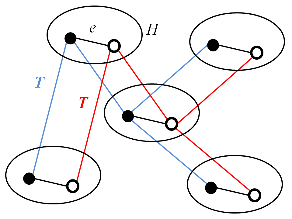
Figure 1: $T\mbox{ {\tiny$\!\!\square\,$}}K_{2}$ in $T\mbox{ {\tiny$\!\!\square\,$}}H$.

Definition.

For given graphs $T$ and $G$, let $\psi_{T}(G)$ be the graph with vertex set $\mathrm{Hom}(T,G)$ such that two vertices $h_{1},h_{2}\in\mathrm{Hom}(T,G)$ are adjacent if and only if $h_{1}(v)$ and $h_{2}(v)$ are adjacent in $G$ for all $v\in V(T)$.

The observation above essentially is equivalent to saying that a copy of $T\mbox{\raisebox{0.86108pt}{\tiny{$\,\square\,$}}}H$ in $G$ can be mapped to a copy of $H$ in $\psi_{T}(G)$, and the following lemma formalizes this intuition.

Lemma 3.1.

For all graphs $T$, $H$ and $G$, there exists a one-to-one correspondence between $\mathrm{Hom}(T\mbox{\raisebox{0.86108pt}{\tiny{$\,\square\,$}}}H,G)$ and $\mathrm{Hom}(H,\psi_{T}(G))$. In particular,

$$|\mathrm{Hom}(T\mbox{\raisebox{0.86108pt}{\tiny{$\,\square\,$}}}H,G)|=|\mathrm{Hom}(H,\psi_{T}(G))|.$$

Proof.

We will define $\xi:\mathrm{Hom}(T\mbox{\raisebox{0.86108pt}{\tiny{$\,\square\,$}}}H,G)\rightarrow\mathrm{Hom}(H,\psi_{T}(G))$ and $\varphi:\mathrm{Hom}(H,\psi_{T}(G))\rightarrow\mathrm{Hom}(T\mbox{\raisebox{0.86108pt}{\tiny{$\,\square\,$}}}H,G)$ such that $\xi\circ\varphi=id$.

For a given $h\in\mathrm{Hom}(T\mbox{\raisebox{0.86108pt}{\tiny{$\,\square\,$}}}H,G)$, for each $v\in V(H)$, define $h_{v}:V(T)\rightarrow V(G)$ as $h_{v}(w)=h(w,v)$ for each $w\in V(T)$. Whenever $w,w^{\prime}\in V(T)$ are adjacent, the vertices $h_{v}(w)=h(w,v)$ and $h_{v}(w^{\prime})=h(w^{\prime},v)$ are adjacent. Thus $h_{v}\in\mathrm{Hom}(T,G)$ for all $v\in V(H)$. Moreover, if $v,v^{\prime}$ are adjacent vertices of $H$, then $h_{v}(w)=h(w,v)$ and $h_{v^{\prime}}(w)=h(w,v^{\prime})$ are adjacent, and thus $h_{v}$ and $h_{v}^{\prime}$ are adjacent in $\psi_{T}(G)$. Hence if we let $\xi(h)\,:\,V(H)\rightarrow\mathrm{Hom}(T,G)$ be defined by $\xi(h)(v)=h_{v}$, then $\xi$ is a map from $\mathrm{Hom}(T\mbox{\raisebox{0.86108pt}{\tiny{$\,\square\,$}}}H,G)$ to $\mathrm{Hom}(H,\psi_{T}(G))$.

On the other hand, given a map $g\in\mathrm{Hom}(H,\psi_{T}(G))$, define $\varphi(g):V(T)\times V(H)\rightarrow V(G)$ as $\varphi(g)(w,v)=g(v)(w)$ for each $v\in V(H)$ and $w\in V(T)$. We first prove that $\varphi(g)\in\mathrm{Hom}(T\mbox{\raisebox{0.86108pt}{\tiny{$\,\square\,$}}}H,G)$. For edges of the form $\{(w,v),(w^{\prime},v)\}$, $\varphi(g)(w,v)=g(v)(w)$ and $\varphi(g)(w^{\prime},v)=g(v)(w^{\prime})$ are adjacent since $g(v)\in V(\psi_{T}(G))=\mathrm{Hom}(T,G)$. For edges of the form $\{(w,v),(w,v^{\prime})\}$, we have $\varphi(g)(w,v)=g(v)(w)$ and $\varphi(g)(w,v^{\prime})=g(v^{\prime})(w)$, and these two vertices are adjacent in $G$ since $g(v)$ and $g(w)$ are adjacent in $\psi_{T}(G)$. Hence we established that $\varphi(G)\in\mathrm{Hom}(T\mbox{\raisebox{0.86108pt}{\tiny{$\,\square\,$}}}H,G)$.

It suffices to prove the $\xi\circ\varphi=id$. This follows from the fact that for $h\in\mathrm{Hom}(T\mbox{\raisebox{0.86108pt}{\tiny{$\,\square\,$}}}H,G)$, $v\in V(H)$ and $w\in V(T)$,

$$\left((\varphi\circ\xi)(h)\right)(w,v)=h_{v}(w)=h(w,v),$$

for the map $h_{v}$ defined as above. ∎

By Lemma 3.1, we can now estimate the size of $\mathrm{Hom}(T\mbox{\raisebox{0.86108pt}{\tiny{$\,\square\,$}}}H,G)$ through estimating the size of $\mathrm{Hom}(H,\psi_{T}(G))$, where Sidorenko’s property of $H$ provides a lower bound on the size of $\mathrm{Hom}(H,\psi_{T}(G))$. We can use this idea to show the simplest case of Theorem 1.2, i.e., when $T=K_{2}$. Here we give a full proof of this simple case, as the result will be used in the proof of Theorem 1.2.

Theorem 3.2.

If $H$ is a bipartite graph having Sidorenko’s property, then $K_{2}\mbox{\raisebox{0.86108pt}{\tiny{$\,\square\,$}}}H$ has Sidorenko’s property.

Proof.

Let $G$ be a given graph and put $\psi(G)=\psi_{K_{2}}(G)$ for simplicity. By Lemma 3.1 and the fact that $H$ has Sidorenko’s property, we have

$$|\mathrm{Hom}(K_{2}\mbox{\raisebox{0.86108pt}{\tiny{$\,\square\,$}}}H,G)| =|\mathrm{Hom}(H,\psi(G))|$$

$$\geq|V(\psi(G))|^{|V(H)|}\left(\frac{|\mathrm{Hom}(K_{2},\psi(G))|}{|V(\psi(G))|^{2}}\right)^{|E(H)|}$$

$$=|V(\psi(G))|^{|V(H)|-2|E(H)|}|\mathrm{Hom}(K_{2},\psi(G))|^{|E(H)|}.$$ (3.1)

We have

$$|V(\psi(G))|=|\mathrm{Hom}(K_{2},G)|=|V(G)|^{2}t_{K_{2}}(G).$$

On the other hand, by Lemma 3.1 with $H=K_{2}$, we have

$$|\mathrm{Hom}(K_{2},\psi(G))|=|\mathrm{Hom}(K_{2}\mbox{\raisebox{0.86108pt}{\tiny{$\,\square\,$}}}K_{2},G)|,$$

where since $K_{2}\mbox{\raisebox{0.86108pt}{\tiny{$\,\square\,$}}}K_{2}$ is isomorphic to $C_{4}$, by Sidorenko’s property of $C_{4}$, we have

$$|\mathrm{Hom}(K_{2}\mbox{\raisebox{0.86108pt}{\tiny{$\,\square\,$}}}K_{2},G)|=|V(G)|^{4}t_{C_{4}}(G)\geq|V(G)|^{4}(t_{K_{2}}(G))^{4}.$$

Therefore in (3), we get

$$|\mathrm{Hom}(K_{2}\mbox{\raisebox{0.86108pt}{\tiny{$\,\square\,$}}}H,G)| \geq\Big{(}|V(G)|^{2}t_{k_{2}}(G)\Big{)}^{|V(H)|-2|E(H)|}\cdot\Big{(}|V(G)|t_{K_{2}}(G)\Big{)}^{4|E(H)|}$$

$$=|V(G)|^{2|V(H)|}t_{K_{2}}(G)^{|V(H)|+2|E(H)|}.$$

Since $|V(K_{2}\mbox{\raisebox{0.86108pt}{\tiny{$\,\square\,$}}}H)|=2|V(H)|$ and $|E(K_{2}\mbox{\raisebox{0.86108pt}{\tiny{$\,\square\,$}}}H)|=2|E(H)|+|V(H)|$, we deduce that $K_{2}\mbox{\raisebox{0.86108pt}{\tiny{$\,\square\,$}}}H$ has Sidorenko’s property. ∎

If one attempts to use the same idea as in the proof of Theorem 3.2 to prove Theorem 1.2 for general graphs $T$ other than $K_{2}$, then the inequality corresponding to (3) will be

$$|\mathrm{Hom}(T\mbox{\raisebox{0.86108pt}{\tiny{$\,\square\,$}}}H,G)|\geq|V(\psi_{T}(G))|^{|V(H)|-2|E(H)|}|\mathrm{Hom}(K_{2},\psi_{T}(G))|^{|E(H)|}.$$

Thus we need estimates on $|V(\psi_{T}(G))|=|\mathrm{Hom}(T,G)|$ and $|\mathrm{Hom}(K_{2},\psi_{T}(G))|=|\mathrm{Hom}(K_{2}\mbox{\raisebox{0.86108pt}{\tiny{$\,\square\,$}}}T,G)|$. If $T$ has Sidorenko’s property, then $K_{2}\mbox{\raisebox{0.86108pt}{\tiny{$\,\square\,$}}}T$ also has Sidorenko’s property by Theorem 3.2. Hence in this case we have lower bound estimates on both $|V(\psi_{T}(G))|$ and $|\mathrm{Hom}(K_{2},\psi_{T}(G))|$. Unfortunately, these bounds do not transfer to a lower bound on $|\mathrm{Hom}(T\mbox{\raisebox{0.86108pt}{\tiny{$\,\square\,$}}}H,G)|$, since such a lower bound requires an upper bound on $|V(\psi_{T}(G))|$ if $|V(H)|-2|E(H)|<0$.

We solve this problem when $T$ is a tree, through the following lemma asserting that it suffices to consider graphs $G$ with bounded maximum degree.

Lemma 3.3.

A bipartite graph $H$ has Sidorenko’s property if and only if for all graphs $G$ with maximum degree at most $\frac{4|E(G)|}{|V(G)|}$,

$$t_{H}(G)\geq t_{K_{2}}(G)^{|E(H)|}.$$

We also need the following lemma. We omit the proof, which is based on tensor products of graphs. One may refer to Remark 2 of [20] (English version) for more details.

Lemma 3.4.

Let $H$ be a bipartite graph. If there exists a constant $c$ depending only on $H$ such that

$$t_{H}(G)\geq c(t_{K_{2}}(G))^{|E(H)|}~{}~{}~{}\mbox{for all graphs $G$,}$$

then $H$ has Sidorenko’s property.

Proof of Lemma 3.3.

We may assume that $H$ has no isolated vertex, as adding an isolated vertex to a graph does not affect the value of $t_{H}(G)$ and $|E(H)|$.

Suppose that $H$ is a bipartite graph satisfying the given condition, and let $G$ be an arbitrary graph (not necessarily satisfying the maximum degree condition).

Let $\Delta=\frac{2|E(G)|}{|V(G)|}$, and let $G^{\prime}$ be a graph obtained from $G$ by the following process. Fix an ordering of the vertices of $G$, and take vertices $v$ one at a time according to the ordering. Replace $v$ with $t=\lceil\frac{\deg(v)}{\Delta}\rceil$ vertices $v_{1},\cdots,v_{t}$ and choose the neighbors of these new vertices so that (i) $N(v_{i})\subseteq N(v)$, (ii) $N(v_{i})\cap N(v_{j})=\emptyset$ for all distinct pairs $i,j$, and (iii) $\deg(v_{i})\leq\Delta$ for all $i$. Note that such a choice exists, as one can greedily assign the neighbors of $v$ to the vertices $v_{i}$ under the given constraints. Further note that during this process, $\deg(v)$ remains the same until $v$ is replaced, and the number of edges always remains the same as $|E(G)|$.

Define a function $\pi:V(G^{\prime})\rightarrow V(G)$ as $\pi(v_{i})=v$ for all $i$. Since $\pi$ is a homomorphism from $G^{\prime}$ to $G$, we obtain a map $\phi:\mathrm{Hom}(H,G^{\prime})\rightarrow\mathrm{Hom}(H,G)$ such that $\varphi(h):=\pi\circ h$. Further note that for an adjacent pair of vertices $v,w\in V(G)$, there exists a unique choice of $v^{\prime}\in\pi^{-1}(v)$ and $w^{\prime}\in\pi^{-1}(w)$ such that $v^{\prime}$ and $w^{\prime}$ are adjacent in $G^{\prime}$. Therefore if $\pi\circ h_{1}=\pi\circ h_{2}$ for some $h_{1},h_{2}\in\mathrm{Hom}(H,G^{\prime})$, then for each edge $\{x,y\}$ of $H$, we must have $h_{1}(x)=h_{2}(x)$ and $h_{1}(y)=h_{2}(y)$. Since $H$ has no isolated vertex, we see that $h_{1}(x)=h_{2}(x)$ for all $x\in V(H)$, i.e. $h_{1}=h_{2}$. This implies that our map $\varphi$ from $\mathrm{Hom}(H,G^{\prime})$ to $\mathrm{Hom}(H,G)$ is an injection. Therefore, $|\mathrm{Hom}(H,G)|\geq|\mathrm{Hom}(H,G^{\prime})|$.

The graph $G^{\prime}$ has the same number of edges as the graph $G$, and the number of vertices is at most

$$|V(G^{\prime})| =\sum_{v\in V(G)}\left\lceil\frac{\deg(v)}{\Delta}\right\rceil$$

$$\leq|V(G)|+\sum_{v\in V(G)}\frac{\deg(v)}{\Delta}=|V(G)|+\frac{2|E(G)|}{\Delta}=2|V(G)|.$$

Combining this with the fact $|E(G^{\prime})|=|E(G)|$, it follows that $G^{\prime}$ has maximum degree $\Delta=\frac{2|E(G)|}{|V(G)|}\leq\frac{4|E(G^{\prime})|}{|V(G^{\prime})|}$. Hence $G^{\prime}$ satisfies the given maximum degree condition, so

$$|\mathrm{Hom}(H,G)|\geq\, |\mathrm{Hom}(H,G^{\prime})|\geq|V(G^{\prime})|^{|V(H)|}\left(\frac{2|E(G^{\prime})|}{|V(G^{\prime})|^{2}}\right)^{|E(H)|}$$

$$\geq\, 2^{|V(H)|-2|E(H)|}|V(G)|^{|V(H)|}\left(\frac{2|E(G)|}{|V(G)|^{2}}\right)^{|E(H)|}.$$

By Lemma 3.4, this concludes the proof. ∎

We are now ready to prove Theorem 1.2. As mentioned above, the proof follows the same line as of the proof of Theorem 3.2, and uses Theorem 3.2 as an ingredient.

Proof of Theorem 1.2.

We may assume that $H$ has no isolated vertex, as adding an isolated vertex to a graph does not affect the value of $t_{H}(G)$ and $|E(H)|$.

Let $T$ be a tree with $\tau$ vertices, and let $G$ be a given graph. By Lemma 3.3, we may assume that $G$ has maximum degree at most $\frac{4|E(G)|}{|V(G)|}=2|V(G)|t_{K_{2}}(G)$. By Lemma 3.1 and the fact that $H$ has Sidorenko’s property, we have

$$|\mathrm{Hom}(T\mbox{\raisebox{0.86108pt}{\tiny{$\,\square\,$}}}H,G)| =|\mathrm{Hom}(H,\psi_{T}(G))|$$

$$\geq|V(\psi_{T}(G))|^{|V(H)|}\left(\frac{|\mathrm{Hom}(K_{2},\psi_{T}(G))|}{|V(\psi_{T}(G))|^{2}}\right)^{|E(H)|}$$

$$=|V(\psi_{T}(G))|^{|V(H)|-2|E(H)|}|\mathrm{Hom}(K_{2},\psi_{T}(G))|^{|E(H)|}.$$ (3.2)

Recall that $V(\psi_{T}(G))=\mathrm{Hom}(T,G)$. We can construct an element in $\mathrm{Hom}(T,G)$ by starting from an arbitrary vertex of $T$, defining its image in $V(G)$, and then extending the homomorphism one vertex at a time. By the condition on the maximum degree of $G$, we thus have

$$|V(\psi_{T}(G))| =|\mathrm{Hom}(T,G)|\leq|V(G)|\Big{(}2|V(G)|t_{K_{2}}(G)\Big{)}^{\tau-1}$$

$$=2^{\tau-1}|V(G)|^{\tau}t_{K_{2}}(G)^{\tau-1}.$$ (3.3)

On the other hand, by Lemma 3.1 with $H=K_{2}$ and Theorem 3.2, we have

$$|\mathrm{Hom}(K_{2},\psi_{T}(G))|=|\mathrm{Hom}(T\mbox{\raisebox{0.86108pt}{\tiny{$\,\square\,$}}}K_{2},G)|\geq|V(G)|^{2\tau}t_{K_{2}}(G)^{3\tau-2}.$$ (3.4)

Since $H$ has no isolated vertex, we have $|V(H)|\leq 2|E(H)|$, and thus in (3), we may use the bounds from (3.3) and (3.4) to obtain

$$|\mathrm{Hom}(T\mbox{\raisebox{0.86108pt}{\tiny{$\,\square\,$}}}H,G)|$$

$$\geq\, \Big{(}2^{\tau-1}|V(G)|^{\tau}t_{K_{2}}(G)^{\tau-1}\Big{)}^{|V(H)|-2|E(H)|}\Big{(}|V(G)|^{2\tau}t_{K_{2}}(G)^{3\tau-2}\Big{)}^{|E(H)|}$$

$$=\, 2^{(\tau-1)(|V(H)|-2|E(H)|)}\cdot|V(G)|^{\tau|V(H)|}t_{K_{2}}(G)^{(\tau-1)|V(H)|+\tau|E(H)|}.$$

Since $|V(T\mbox{\raisebox{0.86108pt}{\tiny{$\,\square\,$}}}H)|=\tau|V(H)|$ and $|E(T\mbox{\raisebox{0.86108pt}{\tiny{$\,\square\,$}}}H)|=(\tau-1)|V(H)|+\tau|E(H)|$, by Lemma 3.4, we deduce that $T\mbox{\raisebox{0.86108pt}{\tiny{$\,\square\,$}}}H$ has Sidorenko’s property. ∎

Since an arbitrary $d$-dimensional grid can be obtained from the Cartesian product of $d$ paths, we obtain the following corollary.

Corollary 3.5.

For all $d\geq 1$, all $d$-dimensional grids have Sidorenko’s property.

4 Concluding Remarks

In this section, we will say more about tree-arrangeability and possible extensions of Theorem 1.2. First, we will provide a simple description of tree-arrangeability in terms of the vertices with maximal neighbors. Second, we will explain how the tree-arrangeability is related to tree decompositions and Markov Random Field. We conclude by proposing a couple of open questions related to Cartesian products that may illuminate a way to attack Sidorenko’s conjecture.

Tree-arrangeability and vertices with maximal neighborhood. To see whether a bipartite graph $H$ with bipartition $A\cup B$ is tree-arrangeable, it suffices to consider only the vertices in $A$ whose neighborhoods are maximal with respect to inclusion. A subset $U$ of $A$ is called neighbor covering if for each $a\in A$, there exists $u\in U$ such that $\Lambda_{a}\subseteq\Lambda_{u}$. If a neighbor covering set $U$ is $T$-arrangeable for a tree $T$ on $U$, then the tree on $A$ obtained by adding each $a\in A\setminus U$ to $T$ as a leaf adjacent to $u\in U$ with $\Lambda_{a}\subseteq\Lambda_{u}$ (if more than one such $u$ exists, then choose arbitrary one among them) makes $A$ tree-arrangeable. Hence $H$ is tree-arrangeable if and only if there exists a neighbor covering set $U\subseteq A$ that is tree-arrangeable. The cases when there exists a neighbor covering set of size one or two were discussed in the introduction.

Tree-arrangeability and tree decompositions. Tree-arrangeability can be alternatively defined using tree decompositions. A tree decomposition of a graph $H$, introduced by Halin [9] and developed by Robertson and Seymour [18], is a pair $(\mathcal{F},T)$ of a family $\mathcal{F}$ of vertex subsets and a tree $T$ with vertex set $\mathcal{F}$ satisfying

1. $\bigcup_{X\in\mathcal{F}}X=V(H)$,

2. for each $\{v,w\}\in E(H)$, there exists a set $X\in\mathcal{F}$ such that $v,w\in X$, and

3. for $X,Y,Z\in\mathcal{F}$, $X\cap Y\subseteq Z$ whenever $Z$ lies on the path from $X$ to $Y$ in $T$.

It is straightforward to check that a bipartite graph $H$ with bipartition $A\cup B$ is tree-arrangeable if and only if there exists a tree decomposition of $H$ with $\mathcal{F}=\{\Lambda_{a}\cup\{a\}\,|\,a\in A\}$.

Markov Random Field. Tree-arrangeability and the functions $f_{u}$ defined in Section 2 are also closely related to Markov Random Field theory.

A sequence of random variables $(y_{v})_{v\in V(G)}$ is said to be a Markov Random Field with respect to a graph $G$ if for each $S\subseteq V(G)$ that makes $G\setminus S$ disconnected, whenever $C_{1}$ and $C_{2}$ are the vertex sets of distinct components of $G\setminus S$, the pair of sequences of random variables $(y_{v})_{v\in C_{1}}$ and $(y_{v})_{v\in C_{2}}$ is independent, conditioned on $(y_{v})_{v\in S}$. Lemma 2.3 (iii) shows that if a bipartite graph $H$ with bipartition $A\cup B$ is tree-arrangeable with a tree $T$ on $A$, then $(f_{v})_{v\in A}$ for the random variables $f_{v}$ defined in Section 2 is a Markov Random Field with respect to $T$. It would be interesting to further investigate the connection between the theory of Markov Random Fields and Sidorenko’s conjecture.

Extension of Cartesian product to non-bipartite graphs. For a given (not necessarily bipartite) graph $H$, define a bipartite graph $\phi(H)$ as follows: The bipartition of $\phi(H)$ consists of two disjoint copies of $V(H)$. Two vertices in distinct parts are adjacent in $\phi(H)$ if they are copies of the same vertex in $H$, or two adjacent vertices in $H$. In particular, $\phi(H)$ has $2|E(H)|+|V(H)|$ edges.

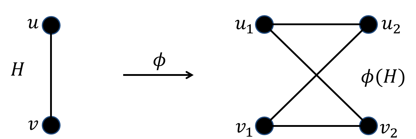
Figure 2: Blow-up via $\phi$.

It is not too difficult to see that for bipartite graphs $H$, we have $\phi(H)=K_{2}\mbox{\raisebox{0.86108pt}{\tiny{$\,\square\,$}}}H$. Hence the operation $\phi$ is more restricted than Cartesian products when considering bipartite graphs. However, the operation $\phi$ has the advantage of being applicable to non-bipartite graphs. For example, since $\phi(K_{k})=K_{k,k}$, we know that $\phi(K_{k})$ has Sidorenko’s property for all $k\geq 2$. Thus $\phi(H)$ may have Sidorenko’s property even if $H$ is a non-bipartite graph. Also note that $\phi(C_{5})$ is $K_{5,5}\setminus C_{10}$ which is the minimal bipartite graph unknown to satisfy Sidorenko’s conjecture. The operation $\phi$ provides many interesting graphs for which Sidorenko’s conjecture is not known to be true.

We conclude the paper with some open problems regarding the operator $\phi$. We believe that the family $\{\phi(C_{2k+1})\}_{k\geq 1}$ can be an interesting starting point in further studying Sidorenko’s conjecture. The only known graph to have Sidorenko’s property in this family is $C_{3}$.

Question 4.1.

Does there exist an integer $k\geq 2$ such that $\phi(C_{2k+1})$ has Sidorenko’s property?

Since $\phi(H)=K_{2}\mbox{\raisebox{0.86108pt}{\tiny{$\,\square\,$}}}H$ for bipartite graphs, Theorem 1.2 implies that $\phi(H)$ has Sidorenko’s property as long as $H$ does. Hence $\phi(H)$ is ‘more likely’ to have Sidorenko’s property than $H$. For example, since $\phi(K_{r})=K_{r,r}$ for integers $r\geq 1$, we know that $\phi(K_{r})$ has Sidorenko’s property, while $K_{r}$ is not even a bipartite graph. (Recall that a graph $H$ with odd cycles cannot satisfy Sidorenko’s property as $t_{H}(G)=0$ for bipartite graphs $G$). Thus, the following question may be posed.

Question 4.2.

For a (not necessarily bipartite) graph $H$, does there exist a non-negative integer $k=k_{{}_{\!H}}$ such that $\phi^{k}(H)$ has Sidorenko’s property?

If Sidorenko’s conjecture is true, then it certainly implies that the answers to the questions above are both yes. Even if Sidorenko’s conjecture turns out to be false, it is possible that the answers to the questions are positive.

Acknowledgement. Part of this work was done while Choongbum Lee and Joonkyung Lee were visiting Jeong Han Kim at KIAS. We would like to thank David Conlon for his useful comments and suggestion to consider the grid graphs, and Jacob Fox for providing the idea behind Lemma 3.3. We would also like to thank the anonymous referee for the valuable comments.

References

• [1] I. Benjamini and Y. Peres, A correlation inequality for tree-indexed Markov chains, in Seminar on Stochastic Processes, Proc. Semin., Los Angeles/CA (USA) 1991, Prog. Probab. 29, 1992, 7–14.
• [2] G. Blakley and P. Roy, Hölder type inequality for symmetrical matrices with non-negative entries, Proc. Amer. Math. Soc. (1965) 16, 1244-1245.
• [3] D. Conlon, J. Fox, and B. Sudakov, An approximate version of Sidorenko’s conjecture, Geom. Funct. Anal. 20 (2010), 1354-1366.
• [4] R. Daudel, R. Lefebvre, and C. Moser, Quantum chemistry: Methods and applications, Interscience Publishers, New York-London (1959).
• [5] P. Erdős and M. Simonovits, Cube-supersaturated graphs and related problems, in Progress in graph theory (Waterloo, Ont., 1982), Academic Press, Toronto, ON, 1984, 203-218.
• [6] P. Erdős and A. H. Stone, On the structure of linear graphs, in Bull. Amer. Math. Soc. 52(12) (1946), 1087-1091.
• [7] C. M. Fortuin, P.W. Kasteleyn, and J. Ginibre, Correlation inequalities on some partially ordered sets, Comm. Math. Phys. 22 (1971), 89-03.
• [8] Hans-Otto Georgii, Gibbs measures and phase transitions, Walter de Gruyter (1988).
• [9] R. Halin, S-functions for graphs, J. Geom. 8 (1976), 171-186.
• [10] H. Hatami, Graph norms and Sidorenko’s conjecture, Israel J. Math.175 (2010), 125-150.
• [11] D. London, Two inequalities in nonnegative symmetric matrices. Pac. J. Math. 16, 515-536 (1966)
• [12] L. Lovász and M. Simonovits, On the number of complete subgraphs in a graph II, Studies in pure mathematics, Birkhäuser (1983), 459-495.
• [13] H. Mulholland and C. Smith, An inequality arising in genetical theory, Amer. Math. Monthly (1959) 66, 673–683.
• [14] V. Nikiforov, The number of cliques in graphs of given order and size, Trans. Amer. Math. Soc. 363 (2011), 1599-1618.
• [15] R. Pemantle and Y. Peres, Domination between trees and application to an explosion problem, Ann. Probab. 22 (1994), 180-194
• [16] A. Razborov, On the minimal density of triangles in graphs, Combin. Probab. Comput. 17 (2008), 603-618.
• [17] C. Reiher, The clique density theorem, arXiv:1212.2454 [math.CO].
• [18] N. Robertson and P. D. Seymour, Graph minors III: Planar tree-width, J. Combin. Theory Ser. B. 36(1) (1984), 49-64.
• [19] A. F. Sidorenko, Extremal problems in graph theory and inequalities in functional analysis (in Russian), in Proceedings of the Soviet Seminar on Discrete Mathematics and its applications (in Russian), ed. Lupanov, O.B., Moscow, Moscow State University (1986), 99-105.
• [20] A. F. Sidorenko, Inequalities for functionals generated by bipartite graphs, Diskretnaya Matematika 3 (1991), 50-65 (in Russian), Discrete Math. Appl. 2 (1992), 489-504 (in English).
• [21] A. F. Sidorenko, A correlation inequality for bipartite graphs, Graphs Combin. 9 (1993), 201-204.
• [22] A. F. Sidorenko, An analytic approach to extremal problems for graphs and hypergraphs,in Extremal problems for finite sets (Visegrád, 1991), Bolyai Soc. Math. Stud., 3, János Bolyai Math. Soc., Budapest, 1994, 423-455.
• [23] M. Simonovits, Extremal graph problems, degenerate extremal problems and super-saturated graphs, in Progress in graph theory (Waterloo, Ont., 1982), Academic Press, Toronto, ON, 1984, 419-437.
• [24] Stan Z. Li. Markov Random Field Modeling in Image Analysis, Springer (2001).
• [25] G. Stell, Generating functionals and graphs, in Graph Theory and Theoretical Physics, Academic Press, London (1967), 281–300.
• [26] J.X. Li and B. Szegedy, On the logarithimic calculus and Sidorenko’s conjecture, arXiv:1107.1153 [math.CO].
• [27] P. Turán, Eine Extremalaufgabe aus der Graphentheorie, Mat. Fiz. Lapok 48 (1941), 436–452.