Alternating lags of QPO harmonics $:$ A Generic model and its application to the 67 millihertz QPO of GRS 1915+105

Abstract

A generic model for alternating lags in QPO harmonics is presented where variations in the photon spectrum are caused by oscillations in two parameters that characterize the spectrum. It is further assumed that variations in one of the parameters is linearly driven by variations in the other after a time delay $t_{d}$. It is shown that alternating lags will be observed for a range of $t_{d}$ values. A phenomenological model based on this generic one is developed which can explain the amplitude and phase lag variation with energy of the fundamental and the next three harmonics of the $67$ mHz QPO observed in GRS 1915+105. The phenomenological model also predicts the variation of the Bicoherence phase with energy, which can be checked by further analysis of the observational data.

1. INTRODUCTION

Quasi-periodic oscillations (QPO) have been observed in both black hole and neutron star systems. For black hole systems QPO have been observed for a wide range of frequencies from mHz to a few hundred Hz (McClintock & Remillard, 2006; Remillard & McClintock, 2006; van der Klis, 2006), while kHz QPO have also been observed in neutron star systems (van der Klis, 2000, 2006). The high frequency of these oscillations suggests that they probably originate in the innermost regions of these system and hence in principle could be used to probe and test effects of general relativity in the strong field limit. Since some of the low frequency QPO are observed to be correlated to the high frequency ones, they may have a common origin. Moreover, a study of the temporal behavior of these systems (particularly QPO activity) could give new insight into the enigmatic nature of these systems.

Theoretical studies of the QPO phenomena have generally been restricted to identifying the different frequencies as natural characteristic frequencies of the system and correlation between them (e.g. Miller et al., 1998; Stella & Vietri, 1999; Titarchuk & Osherovich, 1999). A consistent model incorporating radiative and dynamic mechanisms, that translates the natural frequency of the system to an observable QPO, remains illusive. Clues to such underlying processes can be obtained by studying the energy dependence of the QPO features like amplitude and phase lags (e.g. Cui, 1999; Lee et al., 2001; Li et al., 2013; Lin et al., 2000; Morgan et al., 1997; Qu et al., 2010; Reig et al., 2000; Rodriguez et al., 2002), especially when harmonics are observed since additional information can be obtained for the same phenomenon. Such an endeavor has been impeded, because the energy dependence of the phase lags for many QPO are observed to be complex and contrary to expectations (Cui et al., 2000; Remillard et al., 2002). For example, the soft photons are often observed to lag the high energy ones (Cui, 1999; Vaughan et al., 1998) which is contrary to simple Comptonization models, although recent studies have shown that under certain conditions a soft lag could arise when more than one physical parameter is oscillating (Lee et al., 2001). Further the time lags for low frequency QPO, $<1$ Hz, are often large, $>0.1$ s (Cui, 1999) and hence are probably not due to any radiative process and may be due to non-linear multiplicative reverberation effects (Shaposhnikov, 2012). Large time lags have also been observed for low frequency non periodic continuum fluctuations (Nowak et al., 1999) which are probably associated with the slow propagation of waves in an accretion disk (Nowak et al., 1999; Misra, 2000) or correspond to the rise/decay time of magnetic flares (Poutanen & Fabian, 1999).

Perhaps the most unexpected results are that for some QPO, the phase lag for the odd and even harmonics have opposite signs. Such alternating lag behavior have been observed at different frequencies, e.g. $67$ mHz (Cui, 1999) and $\approx 3$ Hz (Lin et al., 2000; Reig et al., 2000; Tomsick & Kaaret, 2001) for GRS 1915+105 and at $\approx 3$ Hz for XTE J1550-564 (Cui et al., 2000; Wijnands et al., 1999). Possible explanations for such phenomena include partial covering models (Varnière, 2005) or due to radiative transport of photons through a hot Comptonizing medium (Böttcher & Liang, 2000). Ingram et al. (2009) in their model proposed that QPO arises due to the Lense-Thirring precession of the hot inner flow. Based on this, Axelsson et al. (2013) explained the average spectrum and those of a QPO and its harmonic for XTE J1550-564, however it is not clear whether it can also explain the complex time-lag as function of energy. Axelsson et al. (2013) quote a recent work by Veledina et al. (2013) where they have shown that the existance of a strong harmonic is predicted by the angular radiation pattern from comptonisation of a precessing hot inner flow. Böttcher & Liang (2000) show that alternating lags for the $\approx 3$ Hz can be explained by time delays due to Comptonization but such a model is not applicable for the lower frequency QPO. Since alternating time lags for different harmonics have been observed for different frequencies and for different systems, any model for the phenomena has to be sufficiently generic and should not depend on the details of QPO production and/or radiative mechanism.

In this work, such a generic model is presented. It is shown that alternating lags will occur under fairly general conditions if the QPO is due to the oscillation of two dependent physical parameters. The two parameters could characterize a single component of the spectrum or could correspond to two different spectral components. Based on this interpretative framework, a phenomenological model is developed which can explain the complex energy dependent features of the $67$ mHz QPO observed in GRS 1915+105. In particular, the amplitude and phase lags with energy for the fundamental and the next three harmonics (a total of eight curves) is explained with this model consisting of six parameters. Predictions are made for the energy dependence of the phases of the Bicoherence function which, in principle, can be checked with further analysis of the observational data.

2. Generic model for alternating lags

Consider a photon spectrum $s(E)$, characterized by two physical parameters $a$ and $b$, such that the temporal variations in the spectrum $s(E,t)\rightarrow s_{o}(E)+\Delta s(E,t)$, are due to corresponding variations in $a(t)=a_{o}+\Delta a(t)$ and $b(t)=b_{o}+\Delta b(t)$. If the response of the spectrum to the variations in the parameters is linear, then

$$\Delta s(E,t)=\gamma_{a}(E)\Delta a(t)+\gamma_{b}(E)\Delta b(t)$$ (1)

where $\gamma_{a}$ and $\gamma_{b}$ are time independent functions of energy. In the above equation it has been assumed that the radiative process time-scale ( $\approx\tau L/c\approx 2$ msec, where $\tau\approx 1$ is the optical depth and $L\approx 50GM/c^{2}\approx 7\times 10^{7}cm$ is the size of the system for a ten solar mass black hole) is much shorter than the variability time-scale of the parameters. In other words, the time lag between the parameter variations and the spectral response is negligible.

In this scenario, the variations in the spectral parameters ($\Delta a(t)$ and $\Delta b(t)$) are caused by a driving dynamical oscillation which produces the QPO. It is further assumed that the variations in $b$ are also driven linearly by variations in $a$ after a time lag $t_{d}$, that is,

$$\Delta b(t)=F\Delta a(t-t_{d})+D(t)$$ (2)

where $F$ is a time independent constant and $D(t)$ denotes the direct coupling between the driving oscillation and $b$.

Although the direct coupling term ($D(t)$) may not be negligible compared to the interactive term ($F\Delta a(t-t_{d})$) for some systems ( e.g. section 3 below), it is convenient to neglect $D(t)$ at this stage, only to illustrate how such a model could produce alternating lags.With this assumption a simple equation for the phase lags can be written which explains the origin of the alternating lag behavior in a straight forward manner. Neglecting $D(t)$ and combining Eqn. (1) and (2) gives,

$$\Delta S(E,\omega)=\gamma_{a}(E)\Delta A(\omega)[1+\gamma_{r}(E)e^{-i\omega t_{d}}]$$ (3)

where, $S(E,\omega)$ and $A(\omega)$ are the Fourier transforms of $s(E,t)$ and $a(t)$ respectively, $\omega$ is the angular frequency and $\gamma_{r}(E)\equiv F\gamma_{b}(E)/\gamma_{a}(E)$. The cross-spectrum $C(\omega,E_{1},E_{2})$ for two energies $E_{1}$ and $E_{2}$, is defined as $\equiv\Delta S^{*}(E_{1},\omega)\Delta S(E_{2},\omega)$. Thus

$$C(\omega,E_{1},E_{2}) = \gamma_{a}(E_{1})\gamma_{a}(E_{2})|\Delta A(\omega)|^{2}\times$$ (4)

$$[1+\gamma_{r}(E_{1})e^{i\omega t_{d}}][1+\gamma_{r}(E_{2})e^{-i\omega t_{d}}]$$

The phase, $\phi(\omega,E_{1},E_{2})$, of the cross-spectrum divided by $\omega$ is generally identified as the time lag between the photons of energy $E_{1}$ and $E_{2}$. From the form of Eqn. 4, it can be seen that this phase can be written as,

$$\hbox{sin }\phi = \frac{Im[C]}{|C|}$$ (5)

$$= {(\gamma_{r}(E_{1})-\gamma_{r}(E_{2}))\hbox{sin}(m\omega_{o}t_{d})\over|1+\gamma_{r}(E_{1})e^{i\omega t_{d}}||1+\gamma_{r}(E_{2})e^{-i\omega t_{d}}|}$$

Here $\omega$ has been replaced by $m\omega_{o}$ where $\omega_{o}$ is the angular frequency of the fundamental oscillation (first harmonic) and different values of the integer $m$ correspond to the other harmonics of the system. Since the denominator of Eqn. 5 is always positive, the sign of the phase angle is determined by $(\gamma_{r}(E_{1})-\gamma_{r}(E_{2}))\hbox{sin}(m\omega_{o}t_{d})$. This implies that the system will exhibit alternating lag signs for $n$ harmonics, provided $t_{d}$ lies within the range

$$\pi(1-1/m)<\omega_{o}t_{d}<\pi(1+1/m)$$ (6)

where $m=n+1$. For example, for a system with four harmonics with alternating lags (like the 67 mHz QPO in GRS 1915+105), the time lag $t_{d}$ is restricted to lie between $3/8$ and $5/8$ of $1/f_{o}$ where $f_{o}$ is the fundamental frequency. Note that the phase $\phi$ depends on function $\gamma_{r}(E)$ (Eqn 5) and in general could be small even though $t_{d}$ is required to be $\approx 1/f_{o}$ to satisfy condition (6).

It is useful to enumerate the different conditions that need to exist in a system for this model to be applicable. The first condition is that there needs to be at least two parameters which characterize the spectrum. This is generally true for most radiative models invoked to explain hard X-ray spectra. For example, in the Comptonization model, the spectrum depends on the optical depth and temperature of the Comptonizing region. It should be noted that the spectral parameters $a$ and $b$ need not necessarily characterize the same spectral component. For example, $a$ could characterize a soft (black body like) component of the spectrum while $b$ could be related to the hard X-ray power-law which lags the intrinsic one after a time delay. The second condition is that two of the parameters should be related to each other (Eqn 2). Again it is probably true in general that variations in one parameter will induce variations in the other. The third condition is that $t_{d}$, the interaction time-scale between the two parameters, is of the same order as $1/f_{o}$, where $f_{o}$ is the QPO frequency. This would only be true for those phenomena where the QPO producing mechanism is similar to the one coupling the two parameters. For example, if the QPO is being produced by a dynamic process and the coupling between the two parameters is also of a dynamic nature, then it is expected that $t_{d}\approx 1/f_{o}\approx t_{dyn}$, where $t_{dyn}$ is the dynamic time-scale. Finally the fourth condition is the restriction on $t_{d}$ for the system to show alternating lags (Eqn 6). If the previous three conditions are satisfied for most of the systems, then this final criterion is expected to occur in a fraction of them. It should be emphasized that if there is an observation of alternating lags for a large number of harmonics of a QPO, then for this model to be applicable, $t_{d}$ would need to be “fine tuned” to satisfy Eqn 6. Thus such a observation would indicate that this model is at least not in general applicable. However, for alternating lags up to three or four harmonics, condition (6) is not overtly restrictive. When the direct coupling $D(t)$ is not negligible, the criterion for a system to exhibit alternating lags becomes more complex than Eqn. 6 and depends on the strength and form of the interaction. In such cases, as shown in the next section, a more detailed calculation of the phase lags is required.

3. Application to 67 millihertz QPO of GRS 1915+105

A 67 mHz QPO with the next three harmonics with alternating lags was detected by RXTE during 1996 May 5 observation of the black hole system GRS 1915+105 (Morgan et al., 1997; Cui, 1999). Since the Q factor for this QPO is large (FWHM $\approx$ mHz for the fundamental), the underlying continuum is not expected to effect the phase lag results. This and the fact that a total of four harmonics were observed for this source makes this phenomenon an excellent candidate to test the generic model developed in the earlier section. To compare the observed values with ones predicted from the model, specific form and strength of the interactions between the driving oscillation and the spectral parameters have to be chosen. Here, such a specific set of interactions is presented which can explain the observed energy dependent trends of the QPO phase lag and amplitude.

Variations in the photon spectrum $s(E,t)$ are assumed to be linearly driven by variations in two parameters $a$ and $b$ (Eqn 1), such that

$${\Delta s(E,t)\over s_{o}(E)}=-E\Delta a(t)-\hbox{log}(E/E_{p})\Delta b(t)$$ (7)

where $s_{o}(E)$ is the time independent part of the spectrum The first term of the R.H.S is the linear response of the spectrum to perturbation in $a$ if $s(E)\propto e^{-Ea}$, while the second term is for the case when $s(E)\propto E^{-b}$. Thus Eqn (7) corresponds to the situation when the spectrum can be described as an exponentially cut-off power-law ( $s(E)\propto E^{-b}e^{-Ea}$) with $a$ characterizing the inverse of the cutoff energy and $b$ the power-law slope. In this interpretation, $E{{}_{p}}$ is the pivot energy over which power-law component varies. This is partly motivated by observations of the high energy ($E>3keV$) time averaged spectra of some black hole systems which can be approximately described as an exponentially cut-off power law. The time averaged spectrum for the observation showing the 67 mHz QPO, can be roughly (at 2% level) described as a exponentially cut-off power-law of index $\sim 1.8$ and cutoff energy $\sim 5$ keV. However, in general detailed spectral analysis of GRS 1915+105 have shown that its spectrum is generally more complex (e.g. Yadav et al., 1999; Zdziarski et al., 2001; Rodriguez et al., 2008) To avoid such complexities and to keep the temporal model presented here independent of specific spectral models, Eqn (7) is used here in this analysis with the caveat that in reality the response functions could be significantly more complex. The motivation here is to show that the generic model developed in section 2, is applicable to the 67 mHz QPO and there exists a simple set of equations which can explain the complex behavior of this phenomenon.

Since harmonics are observed in this system, at least one of the parameters should couple non-linearly to the unknown driving mechanism that produces the QPO. Further, since exactly four harmonics were observed, this suggests that the coupling is of a quartic nature. Hence it is assumed here that,

$$\Delta a(t)=R_{a}(1+\beta\hbox{cos}(\omega_{o}t))^{4}$$ (8)

where $1+\beta\hbox{cos}(\omega_{o}t)$ is the oscillating driver and $R_{a}$ is the coupling constant between it and $a$. These variations in $a$ cause variations in $b$ (Eqn 2) with a time delay $t_{d}$,

$$\Delta b(t)=F\Delta a(t-t_{d})+R_{b}\beta\hbox{cos}(\omega_{o}t)$$ (9)

Here it is assumed that the direct coupling between the driving oscillation and $b$ ($D(t)$) is linear and in phase with interaction causing $\Delta a(t)$. Eqn (7), (8) and (9) can now be solved to obtain the fractional rms amplitude and the phase lag as a function of energy for the fundamental and the next three harmonics. A detailed fitting to the observed data points would require convoluting the predicted time varying spectrum with the instrumental response function and binning the resultant folded spectrum in appropriate energy bins. However, since the motivation here is to show that qualitative trends in the data can be explained by the model, the theoretical variations are directly compared with the data points. The results are shown in figures 1 and 2. The six parameters required for the fit are $E_{p}$,$R_{a}$, $\beta$,$F$,$t_{d}$ and $R_{b}$. The phase lag as a function of energy for the three harmonics other than fundamental (figure 2) depends only on three of these parameters, $E_{p}$,$F$ and $t_{d}$. The variation of the fractional amplitude with energy of the same harmonics depends on two additional parameters $R_{a}$ and $\beta$, while the amplitude and phase lag of the fundamental with energy also depends on $R_{b}$.

It is encouraging to find that the observed relative amplitude of the different harmonics (including the observation that the amplitude of the fourth harmonic is larger than the third ) can be explained by a simple non-linear equation (8). In particular the Fourier transform of Eqn (8) leads to

$${\Delta A(\omega)\over R_{a}} = (2\beta+{3\over 2}\beta^{3})\delta(\omega-\omega_{o})+({3\over 2}\beta^{2}+{1\over 4}\beta^{4})\delta(\omega-2\omega_{o})$$ (10)

$$+({1\over 2}\beta^{3})\delta(\omega-3\omega_{o})+({1\over 16}\beta^{4})\delta(\omega-4\omega_{o})$$

which when combined with Eqn (7) and (9) sets the relative amplitude of the different harmonics (figure 1). However the interactions chosen here (Eqn. 8, 9) may not be unique and it may be possible that there exists more complex non-linear relationships which also give similar results. For example, $a(t)$ could be coupling non-linearly to $b(t)$ instead of the driver i.e. $a(t)=f_{nl}(b(t))$ , where $f_{nl}$ is a nonlinear function. However, such a function would give different phase lags between the harmonics than those computed using Eqn (8). The phase lag between the harmonics can be indirectly measured using the phases of the Bicoherence function which is defined as (Maccarone & Coppi (2002); Maccarone et al. (2011); Maccarone (2013))

$$B_{nm}(E)\equiv\Delta S_{n}(E)\Delta S_{m}(E)\Delta S_{m+n}^{*}(E)$$ (11)

where the integer sub script on $\Delta S(E)$ stands for different harmonics. Figure 3 shows the predicted values of the phase of $B_{11}$, $B_{12}$ and $B_{22}$ as a function of energy using Eqn (7), (8) and (9). These variations can be directly compared with the observed values to test the validity of these equations and confirm the model developed here. Significant differences from the predicted values would perhaps indicate that the non-linear equation (8) is more complex than the one assumed in this work.

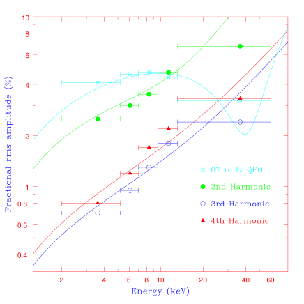
Figure 1.— Variation of the fractional rms amplitude with energy for the 67 mHz QPO and the next three harmonics. Data points are from Cui (1999) and with errors (not shown) smaller than $0.2$ %. Solid lines are model predictions (from top to bottom: fundamental (1st harmonic), 2nd harmonic, 4th harmonic and 3rd harmonic). The six parameters used in this fit are $E_{p}=0.5$ keV, $R_{a}=2.3\times 10^{-6}$ keV^-1, $\beta=9$, $F=-4$ keV, $\omega_{o}t_{d}=1.15\pi$ and $R_{b}=-7.2\times 10^{-3}$.

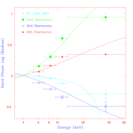
Figure 2.— Variation of the hard phase lag with energy for the 67 mHz QPO and next three harmonics. Data points are from Cui (1999). Points without error bars have error smaller than the symbols. Solid lines are model predictions (from top to bottom: 2nd harmonic, 4th harmonic, fundamental (1st harmonic) and 3rd harmonic). The parameters used for the model are same as in figure 1.

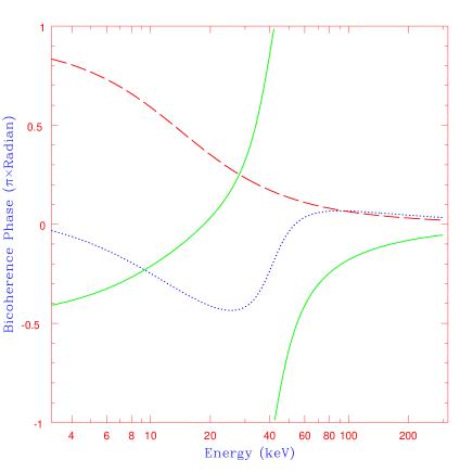
Figure 3.— Predicted variation of the phase of the Bicoherence function with energy. The parameters for the model are same as in figure 1. Solid line: phase of $B_{11}$ ; Dotted line: phase of $B_{12}$ ; Dashed line: phase of $B_{22}$.

4. Summary and discussion

The phenomenological model presented here should be developed further to incorporate the specific radiative and dynamic mechanism that could be operating for this system. The inferred weak coupling between the parameters($a$ and $b$) and the driving oscillation ($R_{a}=2.3\times 10^{-6}$ keV^-1 and $R_{b}=-7.2\times 10^{-3}$), could occur if the driving oscillation is localized to some particular radius of the accretion disk and hence couples weakly with the parameters which are probably global averages. A localized driver would also naturally explain why the QPO is so narrow ( FWHM $\approx$ mHz) since then the frequency could be associated with some natural frequency of the disk at that particular radius. However, it would then be difficult to understand why the time scale of interaction between the two (global) parameters $t_{d}$ is similar in magnitude to the timescale of the oscillation ($1/f$). If the form of the equation (8) is correct that would indicate that the physical quantity associated with the driver can have negative values since $\beta=9>1$. This means that the driving oscillation is not a positive physical quantity like temperature, density etc but needs to be associated with a quantity which can have negative values e.g. accretion rate, viscous stress etc.

In summary, a generic model for alternating lags for the harmonics of QPO has been presented. Based on the generic model, a phenomenological one has been developed to explain the amplitude and phase lag variation with energy of the harmonics of the 67 mHz QPO observed in GRS 1915+105. The model can be further strengthened and/or modified by comparing the predicted values of the phase of the Bi-coherence function with the ones inferred from observations. The model also puts restrictions on the radiative and dynamic mechanisms that are operating to produce this phenomenon. Physical models developed in the framework of the phenomenological one will enhance our understanding of these systems.

5. Acknowledgements

The research leading to these results has been partially funded by ISRO-RESPOND program. SM gratefully acknowledges IUCAA for the visiting associateship.

References

- Axelsson et al. (2013) Axelsson, M., Done, C., & Hjalmarsdotter,L. 2013, arXiv:1307.4396
- Böttcher & Liang (2000) Böttcher, M., & Liang, E.P. 2000, arXiv:astro-ph/0003139
- Cui (1999) Cui, W. 1999, ApJ, 524, L59
- Cui et al. (2000) Cui, W., Zhang, S. N., & Chen, W. 2000, ApJ, 531, L45
- Ingram et al. (2009) Ingram, A., Done, C., & Fragile, P. C. 2009, MNRAS, 397, L101
- Lee et al. (2001) Lee, H. C., Misra, R., & Taam, R. E. 2001, ApJ, 549, L229
- Li et al. (2013) Li, Z. B., Qu, J. L., Song, L. M., Ding, G. Q., & Zhang, C. M. 2013, MNRAS, 428, 1704
- Lin et al. (2000) Lin, D., Smith, I. A., Liang, E. P., & Böttcher, M. 2000, ApJ, 543, L141
- Maccarone & Coppi (2002) Maccarone, T. J., & Coppi, P. S. 2002, MNRAS, 336, 817
- Maccarone et al. (2011) Maccarone, T. J.,Uttley, P., van der Klis, M., Wijnands, R. A. D., & Coppi, P. S. 2011, MNRAS, 413, 1819
- Maccarone (2013) Maccarone, T. J. 2013, MNRAS, 2181
- McClintock & Remillard (2006) McClintock J. E. & Remillard R. A., 2006 , Compact Stellar X-ray Sources , Cambridge University Press, p.157
- Miller et al. (1998) Miller, M. C., Lamb, F. K., & Psaltis, D. 1998, ApJ, 508, 791
- Misra (2000) Misra, R. 2000, ApJ, 529, L95
- Morgan et al. (1997) Morgan, E. H., Remillard, R. A., & Greiner, J. 1997, ApJ, 482, 993
- Nowak et al. (1999) Nowak, M. A., Vaughan, B. A., Wilms, J., Dove, J. B., & Begelman, M. C. 1999, ApJ, 510, 874
- Poutanen & Fabian (1999) Poutanen, J., & Fabian, A. C. 1999, MNRAS, 306, L31
- Qu et al. (2010) Qu, J. L., Lu, F. J., Lu, Y., et al. 2010, ApJ, 710, 836
- Reig et al. (2000) Reig, P., Belloni, T., van der Klis, M., et al. 2000, ApJ, 541, 883
- Remillard et al. (2002) Remillard, R. A., Sobczak, G. J., Muno, M. P., & McClintock, J. E. 2002, ApJ, 564, 962
- Remillard & McClintock (2006) Remillard, R. A., & McClintock, J. E. 2006, ARA&A, 44, 49
- Rodriguez et al. (2002) Rodriguez, J., Durouchoux, P., Mirabel, I. F., et al. 2002, A&A, 386, 271
- Rodriguez et al. (2008) Rodriguez, J., Shaw, S. E., Hannikainen, D. C., Belloni, T., Corbel, S., Cadolle Bel, M., Chenevez, J., Prat, L., et al., 2008, ApJ, 675, 1449
- Shaposhnikov (2012) Shaposhnikov, N. 2012, ApJ, 752, L25
- Stella & Vietri (1999) Stella, L., & Vietri, M. 1999, Physical Review Letters, 82, 17
- Titarchuk & Osherovich (1999) Titarchuk, L., & Osherovich, V. 1999, ApJ, 518, L95
- Tomsick & Kaaret (2001) Tomsick, J. A., & Kaaret, P. 2001, ApJ, 548, 401
- Varnière (2005) Varnière, P. 2005, A&A, 434, L5
- van der Klis (2000) van der Klis, M. 2000, ARA&A, 38, 717
- van der Klis (2006) van der Klis, M. 2006, Compact Stellar X-ray Sources , Cambridge University Press, p.39
- Vaughan et al. (1998) Vaughan, B. A., van der Klis, M., Méndez, M., et al. 1998, ApJ, 509, L145
- Veledina et al. (2013) Veledina, A., Poutanen, J., & Ingram, A. 2013, MNRAS submitted.
- Wijnands et al. (1999) Wijnands, R., Homan, J., & van der Klis, M. 1999, ApJ, 526, L33
- Yadav et al. (1999) Yadav, J. S., Rao, A. R., Agrawal, P. C., Paul, B., Seetha, S. & Kasturirangan, K. 1999, ApJ, 517, 935
- Zdziarski et al. (2001) Zdziarski, A. A., Grove, J. E., Poutanen, J., Rao, A. R., & Vadawale, S. V. 2001, ApJ, 554, L45