SUPER-RESOLUTION IMAGING WITH AN ELT: KERNEL-PHASE INTERFEROMETRY

Abstract

Kernel-phase is a recently developed paradigm that tackles the classical problem of image deconvolution, based on an interferometric point of view of image formation. Kernel-phase inherits and borrows from the notion of closure-phase, especially as it is used in the context of non-redundant Fizeau interferometry, but extends its application to pupils of arbitrary shape, for diffraction limited images. The additional calibration brought by kernel-phase boosts the resolution of conventional images and enables the detection of otherwise hidden faint features at the resolution limit and beyond, a regime often refered to as super-resolution, which for a 30-meter telescope in the near IR, this translates into a resolving power smaller than 10 mas. Kernel-phase analysis of archival space and ground based AO data leads to new discoveries and/or improved relative astrometry and photometry. The paper presents the current status of the technique and some of its recent developments and applications that lead to recommendations for super-resolution imaging with ELTs.

1 Introduction

Imaging is the starting point of a lot of astronomical investigation: the image is the place where observers identify new sources, track their position relative to other reference points and/or follow their evolution as a function of time and/or wavelength. The image is indeed a remarkable locus in optics, where the photons of multiple sources are optimally segregated. Within the isoplanetic field of the instrument used for the acquisition, this image can be described as the result of the following convolution product:

$$I=O\otimes\mathrm{PSF},$$ (1)

where $I$, the distribution of intensity measured in the image, is a representation of the true structure of the object $O$, modified by the optical system point spread function $\mathrm{PSF}$. Imaging in the high-angular resolution regime essentially comes down to attempting to solve this deconvolution problem, and separate the two terms $I$ and $\mathrm{PSF}$. The problem is unfortunately ill-posed, with too many unknown for too few constraints. Adaptive optics (AO) obviously plays an important part in optimizing this segregation of photons, by concentrating the light of each source otherwise scattered over a large halo, into a narrow diffraction-limited pattern, that facilitates their identification.

Yet even at the highest Strehl, this apparently optimal segregation of photons is often not sufficient in solving some important problems such as: (1) the identification of faint sources or structures in the direct neighborhood of a bright object: in this context, the faint source one tries to detect is competing for the observer’s attention with the diffraction features of its host or (2) the discrimination of sources of comparable brightness so close to each other that they are said non-resolved.

Even if they are small, residual time-variable aberrations are responsible for the presence of a combination of static, quasi-static and rapidly evolving speckles in the image. Different schemes have been developed to sort out the PSF from the object function, and a fairly successful approach is to use some form of diversity in the PSF: angular differential imaging [10] for instance, uses field-rotation to differentiate true companions from quasi-static speckles. If enough field-rotation occurs over a time that is less than the characteristic quasi-static aberration time-scale, the diversity between the orientation of the sky and the quasi-static PSF allows the calibration of the PSF, leading to greatly enhanced detection limits. The calibration requires that the angular rotation induces sufficient local linear displacement of the genuine object features in order to avoid self-subtraction, which makes the technique little relevant for angular separations smaller than 0.5”. At small angular resolution, active alternatives are becoming available, with updated AO systems employing additional active optics to introduce wavefront diversity, to create higher-contrast regions in the image using techniques such as speckle nulling [13].

This paper presents an alternative approach, that looks at image formation from an interferometric point of view. Instead of focusing on the image, one examines its Fourier-transform counterpart. The approach builds upon the recent adaptation of non-redundant aperture masking interferometry to AO corrected images [16]. Non-redundant masking interferometry takes advantage of the self-calibration properties of an observable quantity called the closure-phase [9]. Closure-phase extracted from images acquired with a sparse aperture mask are indeed immune to residual wavefront of low spatial frequency, characterized by scale larger than the size of the sub-apertures, making them a powerful observable for high contrast imaging [6].

It was demonstrated that under high-Strehl conditions, the notion of closure-phase, requiring non-redundant aperture, can be generalized to arbitrarily shaped (i.e. including redundant) pupils [11]. Instead of trying to solve the ill-posed problem of image deconvolution posed in Eq. 1, the approach presented here allows to extract from conventional images observable quantities called kernel-phases that just like closure-phase, are immune to residual wavefront aberrations, including non-common path errors.

Section 2 introduces some simple examples that describe how one can generalize the original idea of closure-phase to make it compatible with redundant arrays. Section 3 explains how new observables called kernel-phases can be extracted from conventional well corrected images and Section 4 presents some applications.

2 Beyond the closure-phase in simple cases

Although the final application of this work is relevant to classical imaging with a conventional (i.e. non-sparse) telescope aperture, it is useful to go look at several sparse geometries to understand the basis for the model used for kernel-phase. In that scope, Fig. 1 features three of the simplest possible sparse pupil geometries, for which we examine the way the wavefront aberrations propage into the Fourier-transform of images. Although apertures are represented here with a non-negligible diameter for readability, in practice, they are considered to be point-like. For all geometries, Fig. 1 labels apertures with letters and baselines with couple of letters.

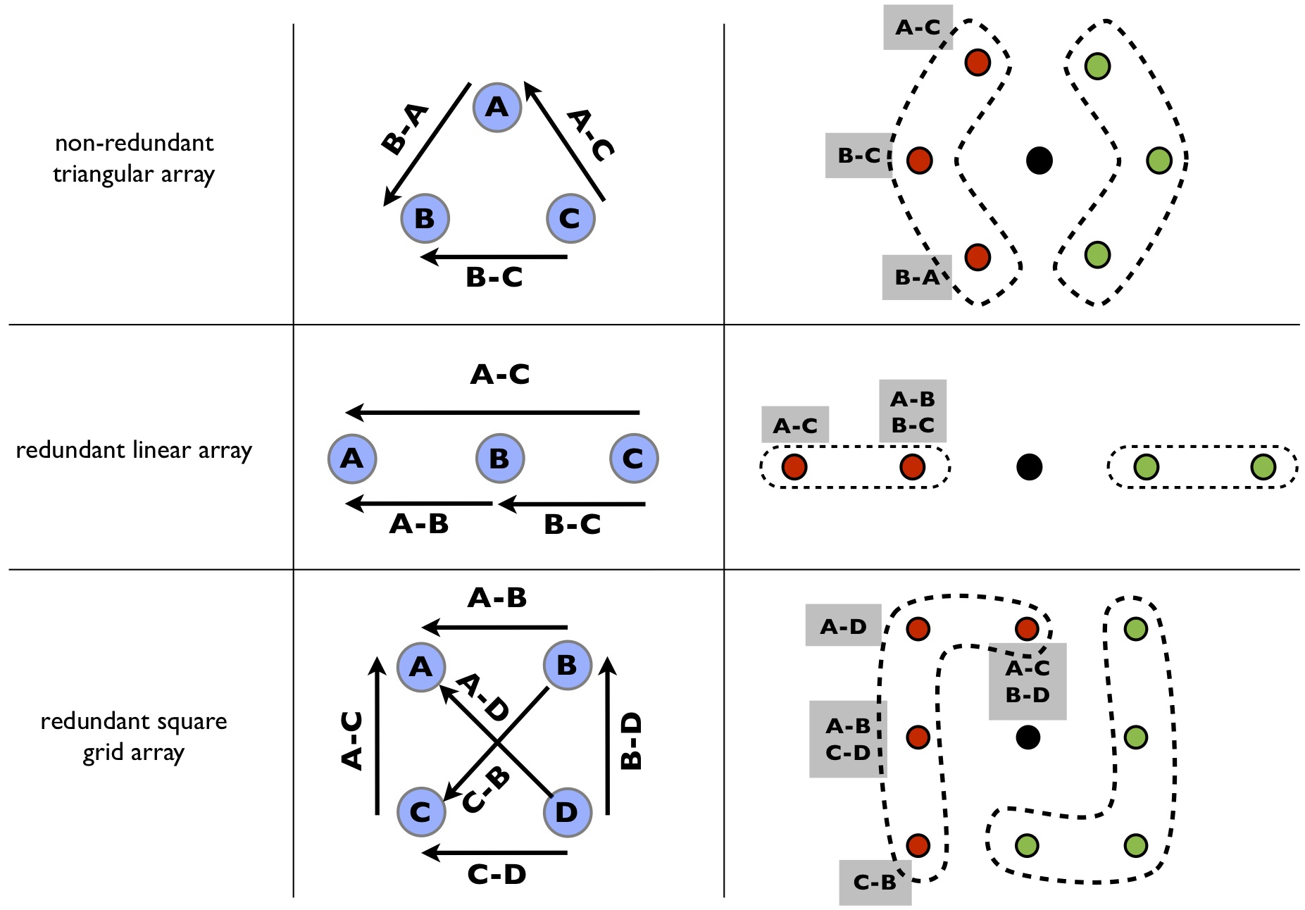
Figure 1: Pupil and corresponding $(u,v)$-coverage for three of the simplest possible sparse pupil geometries. From top to bottom: (1) non-redundant triangular array; (2) redundant linear array and (3) redundant square grid.

The first geometry, is a non-redundant 3-aperture array. Apertures are labeled $\mathrm{A}$, $\mathrm{B}$ and $\mathrm{C}$, and form three distinct baselines $\mathrm{A-C}$, $\mathrm{B-C}$ and $\mathrm{B-A}$. An image being a real function, its Fourier-transform exhibits some standard parity properties: it is even in amplitude and odd in phase, explaining why each baseline translates into a pair of points in the $(u,v)$-plane: only one of point per baseline needs to be considered: they are highlighted in red while their symmetric is in green. This work is for now restricted to the phase, and will ignore amplitude effects entirely. Each baseline gives access to a distinct measurement of the phase of the target of interest, a 3-component vector noted $\Phi_{O}$. This phase is however polluted by the phase delay along the baseline formed by the two apertures. The three equations for the different baselines phase simply write as:

$$\Phi^{BC} = \Phi_{O}^{BC}+(\varphi_{B}-\varphi_{C})$$

$$\Phi^{AC} = \Phi_{O}^{AC}+(\varphi_{A}-\varphi_{C})$$

$$\Phi^{BA} = \Phi_{O}^{BA}+(\varphi_{B}-\varphi_{A}).$$

It doesn’t take much to group these three equations into a compact matrix form:

$$\Phi = \Phi_{O}+\mathbf{A}\cdot\varphi,$$

$$\mathbf{A} = \begin{pmatrix}0&1&-1\\ 1&0&-1\\ -1&1&0\end{pmatrix}$$

with $\mathbf{A}$, referred to as the phase transfer matrix, encoding the information about the array. This geometry is often used to introduce the idea of closure-phase [14] in long-baseline interferometry. The sum of the phases measured along baselines forming a closing triangle: $\mathrm{C-B}$, $\mathrm{B-A}$, $\mathrm{A-C}$, is immune to the phase delay term $\varphi$. One can write this closure-phase relation in terms of a left-hand operator $\mathbf{K}=\begin{pmatrix}-1&1&1\end{pmatrix}$, that verifies $\mathbf{K}\cdot\mathbf{A}=\mathbf{0}$.

The second scenario presented in Fig. 1 is not as straightforrward, since one of the apertures of the previous array was moved so as to form a redundant baseline: $\mathrm{A-B}$ and $\mathrm{B-C}$ are indeed identical, while the baseline $\mathrm{A-C}$ remains unique. In the $(u,v)$-plane, the contributions of redundant baselines add up in the same place, resulting in two Fourier-phase components instead of three. Two baselines measure the same target phase object component $\Phi_{O}$, however each shifted by an amount that depends on the baseline phase delay. The resulting phase in this point is the argument of the sum of two phasors:

$$\Phi=\mathrm{Arg}[\exp{i(\Phi_{O}+\varphi_{A}-\varphi_{B})}+\exp{i(\Phi_{O}+\varphi_{B}-\varphi_{C})}].$$ (2)

For large phase delays (i.e. wavefront aberrations), this resulting phase can take any value between 0 and 2$\pi$. However if one assumes that phase errors are small ($\Delta\varphi\lesssim 1$ radian), which corresponds to a reasonable requirement on the AO system, Eq. 2 can be linearized and considerably simplifies as:

$$\Phi=\Phi_{O}+\frac{1}{2}(\varphi_{A}-\varphi_{C}).$$

Just like for the triangular geometry, the linear equations for the phase can be gathered into a compact matrix form:

$$\Phi=\Phi_{O}+\mathbf{R}^{-1}\cdot\mathbf{A}\cdot\varphi,$$ (3)

with:

$$\mathbf{R}^{-1}=\begin{pmatrix}1&0\\ 1&\frac{1}{2}\end{pmatrix}\mathrm{~{}~{}and~{}~{}}\mathbf{A}=\begin{pmatrix}1&0&-1\\ 1&0&-1\end{pmatrix}.$$

For this array, the only possible closure relation is $\mathbf{K}=\begin{pmatrix}1&-2\end{pmatrix}$. Here, the phase transfer matrix has been split into two components $\mathbf{R}^{-1}$ and $\mathbf{A}$, that respectively encode the redundancy of the baselines and the phase relationships.

With the last two examples in mind, and assuming that the linearization of Eq. 2 holds for arbitrarily redundant arrays, the last example is not difficult to write down directly using the same Eq. 3, with the following matrices:

$$\mathbf{R}^{-1}=\begin{pmatrix}1&0&0&0\\ 0&\frac{1}{2}&0&0\\ 0&0&1&0\\ 0&0&0&\frac{1}{2}\end{pmatrix}\mathrm{~{}~{}~{}and~{}~{}~{}}\mathbf{A}=\begin{pmatrix}1&0&0&-1\\ 1&-1&1&-1\\ 0&-1&1&0\\ 1&1&-1&-1\end{pmatrix}.$$

Two simple closure relations can be found by hand, and can again be summarized by a left-hand operator $\mathbf{K}$, so that:

$$\mathbf{K}=\begin{pmatrix}1&-2&1&0\\ 1&0&-1&-2\end{pmatrix}.$$

3 Kernel-phase

The three examples introduced in Section 2 suggest that, in the low-aberration (high-Strehl) regime, it is possible to identify, in the Fourier-phase space, a linear equivalent to the image-object convolution relation of eq. 1, of the form shown in eq. 3, even when the aperture is redundant. The most important element of this model is the phase transfer matrix $\mathbf{A}$, describing the way the pupil wavefront aberrations propagate into spurious phase in the Fourier-plane. The diagonal matrix $\mathbf{R}^{-1}$ is a scaling operator, that contains the inverse value of the baseline redundancy. $\mathbf{A}$ and $\mathbf{R}^{-1}$ can of course be combined into a single operator.

To work on data acquired with a conventional telescope aperture, one must start by building a discrete model of the pupil. Figure 2 shows one working example for the “medium cross pupil” of the Palomar Hale Telescope PHARO instrument [2]. The discrete model of the instrument pupil, uses a regular grid pattern, whose density is representative of the continuous pupil.

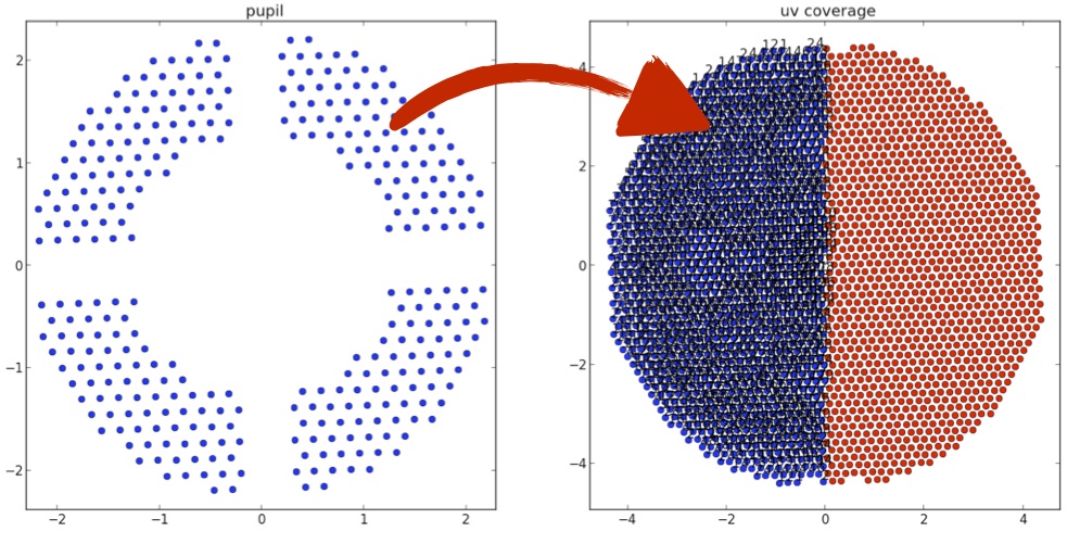
Figure 2: Example of discrete model that allows to construct the operator $\mathbf{A}$ that describes the way the pupil phase $\varphi$ propagates into the Fourier-plane (cf. Eq. 3). Left: discrete model of the pupil of the instrument, following a regular hexagonal grid. Right: the resulting distribution of spatial frequencies sampled by this geometry.

The model in Fig. 2 projects 332 pupil elements onto a grid of 1128 distinct sample points in the Fourier domain. The system is obviously large enough to justify delegating the identification of the kernel-phase operator $\mathbf{K}$ to an automated algorithm. One possible solution can be found as one of the products of the singular value decomposition (SVD) or the phase transfer matrix $\mathbf{A}$. The total number of kernel-phase relations $n_{K}$ is given by the number of zero singular values of $\mathbf{A}$. If the SVD of $\mathbf{A}$ writes as: $\mathbf{A}=\mathbf{U}\mathbf{W}\mathbf{V}^{T}$, where $\mathbf{W}$ is a diagonal matrix containing the singular values of $\mathbf{A}$, and $\mathbf{U}$ and $\mathbf{V}^{T}$ are unitary matrices, one possible set of orthogonal kernel-phase relations can be found in the columns of $\mathbf{U}$ that correspond to zeros on the diagonal of $\mathbf{W}$. They form an orthonormal basis for the left null space (or kernel) of the phase transfer matrix, hence the name kernel-phase.

Gathered into the operator $\mathbf{K}$, these relations are then applied to the phase measured in the Fourier plane $\Phi$, to extract information about the target of interest that is immune to residual wavefront error $\varphi$:

$$\mathbf{K}\cdot\Phi=\mathbf{K}\cdot\Phi_{O}.$$ (4)

Just like with closure phase, that collapses several phase measurements into a reduced number of observable quantities, some of the phase information seems lost in the process: these high quality can however be used as constraints for an interferometric imaging algorithm, or a parametric model. The SVD of the phase transfer matrix for the model shown in Fig. 2 shows that 962 kernel-phases can be extracted from any single image, which means that 85 % of the phase information is directly recoverable.

Once the paving of the $(u,v)$-plane and the matching kernel-phase relations are identified, they are saved in a template and used for extracting the phase information from the data. Before being Fourier-transformed, frames undergo traditional dark subtraction and flat-fielding procedure. To limit the impact of detector readout noise, the data can can be windowed, for instance with a “super-Gaussian” ($\exp{-(r/r_{0})^{4}}$) radial profile. After the frame is Fourier-transformed, the phase is sampled at the relevant $(u,v)$ coordinates and assembled into the vector $\Phi$. Assuming that the data is at least Nyquist-sampled allows all spatial frequencies to be extracted. Kernel-phase observables $\mathbf{K}\Phi$ are constructed using the pre-determined relations for each frame. Multiple frames on a given target and/or the availability of frames acquired on single stars allow further characterization of the Ker-phase data, using statistics and/or additional calibration.

4 Applications

4.1 HST/NICMOS

One of the most productive use of closure-phase with non-redundant masking interferometry with AO has so far been the search for faint companions around a wide variety of targets [4, 5, 7, 6]. Since kernel-phase takes advantage of the same self-calibrating properties as closure-phase, one expects kernel-phase analysis of high-Strehl ratio images to cover a similar fraction of the parameter space, extending from $\sim 0.5\lambda/D$ to a few $\lambda/D$. Not-saturated images acquired in the near-infrared by NICMOS onboard HST offer the ideal test case for this technique: the Strehl is quite high, and image quality is excellent, with sampling better than Nyquist.

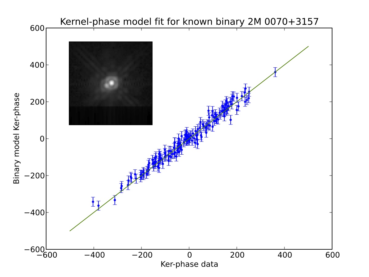
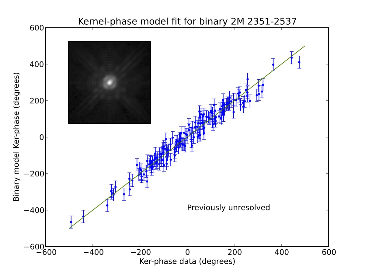
Figure 3: Examples of kernel-phase binary fit results on two ultracool dwarfs observed with HST/NIC1 in the F110W filter. Left: 2M 0070+3157 is a known binary, for which the companion was discovered from visual examination of the image. Right: 2M 2351-2537 is a previously unknown binary, that cannot be resolved in the direct image. The kernel-phase analysis produces a signal of comparable magnitude in either case.

A systematic revisit of a homogeneous sample of $\sim$80 nearby L-dwarfs previously observed with HST/NICMOS was performed by [15] in two filters (F110W and F170M) using the kernel-phase approach outlined in this paper. This study permitted a search for companions down to projected separations of $\sim$1 AU, revealed new binary candidates and provided improved relative astrometry for all known binaries.

After extraction, the kernel-phases are used as constraints in a 3-parameter binary model (separation, position angle and contrast). Conventional likelihood analysis and/or Monte-Carlo simulations provide a binary solution or contrast detection limits. Figure 3 shows two examples of kernel-phase data sets plotted against their best fit binary model.

4.2 Ground-based AO

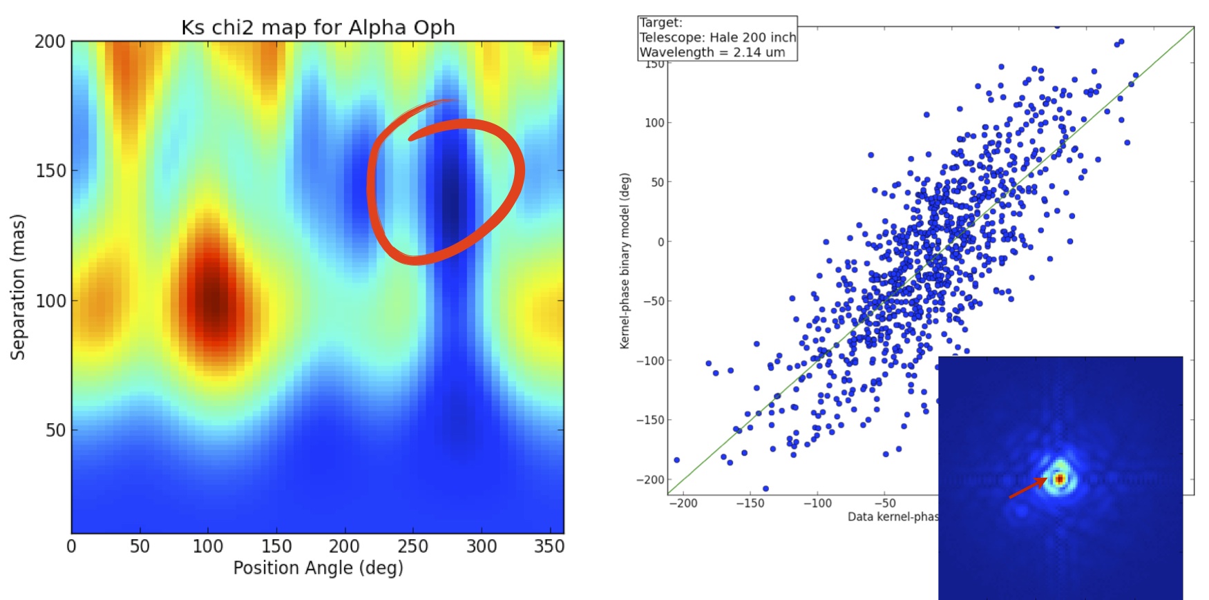
Figure 4: Example of kernel-phase result obtained on ground based AO data. Left: map of the $\chi^{2}$ in the position angle - angular separation space for $\alpha$-Ophiucus, observed with PHARO at the Palomar Hale Telescope, using the model shown in Fig. 2. A red circle highlights the location of the minimum $\chi^{2}$. Right: correlation plot between the kernel-phase data and the binary model for the corresponding location in the $\chi^{2}$ space. The image snippet shows (red arrow) that the 30:1 companion is apparently invisible, hidden under the first diffraction ring.

Application of the method is however not restricted to HST/NICMOS images and can also be applied to ground based AO data, assuming that the on-axis AO correction produces a Strehl better than $\sim$50 %. Fig. 4 showcases one example of result achieved using the model of the Palomar Hale PHARO medium cross pupil introduced in Sec. 3.

The target, $\alpha$-Ophiucus, is a well known binary with a well characterized, eccentric orbit with an 8.6 year period [3]. The kernel-phase analysis of multiple PHARO frames acquired in the K-band revealed the presence of the 30:1 contrast companion at a position angle 274.6^∘, but at an angular separation 136.1 mas ($\sim 1.5\lambda/D$), that is directly underneath the first diffraction ring. The companion, invisible in the direct image, is clearly detected using this approach. The position is in very good accordance with the ephemerides of the orbit.

5 Interferometric imaging with an ELT

The self-calibrating properties of interferometric observables like closure-phase and kernel-phase make it possible to produce images of sources, with resolving power better than what the formal diffraction limit ($\lambda/D$) dictates: a regime called super-resolution. Well known examples include images of complex sources such as pinwheel nebulae [17] obtained by masking the Keck Telescope with a partially redundant annular mask. For an ELT with a 30-meter baseline diameter observing in the near IR ($\lambda=1.6\mu m$), imaging with a resolution of $\sim 5$ mas or less offers fantatic possibilities over a wide range of astrophysical science cases.

For the most part, the design of interferometric masks for imaging has been guided by the widely used designs of Golay [1]. These designs provide a series of compact solutions using three-fold symmetry that maximize the $(u,v)$-coverage while ensuring non-redundancy.

$(u,v)$-coverage is indeed an important factor for successful imaging of complex sources with an interferometer. While it is always possible to increase this coverage with aperture synthesis techniques, the discussion is restricted to the analysis of a single snapshot Fizeau image, such as one acquired with a mask in the pupil of an instrument behind AO. The imaging capability is entirely dictated by the number of independent observables (visibilities and kernel-phases) that can be extracted from the snapshot.

Because it enables extraction of high-quality observables even for redundant apertures, the notion of kernel-phase allows to go beyond the rules of Golay, and has the potential to offer solutions for the imaging of complex sources. A preliminary comparative study of several designs [12] has shown that even when they provide identical $(u,v)$-coverage, some configurations do provide a better phase information recovery rate (the ratio $n_{K}/n_{UV}$).

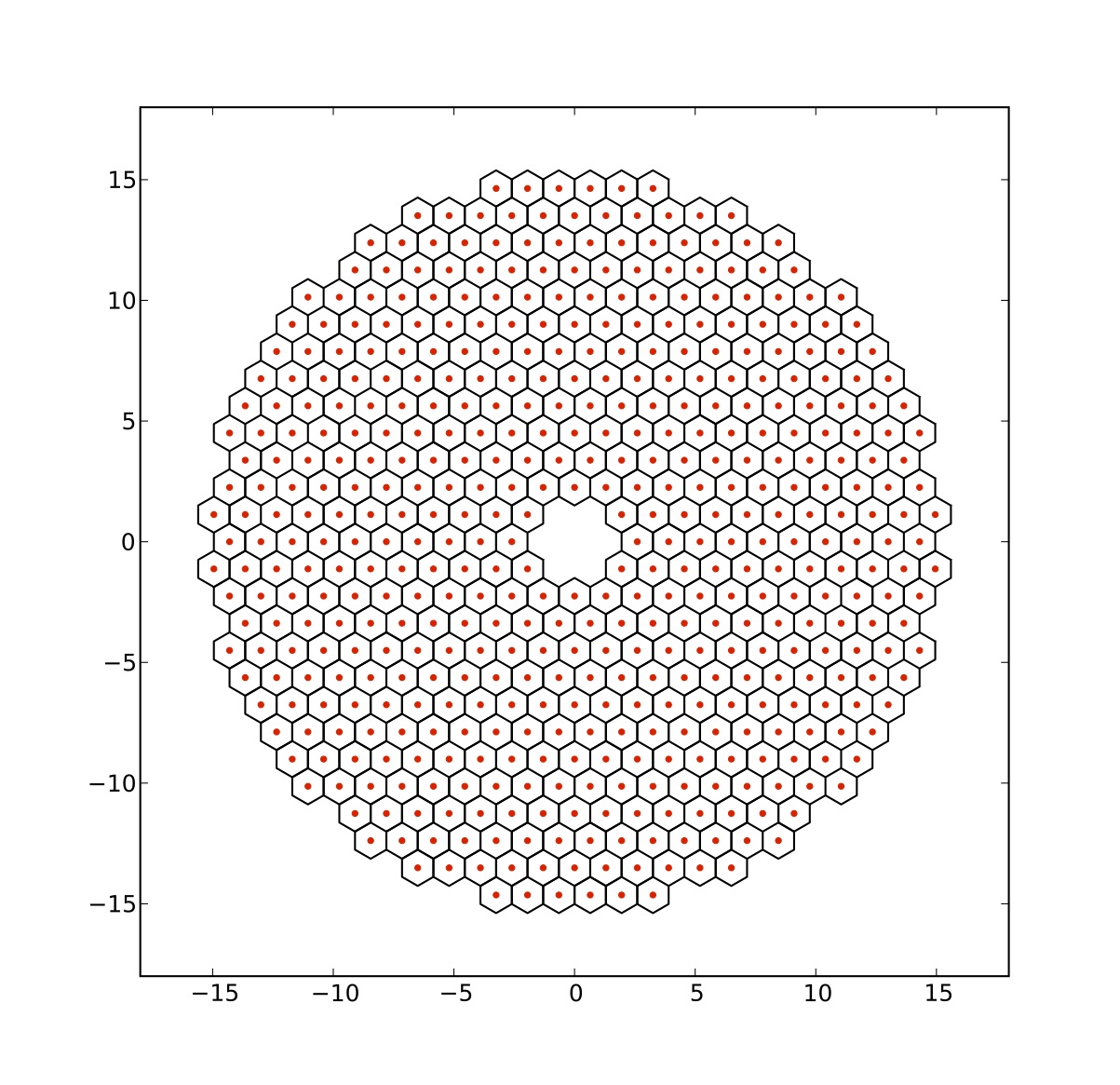
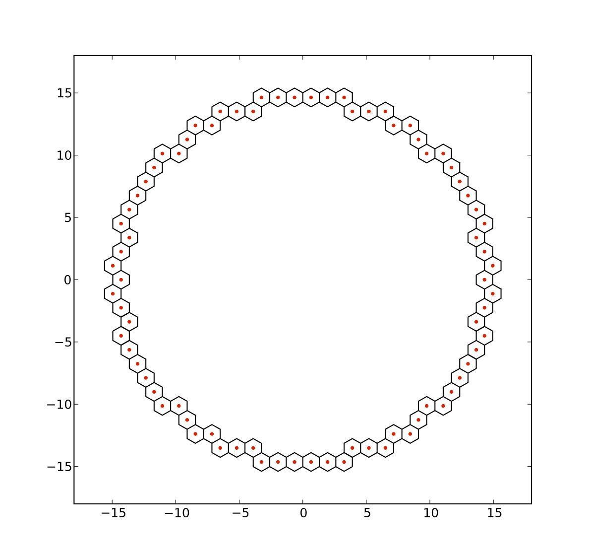
Figure 5: Left: geometry for the 492 segments of the Thirty Meter Telescope (TMT). Right: geometry of the 78 outermost segments that give access to the same $(u,v)$-coverage, but exhibits a better phase information recovery rate.

What comes out of this study is that an annular configuration does seem to provide an optimum, with a $(u,v)$-coverage identical to the full-pupil, but a better yield in terms of phase recovery. The example shown in Fig. 5 compares, for the Thirty Meter Telescope (TMT), the full 492-segment aperture to a subset made of the outermost ring of segments (78). Going through the analysis highlighted in Section 3 for both configurations reveals that both configurations provide access to the same $n_{UV}=972$ distinct sample points in the Fourier plane. Looking for the number of singular values for the phase transfer matrix of these apertures shows that for the full aperture, $n_{K}=726$ kernel-phase relations are available, giving a reasonable phase information recovery rate $\sim 75~{}\%$. The annular configuration exhibits a larger $n_{K}=933$ number of kernel-phase relations, that is a total phase information recovery rate $\sim 96~{}\%$.

Of course, the total throughput of the annular configuration is less favorable ($\sim 16~{}\%$), but remains reasonable in comparison with most non-redundant masks used with great success for imaging purpose today on 8-to-10 meter telescopes. Moreover, because such a mask is used downstream from the AO system, this low throughput does not change the limiting magnitude of the instrument, solely imposed by the upstream AO performance.

Further work is obviously required to verify the benefits of employing one such annular aperture mask on an ELT, and will be the object of publications to come. Nevertheless, this preliminary study means to show that AO-equipped ELTs can be thought of as interferometers with some very interesting imaging capabilities, opening access to a realm of angular separation $\sim 5$ mas in the near IR, that projected on a young association like Taurus (145 pc), allows to probe down to the inner 1 AU region of potential planet host systems.

6 Conclusion

Thinking of the image formation process from an interferometric point of view offers an alternative to the classical object-image convolution problem, with some serious advantages. Using a series of simple examples, the paper shows how the notion of closure-phase can naturally be generalized when one assumes that wavefront errors are small ($\lesssim 1$ radian). The convolution equation can be replaced by a linear model for the phase measured in the Fourier plane. Kernel-phase, a generalization of closure-phase, are associated to singular modes of the phase transfer matrix that propagates pupil phase errors into phase in the Fourier-plane.

Initially envisionned for the processing of narrow-band very high-Strehl data acquired from space, kernel-phase slowly appears to be a quite versatile tool, actually compatible with medium and wide band filters, and quite able to handle reasonably well corrected AO images.

Thinking ahead about the possibilities offered by the large aperture of ELTs, one sees a fair bit of potential for very high angular resolution imaging, using this interferometric framework. Kernel-phase is a powerful tool for high angular resolution imaging that explores a still exclusive region of the parameter space.

References

- [1] Golay, M. 1971, JOSA, 61, 272
- [2] Hayward et al. 2001, PASP, 113, 105
- [3] Hinkley et al. 2011, ApJ, 726, 104
- [4] Kraus et al. 2008, ApJ, 679, 762
- [5] Kraus et al. 2011, ApJ, 731, 8
- [6] Kraus & Ireland 2012, ApJ, 745, 5
- [7] Ireland et al. 2008, ApJ, 678, 463
- [8] Ireland, M. J. 2013, MNRAS, 433, 1718
- [9] Jennison, R. C. 1958, MNRAS, 118, 276
- [10] Marois et al. 2006, ApJ, 641, 556
- [11] Martinache, F. 2010, ApJ, 724, 464
- [12] Martinache, F. 2012, SPIE, 8445, 04
- [13] Martinache et al. 2012, PASP, 124, 1288
- [14] Monnier J. D., 2000, Principles of Long Baseline Stellar Interferometry, 203
- [15] Pope et al. 2013, ApJ, 767, 110
- [16] Tuthill et al. 2006, SPIE, 6272, 103
- [17] Tuthill et al. 2008, ApJ, 675, 698