Periodicity in some light curves of the solar analogue V352 CMa

Abstract

Aims. Our aim was to study the light curve periodicity of the solar analogue V352~CMa and in particular show that the presence or absence of periodicity in low amplitude light curves can be modelled with the Continuous Period Search (CPS) method.

Methods. We applied the CPS method to 14 years of V-band photometry of V352 CMa and obtained estimates for the mean, amplitude, period and minima of the light curves in the selected datasets. We also applied the Power Spectrum Method (PSM) to these datasets and compared the performance of this frequently applied method to that of CPS.

Results. We detected signs of a $11.7\pm 0.5$ year cycle in in the mean brightness. The long–term average photometric rotation period was $7.24\pm 0.22$ days. The lower limit for the differential rotation coefficient would be $|k|>0.12$, if the law of solar surface differential rotation were valid for V352~CMa and the period changes traced this phenomenon. Signs of stable active longitudes rotating with a period of $7.157\pm 0.002$ days were detected from the epochs of the light minima with the Kuiper method. CPS performed better than the traditional PSM, because the latter always used a sinusoidal model for the data even when this was clearly not the correct model.

1 Introduction

V352~CMa (HD~43162) was among the first 384 bright extreme ultraviolet sources detected by the ROSAT satellite (Shara et al., 1993). Metallicity and space motion indicated that it belongs to the young disk population (Eggen, 1995). It was included into the list of 38 nearby young single solar analogs having ages between 0.2 and 0.8 Gyr (Gaidos, 1998). We collected some of its physical parameters into Table 1. Strong Ca H&K emission ($R^{\prime}_{\mathrm{HK}}$), high X-ray luminosity ($R_{\mathrm{X}}$) and rapid rotation ($v\sin{i}$) indicate that it is a young star. The high lithium abundance also supports this (Gaidos, 1998; Santos et al., 2004a). However, the age and metallicity ([Fe/H]) estimates are inconsistent (Table 1). Except for Gaidos et al. (2000) and Gaidos & Gonzalez (2002), the effective surface temperature ($T_{\mathrm{eff}}$) and gravity ($\log{g}$) estimates agree and support the spectral type G6.5 V (Gray et al., 2006).

V352~CMa was classified as a member of a stellar kinematical group (hereafter SKG) of 19 stars by Jeffries & Jewell (1993). Later, it has been identified as a member another group IC 2391. This more recently identified SKG contains 29 stars. The estimated age of IC 2391 is 45 Myr (Nakajima et al., 2010; Maldonado et al., 2010; Nakajima & Morino, 2012). However, only two stars in IC 2391 were among the 19 members of the original SKG defined by Jeffries & Jewell (1993). These two stars are V352~CMa and LQ~Hya. This indicates how difficult it is to confirm the membership in any particular SKG. Christian et al. (2003) observed an extreme ultraviolet flare in a M3.5 V star (EUVE J0613–23.9B) located 2$\aas@@fstack{\prime}$5 away from V352~CMa (EUVE J0613–23.9). We noticed that this M3.5 V star is the same object that was later identified as the binary companion of V352~CMa (Raghavan et al., 2010). About 90% of the ROSAT source positions were within 1′, and 100% were within 2$\aas@@fstack{\prime}$1, of the catalogued positions (Shara et al., 1993). The 2$\aas@@fstack{\prime}$5 distance between V352~CMa and its M3.5 companion is close to the latter 2$\aas@@fstack{\prime}$1 limit. This companion had no influence to our photometry, because the diameter of the focal-plane diaphragm is only 55″.

V352~CMa was in the sample of 11 new stars, where a debris disk was detected using the Spitzer Space Telescope data (Kóspál et al., 2009). However, it was the only star in this sample without a known planet. Cutispoto et al. (1999) determined the photometric rotation period of V352~CMa, $P_{\mathrm{phot}}=7\aas@@fstack{d}2\pm 0\aas@@fstack{d}2$, from a light curve with a low $0.03$ peak to peak amplitude. Gaidos et al. (2000) detected no periodicity in their photometry, which were the same data as our first season of photometry. Hipparcos photometry revealed no periodicity (Koen & Eyer, 2002, n=228 observations). Wright et al. (2004) derived $P_{\mathrm{phot}}\approx 8^{\mathrm{d}}$ from the observed $B-V$ and $R^{\prime}_{HK}$ values.

In this research note, we analyse long-term photometry of V352~CMa with CPS (Lehtinen et al., 2011). The previous studies have indicated that periodicity may be present or absent in any part of this photometry. We will show that CPS is an ideal method for analysing this type of challenging data. We also compare CPS to PSM formulated by Horne & Baliunas (1986).

Table 1: Physical parameters of V352~CMa

$T_{\mathrm{eff}}$		$\log{g}$		$v_{\mathrm{rad}}$		$v\sin{i}$		[Fe/H]		Age		$R^{\prime}_{\mathrm{HK}}$		$R_{\mathrm{X}}$
${\mathrm{[K]}}$	Ref	${\mathrm{[cm\leavevmode\nobreak\ s^{-2}]}}$	Ref	${\mathrm{[km\leavevmode\nobreak\ s^{-1}]}}$	Ref	${\mathrm{[km\leavevmode\nobreak\ s^{-1}]}}$	Ref		Ref	[Myr]	Ref		Ref		Ref
$5480$	7	$4.57$	10	$22.7\pm 0.7$	1	$6\pm 2$	6	$-0.15$	4	$200-800$	5	$-4.40$	7	$-4.26$	5
$5593$	8	$4.10$	11	$21.69\pm 0.16$	2	$5.7$	7	$-0.16$	9	$70-800$	7	$-4.40$	12	$-4.31$	7
$5630$	10	$4.48$	13	$22.6\pm 0.6$	3	$5.49$	13	$-0.02$	10	$575$	12	$-4.48$	18	$-4.29$	21
$5473$	11	$4.49$	18	$21.3-21.8$	6	$9.63$	22	$-0.11$	11	$<1000$	14	$-4.39$	21	$-4.39$	22
$5633$	13	$4.52$	23	$21.7$	7			$-0.01$	13	$<6500$	19
$5585$	15			$21.9\pm 0.2$	16			$-0.10$	15	$33-35,280$	21
$5571$	18			$21.91\pm 0.09$	17			$-0.10$	19	$5286$	24
$5584$	19			$22.23\pm 0.09$	21			$-0.04$	20	$<45$	25
$5590$	23							$0.02$	23
								$0.02$	24

(1) Beavers & Eitter (1981); (2) Andersen et al. (1985); (3) Beavers & Eitter (1986); (4) Eggen (1995); (5) Gaidos (1998); (6) Cutispoto et al. (1999); (7) Gaidos et al. (2000); (8) Decin et al. (2000); (9) Haywood (2001); (10) Santos et al. (2001); (11) Gaidos & Gonzalez (2002); (12) Wright et al. (2004); (13) Santos et al. (2004a); (14) Santos et al. (2004b); (15) Nordström et al. (2004); (16) Gontcharov (2006); (17) Abt & Willmarth (2006); (18) Gray et al. (2006); (19) Holmberg et al. (2009); (20) Árnadóttir et al. (2010); (21) Maldonado et al. (2010); (22) Martínez-Arnáiz et al. (2010); (23) Brugamyer et al. (2011); (24) Fernandes et al. (2011); (25) Nakajima & Morino (2012)

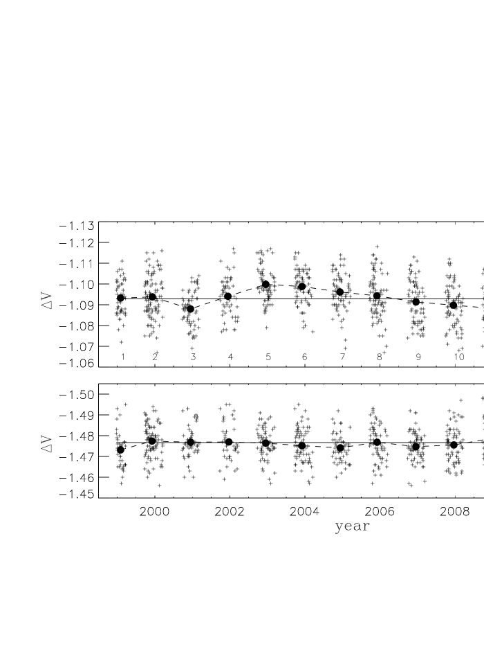
Figure 1: Differential photometry. (a) All $\Delta V_{\mathrm{S-C}}$ data (crosses), their mean level (continuous line) and the seasonal $\Delta V_{\mathrm{S-C}}$ means (filled circles) connected with dashed lines. (b) All $\Delta V_{\mathrm{K-C}}$ data. The magnitude scale and the notations are as in (a)

2 Observations

The photometry of our target star S=V352~CMa was obtained with the automated T3 0.4 m photoelectric telescope (APT) at Fairborn Observatory in Arizona. The observations were made between December 23rd, 1998 (HJD=2451170.8) and March 17th, 2012 (HJD=2456003.6) during 14 observing seasons. The comparison star was C=HD~43879 (F5V, $V=7.26$), which is a visual double with $V=7.3$ and $11.2$ components. Both components are included in the 55″focal-plane diaphragm of the photometer, because their angular separation is only 6.7″. The check star was K=HD~43429 (K1 III, $V=5.99$). The standard Johnson differential magnitudes, $\Delta V_{\mathrm{S-C}}$, are shown in Fig. 1a. The mean ($m$) and the standard deviation ($s$) of these $n=1257$ observations were $m=-1.0929$ and $s=0.0096$. The lower panel displays the $\Delta V_{\mathrm{K-C}}$ differential magnitudes. The standard deviation of these $\Delta V_{\mathrm{K-C}}$ observations ($n=1027$) gave an internal accuracy estimate of $0.0079$. We used this accuracy estimate to test the constant brightness hypothesis for $\Delta V_{\mathrm{S-C}}$. The result, $\chi^{2}=1854$, for these $\Delta V_{\mathrm{S-C}}$ observations ($n=1257$) indicated that the brightness changes of V352~CMa were real. There were also clear trends in the $n=14$ seasonal $\Delta V_{\mathrm{S-C}}$ means having $s=0.0036$ (Fig. 1a: filled circles). The respective seasonal $\Delta V_{\mathrm{K-C}}$ means were more stable with $s=0.0016$ (Fig. 1b: filled circles). More detailed information of the operation of the T3 0.4 m APT and the data reduction procedures can be found, e.g. in Henry (1999) and Fekel & Henry (2005).

Figure 2: The data and light curves of all independent datasets ($IND(\tau)=1$). All notations are explained in the 5th paragraph of Sect. 3

3 CPS results

CPS divided the data into segments (SEG) and datasets (SET). There were 14 segments (i.e. seasons). The maximum length of a dataset was $\Delta T_{\rm max}=30^{\mathrm{d}}$. Each dataset had to contain at least $n\geq n_{\rm min}=12$ observations $y_{i}=\Delta V_{\mathrm{S-C}}(t_{i})$. The CPS results correlate for temporally overlapping datasets, because they contain common data. To eliminate such correlation, we selected the sequence of independent datasets with no common data. The notations ${\rm IND}(\tau)=1$ and 0 are used for independent and not independent (i.e. overlapping) datasets, respectively. Our notation for the mean of the $n$ observing times $t_{i}$ of a dataset is $\tau$.

The CPS model is a $K$:th order Fourier series

$$\hat{y}(t_{i})=\hat{y}(t_{i},\bar{\beta})=M+\sum_{k=1}^{K}{[B_{k}\cos{(k2\pi ft_{i})}+C_{k}\sin{(k2\pi ft_{i})}]}.$$

Of the free parameters $\bar{\beta}=[M,B_{1},..,B_{K},C_{1},...,C_{K},f]$, the physically meaningful ones are the mean, $M(\tau)$ and the period, $P(\tau)=f^{-1}(\tau)$. The other free parameters $B_{1},...,B_{\rm K},C_{1},...,C_{K}$ give the total amplitude of the model, $A(\tau)$, as well as the epochs of the primary and secondary minima in time, $t_{\rm min,1}(\tau)$ and $t_{\rm min,2}(\tau)$. CPS uses the Bayesian information criterion to choose the best modelling order $K$ for each dataset. We tested orders $0\leq K\leq 2$. The total number of modelled datasets was 485. Of these, no periodicity was detected in 178 datasets ($K=0$), where the best model was constant brightness $\hat{y}(t_{i})=M(\tau)$. Periodicity was detected in 307 datasets. The best orders were $K=1$ in 170 datasets and $K=2$ in 137 datasets.

The error estimates for $M(\tau)$, $A(\tau)$, $P(\tau)$, $t_{\rm min,1}(\tau)$ and $t_{\rm min,2}(\tau)$ were determined with the bootstrap method. Bootstrap was also used to identify the reliable or unreliable light curve parameter estimates. Our notations are $R(\tau)=0=$ reliable estimate and $R(\tau)=1=$ unreliable estimate. The CPS results are published only electronically. We use the format specified in Lehtinen et al. (2011), where a detailed description of CPS can be found. The CPS results for different parameters are summarised below.

	${\rm IND}(\tau)=1$	${\rm IND}(\tau)=1$	${\rm IND}(\tau)=0$	${\rm IND}(\tau)=0$
	${\rm R}(\tau)=0$	${\rm R}(\tau)=1$	${\rm R}(\tau)=0$	${\rm R}(\tau)=1$
$M(\tau)$	$n=39$ $[\blacksquare]$	$n=14$ $[\Box]$	$n=331$ $[\times]$	$n=101$ $[\times]$
$A(\tau)$	$n=20$ $[\blacksquare]$	$n=14$ $[\Box]$	$n=172$ $[\times]$	$n=101$ $[\times]$
$P(\tau)$	$n=20$ $[\blacksquare]$	$n=14$ $[\Box]$	$n=172$ $[\times]$	$n=101$ $[\times]$
$t_{\mathrm{min,1}}(\tau)$	$n=20$ $[\blacksquare]$	$n=14$ $[\Box]$	$n=172$ $[\times]$	$n=101$ $[\times]$
$t_{\mathrm{min,2}}(\tau)$	$n=5$ $[\blacktriangle]$	$n=8$ $[\triangle]$	$n=65$ $[\times]$	$n=47$ $[\times]$

The symbols in brackets are used in Fig. 3, where error bars are displayed only for ${\rm IND}(\tau)=1$ datasets.

CPS also gave the time scale of change of the light curve, $T_{\mathrm{C}}(\tau)$, for all 370 reliable models. The light curve of V352~CMa changed before the end of the segment only in 37 datasets, where the $T_{\mathrm{C}}$ mean was 51 days. This mean exceeded 65 days in the other 333 datasets, where the light curve did not change before the segment end. Both values indicated that the applied dataset length, $\Delta T_{\mathrm{max}}=30^{\mathrm{d}}$, gave reliable CPS results.

The light curves of independent datasets are shown in Fig. 2. The continuous lines display the periodic curves ($K\geq 1$). The phases were first computed from $\phi_{1}=\mathrm{FRAC}[(t-t_{\mathrm{min,1}}(\tau))/P(\tau)]$, where $\mathrm{FRAC}[x]$ removes the integer part of its argument $x$. Then the phases $\phi_{\mathrm{al,1}}$ of the $t_{\mathrm{min,1}}(\tau)$ epochs were computed from the constant period ephemeris HJD $2451178.1245+7\aas@@fstack{d}158$E. Finally, the data and the light curves were plotted as a function of $\phi=\phi_{1}+\phi_{\mathrm{al,1}}$. The dashed lines display the aperiodic curves ($K=0$), where the “phases” are $\phi_{i}=(t_{i}-t_{1})/(t_{n}-t_{1})$. The SEG, SET, $\tau$ and $R(\tau)$ values are also given.

Figure 3: (a) mean $M(\tau)$, (b) amplitude $A(\tau)$, (c) period $P(\tau)$ and (d) phases of the primary $t_{\mathrm{min,1}}(\tau)$ and secondary $t_{\mathrm{min,2}}(\tau)$ minima. The symbols are explained in the 3rd paragraph of Sect. 3. The horizontal lines in (c) denote the $P_{\mathrm{w}}\pm 3\Delta P_{\mathrm{w}}$ level. The phases in (d) were calculated from HJD $2451178.1245+7\aas@@fstack{d}158$E.

The long-term $M(\tau)$ and $A(\tau)$ changes of V352~CMa are shown in Fig. 3, panels a) and b). PSM has been applied to search for activity cycles in chromospheric Ca II H&K emission line data (e.g. Baliunas et al., 1995). Rodonò et al. (2000) applied this method to the following light curve parameters: $M(\tau)$ (axisymmetric part of spot distribution), $A(\tau)$ (non-axisymmetric part of spot distribution), $M(\tau)-A(\tau)/2$ (minimum spotted area) or $M(\tau)+A(\tau)/2$ (maximum spotted area). We applied PSM to the same independent and reliable estimates of V352~CMa. The false alarm probability of the best cycle, $P_{\mathrm{C}}=11\overset{\text{y}}{.}7\pm 0\overset{\text{y}}{.}5$ for the $n=39$ values of $M(\tau)$, was $F=0.01$. The cycles for the $n=20$ values of $A(\tau)$, $M(\tau)-A(\tau)/2$ and $M(\tau)+A(\tau)/2$ reached only $F\geq 0.26$.

The weighted mean of the independent and reliable $P(\tau)$ $(n=20)$ estimates was $P_{\mathrm{w}}\pm\Delta P_{\mathrm{w}}=7\aas@@fstack{d}24\pm 0\aas@@fstack{d}22$. This range of period changes, $P_{\mathrm{w}}\pm 3\Delta P_{\mathrm{w}}$, (Fig. 3c: dotted lines) gave $Z=6\Delta P_{\mathrm{w}}/P_{\mathrm{w}}=0.19\equiv 19$ % (Lehtinen et al., 2011, Eq. 14). The average of the light curve half amplitude $A(\tau)/2$ in these datasets was only $0.011$. The accuracy of the photometry, $\sigma_{\mathrm{N}}=0.007$, gave an amplitude to noise ratio of $A/N\la 2$. Even if the spurious period changes were $Z_{\mathrm{spu}}\geq 0.15$, the estimated real physical changes could be $Z_{\mathrm{phys}}=(Z^{2}-Z_{\mathrm{spu}}^{2})^{-1/2}\approx 0.12$ (Lehtinen et al., 2011, Table 3 and Eq. 15). We assumed that the solar law of surface differential rotation could be applied to V352~CMa and that the period $P(\tau)$ changes could be used to trace surface differential rotation. We used $k\approx Z_{\mathrm{phys}}/h$, where the minimum and maximum latitudes of spot activity were $b_{\mathrm{min}}$ and $b_{\mathrm{max}}$, and $h=\sin^{2}{b_{\mathrm{max}}}-\sin^{2}{b_{\mathrm{min}}}$ (Jetsu et al., 2000). The maximum value, $h=1$, would be reached, if spots were formed at all latitudes between the equator and pole of V352~CMa. All other alternatives give $h<1\Rightarrow|k|>Z_{\mathrm{phys}}\approx 0.12$. This result was comparable to the solar value $k=0.20$, because sunspots form at latitudes $\pm 30^{\mathrm{o}}$ (i.e. $h=0.25$).

We applied the non-weighted Kuiper test (Jetsu & Pelt, 1996) to the reliable primary minima $t_{\mathrm{min,1}}(\tau)\leavevmode\nobreak\ (n=20)$ of independent datasets. The test range was between $0.85P_{\mathrm{w}}=6\aas@@fstack{d}0$ and $1.15P_{\mathrm{w}}=8\aas@@fstack{d}1$. The critical level of the best period $P_{\mathrm{al,1}}=7\aas@@fstack{d}158\pm 0\aas@@fstack{d}002$ was $Q=0.004$. The test for the reliable $t_{\mathrm{min,1}}(\tau)$ and $t_{\mathrm{min,2}}(\tau)$ $(n=25)$ of all independent datasets gave the same result, $P_{\mathrm{al,1,2}}=7\aas@@fstack{d}158\pm 0\aas@@fstack{d}002$, but the critical level of this periodicity was lower, $Q=0.056$. The phases of all primary and secondary minima are shown in Fig. 3d using the ephemeris HJD $2451178\aas@@fstack{d}1245+7\aas@@fstack{d}158$E. The phases of $t_{\mathrm{min,1}}$ estimates were very stable between 1998 and 2009 (Fig. 3d: Filled squares). However, this long–lived structure vanished after 2009 when the light curve amplitudes $A(\tau)$ decreased.

We then applied PSM to all datasets analysed with CPS. The abbreviation “C₀” was used for the cases: $P_{\mathrm{CPS}}-\sigma_{P_{\mathrm{CPS}}}\leq P_{\mathrm{PSM}}\leq P_{\mathrm{CPS}}+\sigma_{P_{\mathrm{CPS}}}$. Our results were

Criterion	$K=1$ or 2 $\leavevmode\nobreak\ [\mathrm{\%}]$	$K=1\leavevmode\nobreak\ [\mathrm{\%}]$	$K=2\leavevmode\nobreak\ [\mathrm{\%}]$
$A(\tau)>0$	$173/307\equiv 56$	$141/170\equiv 83$	$32/137\equiv 23$
$A(\tau)>0.015$	$129/240\equiv 54$	$97/112\equiv 87$	$32/128\equiv 25$
$A(\tau)>0.030$	$15/40\equiv 38$	$3/3\equiv 100$	$12/37\equiv 32$
$F<0.5$	$152/258\equiv 59$	$126/149\equiv 85$	$26/109\equiv 24$
$F<0.1$	$52/86\equiv 60$	$41/42\equiv 98$	$11/44\equiv 25$
$F<0.05$	$25/36\equiv 69$	$18/18\equiv 100$	$7/18\equiv 39$

Case $C_{0}$ was true only in 56% cases for all periodicity detections ($n=307:K=1$ or 2, $A(\tau)>0.00$). This occurred more often for $K=1$ (83%) than for $K=2$ (23%) models. These fractions increased for higher amplitude, $A(\tau)>0.015$, light curves. For the highest amplitudes, $A(\tau)>0.030$, case $C_{0}$ was true for all $K=1$ models (100%), but not for all $K=2$ models (32%). As expected, the probability for case $C_{0}$ being true also increased when the false alarm probability $F$ decreased. For $F<0.05$, case $C_{0}$ was true for all $K=1$ models (100%), but again not for all $K=2$ models (39%). In conclusion, PSM did not always detect the correct period for the $K=2$ light curves. This occurred also for high amplitudes $A(\tau)$ or for small false alarm probabilities $F$.

4 Conclusions

We wanted to test the performance of CPS and applied it to the low amplitude light curves of V352~CMa. These data were challenging, because the dispersions of the $\Delta V_{\mathrm{V-C}}$ and $\Delta V_{\mathrm{K-C}}$ magnitudes were comparable (Figs. 1ab). In a total of 485 datasets, CPS detected no periodicity in 178 $\equiv$ 37% datasets. Comparison of CPS and PSM revealed that both methods gave the same best periods for high amplitude to noise ratio light curves, but only if the correct model for the data was a sinusoid $(K=1)$. The best periods were mostly not the same for the $K=2$ models – not even for the higher $A/N$ light curves. We conclude that if the period $P(\tau)$ or the model order $K$ are not correct, then the $M(\tau)$, $A(\tau)$, $t_{\mathrm{min,1}}$ and $t_{\mathrm{min,2}}$ estimates are in many cases also not correct.

We detected signs of an activity cycle, $P_{\mathrm{C}}=11\overset{\text{y}}{.}7\pm 0\overset{\text{y}}{.}5\leavevmode\nobreak\ (F=0.010)$, in the mean $M(\tau)\leavevmode\nobreak\ (n=39)$. However, it was only $1^{\mathrm{y}}$ shorter than the time span of the data, $\Delta T=13\overset{\text{y}}{.}0$. The $P(\tau)$ period changes could be mostly spurious $(Z_{\mathrm{spu}}>0.15)$ due to low $A/N$ ratio (Lehtinen et al., 2011, Table 3). If the law of solar differential rotation were valid in V352~CMa, and these $P(\tau)$ changes traced this phenomenon, the surface differential rotation coefficient would be $|k|>Z_{\mathrm{phys}}\approx 0.12$. The Kuiper method detected an active longitude rotating with a period of $P_{\mathrm{al,1}}=7\aas@@fstack{d}158\pm 0\aas@@fstack{d}002\leavevmode\nobreak\ (Q=0.004)$. This long–lived structure was present between 1998 and 2009, but vanished when the amplitudes of the light curves fell close to zero in 2010.