Horizon Run 3: Topology as a Standard Ruler

Abstract

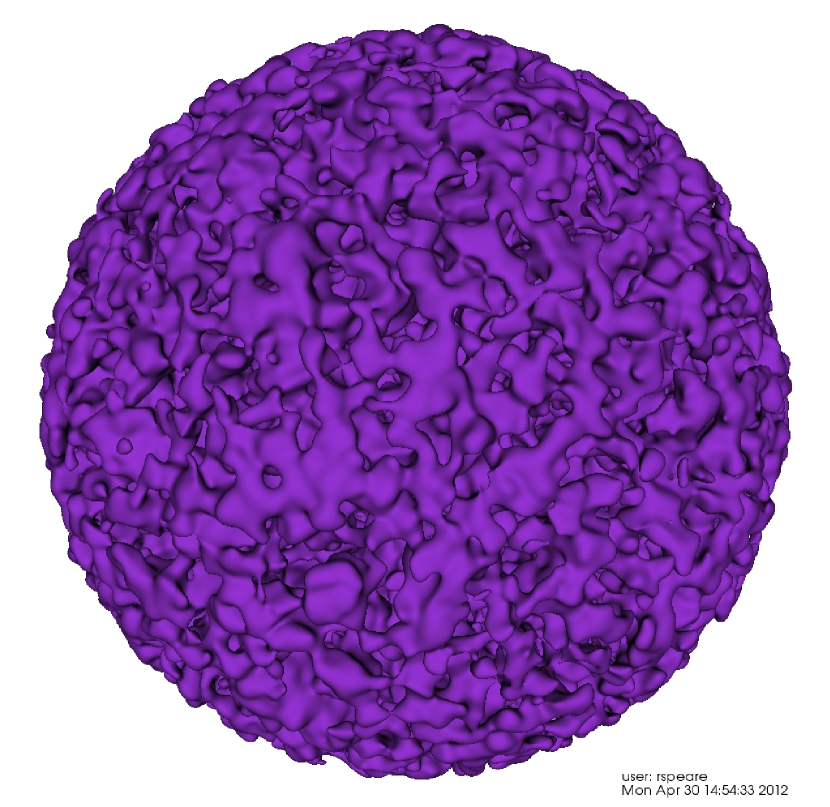
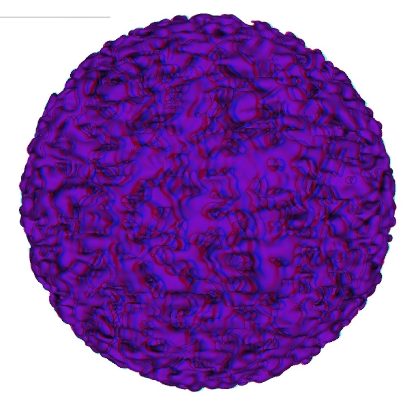
We study the Physically Self Bound Cold Dark Matter Halo distribution which we associate with the massive galaxies within the Horizon Run 3 to estimate the accuracy in determination of the cosmological distance scale measured by the topology analysis. We apply the routine “Contour 3D” to 108 Mock Survey of $\pi$ steradians out to redshift z = 0.6, which effectively correspond to the SDSS-III BOSS survey, and compare the topology with that of a Gaussian Random Phase Field. We find that given three separate smoothing lengths $\lambda=$ 15, 21, and 34 $h^{-1}{\rm Mpc}$, the least $\chi^{2}$ fit genus per unit volume g yields a 1.7 % fractional uncertainty in smoothing length and angular diameter distance to $z=0.6$. This is an improvement upon former calibrations of and presents a competitive error estimate with next BAO scale techniques. We also present three dimensional graphics of the Horizon Run 3 spherical mock survey to show a wealth of large-scale structures of the universe that are predicted in surveys like BOSS.

1. Introduction

The most popular model for the generation of primordial density fluctuations is the inflationary scenarios (Guth, 1981; Linde, 1982; Albrecht & Steinhardt, 1982; Linde, 1983). This model assumes primordial density perturbations of Gaussian random phase and it has been shown that such initial conditions produce a sponge-like topology on large scales (Gott, Melott, & Dickinson, 1986, 1987). At such scales, where the power spectrum has not been transformed by nonlinear growth, the topology of structure in the early universe is well preserved, and small deviations from random phase predictions give important information about primordial non-gaussianity, biased galaxy formation, and non-linear clustering (Matsubara, 1994; Park, et al., 2005a; Park et al., 2012; Park & Gott, 1991; Park et al., 1998).

The genus statistic is central to these studies, and is now a well-tested quantitative measure (Gott, Melott, & Dickinson, 1986; Gott, Weinberg, & Melott, 1987; Hamilton, Gott, and Weinberg, 1986; Gott et al., 1989; Vogeley et al., 1994; Hikage et al., 2002, 2003; Choi et al., 2010; Park, et al., 2005a; Park et al., 2005b), having been applied to both the SDSS LRG sample (Gott et al., 2009; Strauss et al., 2002; Eisenstein et al., 2011), and the CMB (Park et al., 1998). It’s utility lies in the existence of the “genus curve”, an analytical expression for genus as a function of density, which allows comparison of observed topology with that expected from a standard big bang inflationary model (Hamilton, Gott, and Weinberg, 1986).

So far, fitting the Gaussian random phase (hereafter, GRP) genus curve to mock surveys in a $\Lambda$CDM cosmology has been remarkably successful. The genus has now been suggested as a cosmic standard ruler (Park & Kim, 2010) and a means for probing dark energy (Park & Kim, 2010; Zunckel, Gott, & Lunnan, 2011; Slepian, Gott, & Zinn, 2013). The Baryon Acoustic Oscillation (BAO) feature, detectable in the power spectrum and galaxy two point correlation function, is the established “standard ruler” (Anderson et al., 2012), with a reported fractional uncertainty in angular diameter distance to $z=0.6$ of 1.1 % expected for the SLOAN survey when completed. Now, with the introduction of ever larger galaxy samples, such as the CMASS Data Release 10 sample of the SDSS-III Baryon Oscillation Spectroscopic Survey (BOSS), topology is becoming another attractive technique for probing the expansion of the universe and constraining the equation of state of Dark Energy. We apply the genus to 108 LRG mock surveys, derived from the Horizon Run 3 $N$-body Simulations (Kim et al., 2011), in order to ascertain the statistical accuracy of said “topological distance measure”.

2. The Genus Statistic

Gott, Melott, & Dickinson (1986) presented the genus as a reliable description of topology. Traditionally, the genus comes from the Gauss-Bonnet theorem, which states that the integral of gaussian curvature $K=1/({r_{1}r_{2}})$ (where $r_{1}$ and $r_{2}$ are the principle radii) over a compact two-dimensional surface is given by

$$\int KdA=4\pi(1-G_{b}).$$ (1)

We use a slightly altered form of the Gauss-Bonnet genus, $G=G_{b}-1$, so that it has a more intuitive meaning for Cosmology

$$G=(\rm{\#of\ doughnut\ holes})-(\rm{\#of\ isolated\ regions}).$$ (2)

See Park et al. (2013) for relation to the Euler characteristic and the Betti numbers. With this definition, the genus of a sphere is $G=-1$; a toroid, $G=0$; three isolated spheres, $G=-3$; a figure 8 pretzel, $G=1$ (two holes, one isolated body). Essentially, the genus is a measure of connectivity. A highly connected structure – such as a sponge – will have many holes, a single body, and therefore a large, positive genus. A sparse array of objects – a meatball topology (Soneira & Peebles, 1978; Press & Schechter, 1974) – will have many isolated regions, relatively few holes, and therefore a negative genus. An array of isolated voids will also produce a negative genus.

To calculate the genus we smooth the Horizon Run 3 Physically Self Bound Subhalo distribution Kim et al. (2011) with a Gaussian smoothing ball of radius $\lambda$ (Eq. 8).

We picked the most massive physically bound subhalos to match the number density of LRG galaxies projected for the SLOAN III survey when completed. The Horizon Run 3 is a Cold Dark Matter simulation. We make the simple assumption that the most luminous red galaxies will from in the centers of the most massive cold dark matter halos. In the simulation, the most massive subhalos ($>$ 30 CDM particles) are identified that physically bond and not tidally disruptable by larger structures – these we associate with LRG galaxies.

We then create iso-density contour surfaces of the smoothed density distribution, labeling them by $\nu$, which is related to the volume fraction $f$ on the high density side of the contour by

$$f=\frac{1}{\sqrt{2\pi}}\int_{\nu}^{\infty}e^{-x^{2}/2}dx,$$ (3)

Where $x$ is the density parameter. The value $f=50\%$ corresponds to the median volume fraction contour ($\nu=0$). For GRP initial conditions the genus curve is

$$g_{rf}(\nu)=A(1-\nu^{2})e^{-x^{2}/2}.$$ (4)

Where the amplitude $A=(1/2\pi^{2})(\left<k^{2}\right>/3)^{3/2}$, and $\left<k^{2}\right>$ is the average value of the squared wave vector, $k^{2}$ in the smoothed power spectrum (Gott, Melott, & Dickinson, 1986); or, the slope of the two-point correlation function.

The shape of a genus curve, and its deviation from the random phase prediction, can be parametrized by several variables. First, there is the $\chi^{2}$ best fit amplitude, which is measured by fitting the GRP curve ( Eq. 4) to the observed curve. This gives information about the power spectrum and phase correlation of the density fluctuation. Secondly, there are three variables which characterize deviations from a GRF (Park, Gott, & da Costa, 1992):

$$\Delta\nu = \frac{\int_{-1}^{1}g(\nu)\nu d\nu}{\int_{-1}^{1}g_{\rm{rf}}(\nu)\nu d\nu},$$ (5)

$$A_{V} = \frac{\int_{-2.2}^{-1.2}g(\nu)d\nu}{\int_{-2.2}^{-1.2}g_{\rm{rf}}(\nu)\nu d\nu},$$ (6)

$$A_{C} = \frac{\int_{1.2}^{2.2}g(\nu)d\nu}{\int_{1.2}^{2.2}g_{\rm{rf}}(\nu)\nu d\nu},$$ (7)

where $g_{\rm{rf}}$ is the best-fit random phase curve (Eq. 4). $\Delta\nu$ measures any shift in the central part of the genus curve. The GRP curve has $\Delta\nu=0$. A negative value of $\Delta\nu$ is called a meatball shift, caused by a greater prominence of isolated high-density structures, pushing the genus curve to the left. $A_{V}$ and $A_{C}$ measure the relative number of voids and clusters with respect to GRP expectations.

3. The $N$-body Simulations

The Horizon Runs, provided by the Korean Institute of Advanced Study (KIAS), provide some of the best raw material for calibrating topological study of LRG surveys (Park, et al., 2005a; Kim et al., 2011). These $N$-body simulations replicate the topology of the SDSS LRG’s exquisitely (Gott et al., 2009; Eisenstein, et al., 2001). We use the Horizon Run 3 (HR3) dataset exclusively, which adopts a pressureless cold dark matter cosmology with a pure cosmological constant $w_{\Lambda}=-1$. The basic HR3 cosmological parameters were fixed by the WMAP5 data (Spergel et al., 2003; Komatsu et al., 2011; Hinshaw et al., 2013) and the initial linear power spectrum was calculated with the CAMB source code (Lewis & Bridle, 2002). The entire simulation is a cube of 374 billion particles, spanning a volume of $(10.815{~{}h^{-1}}{\rm{Gpc}})^{3}$. Initial redshift was $z=27$ and $N_{\rm step}=600$ discrete timesteps were taken.

3.1. Mock LRG Survey Construction

The selection of cold dark matter halos uses the Friend of Friend algorithm, where separation cut off distance is 20 % of the mean separation distance. To improve cluster identification, HR3 searches for Physically Self Bound (PSB) subhalos that are gravitationally self-bound and not tidally disruptable (Kim & Park, 2006). This provides a substantial increase in the similiarity between simulation and observational data, as these dark matter subhalos are sites for LRG formation.

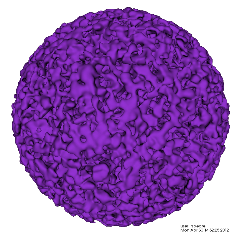
To simulate the SDSS survey dimensions, HR3 places 27 observers evenly within its cubical volume and allows each observer to see out to a redshift of $z<0.7$. This crates 27 independent, non-overlapping spherical regions. The co-moving positions and velocities of all CDM particles are saved as they cross their past light cone and PSB subhalos are identified from this data. In preparation for the SDSS-III LRG catalogue, it was assumed that a volume-limited sample would yield a constant number density of $3\times 10^{-4}(h^{-1}{\rm Mpc})^{3}$. In order to match this prediction, the minimum mass limit of the PSB subhalos was varied with redshift and the absolute minimums were set to $9.75\times 10^{12}~{}{h^{-1}}{\rm M_{\odot}}$. Given these parameters, the physical properties of the HR3 mock surveys match very well with the most recent LRG surveys (Choi et al., 2010; Gott et al., 2009, 2008).

Figure 1.— A spherical Horizon Run 3 Mock survey out to redshift $z=0.7$. The PSB subhalo counts have been smoothed with a Gaussian smoothing ball of $\lambda=34~{}h^{-1}\rm{Mpc}$. See A for 3D plots of the Horizon 3 data.

4. Methods

4.1. Smoothing and Discretization

We smooth the 27 past lightcone PSB subhalo distributions with a gaussian smoothing ball

$$W(\vec{r})=\frac{1}{(2\pi)^{3/2}}e^{-\frac{r^{2}}{2\lambda^{2}}},$$ (8)

smearing structure on scales smaller than $\lambda$. The Mock survey data is placed into a three-dimensional pixel grid of density values, and we choose $\lambda$ to always be greater than $2.5$ pixel sidelengths $s$. For cold dark matter models, smoothing with a Gaussian recovers the topology of the initial density field, provided that the smoothing length $\lambda$ is sufficiently greater than the correlation length $R_{0}$ and non-linear effects are avoided.

4.2. Conversion and Trimming

With this smoothed Mock Survey in hand, we convert from co-moving spherical coordinates to redshift coordinates, using a comoving line of sight distance formula (Hogg, 1999). PSB subhalo peculiar velocities are converted into redshift distortions by

$$\Delta z=\frac{\vec{v_{\rm{r}}}}{c}=\frac{\hat{r}\cdot\vec{v}_{\rm{pec}}}{c},\\$$ (9)

where $\vec{v}_{r}$ is the radial velocity, $\hat{r}$ is the unit radial vector, and $\vec{v}_{\rm pec}$ is the cartesian peculiar velocity of the subhalo. After redshift converting and correcting, we save PSB subhalo counts within a grid of dimensions $650^{3}$, with cubical pixel volume of $s^{3}=(6{~{}h^{-1}}{\rm{Mpc}})^{3}$. The entire grid spans a volume of $(1950{~{}h^{-1}}{\rm{Mpc}})^{3}$.

We then apply an angular mask, splitting the 27 perfectly spherical mock surveys into four quadrants each of $\pi$ steradians and radius $z=0.6$, to approximate the area of sky coverage and depth in the SLOAN III survey. With these $4\times 27=108$ smoothed mock surveys in hand, we calculate the genus using a polygonal approximation scheme developed by Weinberg (1988); Hamilton, Gott, and Weinberg (1986) called “Contour 3D”, which adds up angle deficits at pixel vertices.

5. Using Topology as a Standard Ruler

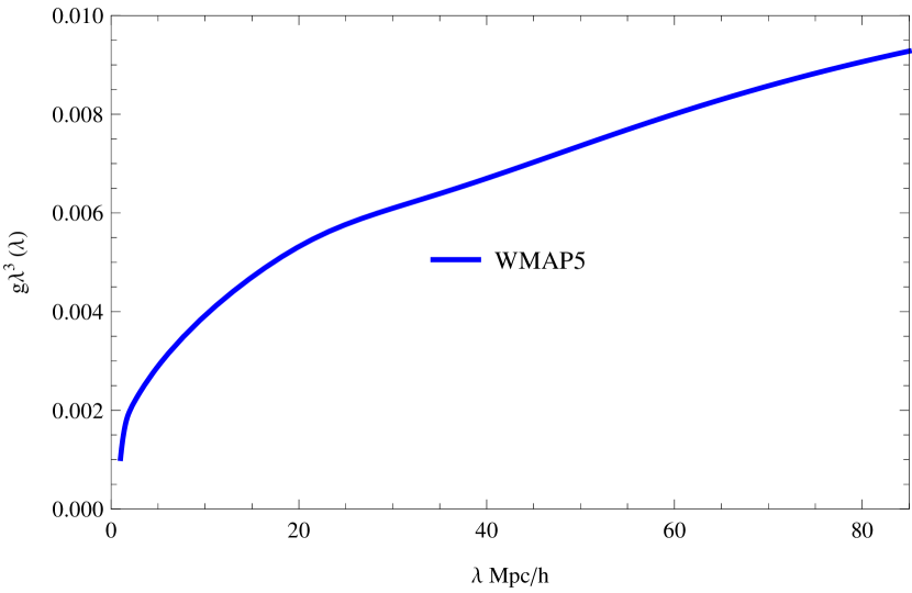
An application of quantitative topology being applied to the SDSS LRG sample – other than testing the gaussianity of initial density fluctuations – is to measure cosmological parameters, such as those governing the expansion history of the universe. This can be done by measuring the genus statistic within a fixed volume at different redshifts. In the instance of $N$-body simulations, one knows the correct cosmological model and therefore the correct transformation $r\to z$. One smooths the density field with a known smoothing length $\lambda$ and then measures the median density genus within a volume $V$. This yields $g=G/V$, genus per unit volume, which one can use to indirectly measure any physical volume by counting structures. In order to more explicitly state the smoothing length dependence, the dimensionless quantity $g\lambda^{3}$ is often used, which is simply the genus per cubic smoothing length. This quantity can be analytically calculated from a full set of cosmological parameters and a linear power spectrum. Such a function $g\lambda^{3}(\lambda)$ has been examined closely for the WMAP3 and WMAP5 parameters (see fig. 1 of Park & Kim 2010 and fig. 1 of Zunckel, Gott, & Lunnan 2011, drawn by Y.R. Kim.)(see Fig. 2).

In practice, we do not know the true cosmological model. Let us illustrate the effects of applying an incorrect cosmological model to a survey sample. If we underestimate the expansion rate of the universe $H_{0}$, then our conversion from redshift to comoving space will put celestial objects too far from the Earth. This causes an overestimation of survey volume. For a homogeneous and isotropic survey, genus is linearly proportional to volume and therefore an overestimation of $V$ will drive the genus at a certain smoothing length up ($G(\lambda)\uparrow$). At the same time however, we have also adopted a co-moving smoothing length $\lambda$ that is larger than intended. This will change the actual scale of study and erase all structure beneath scale by convolution, decreasing the genus ($G(\lambda)\downarrow$). Luckily, the net effect is detectable since the amplitude $G$ of the genus curve effectively measures the slope of the power spectrum at the scale $\lambda$, which is not scale invariant(Park & Kim, 2010).

Our procedure for measuring angular diameter co-moving distance to $z=0.6$ is straightforward. We assume a $\Lambda$CDM flat cosmological model. $\Omega_{m}$, $h$, and $\Omega_{\Lambda}$ come from CMB fits with $l>210$ which are insensitive to $w_{\Lambda}$ because dark energy has negligible influence at recombination. These values are used to construct the power spectrum and from that, $g\lambda^{3}(\lambda)$ (see Fig. 2). Now we measure $g\lambda^{3}$ and get a value; we look on our analytical plot – Fig. 2 – and find the true value of $\lambda$, which we will call $\lambda_{\rm{true}}$. If this is 1% smaller than the initial value of $\lambda$ that one used, it means that the co-moving distance out to $z=0.6$ is also 1% smaller than previously thought. In this way one can measure co-moving distance out to $z=0.6$. And, with this as one data point one can fit a cosmological model, leaving $w_{\Lambda}$ as a parameter (Park & Kim, 2010).

If the intial cosmological model is slightly wrong (i.e. $w_{\Lambda}$ may not be exactly $-1$, or may vary with time; Slepian, Gott, & Zinn 2013), this is inconsequential because we are just measuring the topology – counting the total number of structures inside $z=0.6$. If the radial co-moving distance inside this volume is proportionately in error it will make no difference, as that will just distort shapes and structures slightly without altering their count (see Zunckel, Gott, & Lunnan, 2011). An rms cosmic variance in the total genus $\sigma_{g}$ out to $z=0.6$ in a survey sample will cause a fractional rms error of ${\sigma_{g}}/{g}$ in $g\lambda^{3}$; and given the slope of the curve, $(g\lambda^{3})^{\prime}$ at the applied $\lambda$, this will introduce an rms error in $\lambda$ and therefore in co-moving distance at $z=0.6$ of:

$$(g\lambda^{3})^{\prime}\frac{\sigma_{\lambda}}{\lambda}=\frac{\sigma_{g}}{g}.$$ (10)

Figure 2.— Genus per cubic smoothing length $g\lambda^{3}$ for the WMAP5 parameters ($\Omega_{m}=0.26$, $H_{0}=74$), assuming a flat $\Lambda$CDM cosmology (taken from Fig. 1 of Zunckel, Gott, & Lunnan, 2011, calculated by Young Rae Kim).

5.1. Uncertainties in such a ruler

We examine the statistical variance of genus per unit volume $g$ in the Horizon Run 3 mock surveys, which is far from an “ideal” measurement.

An “ideal” measurement of $g$ would be examining the initial density field in comoving space. If the initial conditions were of GRP, one would expect excellent agreement between the observed genus curve and the theoretical GRP curve; however, finite sample size, even at this level, introduces an error because of no power at large scales (or, larger than the simulation box size). The next best measurement of $g$ would be examining the final conditions of the entire $N$-body simulation in comoving space, which erases a portion of the cosmic variance associated with small survey size, but is subject to the effects of non-linear gravitational infall and galaxy formation bias. An unavoidable source of error, “ideal” or otherwise, is finite pixel resolution, which applies a smoothing scale to the data and destroys structure smaller than pixel size $s$.

Observation of $g$ in comoving space has obvious advantages to observation in redshift space, since one has complete knowledge of all PSB subhalo positions and velocities. It has been found that the redshift correction for peculiar velocity presents the worst source of error for the $\chi^{2}$ best fit amplitude of the genus curve (Choi et al., 2010). The application of peculiar velocity redshift corrections is in essence a smoothing routine of its own, in that real-space structures are radially smeared due to “fingers of god” effects. This effectually raises the observed smoothing parameter $\lambda$ slightly and yields a lower $\chi^{2}$ best fit genus amplitude. The choice of survey volume, specifically volume to surface area ratio, also creates error because of data being “smoothed out” of the survey region. The complicated boundaries of the SDSS present a cause for concern; particularly the three thin stripes along the southern Galactic cap, which are ignored altogether during genus analysis.

An SDSS measurement of $g$ uses a finite, redshift space sample, where the aforementioned sources of error apply: the cosmic variance associated with small survey size; non-linear clustering; boundary effects; and redshift space distortion. The situation sounds daunting, but because of its size, the Horizon Run 3 provides an ensemble of tests. We split the 27 HR3 spherical mock surveys into four quadrants, thereby acquiring 108 “genus experiments” for a chosen smoothing length $\lambda$. Gott et al. (2009) have reported the genus amplitude of the SDSS LRG to within 5% accuracy. Based upon our results (see Table 1), we believe that this fractional uncertainty can be reduced to of 1%.

6. Results

We measured the genus per cubic smoothing length for $\lambda=15$, 21, and 34 $~{}h^{-1}\rm{Mpc}$, studying the random and systematic error over 108 HR3 mock surveys. For $\lambda=15~{}h^{-1}{\rm{Mpc}}$, the fractional uncerainty in genus per cubic smoothing length was less than one percent, which translates to a fractional uncerainty in smoothing length – and angular diameter distance – of approximately $2.1$% (Table 1).

Treating the variance at $\lambda=15$, 21, and 34 $h^{-1}{\rm{Mpc}}$ as statistically independent – since HR3 adopts a random phase model and the smoothing volumes are significantly different – we add the three smoothing length rms errors in quadrature

$$\frac{1}{\sigma_{\rm{eq}}^{2}}=\frac{1}{\sigma_{1}^{2}}+\frac{1}{\sigma_{2}^{2}}+\frac{1}{\sigma_{3}^{2}},$$ (11)

yielding a $1.69$% fractional uncertainty in smoothing length and angular diameter distance out to $z=0.6$. Combining only the $21$ and $34~{}h^{-1}$Mpc samples, we get a $2.97$% fractional uncertainty in smoothing length.

	$\lambda=15~{}{\rm{Mpc}}/h$	$\lambda=21~{}{\rm{Mpc}}/h$	$\lambda=34~{}{\rm{Mpc}}/h$
$g\lambda^{3}\times 10^{3}$	4.762	5.403	6.271
$\sigma_{g\lambda^{3}}\times 10^{3}$	0.04380	0.6732	1.358
$\frac{\sigma_{g\lambda^{3}}}{g\lambda^{3}}$	.919%	1.245%	2.166%
$\lambda_{\rm{t}}$	15.448	20.823	32.993
$\frac{\lambda_{\rm{t}}-\lambda}{\lambda}$	2.99%	-0.84%	-2.96%
$\frac{\sigma_{\lambda}}{\lambda}$	2.096%	3.215%	6.742%

Table 1$g\lambda^{3}$ is the averaged $\chi^{2}$ best-fit genus per cubic smoothing length, for all 108 mock surveys – multiplied by $10^{3}$ for the reader’s sake. $\lambda_{\rm{t}}$ is the corresponding “true” smoothing length for the observed genus per cubic smoothing length, as discussed in Section 5. $\sigma_{g\lambda^{3}}$ and $\sigma_{\lambda}$ represent the variance in smoothing genus per cubic smoothing length and smoothing length. $({\lambda_{t}-\lambda})/{\lambda}$ is the fractional, systematic error in smoothing length.

Figure 3.— Above: genus per cubic smoothing length $g\lambda^{3}$ for the WMAP5 parameters, with $\chi^{2}$ best-fit data points and $1\sigma$ error bars. Below: the ensemble averaged genus curves $G(\nu)$ for $\lambda=15$, 21, and 34 $h^{-1}{\rm{Mpc}}$

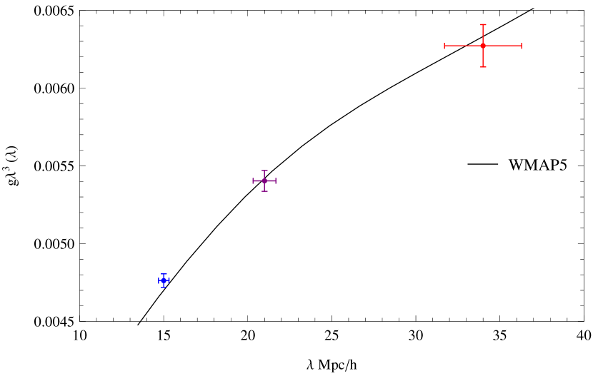
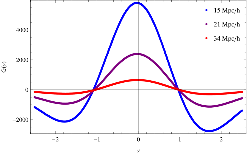
With 108 samples in hand, our fractional “uncertainty of the uncertainty” is $1/\sqrt{2(N-1)}=6.8\%$. It is notable that the systematic effect for the $21~{}h^{-1}$Mpc sample was very small, $-0.84$%, and that the $\chi^{2}$ best-fit genus amplitudes modeled the $g\lambda^{3}$ curve extraordinarily well (Fig. 3).

7. Discussion

With these results in hand, it is important to continue refining topological study of the SDSS LRG sample with $N$-body simulations. Extremely large cubes like HR3 allow for tight description of the cosmic variance in genus per unit volume $g$ and smoothing length $\lambda$. This statistical knowledge translates directly to the measurement of cosmological parameters such as $w$. A possible extension of this work is to more accurately model the SDSS survey with 108 less “ideal” masks. Another possible extension is to measure the variance in genus per cubic smoothing length $g\lambda^{3}$ for a large number of $\lambda$’s, perhaps iterating from $15~{}h^{-1}{\rm Mpc}$ to $34~{}h^{-1}{\rm Mpc}$ in small increments $\Delta\lambda<0.2~{}h^{-1}{\rm Mpc}$. Smooth plots of $\sigma_{g\lambda^{3}}$ and $\lambda-\lambda_{\rm true}$ as a function of $\lambda$ could yield useful information about the evolution of random and systematic error with scale.

Appendix A 3D Graphics of the Horizon Run 3

Figure 4.— Stereo View of the Horizon Run 3 spherical mock survey out to redshift $z=0.7$. In order to see this figure in 3D, cross you eyes until you see three purple sponges. Fuse the middle sponge and bring it into focus. The middle sponge should be in 3D.

Figure 5.— A red blue anaglyph of a spherical Horizon Run 3 Mock survey out to redshift $z=0.7$. The PSB subhalo counts have been smoothed with a Gaussian smoothing ball of $\lambda=34~{}h^{-1}\rm{Mpc}$. Requires red-cyan lensed glasses to view.

References

- Albrecht & Steinhardt (1982) Albrecht H. & Steinhardt P. J. 1982, Phys. Rev. Lett. 48, 1220
- Anderson et al. (2012) Anderson, et al. 2012, MNRAS, 427, 3435
- Choi et al. (2010) Choi, Y.-Y, Park, C., Kim, J., Gott, J.R., Weinberg, D.H., Vogeley, M.S., Kim, S.S. 2010, ApJS, 190, 181
- Eisenstein, et al. (2001) Eisenstein, D.J., Annis, J., Gunn, J.E., et al. 2001, AJ, 122, 2267
- Eisenstein et al. (2011) Eisenstein, D.J., Weinberg, D.H., et al. 2011, AJ, 142, 72
- Gott, Melott, & Dickinson (1986) Gott, J. R., Melott, A. L., & Dickinson, M. 1986, ApJ, 306, 341
- Gott, Weinberg, & Melott (1987) Gott, J. R., Weinberg, D.N., & Melott, A.L. 1987, ApJ, 319, 1
- Gott et al. (1989) Gott, J.R., et al. 1989, ApJ, 340, 625
- Gott et al. (2008) Gott, J. R., et al. 2008, ApJ, 675, 16
- Gott et al. (2009) Gott, J.R., et al. 2009, ApJ, 695, L45
- Guth (1981) Guth, A.H. 1981, Phys. Rev. D, 23, 347
- Hamilton, Gott, and Weinberg (1986) Hamilton, A. J. S., Gott, J. R., & Weinberg, D. W. 1986, ApJ, 309, 1
- Hikage et al. (2002) Hikage, C., et al. (The SDSS Collaboration) 2002, PASJ, 54, 707
- Hikage et al. (2003) Hikage, C., et al. 2003, PASJ, 55, 911
- Hinshaw et al. (2013) Hinshaw, G., Larson, D., Komatsu, E., et al. 2013, arXiv1212.5226
- Hogg (1999) Hogg, D. W. 1999 arXiv:astro-ph/9905116
- Kim & Park (2006) Kim, J., & Park, C. 2006, ApJ, 639, 600
- Kim et al. (2011) Kim, J., Park, C., Ross, G., Lee, S.M., & Gott, J.R. 2011, JKAS, 44. 217
- Komatsu et al. (2011) Komatsu, E., Smith, K.M., & Dunkley, J., et al. 2011, ApJS, 192, 18
- Linde (1982) Linde, A.D. 1982, Phys. Lett. B, 108, 389
- Linde (1983) Linde, A.D. 1983, Phys. Lett. B, 129, 177
- Lewis & Bridle (2002) Lewis, A., Bridle, S., 2002, Phys. Rev., D66 103511
- Matsubara (1994) Matsubara, T. 1994, ApJ, 434, L43
- Park & Gott (1991) Park, C., & Gott, J.R. 1991, ApJ, 378, 457
- Park, Gott, & da Costa (1992) Park, C., Gott, J.R., & da Costa, L.N. 1992, ApJ, 392, L51]
- Park et al. (1998) Park, C., Colley, W.N., Gott, J.R., Ratra, B., Spergel, D.N., & Sugiyama, N. 1998, ApJ, 506, 473
- Park, et al. (2005a) Park, C., Kim, J., & Gott, J.R. 2005a, ApJ, 633, 1
- Park et al. (2005b) Park, C., et al. (The SDSS Collaboration) 2005b, ApJ, 633, 11
- Park & Kim (2010) Park, C., & Kim, Y.-R. 2010, ApJ, 715, L185
- Park et al. (2012) Park, C., Choi, Y.-Y., Kim, J., Gott, J.R., Kim, S.S., & Kim, K.-S. 2012, ApJ, 759, L7
- Park et al. (2013) Park, C., Pranav, P., Chingangbam, P., van de Weygaert, R., Jones, B., Vegter, G., Kim, I., Hidding, J. & Hellwing, W.A. 2013, JKAS, 46, 125
- Press & Schechter (1974) Press, W.H., & Schechter, P. 1974, ApJ, 187, 425
- Slepian, Gott, & Zinn (2013) Slepian, Z., Gott, J.R., & Zinn, J. 2013, arXiv1301.4611
- Soneira & Peebles (1978) Soneira, R.M. and Peebles, P. J. E. 1978, A.J., 83, 845
- Spergel et al. (2003) Spergel, D.N., et al. 2003, ApJS, 148, 175
- Springel et al. (2005) Springel, V. 2005, Nature, 435, 629
- Strauss et al. (2002) Strauss, M.A., et al. 2002, AJ, 124, 1810
- Vogeley et al. (1994) Vogeley, M.S., Park, C., Geller, M.J., Huchra, J.P., & Gott, J.R. 1994, ApJ, 420, 525
- Weinberg (1988) Weinberg, D. H. 1988, PASP, 100, 1373
- Zunckel, Gott, & Lunnan (2011) Zunckel, C., Gott, J.R., & Lunnan, R. 2011, MNRAS, 412, 1401