An Online Algorithm for Separating Sparse and Low-dimensional Signal Sequences from their Sum
Abstract
This paper designs and extensively evaluates an online algorithm, called practical recursive projected compressive sensing (Prac-ReProCS), for recovering a time sequence of sparse vectors and a time sequence of dense vectors from their sum, , when the ’s lie in a slowly changing low-dimensional subspace of the full space. A key application where this problem occurs is in real-time video layering where the goal is to separate a video sequence into a slowly changing background sequence and a sparse foreground sequence that consists of one or more moving regions/objects on-the-fly. Prac-ReProCS is a practical modification of its theoretical counterpart which was analyzed in our recent work. Experimental comparisons demonstrating the advantage of the approach for both simulated and real videos, over existing batch and recursive methods, are shown. Extension to the undersampled case is also developed.
I Introduction
This paper designs and evaluates a practical algorithm for recovering a time sequence of sparse vectors and a time sequence of dense vectors from their sum, , when the ’s lie in a slowly changing low-dimensional subspace of . The magnitude of the entries of could be larger, roughly equal or smaller than that of the nonzero entries of . The extension to the undersampled case, , is also developed. The above problem can be interpreted as one of online/recursive sparse recovery from potentially large but structured noise. In this case, is the quantity of interest and is the potentially large but structured low-dimensional noise. Alternatively it can be posed as a recursive / online robust principal components analysis (PCA) problem. In this case , or in fact, the subspace in which it lies, is the quantity of interest while is the outlier.
A key application where the above problem occurs is in video layering where the goal is to separate a slowly changing background from moving foreground objects/regions [4, 5]. The foreground layer, e.g. moving people/objects, is of interest in applications such as automatic video surveillance, tracking moving objects, or video conferencing. The background sequence is of interest in applications such as background editing (video editing applications). In most static camera videos, the background images do not change much over time and hence the background image sequence is well modeled as lying in a fixed or slowly-changing low-dimensional subspace of [6, 5]. Moreover the changes are typically global, e.g. due to lighting variations, and hence modeling it as a dense image sequence is valid too [5]. The foreground layer usually consists of one or more moving objects/persons/regions that move in a correlated fashion, i.e. it is a sparse image sequence that often changes in a correlated fashion over time. Other applications where the above problem occurs include solving the video layering problem from compressive video measurements, e.g. those acquired using a single-pixel camera; online detection of brain activation patterns from full or undersampled functional MRI (fMRI) sequences (the “active” part of the brain forms the sparse image, while the rest of the brain which does not change much over time forms the low-dimensional part); or sensor networks based detection and tracking of abnormal events such as forest fires or oil spills. The single pixel imaging and undersampled fMRI applications are examples of the compressive case, with .
Related Work. Most high dimensional data often approximately lie in a lower dimensional subspace. Principal components’ analysis (PCA) is a widely used dimension reduction technique that finds a small number of orthogonal basis vectors (principal components), along which most of the variability of the dataset lies. For a given dimension, , PCA finds the -dimensional subspace that minimizes the mean squared error between data vectors and their projections into this subspace [7]. It is well known that PCA is very sensitive to outliers. Computing the PCs in the presence of outliers is called robust PCA. Solving the robust PCA problem recursively as more data comes in is referred to as online or recursive robust PCA. “Outlier” is a loosely defined term that usually refers to any corruption that is not small compared to the true signal (or data vector) and that occurs only occasionally. As suggested in [8], an outlier can be nicely modeled as a sparse vector.
In the last few decades, there has been a large amount of work on robust PCA, e.g. [4, 9, 10, 11, 12], and recursive robust PCA e.g. [13, 14, 15]. In most of these works, either the locations of the missing/corruped data points are assumed known [13] (not a practical assumption); or they first detect the corrupted data points and then replace their values using nearby values [14]; or weight each data point in proportion to its reliability (thus soft-detecting and down-weighting the likely outliers) [4, 15]; or just remove the entire outlier vector [11, 12]. Detecting or soft-detecting outliers () as in [14, 4, 15] is easy when the outlier magnitude is large, but not when it is of the same order or smaller than that of the ’s.
In a series of recent works [5, 16], a new and elegant solution to robust PCA called Principal Components’ Pursuit (PCP) has been proposed, that does not require a two step outlier location detection/correction process and also does not throw out the entire vector. It redefines batch robust PCA as a problem of separating a low rank matrix, , from a sparse matrix, , using the measurement matrix, . Other recent works that also study batch algorithms for recovering a sparse and a low-rank from or from undersampled measurements include [17, 18, 19, 20, 21, 22, 23, 24, 25, 26]. It was shown in [5] that by solving PCP:
| (1) |
one can recover and exactly, provided that (a) is “dense”; (b) any element of the matrix is nonzero w.p. , and zero w.p. , independent of all others (in particular, this means that the support sets of the different ’s are independent over time); and (c) the rank of and the support size of are small enough. Here is the nuclear norm of a matrix (sum of singular values of ) while is the norm of seen as a long vector.
Notice that most applications described above require an online solution. A batch solution would need a long delay; and would also be much slower and more memory-intensive than a recursive solution. Moreover, the assumption that the foreground support is independent over time is not usually valid. To address these issues, in the conference versions of this work [1, 2], we introduced a novel recursive solution called Recursive Projected Compressive Sensing (ReProCS). In recent work [27, 28, 29], we have obtained performance guarantees for ReProCS. Under mild assumptions (denseness, slow enough subspace change of and “some” support change at least every frames of ), we showed that, with high probability (w.h.p.), ReProCS can exactly recover the support set of at all times; and the reconstruction errors of both and are upper bounded by a time invariant and small value. The work of [27, 28] contains a partial result while [29] is a complete correctness result.
Contributions. The contributions of this work are as follows. (1) We design a practically usable modification of the ReProCS algorithm studied in [27, 28, 29]. By “practically usable”, we mean that (a) it requires fewer parameters and we develop simple heuristics to set these parameters without any model knowledge; (b) it exploits practically motivated assumptions and we demonstrate that these assumptions are valid for real video data. While denseness and gradual support change are also used in earlier works - [5, 16] and [30] respectively - slow subspace change is the key new (and valid) assumption introduced in ReProCS. (2) We show via extensive simulation and real video experiments that practical-ReProCS is more robust to correlated support change of than PCP and other existing work. Also, it is also able to recover small magnitude sparse vectors significantly better than other existing recursive as well as batch algorithms. (3) We also develop a compressive practical-ReProCS algorithm that can recover from . In this case and can be fat, square or tall.
More Related Work. Other very recent work on recursive / online robust PCA includes [31, 32, 33, 34, 35].
Some other related work includes work that uses structured sparsity models, e.g. [36]. For our problem, if it is known that the sparse vector consists of one or a few connected regions, these ideas could be incorporated into our algorithm as well. On the other hand, the advantage of the current approach that only uses sparsity is that it works both for the case of a few connected regions as well as for the case of multiple small sized moving objects, e.g. see the airport video results at http://www.ece.iastate.edu/~chenlu/ReProCS/Video_ReProCS.htm.
Paper Organization. We give the precise problem definition and assumptions in Sec II. The practical ReProCS algorithm is developed in Sec III. The algorithm for the compressive measurements’ case is developed in Sec IV. In Sec V, we demonstrate using real videos that the key assumptions used by our algorithm are true in practice. Experimental comparisons on simulated and real data are shown in Sec VI. Conclusions and future work are discussed in Sec VII.
I-A Notation
For a set , we use to denote its cardinality; and we use to denote its complement, i.e. . The symbols denote set union set intersection and set difference respectively (recall ). For a vector , denotes the th entry of and denotes a vector consisting of the entries of indexed by . We use to denote the norm of . The support of , , is the set of indices at which is nonzero, . We say that is s-sparse if .
For a matrix , denotes its transpose, and denotes its pseudo-inverse. For a matrix with linearly independent columns, . The notation denotes an empty matrix. We use to denote an identity matrix. For an matrix and an index set , is the sub-matrix of containing columns with indices in the set . Notice that . We use to denote . Given another matrix of size , constructs a new matrix by concatenating matrices and in horizontal direction. Thus, . We use the notation to denote the singular value decomposition (SVD) of with the diagonal entries of being arranged in non-decreasing order.
The interval notation and similarly the matrix
Definition I.1
The -restricted isometry constant (RIC) [37], , for an matrix is the smallest real number satisfying for all sets with and all real vectors of length .
Definition I.2
For a matrix ,
-
•
denotes the subspace spanned by the columns of .
-
•
is a basis matrix if .
-
•
The notation , or for short, means that is a basis matrix for i.e. satisfies and .
Definition I.3
-
•
The left singular values’ set of a matrix is the smallest set of indices of its singular values that contains at least of the total singular values’ energy. In other words, if , it is the smallest set such that .
-
•
The corresponding matrix of left singular vectors, , is referred to as the left singular vectors’ matrix.
-
•
The notation means that is the left singular vectors’ matrix for and is the diagonal matrix with diagonal entries equal to the b% left singular values’ set.
-
•
The notation means that contains the left singular vectors of corresponding to its largest singular values. This also sometimes referred to as: contains the top singular vectors of .
II Problem Definition and Assumptions
The measurement vector at time , , is an dimensional vector which can be decomposed as
| (2) |
Let denote the support set of , i.e.,
We assume that and satisfy the assumptions given below in the next three subsections. Suppose that an initial training sequence which does not contain the sparse components is available, i.e. we are given with . This is used to get an initial estimate of the subspace in which the ’s lie 111If an initial sequence without ’s is not available, one can use a batch robust PCA algorithm to get the initial subspace estimate as long as the initial sequence satisfies its required assumptions.. At each , the goal is to recursively estimate and and the subspace in which lies. By “recursively” we mean: use and the previous subspace estimate to estimate and .
The magnitude of the entries of may be small, of the same order, or large compared to that of the nonzero entries of . In applications where is the signal of interest, the case when is of the same order or larger than is the difficult case.
A key application where the above problem occurs is in separating a video sequence into background and foreground layers. Let denote the image at time , denote the foreground image at and the background image at , all arranged as 1-D vectors. Then, the image sequence satisfies
| (5) |
In fMRI, is the sparse active region image while is the background brain image. In both cases, it is fair to assume that an initial background-only training sequence is available. For video this means there are no moving objects/regions in the foreground. For fMRI, this means some frames are captured without providing any stimulus to the subject.
Let denote the empirical mean of the training background images. If we let , , , and
then, clearly, . Once we get the estimates , , we can also recover the foreground and background as
II-A Slowly changing low-dimensional subspace change
We assume that for large enough, any length subsequence of the ’s lies in a subspace of of dimension less than , and usually much less than . In other words, for large enough, . Also, this subspace is either fixed or changes slowly over time.
One way to model this is as follows [27]. Let where is an basis matrix with that is piecewise constant with time, i.e. for all and changes as
where and are basis matrices of size and respectively with and is a rotation matrix. Moreover, (a) ; (b) ; (c) ; and (d) there are a total of change times with .
Clearly, (a) implies that and (d) implies that . This, along with (b) and (c), helps to ensure that for any , , and for , 222 To address a reviewer comment, we explain this in detail here. Notice first that (c) implies that . Also, (b) implies that . First consider the case when both and lie in . In this case, for any . Thus for any , . Next consider the case when and . In this case, . Thus, for any , . Finally consider the case when and for a . In this case, can be rewritten as with and . Clearly, . Moreover, . Thus, in this case again for any , . .
By slow subspace change, we mean that: for , is initially small and increases gradually. In particular, we assume that, for ,
and increases gradually after . One model for “increases gradually” is as given in [27, Sec III-B]. Nothing in this paper requires the specific model and hence we do not repeat it here.
The above piecewise constant subspace change model is a simplified model for what typically happens in practice. In most cases, changes a little at each in such a way that the low-dimensional assumption approximately holds. If we try to model this, it would result in a nonstationary model that is difficult to precisely define or to verify (it would require multiple video sequences of the same type to verify) 333With letting be a zero mean random variable with a covariance matrix that is constant for sub-intervals within , the above model is a piecewise wide sense stationary approximation to the nonstationary model..
Since background images typically change only a little over time (except in case of a camera viewpoint change or a scene change), it is valid to model the mean-subtracted background image sequence as lying in a slowly changing low-dimensional subspace. We verify this assumption in Sec V.
II-B Denseness
To state the denseness assumption, we first need to define the denseness coefficient. This is a simplification of the one introduced in our earlier work [27].
Definition II.1 (denseness coefficient)
For a matrix or a vector , define
| (6) |
where is the vector or matrix -norm. Recall that is short for . Similarly is short for . Notice that is a property of the subspace . Note also that is a non-decreasing function of and of .
We assume that the subspace spanned by the ’s is dense, i.e.
for a significantly smaller than one. Moreover, a similar assumption holds for with a tighter bound: . This assumption is similar to one of the denseness assumptions used in [38, 5]. In [5], a bound is assumed on and where and are the matrices containing the left and right singular vectors of the entire matrix, ; and a tighter bound is assumed on . In our notation, .
The following lemma, proved in [27], relates the RIC of , when is a basis matrix, to the denseness coefficient for . Notice that is an matrix that has rank and so it cannot be inverted.
Lemma II.2
For a basis matrix, ,
Thus, the denseness assumption implies that the RIC of the matrix is small. Using any of the RIC based sparse recovery results, e.g. [39], this ensures that for , -sparse vectors are recoverable from by minimization.
Very often, the background images primarily change due to lighting changes (in case of indoor sequences) or due to moving waters or moving leaves (in case of many outdoor sequences) [5, 27]. All of these result in global changes and hence it is valid to assume that the subspace spanned by the background image sequences is dense.
II-C Small support size, some support change, small support change assumption on
Let the sets of support additions and removals be
(1) We assume that
In particular, this implies that we either need and ( is sparse with support size at most , and its support changes slowly) or, in cases when the change is large, we need (need a tighter bound on the support size).
(2) We also assume that there is some support change every few frames, i.e. at least once every frames, . Practically, this is needed to ensure that at least some of the background behind the foreground is visible so that the changes to the background subspace can be estimated.
In the video application, foreground images typically consist of one or more moving objects/people/regions and hence are sparse. Also, typically the objects are not static, i.e. there is some support change at least every few frames. On the other hand, since the objects usually do not move very fast, slow support change is also valid most of the time. The time when the support change is almost comparable to the support size is usually when the object is entering or leaving the image, but these are the exactly the times when the object’s support size is itself small (being smaller than is a valid). We show some verification of these assumptions in Sec V.
III Prac-ReProCS: Practical ReProCS
We first develop a practical algorithm based on the basic ReProCS idea from our earlier work [27]. Then we discuss how the sparse recovery and support estimation steps can be improved. The complete algorithm is summarized in Algorithm 1. Finally we discuss an alternate subspace update procedure in Sec III-D.
III-A Basic algorithm
We use to denote estimates of , its support, , and respectively; and we use to denote the basis matrix for the estimated subspace of at time . Also, let
| (7) |
Given the initial training sequence which does not contain the sparse components, we compute as an approximate basis for , i.e. . Let . We need to compute an approximate basis because for real data, the ’s are only approximately low-dimensional. We use or depending on whether the low-rank part is approximately low-rank or almost exactly low-rank. After this, at each time , ReProCS involves 4 steps: (a) Perpendicular Projection; (b) Sparse Recovery (recover and ); (c) Recover ; (d) Subspace Update (update ).
Perpendicular Projection. In the first step, at time , we project the measurement vector, , into the space orthogonal to to get the projected measurement vector,
| (8) |
Sparse Recovery (Recover and ). With the above projection, can be rewritten as
| (9) |
Because of the slow subspace change assumption, projecting orthogonal to nullifies most of the contribution of and hence can be interpreted as small “noise”. We explain this in detail in Appendix -A.
Thus, the problem of recovering from becomes a traditional noisy sparse recovery / CS problem. Notice that, since the projection matrix, , has rank , therefore has only this many “effective” measurements, even though its length is . To recover from , one can use minimization [40, 39], or any of the greedy or iterative thresholding algorithms from literature. In this work we use minimization: we solve
| (10) |
and denote its solution by . By the denseness assumption, is dense. Since approximates it, this is true for as well [27, Lemma 6.6]. Thus, by Lemma II.2, the RIC of is small enough. Using [39, Theorem 1], this and the fact that is small ensures that can be accurately recovered from . The constraint used in the minimization should equal or its upper bound. Since is unknown we set where .
By thresholding on to get an estimate of its support followed by computing a least squares (LS) estimate of on the estimated support and setting it to zero everywhere else, we can get a more accurate estimate, , as suggested in [41]. We discuss better support estimation and its parameter setting in Sec III-C.
Recover . The estimate is used to estimate as . Thus, if is recovered accurately, so will .
Subspace Update (Update ). Within a short delay after every subspace change time, one needs to update the subspace estimate, . To do this in a provably reliable fashion, we introduced the projection PCA (p-PCA) algorithm in [27]. The algorithm studied there used knowledge of the subspace change times and of the number of new directions . Let denote the final estimate of a basis for the span of . It is assumed that the delay between change times is large enough so that is an accurate estimate. At , p-PCA gets the first estimate of the new directions, , by projecting the last ’s perpendicular to followed by computing the top left singular vectors of the projected data matrix. It then updates the subspace estimate as . The same procedure is repeated at every for and each time we update the subspace as . Here is chosen so that the subspace estimation error decays down to a small enough value within p-PCA steps.
In this paper, we design a practical version of p-PCA which does not need knowledge of or . This is summarized in Algorithm 1. The key idea is as follows. We let be the largest singular value of the training dataset. This serves as the noise threshold for approximately low rank data. We split projection PCA into two phases: “detect subspace change” and “p-PCA”. We are in the detect phase when the previous subspace has been accurately estimated. Denote the basis matrix for this subspace by . We detect the subspace change as follows. Every frames, we project the last ’s perpendicular to and compute the SVD of the resulting matrix. If there are any singular values above , this means that the subspace has changed. At this point, we enter the “p-PCA” phase. In this phase, we repeat the p-PCA steps described above with the following change: we estimate as the number of singular values above , but clipped at (i.e. if the number is more than then we clip it to ). We stop either when the stopping criterion given in step 4(b)iv is achieved ( and the projection of along is not too different from that along ) or when .
For the above algorithm, with theoretically motivated choices of algorithm parameters, under the assumptions from Sec II, it is possible to show that, w.h.p., the support of is exactly recovered, the subspace of ’s is accurately recovered within a finite delay of the change time. We provide a brief overview of the proof from [27, 29] in Appendix -A that helps explain why the above approach works.
Remark III.1
The p-PCA algorithm only allows addition of new directions. If the goal is to estimate the span of , then this is what is needed. If the goal is sparse recovery, then one can get a smaller rank estimate of by also including a step to delete the span of the removed directions, . This will result in more “effective” measurements available for the sparse recovery step and hence possibly in improved performance. The simplest way to do this is to do one simple PCA step every some frames. In our experiments, this did not help much though. A provably accurate solution is described in [27, Sec VII].
Remark III.2
The p-PCA algorithm works on small batches of frames. This can be made fully recursive if we compute the SVD of using the incremental SVD (inc-SVD) procedure summarized in Algorithm 2 [13] for one frame at a time. As explained in [13] and references therein, we can get the left singular vectors and singular values of any matrix recursively by starting with and calling [, ] = inc-SVD(, , ) for every column or for short batches of columns of size of . Since we use which is a small value, the use of incremental SVD does not speed up the algorithm in practice and hence we do not report results using it.
Input: ; Output: , , ; Parameters: . We used in all experiments ( needs to only be large compared to ); we used for approximately low-rank data (all real videos and the lake video with simulated foreground) and used for almost exactly low rank data (simulated data); we used whenever was of the same order or larger than (all real videos and the lake video) and used when it was much smaller (simulated data with small magnitude ).
Initialization
-
•
.
-
•
Set , , ,
-
•
Initialize and .
For do
-
1.
Perpendicular Projection: compute with
- 2.
-
3.
Estimate :
-
4.
Update : projection PCA
-
(a)
If and , (here is the remainder when is divided by )
-
i.
compute the SVD of and check if any singular values are above
-
ii.
if the above number is more than zero then set , increment , set , reset
Else .
-
i.
-
(b)
If and ,
-
i.
compute the SVD of ,
-
ii.
let retain all its left singular vectors with singular values above or all top left singular vectors whichever is smaller,
-
iii.
update , increment
-
iv.
If and for ; or ,
then , and reset .
Else .
-
i.
-
(a)
III-B Exploiting slow support change when valid
In [27, 28], we always used minimization followed by thresholding and LS for sparse recovery. However if slow support change holds, one can replace simple minimization by modified-CS [30] which requires fewer measurements for exact/accurate recovery as long as the previous support estimate, , is an accurate enough predictor of the current support, . In our application, is likely to contain a significant number of extras and in this case, a better idea is to solve the following weighted problem [42, 43]
| (11) |
with (modified-CS solves the above with ). Denote its solution by . One way to pick is to let it be proportional to the estimate of the percentage of extras in . If slow support change does not hold, the previous support estimate is not a good predictor of the current support. In this case, doing the above is a bad idea and one should instead solve simple , i.e. solve (11) with . As explained in [43], if the support estimate contains at least correct entries, then weighted is better than simple . We use the above criteria with true values replaced by estimates. Thus, if , then we solve (11) with , else we solve it with .
III-C Improved support estimation
A simple way to estimate the support is by thresholding the solution of (11). This can be improved by using the Add-LS-Del procedure for support and signal value estimation [30]. We proceed as follows. First we compute the set by thresholding on in order to retain its largest magnitude entries. We then compute a LS estimate of on while setting it to zero everywhere else. As explained earlier, because of the LS step, is a less biased estimate of than . We let to allow for a small increase in the support size from to . A larger value of also makes it more likely that elements of the set are detected into the support estimate444Due to the larger weight on the term as compared to that on the term, the solution of (11) is biased towards zero on and thus the solution values along are smaller than the true ones..
The final estimate of the support, , is obtained by thresholding on using a threshold . If is appropriately chosen, this step helps to delete some of the extra elements from and this ensures that the size of does not keep increasing (unless the object’s size is increasing). An LS estimate computed on gives us the final estimate of , i.e. . We use except in situations where - in this case we use . An alternate approach is to let be proportional to the noise magnitude seen by the step, i.e. to let , however this approach required different values of for different experiments (it is not possible to specify one that works for all experiments).
The complete algorithm with all the above steps is summarized in Algorithm 1.
-
1.
set and
-
2.
compute QR decomposition of , i.e. (here is a basis matrix and is an upper triangular matrix)
-
3.
compute the SVD:
-
4.
update and
Note: As explained in [13], due to numerical errors, step 4 done too often can eventually result in no longer being a basis matrix. This typically occurs when one tries to use inc-SVD at every time , i.e. when is a column vector. This can be addressed using the modified Gram Schmidt re-orthonormalization procedure whenever loss of orthogonality is detected [13].
III-D Simplifying subspace update: simple recursive PCA
Even the practical version of p-PCA needs to set and besides also setting and . Thus, we also experiment with using PCA to replace p-PCA (it is difficult to prove a performance guarantee with PCA but that does not necessarily mean that the algorithm itself will not work). The simplest way to do this is to compute the top left singular vectors of either at each time or every frames. While this is simple, its complexity will keep increasing with time which is not desirable. Even if we use the last frames instead of all past frames, will still need to be large compared to to get an accurate estimate. To address this issue, we can use the recursive PCA (incremental SVD) algorithm given in Algorithm 2. We give the complete algorithm that uses this and a rank truncation step every frames (motivated by [13]) in Algorithm 3.
Input: ; Output: , , ; Parameters: , set in all experiments, set as explained in Algorithm 1.
Initialization: , , , initialize , , and . For do
IV Compressive Measurements: Recovering
Consider the problem of recovering from
when and are and matrices, is an length vector and is an length vector. In general can be larger, equal or smaller than or . In the compressive measurements’ case, . To specify the assumptions needed in this case, we need to define the basis matrix for and we need to define a generalization of the denseness coefficient.
Definition IV.1
Let and let .
Definition IV.2
For a matrix or a vector , define
| (12) |
where is the vector or matrix -norm. This quantifies the incoherence between the subspace spanned by any set of columns of and the range of .
We assume the following.
- 1.
-
2.
The matrix satisfies the restricted isometry property [39], i.e. .
-
3.
The denseness assumption is replaced by: , for a that is small compared to one. Notice that this depends on the ’s and on the matrices and .
Assume that we are given an initial training sequence that satisfies for . The goal is to recover at each time . It is not possible to recover unless is time-varying (this case is studied in [44]). In many imaging applications, e.g. undersampled fMRI or single-pixel video imaging, ( is a partial Fourier matrix for MRI and is a random Gaussian or Rademacher matrix for single-pixel imaging). On the other hand, if is large but low-dimensional sensor noise, then (identity matrix), while is the measurement matrix.
Let . It is easy to see that if lies in a slowly changing low-dimensional subspace, the same is also true for the sequence . Consider the problem of recovering from when an initial training sequence for is available. Using this sequence, it is possible to estimate its approximate basis as explained earlier. If we then project into the subspace orthogonal to , the resulting vector satisfies
where is small noise for the same reasons explained earlier. Thus, one can still recover from by or weighted minimization followed by support recovery and LS. Then, gets recovered as and this is used for updating its subspace estimate. We summarize the resulting algorithm in Algorithm 4. This is being analyzed in ongoing work [45].
The following lemma explains why some of the extra assumptions are needed for this case.
Lemma IV.3
[45] For a basis matrix, ,
Using the above lemma with , it is clear that incoherence of w.r.t. any set of columns of along with RIP of ensures that any sparse vector can be recovered from by minimization. In compressive ReProCS, the measurement matrix uses instead of and also involves small noise. With more work, these arguments can be extended to this case as well [see [45]].
V Model Verification
V-A Low-dimensional and slow subspace change assumption
We used two background image sequence datasets. The first was a video of lake water motion. For this sequence, and the number of images were 1500. The second was an indoor video of window curtains moving due to the wind. There was also some lighting variation. The latter part of this sequence also contains a foreground (various persons coming in, writing on the board and leaving). For this sequence, the image size was and the number of background-only images were 1755. Both sequences are posted at http://www.ece.iastate.edu/~hanguo/PracReProCS.html.
First note that any given background image sequence will never be exactly low-dimensional, but only be approximately so. Secondly, in practical data, the subspace does not just change as simply as in the model of Sec II-A. Typically there are some changes to the subspace at every time . Moreover, with just one training sequence of a given type, it is not possible to estimate the covariance matrix of at each and thus one cannot detect the subspace change times. The only thing one can do is to assume that there may be a change every frames, and that during these frames the ’s are stationary and ergodic; estimate the covariance matrix of for this period using a time average; compute its eigenvectors corresponding to energy (or equivalently compute the approximate basis of ) and use these as . These can be used to test our assumptions.
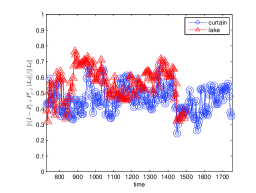
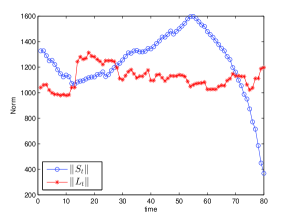
Testing for slow subspace change can be done in various ways. In [27, Fig 6], we do this after low-rankifying the video data first. This helps to very clearly demonstrate slow subspace change, but then it is not checking what we really do on real video data. In this work, we proceed without low-rankifying the data. We let and with . Let denote the mean subtracted background image sequence, i.e. where . We computed as . We observed that for curtain sequence, while for lake sequence. In other words, 95% of the energy is contained in only 38 or lesser directions in either case, i.e. both sequences are approximately low-dimensional. Notice that the dimension of the matrix is and is much larger than 38. To test for slow subspace change, in Fig. 1(a), we plot when . Notice that, after every change time (), this quantity is initially small for the first 100-150 frames and then increases gradually. It later decreases also but that is allowed (all we need is that it be small initially and increase slowly).
V-B Denseness assumption
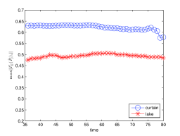
Exactly verifying the denseness assumption is impossible since computing has exponential complexity (one needs to check all sets of size ). Instead, to get some idea if it holds even just for replaced by , in Fig. 1(b), we plot where is the true or estimated support of at time . For the lake sequence, is simulated and hence known. For the curtain sequence, we select a part of the sequence in which the person is wearing a black shirt (against a white curtains’ background). This part corresponds to to . For this part, ReProCS returns a very accurate estimate of , and we use this estimated support as a proxy for the true support .
V-C Support size, support change and slow support change
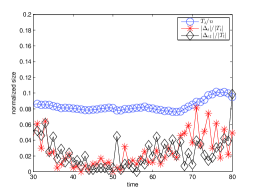
For real video sequences, it is not possible to get the true foreground support. Thus we used for the part of the curtain sequence described above in Sec V-B as a proxy for . We plot the support size normalized by the image size , and we plot the number of additions and removals normalized by the support size, i.e. and in Fig. 1(c). Notice from the figure that the support size is at most 10.2% of the image size. Notice also that at least at every 3 frames, there is at least a 1% support change. Thus there is some support change every few frames, thus exposing the part of the background behind the foreground. Finally notice that the maximum number of support changes is only 9.9% of the support size, i.e. slow support change holds for this piece.
VI Simulation and Experimental Results
In this section, we show comparisons of ReProCS with other batch and recursive algorithms for robust PCA. For implementing the or weighted minimizations, we used the YALL1 minimization toolbox [46], its code is available at http://yall1.blogs.rice.edu/.
Code and data for our algorithms and for all experiments given below is available at http://www.ece.iastate.edu/~hanguo/ReProCS_demo.rar.
Simulated Data. In this experiment, the measurement at time , , is an vector with . We generated using the autoregressive model described in [1] with auto-regression parameter 0.1, and the decay parameter . The covariance of a direction decayed to zero before being removed. There was one change time . For , was a rank matrix and was a diagonal matrix with entries . At , new directions, , got added with being diagonal with entries 60 and 50. Also, the variance along two existing directions started to decay to zero exponentially. We used and . The matrix was generated as the first 22 columns of an random orthonormal matrix (generated by first generating an matrix random Gaussian matrix and then orthonormalizing it). For , and hence . For , the support set, , was generated in a correlated fashion: contained one block of size 9 or 27 (small and large support size cases). The block stayed static with probability and move up or down by one pixel with probability each independently at each time. Thus the support sets were highly correlated. The magnitude of the nonzero elements of is fixed at either 100 (large) or 10 (small).
For the small magnitude case, ranged from 150 to 250 while was equal to 30 and 52, i.e. in this case . For the large magnitude case, was 300 and 520. We implemented ReProCS (Algorithm 1) with since this data is exactly low-rank. We used for the small magnitude case and for the other case. We compared with three recursive robust PCA methods – incremental robust subspace learning (iRSL) [15] and adapted (outlier-detection enabled) incremental SVD (adapted-iSVD) [13] and GRASTA [31] – and with two batch methods – Principal Components’ Pursuit (PCP) [5] 555We use the Accelerated Proximal Gradient algorithm[47] and Inexact ALM algorithm [48] (designed for large scale problems) to solve PCP (1). The code is available at http://perception.csl.uiuc.edu/matrix-rank/sample_code.html. and robust subspace learning (RSL)666The code of RSL is available at http://www.salleurl.edu/ftorre/papers/rpca/rpca.zip. [4]. Results are shown in Table I.
From these experiments, we can conclude that ReProCS is able to successfully recover both small magnitude and fairly large support-sized ’s; iRSL has very bad performance in both cases; RSL, PCP and GRASTA work to some extent in certain cases, though not as well as ReProCS. ReProCS operates by first approximately nullifying , i.e. computing as in (8), and then recovering by exploiting its sparsity. iRSL and RSL also compute the same way, but they directly use to detect or soft-detect (and down-weight) the support of by thresholding. Recall that can be rewritten as . As the support size of increases, the interference due to becomes larger, resulting in wrong estimates of . For the same reason, direct thresholding is also difficult when some entries of are small while others are not. Adapted-iSVD is our adaptation of iSVD [13] in which we use the approach of iRSL described above to provide the outlier locations to iSVD (iSVD is an algorithm for recursive PCA with missing entries or what can be called recursive low-rank matrix completion). It fills in the corrupted locations of by imposing that lies in . We used a threshold of for both iRSL and adapted-iSVD (we also tried various other options for thresholds but with similar results). Since adapted-iSVD and iRSL are recursive methods, a wrong , in turn, results in wrong subspace updates, thus also causing to become large and finally causing the error to blow up.
RSL works to some extent for larger support size of ’s but fails when the magnitude of the nonzero ’s is small. PCP fails since the support sets are generated in a highly correlated fashion and the support sizes are large (resulting in the matrix being quite rank deficient also). GRASTA [31] is a recent recursive method from 2012. It was implemented using code posted at https://sites.google.com/site/hejunzz/grasta. We tried two versions of GRASTA: the demo code as it is and the demo code modified so that it used as much information as ReProCS used (i.e. we used all available frames for training instead of just 100; we used all measurements instead of just 20% randomly selected pixels; and we used returned by ReProCS as the rank input instead of using rank=5 always). In this paper, we show the latter case. Both experiments are shown on our supplementary material page http://www.ece.iastate.edu/~hanguo/PracReProCS.html.
Partly Simulated Video: Lake video with simulated foreground. In the comparisons shown next, we only compare with PCP, RSL and GRASTA. To address a reviewer comment, we also compare with the batch algorithm of [34, 35] (referred to as MG in the figures) implemented using code provided by the authors. There was not enough information in the papers or in the code to successfully implement the recursive algorithm.
We implemented ReProCS (Algorithm 1 and Algorithm 3) with since the videos are only approximately low-rank and we used since the magnitude of is not small compared to that of . The performance of both ReProCS-pPCA (Algorithm 1) and ReProCS-recursive-PCA (Algorithm 3) was very similar. Results with using the latter are shown in Fig. 6.
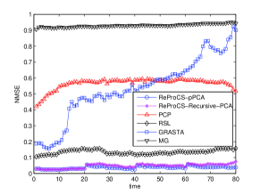
We used the lake sequence described earlier to serve as a real background sequence. Foreground consisting of a rectangular moving object was overlaid on top of it using (5). The use of a real background sequence allows us to evaluate performance for data that only approximately satisfies the low-dimensional and slow subspace change assumptions. The use of the simulated foreground allows us to control its intensity so that the resulting is small or of the same order as (making it a difficult sequence), see Fig. 2(b).
The foreground was generated as follows. For , . For , consists of a moving block whose centroid moves horizontally according to a constant velocity model with small random acceleration [49, Example V.B.2]. To be precise, let be the horizontal location of the block’s centroid at time , let denote its horizontal velocity. Then satisfies where and is a zero mean truncated Gaussian with variance and with . The nonzero pixels’ intensity is i.i.d. over time and space and distributed as , i.e. for . In our experiments, we generated the data with , , , , and . With these values of , as can be seen from Fig. 2(b), is roughly equal or smaller than making it a difficult sequence. Since it is not much smaller, ReProCS used ; since background data is approximately low-rank it used .
We generated 50 realizations of the video sequence using these parameters and compared all the algorithms to estimate , and then the foreground and the background sequences. We show comparisons of the normalized mean squared error (NMSE) in recovering in Fig. 2(a). Visual comparisons of both foreground and background recovery for one realization are shown in Fig. 3. The recovered foreground image is shown as a white-black image showing the foreground support: pixels in the support estimate are white. PCP gives large error for this sequence since the object moves in a highly correlated fashion and occupies a large part of the image. GRASTA also does not work. RSL is able to recover a large part of the object correctly, however it also recovers many more extras than ReProCS. The reason is that the magnitude of the nonzero entries of is quite small (recall that for ) and is such that is about as large as or sometimes larger (see Fig. 2(b)).
Real Video Sequences. Next we show comparisons on two real video sequences. These are originally taken from http://perception.i2r.a-star.edu.sg/bk_model/bk_index.html and http://research.microsoft.com/en-us/um/people/jckrumm/wallflower/testimages.htm, respectively. The first is the curtain sequence described earlier. For , in the foreground, a person with a black shirt walks in, writes on the board and then walk out, then a second person with a white shirt does the same and then a third person with a white shirt does the same. This video is challenging because (i) the white shirt color and the curtains’ color is quite similar, making the corresponding small in magnitude; and (ii) because the background variations are quite large while the foreground person moves slowly. As can be seen from Fig. 4, ReProCS’s performance is significantly better than that of the other algorithms for both foreground and background recovery. This is most easily seen from the recovered background images. One or more frames of the background recovered by PCP, RSL and GRASTA contains the person, while none of the ReProCS ones does.
The second sequence consists of a person entering a room containing a computer monitor that contains a white moving region. Background changes due to lighting variations and due to the computer monitor. The person moving in the foreground occupies a very large part of the image, so this is an example of a sequence in which the use of weighted is essential (the support size is too large for simple to work). As can be seen from Fig. 5, for most frames, ReProCS is able to recover the person correctly. However, for the last few frames which consist of the person in a white shirt in front of the white part of the screen, the resulting is too small even for ReProCS to correctly recover. The same is true for the other algorithms. Videos of all above experiments and of a few others are posted at http://www.ece.iastate.edu/~hanguo/PracReProCS.html.
Time Comparisons. The time comparisons are shown in Table II. In terms of speed, GRASTA is the fastest even though its performance is much worse. ReProCS is the second fastest. We expect that ReProCS can be speeded up by using mex files (C/C++ code) for the subspace update step. PCP and RSL are slower because they jointly process the entire image sequence. Moreover, ReProCS and GRASTA have the advantage of being recursive methods, i.e. the foreground/background recovery is available as soon as a new frame appears while PCP or RSL need to wait for the entire image sequence.
Compressive ReProCS: comparisons for simulated video. We compare compressive ReProCS with SpaRCS [20] which is a batch algorithm for undersampled robust PCA / separation of sparse and low-dimensional parts(its code is downloaded from http://www.ece.rice.edu/~aew2/sparcs.html). No code is available for most of the other compressive batch robust PCA algorithms such as [24, 25]. SpaRCS is a greedy approach that combines ideas from CoSaMP [50] for sparse recovery and ADMiRA [51] for matrix completion. The comparison is done for compressive measurements of the lake sequence with foreground simulated as explained earlier. The matrix is random Gaussian with . Recall that . The SpaRCS code required the background data rank and foreground sparsity as inputs. For rank, we used returned by ReProCS, for sparsity we used the true size of the simulated foreground. As can be seen from Fig. 7, SpaRCS does not work while compressive ReProCS is able to recover fairly accurately, though of course the errors are larger than in the full sampled case. All experiments shown in [20] are for very slow changing backgrounds and for foregrounds with very small support sizes, while neither is true for our data.
| (a) for and for | ||||||
| ReProCS-pPCA | RSL | PCP | GRASTA | adapted-iSVD | iRSL | |
| (b) for and for | ||||||
| ReProCS-pPCA | RSL | PCP | GRASTA | adapted-iSVD | iRSL | |
| DataSet | Image Size | Sequence Length | ReProCS-pPCA | ReProCS-Recursive-PCA | PCP | RSL | GRASTA |
|---|---|---|---|---|---|---|---|
| Lake | sec | sec | 245.03 sec | 213.36 sec | sec | ||
| Curtain | sec | sec | 1079.59 sec | 643.98 sec | sec | ||
| Person | sec | sec | 27.72 sec | 121.31 sec | sec |
|
|
|
|
|
|
| original ReProCS PCP RSL GRASTA MG ReProCS PCP RSL GRASTA MG |
| (fg) (fg) (fg) (fg) (fg) (bg) (bg) (bg) (bg) (bg) |
|
|
|
|
|
|
|
|
|
|
| original ReProCS PCP RSL GRASTA MG ReProCS PCP RSL GRASTA MG |
| (fg) (fg) (fg) (fg) (fg) (bg) (bg) (bg) (bg) (bg) |
|
|
|
|
|
|
| original ReProCS PCP RSL GRASTA MG ReProCS PCP RSL GRASTA MG |
| (fg) (fg) (fg) (fg) (fg) (bg) (bg) (bg) (bg) (bg) |
|
|
|
|
|
|
|
|
|
|
|
|
| original ReProCS SparCS |
VII Conclusions and Future Work
This work designed and evaluated Prac-ReProCS which is a practically usable modification of its theoretical counterpart that was studied in our earlier work [27, 28, 29]. We showed that Prac-ReProCS has excellent performance for both simulated data and for a real application (foreground-background separation in videos) and the performance is better than many of the state-of-the-art algorithms from recent work. Moreover, most of the assumptions used to obtain its guarantees are valid for real videos. Finally we also proposed and evaluated a compressive prac-ReProCS algorithm. In ongoing work, on one end, we are working on performance guarantees for compressive ReProCS [45] and on the other end, we are developing and evaluating a related approach for functional MRI. In fMRI, one is allowed to change the measurement matrix at each time. However if we replace by in Sec IV the compressive ReProCS algorithm does not apply because is not low-dimensional [44].
-A Detailed Discussion of Why ReProCS Works
Define the subspace estimation error as
where both and are basis matrices. Notice that this quantity is always between zero and one. It is equal to zero when contains and it is equal to one if for at least one column of .
Recall that for , . Thus, can be rewritten as
where and .
Let and . We explain here the key idea of why ReProCS works [27, 29]. Assume the following hold besides the assumptions of Sec II.
-
1.
Subspace change is detected immediately, i.e. and is known.
-
2.
Pick a . Assume that for a that satisfies . Since is very small, can be very large.
-
3.
Assume that for a as defined below.
-
4.
Assume the following model on the gradual increase of : for , for a and .
- 5.
-
6.
Assume that projection PCA is done times with chosen so that .
Assume that at , . We will argue below that . Since is small, this error is always small and bounded.
First consider a . At this time, . Thus,
| (13) | |||||
By construction, is very small and hence the second term in the bound is the dominant one. By the slow subspace assumption . Recall that is the “noise” seen by the sparse recovery step. The above shows that this noise is small compared to . Moreover, using Lemma II.2 and simple arguments [see [27, Lemma 6.6]], it can be shown that
is small. These two facts along with any RIP-based result for minimization, e.g. [39], ensure that is recovered accurately in this step. If the smallest nonzero entry of is large enough, it is possible get a support threshold that ensures exact support recovery. Then, the LS step gives a very accurate final estimate of and it allows us to get an exact expression for . Since , this means that is also recovered accurately and . This is then used to argue that p-PCA at “works”.
Next consider . At this time, . Then, it is easy to see that
| (14) | |||||
Ignoring the first term, in this interval, , i.e. the noise seen by the sparse recovery step decreases exponentially with every p-PCA step. This, along with a bound on (this bound needs a more complicated argument than that for , see [27, Lemma 6.6]), ensures that the recovery error of , and hence also of , decreases roughly exponentially with . This is then used to argue that the p-PCA error also decays roughly exponentially with .
Finally for , because of the choice of , we have that . At this time, we set . Thus, .
References
- [1] C. Qiu and N. Vaswani, “Real-time robust principal components’ pursuit,” in Allerton Conf. on Communications, Control and Computing, 2010.
- [2] C. Qiu and N. Vaswani, “Recursive sparse recovery in large but correlated noise,” in Allerton Conf. on Communication, Control, and Computing, 2011.
- [3] H. Guo, C. Qiu, and N. Vaswani, “Practical reprocs for separating sparse and low-dimensional signal sequences from their sum - part 1,” in IEEE Intl. Conf. Acoustics, Speech, Sig. Proc. (ICASSP), 2014.
- [4] F. De La Torre and M. J. Black, “A framework for robust subspace learning,” International Journal of Computer Vision, vol. 54, pp. 117–142, 2003.
- [5] E. J. Candès, X. Li, Y. Ma, and J. Wright, “Robust principal component analysis?,” Journal of ACM, vol. 58, no. 3, 2011.
- [6] J. Wright and Y. Ma, “Dense error correction via l1-minimization,” IEEE Trans. on Info. Th., vol. 56, no. 7, pp. 3540–3560, 2010.
- [7] Jolliffe I.T., Principal Component Analysis, Springer, second edition, 2002.
- [8] J. Wright and Y. Ma, “Dense error correction via l1-minimization,” IEEE Trans. Info. Th., vol. 56, no. 7, pp. 3540–3560, July 2010.
- [9] S. Roweis, “Em algorithms for pca and spca,” Advances in Neural Information Processing Systems, pp. 626–632, 1998.
- [10] T. Zhang and G. Lerman, “A novel m-estimator for robust pca,” arXiv:1112.4863v3, to appear in Journal of Machine Learning Research, 2013.
- [11] H. Xu, C. Caramanis, and S. Sanghavi, “Robust pca via outlier pursuit,” IEEE Tran. on Information Theory, vol. 58, no. 5, 2012.
- [12] Michael McCoy and Joel A Tropp, “Two proposals for robust pca using semidefinite programming,” Electronic Journal of Statistics, vol. 5, pp. 1123–1160, 2011.
- [13] M. Brand, “Incremental singular value decomposition of uncertain data with missing values,” in European Conference on Computer Vision, 2002, pp. 707–720.
- [14] D. Skocaj and A. Leonardis, “Weighted and robust incremental method for subspace learning,” in IEEE Intl. Conf. on Computer Vision (ICCV), Oct 2003, vol. 2, pp. 1494 –1501.
- [15] Y. Li, L. Xu, J. Morphett, and R. Jacobs, “An integrated algorithm of incremental and robust pca,” in IEEE Intl. Conf. Image Proc. (ICIP), 2003, pp. 245–248.
- [16] V. Chandrasekaran, S. Sanghavi, P. A. Parrilo, and A. S. Willsky, “Rank-sparsity incoherence for matrix decomposition,” SIAM Journal on Optimization, vol. 21, 2011.
- [17] Michael B McCoy and Joel A Tropp, “Sharp recovery bounds for convex deconvolution, with applications,” arXiv:1205.1580, accepted to J. Found. Comput. Math, 2012.
- [18] Venkat Chandrasekaran, Benjamin Recht, Pablo A. Parrilo, and Alan S. Willsky, “The convex geometry of linear inverse problems,” Foundations of Computational Mathematics, , no. 6, 2012.
- [19] Yue Hu, Sajan Goud, and Mathews Jacob, “A fast majorize-minimize algorithm for the recovery of sparse and low-rank matrices,” IEEE Transactions on Image Processing, vol. 21, no. 2, pp. 742=753, Feb 2012.
- [20] A. E. Waters, A. C. Sankaranarayanan, and R. G. Baraniuk, “Sparcs: Recovering low-rank and sparse matrices from compressive measurements,” in Proc. of Neural Information Processing Systems(NIPS), 2011.
- [21] Emile Richard, Pierre-Andre Savalle, and Nicolas Vayatis, “Estimation of simultaneously sparse and low rank matrices,” arXiv:1206.6474, appears in Proceedings of the 29th International Conference on Machine Learning (ICML 2012).
- [22] Daniel Hsu, Sham M Kakade, and Tong Zhang, “Robust matrix decomposition with sparse corruptions,” Information Theory, IEEE Transactions on, vol. 57, no. 11, pp. 7221–7234, 2011.
- [23] Morteza Mardani, Gonzalo Mateos, and Georgios B. Giannakis, “Recovery of low-rank plus compressed sparse matrices with application to unveiling traffic anomalies,” IEEE Trans. Info. Th., 2013.
- [24] John Wright, Arvind Ganesh, Kerui Min, and Yi Ma, “Compressive principal component pursuit,” Information and Inference, vol. 2, no. 1, pp. 32–68, 2013.
- [25] Arvind Ganesh, Kerui Min, John Wright, and Yi Ma, “Principal component pursuit with reduced linear measurements,” in Information Theory Proceedings (ISIT), 2012 IEEE International Symposium on. IEEE, 2012, pp. 1281–1285.
- [26] Min Tao and Xiaoming Yuan, “Recovering low-rank and sparse components of matrices from incomplete and noisy observations,” SIAM Journal on Optimization, vol. 21, no. 1, pp. 57–81, 2011.
- [27] C. Qiu, N. Vaswani, B. Lois, and L. Hogben, “Recursive robust pca or recursive sparse recovery in large but structured noise,” under revision for IEEE Trans. Info. Th., also at arXiv: 1211.3754[cs.IT], shorter versions in ICASSP 2013 and ISIT 2013.
- [28] C. Qiu and N. Vaswani, “Recursive sparse recovery in large but structured noise – part 2,” in IEEE Intl. Symp. Info. Th. (ISIT), 2013.
- [29] “Blinded title,” in Double blind conference submission, 2014.
- [30] N. Vaswani and W. Lu, “Modified-cs: Modifying compressive sensing for problems with partially known support,” IEEE Trans. Signal Processing, September 2010.
- [31] Jun He, Laura Balzano, and Arthur Szlam, “Incremental gradient on the grassmannian for online foreground and background separation in subsampled video,” in IEEE Conf. on Comp. Vis. Pat. Rec. (CVPR), 2012.
- [32] J. Feng, H. Xu, and S. Yan, “Online robust pca via stochastic optimization,” in Adv. Neural Info. Proc. Sys. (NIPS), 2013.
- [33] J. Feng, H. Xu, S. Mannor, and S. Yan, “Online pca for contaminated data,” in Adv. Neural Info. Proc. Sys. (NIPS), 2013.
- [34] G. Mateos and G. Giannakis, “Robust pca as bilinear decomposition with outlier-sparsity regularization,” IEEE Trans. Sig. Proc., Oct 2012.
- [35] Morteza Mardani, Gonzalo Mateos, and G Giannakis, “Dynamic anomalography: Tracking network anomalies via sparsity and low rank,” J. Sel. Topics in Sig. Proc., Feb 2013.
- [36] Kui Jia, Tsung-Han Chan, and Yi Ma, “Robust and practical face recognition via structures sparisty,” in Eur. Conf. on Comp. Vis. (ECCV), 2012.
- [37] E. Candes and T. Tao, “Decoding by linear programming,” IEEE Trans. Info. Th., vol. 51(12), pp. 4203 – 4215, Dec. 2005.
- [38] Emmanuel J. Candès and Benjamin Recht, “Exact matrix completion via convex optimization,” Commun. ACM, vol. 55, no. 6, pp. 111–119, 2012.
- [39] E. Candes, “The restricted isometry property and its implications for compressed sensing,” Compte Rendus de l’Academie des Sciences, Paris, Serie I, pp. 589–592, 2008.
- [40] S. Chen, D. Donoho, and M. Saunders, “Atomic decomposition by basis pursuit,” SIAM Journal of Scientific Computing, vol. 20, pp. 33 –61, 1998.
- [41] E. Candes and T. Tao, “The dantzig selector: statistical estimation when p is much larger than n,” Annals of Statistics, vol. 35 (6), pp. 2313–2351, 2007.
- [42] A. Khajehnejad, W. Xu, A. Avestimehr, and B. Hassibi, “Weighted minimization for sparse recovery with prior information,” in IEEE Intl. Symp. Info. Th. (ISIT), 2009.
- [43] M.P. Friedlander, H. Mansour, R. Saab, and O. Yilmaz, “Recovering compressively sampled signals using partial support information,” IEEE Trans. Info. Th., vol. 58, no. 2, pp. 1122–1134, 2012.
- [44] J. Zhan and N. Vaswani, “Separating sparse and low-dimensional signal sequence from time-varying undersampled projections of their sums,” in IEEE Intl. Conf. Acoustics, Speech, Sig. Proc. (ICASSP), 2013.
- [45] B. Lois, N. Vaswani, and C. Qiu, “Performance guarantees for undersampled recursive sparse recovery in large but structured noise,” in GlobalSIP, 2013.
- [46] Junfeng Yang and Yin Zhang, “Alternating direction algorithms for l1 problems in compressive sensing,” Tech. Rep., Rice University, June 2010.
- [47] Z. Lin, A. Ganesh, J. Wright, L. Wu, M. Chen, and Y. Ma, “Fast convex optimization algorithms for exact recovery of a corrupted low-rank matrix,” Tech. Rep., University of Illinois at Urbana-Champaign, August 2009.
- [48] Zhouchen Lin, Minming Chen, and Yi Ma, “Alternating direction algorithms for l1 problems in compressive sensing,” Tech. Rep., University of Illinois at Urbana-Champaign, November 2009.
- [49] H. Vincent Poor, An Introduction to Signal Detection and Estimation, Springer, second edition, 1994.
- [50] D. Needell and J.A. Tropp., “Cosamp: Iterative signal recovery from incomplete and inaccurate samples,” Appl. Comp. Harmonic Anal., vol. 26(3), pp. 301–321, May 2009.
- [51] K. Lee and Y. Bresler, “Admira: Atomic decomposition for minimum rank approximation,” IEEE Transactions on Information Theory, vol. 56, no. 9, September 2010.