The monodromy representation and twisted period relations for Appell’s hypergeometric function $F_{4}$

Abstract.

We consider the system $\mathcal{F}_{4}(a,b,c)$ of differential equations annihilating Appell’s hypergeometric series $F_{4}(a,b,c;x)$. We find the integral representations for four linearly independent solutions expressed by the hypergeometric series $F_{4}$. By using the intersection forms of twisted (co)homology groups associated with them, we provide the monodromy representation of $\mathcal{F}_{4}(a,b,c)$ and the twisted period relations for the fundamental systems of solutions of $\mathcal{F}_{4}$.

1. Introduction

Appell’s hypergeometric series $F_{4}(a,b,c;x)$ of variables $x=(x_{1},x_{2})$ with complex parameters $a,b,c=(c_{1},c_{2})$ is defined by

$$F_{4}(a,b,c;x)=\sum_{(n_{1},n_{2})\in\mathbb{N}^{2}}\frac{(a,n_{1}+n_{2})(b,n_{1}+n_{2})}{(c_{1},n_{1})(c_{2},n_{2})(1,n_{1})(1,n_{2})}x_{1}^{n_{1}}x_{2}^{n_{2}},$$

where $c_{1},c_{2}\notin-\mathbb{N}=\{0,-1,-2,\dots\}$ and $(c_{1},n_{1})=c_{1}(c_{1}+1)\cdots(c_{1}+n-1)=\mathit{\Gamma}(c_{1}+n_{1})/\mathit{\Gamma}(c_{1})$. This series converges in the set

$$\mathbb{D}=\{x\in\mathbb{C}^{2}\mid\sqrt{|x_{1}|}+\sqrt{|x_{2}|}<1\},$$

satisfies

$$F_{4}(a,b,c;x)=F_{4}(b,a,c;x),$$

and admits the integral representations (2.3), (2.4), and (2.5). The system $\mathcal{F}_{4}(a,b,c)$ of differential equations annihilating Appell’s hypergeometric series $F_{4}(a,b,c;x)$ is a holonomic system of rank $4$ with the singular locus $S$ given in (2.1). A fundamental system of solutions of $\mathcal{F}_{4}(a,b,c)$ in a simply connected domain $U$ in $\mathbb{D}-S$ is expressed in terms of Appell’s hypergeometric series $F_{4}$ with different parameters; see (2.2) for their explicit forms.

In this paper, we find the twisted cycles associated with the integrand in (2.3) which correspond to the solutions (2.2). We evaluate the intersection numbers of several twisted cycles. By using the intersection numbers, as in [M13] and [MY1x], we provide the monodromy representation of $\mathcal{F}_{4}(a,b,c)$; see Theorem 4.1. We provide a basis for the twisted cohomology group associated with the integrand in (2.3), and evaluate the intersection matrix for this basis; see Theorem 5.1. By the compatibility of the parings of twisted (co)homology groups, we have the identity (6.1) for the intersection matrices and the period matrices for our bases of twisted (co)homology groups; for details, refer to Theorem 6.1. This identity implies twisted period relations, which are quadratic relations between a fundamental system of solutions of $\mathcal{F}_{4}$ and those of $\mathcal{F}_{4}$ with different parameters. We present some examples in Corollary 6.1.

There have been several studies of monodromy representations of the system $\mathcal{F}_{4}(a,b,c)$ under the condition

$$c_{1},\ c_{2},\ a,\ a-c_{1},\ a-c_{2},\ a-c_{1}-c_{2},\ b,\ b-c_{1},\ b-c_{2},\ b-c_{1}-c_{2}\notin\mathbb{Z};$$

see [HU08], [Kan81], and [T80]. It is determined in [Kat94] that representation matrices are valid even when $c_{1},c_{2}$ are positive integers, and that the system $\mathcal{F}_{4}(a,b,c)$ is irreducible if and only if $c_{1},c_{2}\notin\mathbb{Z}$ are removed from the above. Our expression of the monodromy representation is independent of the choice of fundamental systems of solutions of $\mathcal{F}_{4}(a,b,c)$, and it is valid even in the case $c_{1},c_{2}\in\mathbb{Z}$. We represent circuit transforms as matrices by assigning fundamental systems of solutions of $\mathcal{F}_{4}(a,b,c)$; see Corollary 4.1 and Remark 4.4.

Twisted period relations for Lauricella’s system $\mathcal{F}_{D}$ and Appell’s system $\mathcal{F}_{2}$, $\mathcal{F}_{3}$ are studied in [CM95] and [M98]. We can obtain an explicit form of that for $\mathcal{F}_{4}$ by evaluating the intersection matrix for the basis of the twisted cohomology group. We show that the intersection matrix $H$ of twisted cycles corresponding to the fundamental system of solutions of $\mathcal{F}_{4}(a,b,c)$ in $U$ is diagonal. This fact is a key to obtaining several simple formulas for $F_{4}(a,b,c;x)$ that arise from the identity (6.1). There is another application of the intersection form of twisted cohomology groups; we have a Pfaffian system of $\mathcal{F}_{4}(a,b,c)$ using it as in [M1x]. For this, we refer the reader to the forthcoming paper [GKM1x].

Appell’s system $\mathcal{F}_{4}(a,b,c)$ is generalized to Lauricella’s system $\mathcal{F}_{C}(a,b,c)$ of rank $2^{m}$ with $m$-variables. A fundamental system of solutions of $\mathcal{F}_{C}(a,b,c)$ near the origin is expressed in terms of Lauricella’s hypergeometric series $F_{C}(a,b,c;x)$. Their integral representations have been given in [G13]; here, $2^{m}$ twisted cycles corresponding to them are constructed and the intersection numbers of these twisted cycles are evaluated. These results together with some intersection numbers of twisted closed $m$-forms imply that there are twisted period relations for the fundamental systems of $\mathcal{F}_{C}$. Similar results for Lauricella’s system $\mathcal{F}_{A}(a,b,c)$ have been obtained in [G1x].

2. Appell’s system $\mathcal{F}_{4}(a,b,c)$

In this section, we collect some facts about Appell’s system $\mathcal{F}_{4}(a,b,c)$ of hypergeometric differential equations annihilating $F_{4}(a,b,c;x)$.

Let $\partial_{i}$ $(i=1,2)$ be the partial differential operator with respect to $x_{i}$. The function $F_{4}(a,b,c;x)$ satisfies differential equations

$$\Big{[}x_{1}(1-x_{1})\partial_{1}^{2}-x_{2}^{2}\partial_{2}^{2}-2x_{1}x_{2}\partial_{1}\partial_{2}+\{c_{1}-(a+b+1)x_{1}\}\partial_{1}-(a+b+1)x_{2}\partial_{2}-ab\Big{]}f(x)=0,$$

$$\Big{[}x_{2}(1-x_{2})\partial_{2}^{2}-x_{1}^{2}\partial_{1}^{2}-2x_{1}x_{2}\partial_{1}\partial_{2}+\{c_{2}-(a+b+1)x_{2}\}\partial_{2}-(a+b+1)x_{1}\partial_{1}-ab\Big{]}f(x)=0.$$

The system generated by them is called Appell’s hypergeometric system $\mathcal{F}_{4}(a,b,c)$ of differential equations. Though the function $F_{4}(a,b,c;x)$ is not defined for the case $c_{1},c_{2}\in-\mathbb{N}$, the system $\mathcal{F}_{4}(a,b,c)$ is defined in this case, and it is a holonomic system of rank $4$ with the singular locus

$$S=\{(x_{1},x_{2})\in\mathbb{C}^{2}\mid x_{1}x_{2}R(x)=0\}\cup L_{\infty},\quad R(x)=x_{1}^{2}+x_{2}^{2}-2x_{1}x_{2}-2x_{1}-2x_{2}+1,$$ (2.1)

where $L_{\infty}$ is the line at infinity in the projective plane $\mathbb{P}^{2}$. We set $X=\mathbb{P}^{2}-S$. We denote by $\mathcal{F}_{4}(a,b,c;U)$ the vector space of solutions of $\mathcal{F}_{4}(a,b,c)$ in a simply connected domain $U\subset X\cap\mathbb{D}$.

If $c_{1},c_{2}\notin\mathbb{Z}$, then $\mathcal{F}_{4}(a,b,c;U)$ is spanned by

$$\hskip 51.21495ptF_{4}(a,b,c;x),$$ (2.2)

$$\hskip 25.60747ptx_{1}^{1-c_{1}}F_{4}(a+1-c_{1},b+1-c_{1},2-c_{1},c_{2};x),$$

$$\hskip 25.60747ptx_{2}^{1-c_{2}}F_{4}(a+1-c_{2},b+1-c_{2},c_{1},2-c_{2};x),$$

$$x_{1}^{1-c_{1}}x_{2}^{1-c_{2}}F_{4}(a+2-c_{1}-c_{2},b+2-c_{1}-c_{2},2-c_{1},2-c_{2};x).$$

Note that $x_{1}^{1-c_{1}}$ and $x_{2}^{1-c_{2}}$ are single-valued holomorphic functions in $U$.

For sufficiently small positive real numbers $x_{1}$ and $x_{2}$, $F_{4}(a,b,c;x)$ admits the following integral representations:

$$G_{1}\int_{\mathit{\Delta}_{1}}t_{1}^{-c_{1}}t_{2}^{-c_{2}}(1\!-\!t_{1}\!-\!t_{2})^{c_{1}+c_{2}-a-2}\big{(}1-\frac{x_{1}}{t_{1}}-\frac{x_{2}}{t_{2}})^{-b}dt_{1}\wedge dt_{2},$$ (2.3)

$$c_{1},c_{2},a-c_{1}-c_{2}\notin\mathbb{Z},$$

$$G_{2}\int_{\sqrt{-1}\mathbb{R}^{2}_{x}}t_{1}^{-c_{1}}t_{2}^{-c_{2}}(1\!-\!t_{1}\!-\!t_{2})^{c_{1}+c_{2}-a-2}\big{(}1-\frac{x_{1}}{t_{1}}-\frac{x_{2}}{t_{2}})^{-b}dt_{1}\wedge dt_{2},$$ (2.4)

$$\mathrm{Re}(c_{1}-a)<1,\ \mathrm{Re}(c_{2}-a)<1,$$

$$G_{3}\int_{D}t_{1}^{a-1}t_{2}^{b-1}(1\!-\!t_{1}\!+\!t_{1}t_{2}x_{2})^{c_{1}-a-1}(1\!-\!t_{2}\!+\!t_{1}t_{2}x_{1})^{c_{2}-b-1}dt_{1}\wedge dt_{2},$$ (2.5)

$$\mathrm{Re}(c_{1})>\mathrm{Re}(a)>0,\ \mathrm{Re}(c_{2})>\mathrm{Re}(b)>0.\$$

Here

$$G_{1} = \frac{\mathit{\Gamma}(1-a)}{\mathit{\Gamma}(1-c_{1})\mathit{\Gamma}(1-c_{2})\mathit{\Gamma}(c_{1}+c_{2}-a-1)},$$

$$G_{2} = \frac{\mathit{\Gamma}(c_{1})\mathit{\Gamma}(c_{2})\mathit{\Gamma}(a-c_{1}-c_{2}+2)}{(2\pi\sqrt{-1})^{2}\mathit{\Gamma}(a)},$$

$$G_{3} = \frac{\mathit{\Gamma}(c_{1})\mathit{\Gamma}(c_{2})}{\mathit{\Gamma}(a)\mathit{\Gamma}(b)\mathit{\Gamma}(c_{1}-a)\mathit{\Gamma}(c_{2}-b)},$$

$\mathit{\Delta}_{1}$ is the formal sum

$$\mathit{\Delta}_{1} = \triangle+\frac{(\circlearrowleft_{1}\times I_{1})}{1-\gamma_{1}^{-1}}+\frac{(\circlearrowleft_{2}\times I_{2})}{1-\gamma_{2}^{-1}}+\frac{(\circlearrowleft_{3}\times I_{3})}{1-\gamma_{1}\gamma_{2}\alpha^{-1}}$$

$$+\frac{(\circlearrowleft_{1}\times\circlearrowleft_{2})}{(1-\gamma_{1}^{-1})(1-\gamma_{2}^{-1})}+\frac{(\circlearrowleft_{2}\times\circlearrowleft_{3})}{(1-\gamma_{2}^{-1})(1-\gamma_{1}\gamma_{2}\alpha^{-1})}+\frac{(\circlearrowleft_{3}\times\circlearrowleft_{1})}{(1-\gamma_{1}\gamma_{2}\alpha^{-1})(1-\gamma_{1}^{-1})},$$

of $2$-dimensional real surfaces, $\triangle$ and its boundary components $I_{i}$ $(i=1,2,3)$ are given in Figure 1, $\circlearrowleft_{i}$ $(i=1,2)$ is a positively oriented circle in the $t_{i}$-space starting from the projection of $I_{i}$ to this space and surrounding the divisors $t_{i}=0$, and $Q(t,x)=t_{1}t_{2}-t_{1}x_{2}-t_{2}x_{1}=0$ for $t\in I_{i}$, $\circlearrowleft_{3}$ is a positively oriented circle with a small radius in the orthogonal complement of the divisor $L(t)=1-t_{1}-t_{2}=0$ starting from the projection of $I_{3}$ to this space and surrounding the divisor, $\alpha=e^{2\pi\sqrt{-1}a}$, $\beta=e^{2\pi\sqrt{-1}b}$, $\gamma_{i}=e^{2\pi\sqrt{-1}c_{i}}$ $(i=1,2)$,

$$\sqrt{-1}\mathbb{R}^{2}_{x}=\{(\sqrt{x_{1}},\sqrt{x_{2}})+(s_{1},s_{2})\sqrt{-1}\mid s_{1},s_{2}\in\mathbb{R}\}\subset\mathbb{C}^{2},\quad(\sqrt{x_{1}},\sqrt{x_{2}})\in\triangle,$$

and $D$ is the bounded connected component of

$$\{(t_{1},t_{2})\in\mathbb{R}^{2}\mid t_{1},t_{2},1-t_{1}+t_{1}t_{2}x_{2},1-t_{2}+t_{1}t_{2}x_{1}>0\};$$

see Figure 1. The argument of each factor of the integrand of (2.3) at any point $t=(t_{1},t_{2})\in\triangle$ is $0$, that of (2.3) at the starting point of the circle $\circlearrowleft_{i}$ $(i=1,2,3)$ is $0$, that of (2.4) at $(t_{1},t_{2})=(\sqrt{x_{1}},\sqrt{x_{2}})$ is $0$, and that of (2.5) at any point $t=(t_{1},t_{2})\in D$ is $0$. For these integral representations of $F_{4}(a,b,c;x)$, we refer the reader to [AoKi11], [O12], and [Cha54].

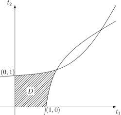
Figure 1. Domains of the integrals

For $x\in U$, we set

$$f_{i}(x)=\int_{\mathit{\Delta}_{i}}t_{1}^{-c_{1}}t_{2}^{-c_{2}}(1-t_{1}-t_{2})^{c_{1}+c_{2}-a-2}\big{(}1-\frac{x_{1}}{t_{1}}-\frac{x_{2}}{t_{2}}\big{)}^{-b}dt_{1}\wedge dt_{2},\quad(i=1,\dots,5),$$ (2.6)

where $\mathit{\Delta}_{2}$, $\mathit{\Delta}_{3}$, and $\mathit{\Delta}_{5}$ are given in Figure 2, and $\mathit{\Delta}_{4}$ is the image of $\mathit{\Delta}_{1}$ under the involution

$$\imath:(t_{1},t_{2})\mapsto(\frac{x_{1}}{t_{1}},\frac{x_{2}}{t_{2}}),$$

on

$$\mathbb{C}_{x}^{2}=\{(t_{1},t_{2})\in\mathbb{C}^{2}\mid t_{1}t_{2}(1-t_{1}-t_{2})(t_{1}t_{2}-t_{1}x_{2}-t_{2}x_{1})\neq 0\}.$$

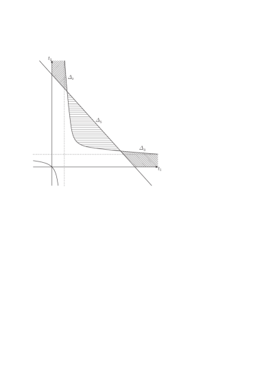
The arguments of the factors of the integrand $\displaystyle{\begin{array}[]{|c|c|c|c|c|}\hline\cr&t_{1}&t_{2}&1-t_{1}-t_{2}&1-\dfrac{x_{1}}{t_{1}}-\dfrac{x_{2}}{t_{2}}\\ \hline\cr\mathit{\Delta}_{2}&0&0&-\pi&-\pi\\ \hline\cr\mathit{\Delta}_{3}&0&0&-\pi&-\pi\\ \hline\cr\mathit{\Delta}_{5}&0&0&0&0\\ \hline\cr\end{array}}$

Figure 2. Domains of integrals

The conditions for their convergence are as follows.

$$\begin{array}[]{|c|c|}\hline\cr f_{1}&c_{1},c_{2},a-c_{1}-c_{2}\notin\mathbb{Z}\\ \hline\cr f_{2}&\mathrm{Re}(b-c_{1}+1),\mathrm{Re}(c_{1}+c_{2}-a-1),\mathrm{Re}(1-b),\mathrm{Re}(a-c_{1}+1)>0\\ \hline\cr f_{3}&\mathrm{Re}(b-c_{2}+1),\mathrm{Re}(c_{1}+c_{2}-a-1),\mathrm{Re}(1-b),\mathrm{Re}(a-c_{2}+1)>0\\ \hline\cr f_{4}&c_{1},c_{2},b-c_{1}-c_{2}\notin\mathbb{Z}\\ \hline\cr f_{5}&\mathrm{Re}(c_{1}+c_{2}-a-1),\mathrm{Re}(1-b)>0\\ \hline\cr\end{array}$$

Table 1. Convergence conditions

Lemma 2.1.

We have

$$f_{1}(x) = \frac{\mathit{\Gamma}(1-c_{1})\mathit{\Gamma}(1-c_{2})\mathit{\Gamma}(c_{1}+c_{2}-a-1)}{\mathit{\Gamma}(1-a)}F_{4}(a,b,c_{1},c_{2};x),$$

$$f_{2}(x) = \frac{\mathit{\Gamma}(a+1-c_{1})\mathit{\Gamma}(b+1-c_{1})\mathit{\Gamma}(1-b)\mathit{\Gamma}(c_{1}+c_{2}-a-1)}{\mathit{\Gamma}(2-c_{1})\mathit{\Gamma}(c_{2})}$$

$$\times e^{-\pi\sqrt{-1}(c_{1}+c_{2}-a-b)}x_{1}^{1-c_{1}}F_{4}(a+1-c_{1},b+1-c_{1},2-c_{1},c_{2};x),$$

$$f_{3}(x) = \frac{\mathit{\Gamma}(a+1-c_{2})\mathit{\Gamma}(b+1-c_{2})\mathit{\Gamma}(1-b)\mathit{\Gamma}(c_{1}+c_{2}-a-1)}{\mathit{\Gamma}(c_{1})\mathit{\Gamma}(2-c_{2})}$$

$$\times e^{-\pi\sqrt{-1}(c_{1}+c_{2}-a-b)}x_{2}^{1-c_{2}}F_{4}(a+1-c_{2},b+1-c_{2},c_{1},2-c_{2};x),$$

$$f_{4}(x) = \frac{\mathit{\Gamma}(c_{1}-1)\mathit{\Gamma}(c_{2}-1)\mathit{\Gamma}(1-b)}{\mathit{\Gamma}(c_{1}+c_{2}-b-1)}x_{1}^{1-c_{1}}x_{2}^{1-c_{2}}F_{4}(a\!+\!2\!-\!c_{1}\!-\!c_{2},b\!+\!2\!-\!c_{1}\!-\!c_{2},2\!-\!c_{1},2\!-\!c_{2};x).$$

Proof.

Note that the first equality is nothing but the integral representation (2.3). We will show the last equality. The transformation $\imath$ satisfies $\imath=\imath^{-1}$, and it implies

$$f_{4} = x_{1}^{1-c_{1}}x_{2}^{1-c_{2}}\!\!\int_{\mathit{\Delta}_{1}}t_{1}^{c_{1}-2}t_{2}^{c_{2}-2}\big{(}1-\frac{x_{1}}{t_{1}}-\frac{x_{2}}{t_{2}}\big{)}^{c_{1}+c_{2}-a-2}(1-t_{1}-t_{2})^{-b}dt_{1}\wedge dt_{2}$$

$$= x_{1}^{1-c_{1}}x_{2}^{1-c_{2}}\frac{\mathit{\Gamma}(c_{1}-1)\mathit{\Gamma}(c_{2}-1)\mathit{\Gamma}(1-b)}{\mathit{\Gamma}(c_{1}+c_{2}-b-1)}F_{4}(b\!+\!2\!-\!c_{1}\!-\!c_{2},a\!+\!2\!-\!c_{1}\!-\!c_{2},2\!-\!c_{1},2\!-\!c_{2};x).$$

To obtain the second equality, we use an orientation-reversing transformation

$$(s_{1},s_{2})\mapsto(t_{1},t_{2})=\big{(}x_{1}s_{1},\frac{1}{s_{2}}\big{)},$$

which sends the domain $D$ to $\mathit{\Delta}_{2}$. This transformation leads to

$$f_{2} = -x_{1}^{1-c_{1}}\!\!\int_{-D}s_{1}^{-c_{1}}s_{2}^{c_{2}-2}\big{(}1\!-\!x_{1}s_{1}\!-\!\frac{1}{s_{2}}\big{)}^{c_{1}\!+\!c_{2}\!-\!a\!-\!2}\big{(}1\!-\!\frac{1}{s_{1}}\!-\!s_{2}x_{2}\big{)}^{-b}ds_{1}\wedge ds_{2}$$

$$= x_{1}^{1-c_{1}}\!\!\int_{D}s_{1}^{b-c_{1}}s_{2}^{a\!-\!c_{1}}(s_{2}\!-\!x_{1}s_{1}s_{2}\!-\!1)^{c_{1}\!+\!c_{2}\!-\!a\!-\!2}(s_{1}\!-\!1-x_{2}s_{1}s_{2})^{-b}ds_{1}\wedge ds_{2}$$

$$= e^{-\pi\sqrt{-1}(c_{1}+c_{2}-a-b)}x_{1}^{1-c_{1}}\frac{\mathit{\Gamma}(b+1-c_{1})\mathit{\Gamma}(a+1-c_{1})\mathit{\Gamma}(1-b)\mathit{\Gamma}(c_{1}+c_{2}-a-1)}{\mathit{\Gamma}(2-c_{1})\mathit{\Gamma}(c_{2})}$$

$$\times F_{4}(b\!+\!1\!-\!c_{1},a\!+\!1\!-\!c_{1},2\!-\!c_{1},c_{2};x)$$

by (2.5). We can obtain the third equality in a similar way. ∎

3. Twisted homology group

Below, we will regard the parameters $a$, $b$, $c_{1}$, and $c_{2}$ as indeterminants, and we will assume that

$$a,\ a-c_{1},\ a-c_{2},\ a-c_{1}-c_{2},\ b,\ b-c_{1},\ b-c_{2},\ b-c_{1}-c_{2},\ c_{1},\ c_{2}\notin\mathbb{Z},$$ (3.1)

when we assign them to complex numbers. Set

$$\lambda_{1}=b-c_{1}+1,\quad\lambda_{2}=b-c_{2}+1,\quad\lambda_{3}=c_{1}+c_{2}-a-1,\quad\lambda_{4}=-b,$$

and let $\mathbb{C}(\mu)$ be the rational function field of $\mu_{1}=e^{2\pi\sqrt{-1}\lambda_{1}},\dots,\mu_{4}=e^{2\pi\sqrt{-1}\lambda_{4}}$ over $\mathbb{C}$.

We define a subset $\mathfrak{X}$ in $(\mathbb{P}^{1}\times\mathbb{P}^{1})\times\mathbb{P}^{2}$ by

$$\mathfrak{X}=\{(t,x)\in\mathbb{C}^{2}\times X\mid t_{1}t_{2}L(t)Q(t,x)\neq 0\},\quad L(t)=1-t_{1}-t_{2},\ Q(t,x)=t_{1}t_{2}-t_{2}x_{1}-t_{1}x_{2}.$$

There is a natural projection

$$\mathrm{pr}:\mathfrak{X}\ni(t,x)\mapsto x\in X;$$

note that $\mathbb{C}_{x}^{2}=\mathrm{pr}^{-1}(x)$ for a fixed $x\in X$. Let

$$u=u(t,x)=t_{1}^{\lambda_{1}}t_{2}^{\lambda_{2}}L(t)^{\lambda_{3}}Q(t,x)^{\lambda_{4}}=t_{1}^{b+1-c_{1}}t_{2}^{b+1-c_{2}}L(t)^{c_{1}+c_{2}-a-1}Q(t,x)^{-b}$$

be a function of $(t,x)$ in a simply connected neighborhood of $(\dot{t},\dot{x})=\frac{1}{8}(\sqrt{2},\sqrt{2},1,1)\in\mathfrak{X}$. Along any path in $\mathfrak{X}$ starting with $(\dot{t},\dot{x})$, we can make the analytic continuation of $u$. Though this continuation depends on the path, it is single valued and holomorphic around the end point of the path.

Let $\sigma$ be a $k$-chain in $\mathbb{C}_{x}^{2}$ for a fixed $x\in X$. We define a twisted $k$-chain $\sigma^{u}$ by $\sigma$ loading a branch of $u$ on it. We denote the $\mathbb{C}(\mu)$-vector space of finite sums of twisted $k$-chains by $\mathcal{C}_{k}(\mathbb{C}_{x}^{2},u)$. We define the boundary operator $\partial^{u}:\mathcal{C}_{k}(\mathbb{C}_{x}^{2},u)\to\mathcal{C}_{k-1}(\mathbb{C}_{x}^{2},u)$ by

$$\sigma^{u}\mapsto\partial(\sigma)^{u|_{\partial(\sigma)}},$$

where $\partial$ is the usual boundary operator and $u|_{\partial(\sigma)}$ is the restriction of $u$ to $\partial(\sigma)$. We have a complex

$$\mathcal{C}_{\bullet}(\mathbb{C}_{x}^{2},u):\cdots\overset{\partial^{u}}{\longrightarrow}\mathcal{C}_{k}(\mathbb{C}_{x}^{2},u)\overset{\partial^{u}}{\longrightarrow}\mathcal{C}_{k-1}(\mathbb{C}_{x}^{2},u)\overset{\partial^{u}}{\longrightarrow}\cdots,$$

and its $k$-th homology group $H_{k}(\mathcal{C}_{\bullet}(\mathbb{C}_{x}^{2},u))$. Similarly we have a complex $\mathcal{C}_{\bullet}^{lf}(\mathbb{C}_{x}^{2},u)$ of locally finite sums of twisted chains and its $k$-th homology group $H_{k}(\mathcal{C}_{\bullet}^{lf}(\mathbb{C}_{x}^{2},u))$. It is shown in [AoKi11] that

$$H_{k}(\mathcal{C}_{\bullet}(\mathbb{C}_{x}^{2},u))\simeq H_{k}(\mathcal{C}_{\bullet}^{lf}(\mathbb{C}_{x}^{2},u)),\quad\dim_{\mathbb{C}(\mu)}H_{k}(\mathcal{C}_{\bullet}(\mathbb{C}_{x}^{2},u))=\left\{\begin{array}[]{cl}4&\textrm{if }k=2,\\ 0&\textrm{otherwise,}\end{array}\right.$$

for any fixed $x\in X$. Thus we have a map

$$\mathrm{reg}:H_{2}(\mathcal{C}_{\bullet}^{lf}(\mathbb{C}_{x}^{2},u))\to H_{2}(\mathcal{C}_{\bullet}(\mathbb{C}_{x}^{2},u)),$$

which is the inverse of the natural map $H_{2}(\mathcal{C}_{\bullet}(\mathbb{C}_{x}^{2},u))\to H_{2}(\mathcal{C}_{\bullet}^{lf}(\mathbb{C}_{x}^{2},u))$.

We regard the integral (2.6) as the pairing between the form

$$\varphi_{1}=d\log\big{(}\frac{t_{1}}{L(t)}\big{)}\wedge d\log\big{(}\frac{t_{2}}{L(t)}\big{)}=\frac{dt_{1}\wedge dt_{2}}{t_{1}t_{2}L(t)}$$

and $\mathit{\Delta}_{i}$ loaded with a branch of $u$, which represents an element of $H_{2}(\mathcal{C}_{\bullet}^{lf}(\mathbb{C}_{x}^{2},u))$ $(i=1,\dots,5)$. The images of the element above under the map $\mathrm{reg}$ will be denoted by $\mathit{\Delta}_{i}^{u}\in H_{2}(\mathcal{C}_{\bullet}(\mathbb{C}_{x}^{2},u))$ for $i=1,\dots,5$.

By considering $1/u$ instead of $u$, we have $H_{2}(\mathcal{C}_{\bullet}(\mathbb{C}_{x}^{2},1/u))$ and its elements $\mathit{\Delta}_{1}^{1/u}$,…,$\mathit{\Delta}_{5}^{1/u}$. There is the intersection pairing $\mathcal{I}_{h}$ between $H_{2}(\mathcal{C}_{\bullet}(\mathbb{C}_{x}^{2},u))$ and $H_{2}(\mathcal{C}_{\bullet}(\mathbb{C}_{x}^{2},1/u))$. It is defined as follows. Let $\mathit{\Delta}^{u}$ and $\acute{\mathit{\Delta}}^{1/u}$ be elements of $H_{2}(\mathcal{C}_{\bullet}(\mathbb{C}_{x}^{2},u))$ and $H_{2}(\mathcal{C}_{\bullet}(\mathbb{C}_{x}^{2},1/u))$ given by

$$\mathit{\Delta}^{u}=\sum_{i\in I}d_{i}D_{i}^{u_{i}},\quad\acute{\mathit{\Delta}}^{1/u}=\sum_{j\in J}\acute{d}_{j}\acute{D}_{j}^{1/u_{j}},\qquad d_{i},\acute{d}_{j}\in\mathbb{C}(\mu),$$

where $D_{i}^{u_{i}}$ denotes a singular $2$-simplex $D_{i}$ loaded with a branch $u_{i}$ of $u$. Then their intersection number is

$$\mathcal{I}_{h}(\mathit{\Delta}^{u},\acute{\mathit{\Delta}}^{1/u})=\sum_{i\in I,j\in J}\sum_{p\in D_{i}\cap\acute{D}_{j}}d_{i}\acute{d}_{j}(D_{i}\cdot\acute{D}_{j})_{p}\frac{u_{i}(p)}{u_{j}(p)},$$

where $(D_{i}\cdot\acute{D}_{j})_{p}$ is the topological intersection number of $2$-chains $D_{i}$ and $\acute{D_{j}}$ at $p$. The intersection from $\mathcal{I}_{h}$ is bilinear. Since

$$\mathit{\Delta}^{1/u}=\sum_{i\in I}d_{i}^{\vee}D_{i}^{1/u_{i}},\quad\acute{\mathit{\Delta}}^{u}=\sum_{j\in J}\acute{d}_{j}^{\vee}\acute{D}_{j}^{u_{j}},$$

for the above $\mathit{\Delta}^{u}$ and $\acute{\mathit{\Delta}}^{1/u}$, we have

$$\mathcal{I}_{h}(\acute{\mathit{\Delta}}^{u},\mathit{\Delta}^{1/u})=\mathcal{I}_{h}(\mathit{\Delta}^{u},\acute{\mathit{\Delta}}^{1/u})^{\vee},$$ (3.2)

where $z(\mu_{1},\dots,\mu_{4})^{\vee}=z(1/\mu_{1},\dots,1/\mu_{4})$ for $z(\mu_{1},\dots,\mu_{4})\in\mathbb{C}(\mu)$.

Lemma 3.1.

The intersection numbers $\mathcal{I}_{h}(\mathit{\Delta}_{i}^{u},\mathit{\Delta}_{i}^{1/u})$ ($i=1,\dots,4$) are

$$\mathcal{I}_{h}(\mathit{\Delta}_{1}^{u},\mathit{\Delta}_{1}^{1/u}) = \dfrac{1-(\mu_{1}\mu_{4})(\mu_{2}\mu_{4})(\mu_{3})}{(1-\mu_{1}\mu_{4})(1-\mu_{2}\mu_{4})(1-\mu_{3})}=\dfrac{-(1-\alpha)\gamma_{1}\gamma_{2}}{(\alpha-\gamma_{1}\gamma_{2})(1-\gamma_{1})(1-\gamma_{2})},$$

$$\mathcal{I}_{h}(\mathit{\Delta}_{2}^{u},\mathit{\Delta}_{2}^{1/u}) = \dfrac{(1-\mu_{1}\mu_{4})(1-\mu_{3}(\mu_{2}\mu_{3}\mu_{4})^{-1})}{(1\!-\!\mu_{1})(1\!-\!\mu_{4})(1\!-\!\mu_{3})(1\!-\!(\mu_{2}\mu_{3}\mu_{4})^{-1})}=\dfrac{\alpha\beta\gamma_{1}(1-\gamma_{1})(1-\gamma_{2})}{(\alpha\!-\!\gamma_{1})(\alpha\!-\!\gamma_{1}\gamma_{2})(\beta\!-\!\gamma_{1})(1\!-\!\beta)},$$

$$\mathcal{I}_{h}(\mathit{\Delta}_{3}^{u},\mathit{\Delta}_{3}^{1/u}) = \dfrac{(1-\mu_{2}\mu_{4})(1-\mu_{3}(\mu_{1}\mu_{3}\mu_{4})^{-1})}{(1\!-\!\mu_{2})(1\!-\!\mu_{4})(1\!-\!\mu_{3})(1\!-\!(\mu_{1}\mu_{3}\mu_{4})^{-1})}=\dfrac{\alpha\beta\gamma_{2}(1-\gamma_{1})(1-\gamma_{2})}{(\alpha\!-\!\gamma_{2})(\alpha\!-\!\gamma_{1}\gamma_{2})(1\!-\!\beta)(\beta\!-\!\gamma_{2})},$$

$$\mathcal{I}_{h}(\mathit{\Delta}_{4}^{u},\mathit{\Delta}_{4}^{1/u}) = \dfrac{1-(\mu_{1}\mu_{4})^{-1}(\mu_{2}\mu_{4})^{-1}(\mu_{4})}{(1-(\mu_{1}\mu_{4})^{-1})(1-(\mu_{2}\mu_{4})^{-1})(1-\mu_{4})}=\dfrac{-(\beta-\gamma_{1}\gamma_{2})}{(1-\beta)(1-\gamma_{1})(1-\gamma_{2})}.$$

Proof.

To compute $\mathcal{I}_{h}(\mathit{\Delta}_{1}^{u},\mathit{\Delta}_{1}^{1/u})$, we have only to follow Example 3.1 in Section 3 of Chapter VIII of [Y97], by considering the contribution of the divisor $Q(t,x)=0$. By using the involution $\imath$, we can evaluate $\mathcal{I}_{h}(\mathit{\Delta}_{4}^{u},\mathit{\Delta}_{4}^{1/u})$. For the rest, transform $\mathit{\Delta}_{i}$ $(i=2,3)$ to the domain $D$ in the expression (2.5) as in the proof of Lemma 2.1; regard it as a quadrilateral and apply Example 3.2 in Section 3 of Chapter VIII of [Y97]. ∎

For a small simply connected neighborhood $U$ of $\dot{x}$, we have a family

$$\bigcup_{x\in U}H_{2}(\mathcal{C}_{\bullet}(\mathbb{C}_{x}^{2},u)),$$

which can be naturally identified with $\mathcal{F}_{4}(a,b,c;U)$ by (2.6). Since a path $\rho_{x}$ in $X$ connecting $\dot{x}$ and $x$ defines the isomorphism

$$(\rho_{x})_{*}:H_{2}(\mathcal{C}_{\bullet}(\mathbb{C}_{\dot{x}}^{2},u))\to H_{2}(\mathcal{C}_{\bullet}(\mathbb{C}_{x}^{2},u)),$$

we have a local system

$$\mathcal{H}_{2}(X)=\bigcup_{x\in X}H_{2}(\mathcal{C}_{\bullet}(\mathbb{C}_{x}^{2},u))$$

over $X$. Its stalk over $x$ is denoted by $H_{2}(\mathcal{C}_{\bullet}(\mathbb{C}_{x}^{2},u))$.

Similarly, we have a local system

$$\mathcal{H}_{2}^{\vee}(X)=\bigcup_{x\in X}H_{2}(\mathcal{C}_{\bullet}(\mathbb{C}_{x}^{2},1/u))$$

over $X$ with respect to $1/u$. The local triviality of these local systems $\mathcal{H}_{2}(X)$ and $\mathcal{H}_{2}^{\vee}(X)$ imply the following.

Proposition 3.1.

The intersection number is invariant under the deformation, that is,

$$\mathcal{I}_{h}((\rho_{x})_{*}(\mathit{\Delta}^{u}),(\rho_{x})_{*}(\acute{\mathit{\Delta}}^{1/u}))=\mathcal{I}_{h}(\mathit{\Delta}^{u},\acute{\mathit{\Delta}}^{1/u})$$

for any $\mathit{\Delta}^{u}\in H_{2}(\mathcal{C}_{\bullet}(\mathbb{C}_{\dot{x}}^{2},u))$, $\acute{\mathit{\Delta}}^{1/u}\in H_{2}(\mathcal{C}_{\bullet}(\mathbb{C}_{\dot{x}}^{2},1/u))$, and any path $\rho_{x}$ in $X$ connecting $\dot{x}$ and $x$.

4. Monodromy representation

A loop $\rho$ in $X$ with base point $\dot{x}$ induces a linear transformation of the stalk $H_{2}(\mathcal{C}_{\bullet}(\mathbb{C}_{\dot{x}}^{2},u))$ of $\mathcal{H}_{2}(X)$ over $\dot{x}$. By this correspondence, we have a homomorphism

$$\mathcal{M}:\pi_{1}(X,\dot{x})\to GL(H_{2}(\mathcal{C}_{\bullet}(\mathbb{C}_{\dot{x}}^{2},u))),$$

which is called the monodromy representation of the local system $\mathcal{H}_{2}(X)$. Note that we can regard it as the monodromy representation of the system $\mathcal{F}_{4}(a,b,c)$ by the identification of $\mathcal{F}_{4}(a,b,c;U)$ for a small neighborhood $U$ of $\dot{x}$ with $\bigcup_{x\in U}H_{2}(\mathcal{C}_{\bullet}(\mathbb{C}_{x}^{2},u))$. It is shown in [Kan81] that the fundamental group $\pi_{1}(X,\dot{x})$ is generated by three loops $\rho_{i}:[0,1]\to X$ ($i=1,2,3$),

$$\rho_{1} : \theta\mapsto\left(\frac{\exp(2\pi\sqrt{-1}\theta)}{8},\frac{1}{8}\right),$$

$$\rho_{2} : \theta\mapsto\left(\frac{1}{8},\frac{\exp(2\pi\sqrt{-1}\theta)}{8}\right),$$

$$\rho_{3} : \theta\mapsto\left(\frac{2-\exp(2\pi\sqrt{-1}\theta)}{8},\frac{2-\exp(2\pi\sqrt{-1}\theta)}{8}\right).$$

Note that the loop $\rho_{i}$ $(i=1,2)$ turns the divisor $x_{i}=0$ positively, and $\rho_{3}$ turns the divisor $R(x)=0$ positively. We put $\mathcal{M}_{i}=\mathcal{M}(\rho_{i})$ $(i=1,2,3)$.

Proposition 4.1.

The elements $\mathit{\Delta}_{1}^{u},\dots,\mathit{\Delta}_{4}^{u}$ span $H_{2}(\mathcal{C}_{\bullet}(\mathbb{C}_{\dot{x}}^{2},u))$. With respect to the basis $\;{}^{t}(\mathit{\Delta}_{1}^{u},\dots,\mathit{\Delta}_{4}^{u})$, $\mathcal{M}_{1}$ and $\mathcal{M}_{2}$ are represented by matrices

$$\mathrm{diag}(1,\gamma_{1}^{-1},1,\gamma_{1}^{-1})\quad\textrm{and}\quad\mathrm{diag}(1,1,\gamma_{2}^{-1},\gamma_{2}^{-1}),$$

respectively, where $\mathrm{diag}(z_{1},\dots,z_{n})$ denotes the diagonal matrix with diagonal entries $z_{1},\dots,z_{n}$.

Proof.

Recall that the solutions $f_{i}$ are defined by the integrals over $\mathit{\Delta}_{i}$ in (2.6), and that they admit local expressions as in Lemma 2.1. We have

$$\;{}^{t}\left((\rho_{1})_{*}(\mathit{\Delta}_{1}^{u}),\dots,(\rho_{1})_{*}(\mathit{\Delta}_{4}^{u})\right)=\mathrm{diag}(1,\gamma_{1}^{-1},1,\gamma_{1}^{-1})\;^{t}\left(\mathit{\Delta}_{1}^{u},\dots,\mathit{\Delta}_{4}^{u}\right),$$

$$\;{}^{t}\left((\rho_{2})_{*}(\mathit{\Delta}_{1}^{u}),\dots,(\rho_{2})_{*}(\mathit{\Delta}_{4}^{u})\right)=\mathrm{diag}(1,1,\gamma_{2}^{-1},\gamma_{2}^{-1})\;^{t}\left(\mathit{\Delta}_{1}^{u},\dots,\mathit{\Delta}_{4}^{u}\right),$$

since the local behavior of $f_{i}$ is same to that of $\mathit{\Delta}_{i}$. ∎

Lemma 4.1.

If $i\neq j$ ($1\leq i,j\leq 4$) then

$$\mathcal{I}_{h}(\mathit{\Delta}_{i}^{u},\mathit{\Delta}_{j}^{1/u})=0.$$

The intersection matrix $H=\left(\mathcal{I}_{h}(\mathit{\Delta}_{i}^{u},\mathit{\Delta}_{j}^{1/u})\right)_{1\leq i,j\leq 4}$ is a diagonal matrix with entries as given in Lemma 3.1.

Proof.

By Propositions 3.1 and 4.1, we have

$$\mathcal{I}_{h}(\mathit{\Delta}_{i}^{u},\mathit{\Delta}_{j}^{1/u})=\mathcal{I}_{h}((\rho_{1})_{*}(\mathit{\Delta}_{i}^{u}),(\rho_{1})_{*}(\mathit{\Delta}_{j}^{1/u}))=\mathcal{I}_{h}(\gamma_{1}^{-1}\mathit{\Delta}_{i}^{u},\mathit{\Delta}_{j}^{1/u})=\gamma_{1}^{-1}\mathcal{I}_{h}(\mathit{\Delta}_{i}^{u},\mathit{\Delta}_{j}^{1/u})$$

for $i=2,4$ and $j=1,3$. Since $\gamma_{1}\neq 1$, $\mathcal{I}_{h}(\mathit{\Delta}_{i}^{u},\mathit{\Delta}_{j}^{1/u})=0$ for $i=2,4$ and $j=1,3$. By (3.2), we have $\mathcal{I}_{h}(\mathit{\Delta}_{i}^{u},\mathit{\Delta}_{j}^{1/u})=0$ for $i=1,3$ and $j=2,4$. To show $\mathcal{I}_{h}(\mathit{\Delta}_{i}^{u},\mathit{\Delta}_{j}^{1/u})=0$ for $(i,j)=(1,3),(2,4),(3,1),(4,2)$, use the map $(\rho_{2})_{*}$. ∎

Remark 4.1.

The eigenspace $V_{1}^{u}$ of $\mathcal{M}_{1}$ with eigenvalue $1$ is spanned by $\mathit{\Delta}_{1}^{u}$ and $\mathit{\Delta}_{3}^{u}$. The eigenspace of $\mathcal{M}_{1}$ with eigenvalue $1/\gamma_{1}$ is characterized by

$$\{\mathit{\Delta}^{u}\in H_{2}(\mathcal{C}_{\bullet}(\mathbb{C}_{\dot{x}}^{2},u))\mid\mathcal{I}_{h}(\mathit{\Delta}^{u},\mathit{\Delta}_{1}^{1/u})=\mathcal{I}_{h}(\mathit{\Delta}^{u},\mathit{\Delta}_{3}^{1/u})=0\}.$$

The eigenspace $V_{2}^{u}$ of $\mathcal{M}_{2}$ with eigenvalue $1$ is spanned by $\mathit{\Delta}_{1}^{u}$ and $\mathit{\Delta}_{2}^{u}$. The eigenspace of $\mathcal{M}_{2}$ with eigenvalue $1/\gamma_{2}$ is characterized by

$$\{\mathit{\Delta}^{u}\in H_{2}(\mathcal{C}_{\bullet}(\mathbb{C}_{\dot{x}}^{2},u))\mid\mathcal{I}_{h}(\mathit{\Delta}^{u},\mathit{\Delta}_{1}^{1/u})=\mathcal{I}_{h}(\mathit{\Delta}^{u},\mathit{\Delta}_{2}^{1/u})=0\}.$$

Note that the linear transformation $\mathcal{M}_{i}$ $(i=1,2)$ is determined by the subspace $V_{i}^{u}$, the eigenvalue $1/\gamma_{i}$ and the intersection form $\mathcal{I}_{h}$, under the condition $c_{i}\notin\mathbb{Z}$ when we assign complex values to the parameters.

We characterize the linear transformation $\mathcal{M}_{3}$ by determining its eigenvalues and eigenspaces. The following is the key lemma of this section.

Lemma 4.2.

We have

$$\mathcal{M}_{3}(\mathit{\Delta}_{5}^{u})=-\mu_{3}\mu_{4}\mathit{\Delta}_{5}^{u}=-\dfrac{\gamma_{1}\gamma_{2}}{\alpha\beta}\mathit{\Delta}_{5}^{u},\quad\mathcal{M}_{3}(\mathit{\Delta}^{u})=\mathit{\Delta}^{u}$$

for any $\mathit{\Delta}^{u}\in(\mathit{\Delta}_{5}^{1/u})^{\perp}=\{\mathit{\Delta}^{u}\in H_{2}(\mathcal{C}_{\bullet}(\mathbb{C}_{\dot{x}}^{2},u))\mid\mathcal{I}_{h}(\mathit{\Delta}^{u},\mathit{\Delta}_{5}^{1/u})=0\}.$

Proof.

We express $\mathit{\Delta}_{5}$ in terms of the coordinates $s=(s_{1},s_{2})=(t_{1}/x_{1},t_{2}/x_{2})$. Since $L(t)$ and $Q(t,x)$ are expressed as

$$1-{s_{1}}{x_{1}}-{s_{2}}{x_{2}},\quad x_{1}x_{2}(s_{1}s_{2}-s_{1}-s_{2}),$$

in terms of these coordinates, we set

$$L(s,x)=1-{s_{1}}{x_{1}}-{s_{2}}{x_{2}},\quad Q(s)=s_{1}s_{2}-s_{1}-s_{2}.$$

The intersection points $P_{1}$ and $P_{2}$ of the curves defined by $L(s,x)=0$ and $Q(s)=0$ are

$$\left(\frac{1\!+\!x_{1}\!-\!x_{2}\!+\!\sqrt{R(x)}}{2x_{1}},\frac{1\!-\!x_{1}\!+\!x_{2}\!-\!\sqrt{R(x)}}{2x_{2}}\right),\quad\left(\frac{1\!+\!x_{1}\!-\!x_{2}\!-\!\sqrt{R(x)}}{2x_{1}},\frac{1\!-\!x_{1}\!+\!x_{2}\!+\!\sqrt{R(x)}}{2x_{2}}\right).$$

Note that $R(x)=1-4x_{1}$ for $x=(x_{1},x_{1})\in\rho_{3}$. When $x_{1}=x_{2}=1/4$, $R(x)$ vanishes and $Q(s)=0$ is tangent to $L(s,x)=0$. For $\dot{x}=(1/8,1/8)$, we regard $\mathit{\Delta}_{5}$ as

$$\bigcup_{y\in l(\dot{x}_{1})}\ell(y),$$

where $l(\dot{x}_{1})$ is the segment connecting $1/4$ and $\dot{x}_{1}=1/8$, and $\ell(y)$ is the segment connecting the intersection points of $L(s,x)=0$ and $Q(s)=0$ for $x=(y,y)$ with $y\in l(\dot{x}_{1})$; see Figure 3. For a fixed $x=(x_{1},x_{1})$ in the loop $\rho_{3}$, the segment $l(x_{1})$ is expressed as

$$\frac{1}{4}+(x_{1}-\frac{1}{4})q_{1}$$

by a parameter $q_{1}\in[0,1]$. For an element $y=1/4+(x_{1}-1/4)q_{1}\in l(x_{1})$, the segment $\ell(y)$ is expressed as

$$P_{1}(y)+(P_{2}(y)-P_{1}(y))q_{2},$$

by a parameter $q_{2}\in[0,1]$, where $P_{1}(y)$ and $P_{2}(y)$ are the intersection points $P_{1}$ and $P_{2}$ for $x=(y,y)$. Hence $\mathit{\Delta}_{5}$ is expressed by $(q_{1},q_{2})\in[0,1]\times[0,1]$ as

$$(s_{1},s_{2})=\left(\frac{2(1+(1-2q_{2})\sqrt{(1-4x_{1})q_{1}})}{1-(1-4x_{1})q_{1}},\frac{2(1-(1-2q_{2})\sqrt{(1-4x_{1})q_{1}})}{1-(1-4x_{1})q_{1}}\right)$$ (4.1)

for a fixed $x=(x_{1},x_{1})$ in the loop $\rho_{3}$.

By the continuation of $\sqrt{1-4x_{1}}$ along the loop $\rho_{3}$, its sign changes. We regard this sign change in the deformation of $\mathit{\Delta}_{5}$ along $\rho_{3}$ as a bijection of $\mathit{\Delta}_{5}$ with the reversing orientation given by

$$r:[0,1]\times[0,1]\ni(q_{1},q_{2})\mapsto(q_{1},1-q_{2})\in[0,1]\times[0,1].$$

We deform the pull-backs of $s_{1}$, $s_{2}$, $L(s,x)$, and $Q(s)$ to $[0,1]\times[0,1]$ by (4.1) along $\rho_{3}$ and apply $r$ to them. It is easy to see that those of $s_{1}$ and $s_{2}$ are invariant under the deformation and the action. Since those of $L(s,x)$ and $Q(s)$ are expressed as

$$\frac{(1-q_{1})(1-4x_{1})}{1-(1-4x_{1})q_{1}},\quad\frac{16q_{1}q_{2}(1-q_{2})(1-4x_{1})}{(1-q_{1}(1-4x_{1}))^{2}},$$

their arguments increase by $2\pi$ under the deformation, and they are invariant under $r$. Thus the pull-back of $s_{1}^{\lambda_{1}}s_{2}^{\lambda_{2}}L(s,x)^{\lambda_{3}}Q(s)^{\lambda_{4}}$ to $[0,1]\times[0,1]$ by (4.1) is multiplied by $\mu_{3}\mu_{4}$ under the deformation along $\rho_{3}$ and the action $r$. By considering the orientation of $\mathit{\Delta}_{5}$, we have

$$\mathcal{M}_{3}(\mathit{\Delta}_{5}^{u})=-\mu_{3}\mu_{4}\mathit{\Delta}_{5}^{u}.$$

It is easy to see by Figure 3 that three chambers

$$\mathit{\Delta}_{6} = \{(s_{1},s_{2})\in\mathbb{R}^{2}\mid s_{1},s_{2}<0\},$$

$$\mathit{\Delta}_{7} = \{(s_{1},s_{2})\in\mathbb{R}^{2}\mid s_{1},Q(s)>0,s_{2}<0\},$$

$$\mathit{\Delta}_{8} = \{(s_{1},s_{2})\in\mathbb{R}^{2}\mid s_{2},Q(s)>0,s_{1}<0\}$$

are invariant under the deformation along $\rho_{3}$. Thus the elements $\mathit{\Delta}_{i}^{u}$ $(i=6,7,8)$ of $H_{2}(\mathcal{C}_{\bullet}(\mathbb{C}_{\dot{x}}^{2},u))$ corresponding to $\mathit{\Delta}_{i}$ are eigenvectors of $\mathcal{M}_{3}$ with eigenvalue $1$. Since they do not intersect $\mathit{\Delta}_{5}$ topologically, they belong to $(\mathit{\Delta}_{5}^{1/u})^{\perp}$. To show that they are linearly independent, we compute the intersection numbers

$$H_{ij}=\mathcal{I}_{h}(\mathit{\Delta}_{i}^{u},\mathit{\Delta}_{j}^{1/u})\quad(6\leq i,j\leq 8):$$

$$H_{66} = 1+\frac{1}{\mu_{0}-1}+\frac{1}{\mu_{1}-1}+\frac{1}{\mu_{2}-1}$$

$$+\frac{\mu_{12}-1}{(\mu_{124}-1)(\mu_{1}-1)(\mu_{2}-1)}+\frac{\mu_{01}-1}{(\mu_{014}-1)(\mu_{0}-1)(\mu_{1}-1)}+\frac{\mu_{02}-1}{(\mu_{024}-1)(\mu_{0}-1)(\mu_{2}-1))},$$

$$H_{67} = -\frac{1}{\mu_{1}-1}\left(1+\frac{1}{\mu_{124}-1}+\frac{1}{\mu_{014}-1}\right),$$

$$H_{68} = -\frac{1}{\mu_{2}-1}\left(1+\frac{1}{\mu_{124}-1}+\frac{1}{\mu_{024}-1}\right),$$

$$H_{77} = 1+\frac{1}{\mu_{1}-1}+\frac{1}{\mu_{4}-1}+\frac{\mu_{14}-1}{(\mu_{124}-1)(\mu_{1}-1)(\mu_{4}-1)}+\frac{\mu_{14}-1}{(\mu_{014}-1)(\mu_{1}-1)(\mu_{4}-1)},$$

$$H_{78} = -\frac{\mu_{1}\mu_{4}}{(\mu_{4}-1)(\mu_{124}-1)},$$

$$H_{88} = 1+\frac{1}{\mu_{2}-1}+\frac{1}{\mu_{4}-1}+\frac{\mu_{24}-1}{(\mu_{124}-1)(\mu_{2}-1)(\mu_{4}-1)}+\frac{\mu_{24}-1}{(\mu_{024}-1)(\mu_{2}-1)(\mu_{4}-1)},$$

and $H_{ji}=H_{ij}^{\vee}$ for $6\leq i<j\leq 8$, where

$$\mu_{0}=\frac{1}{\mu_{1}\mu_{2}\mu_{3}\mu_{4}^{2}}=\alpha,\quad\mu_{ij}=\mu_{i}\mu_{j},\quad\mu_{ijk}=\mu_{i}\mu_{j}\mu_{k}.$$

Since

$$\det(H_{ij})_{6\leq i,j\leq 8}=\frac{\beta^{2}(\alpha-\gamma_{1}\gamma_{2})^{2}(\alpha\beta+\gamma_{1}\gamma_{2})}{(\alpha-1)(\alpha-\gamma_{1})(\alpha-\gamma_{2})(\beta-1)^{2}(\beta-\gamma_{1})(\beta-\gamma_{2})(\beta-\gamma_{1}\gamma_{2})},$$

if $\alpha\beta+\gamma_{1}\gamma_{2}\neq 0$ when we assign complex values to the parameters, then they span the eigenspace of $\mathcal{M}_{3}$ with eigenvalue $1$ and the space $(\mathit{\Delta}_{5}^{1/u})^{\perp}$. ∎

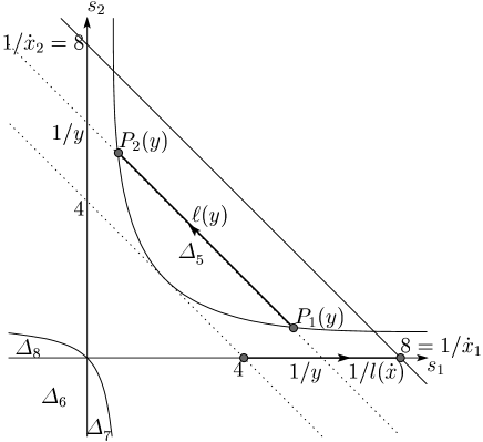
Figure 3. Cycles $\mathit{\Delta}_{5},\dots,\mathit{\Delta}_{8}$

To represent $\mathcal{M}_{3}$ by a matrix, we express $\mathit{\Delta}_{5}^{u}$ by a linear combination of $\mathit{\Delta}_{1}^{u},\dots,\mathit{\Delta}_{4}^{u}$.

Lemma 4.3.

We have

$$\mathcal{I}_{h}(\mathit{\Delta}_{5}^{u},\mathit{\Delta}_{1}^{1/u}) = \dfrac{1-(\mu_{1}\mu_{4})(\mu_{2}\mu_{4})(\mu_{3})}{(1-\mu_{1}\mu_{4})(1-\mu_{2}\mu_{4})(1-\mu_{3})}=\dfrac{-(1-\alpha)\gamma_{1}\gamma_{2}}{(\alpha-\gamma_{1}\gamma_{2})(1-\gamma_{1})(1-\gamma_{2})},$$

$$\mathcal{I}_{h}(\mathit{\Delta}_{5}^{u},\mathit{\Delta}_{2}^{1/u}) = \mathcal{I}_{h}(\mathit{\Delta}_{5}^{u},\mathit{\Delta}_{3}^{1/u})=\dfrac{\mu_{3}\mu_{4}}{(1-\mu_{3})(1-\mu_{4})}=\dfrac{-\gamma_{1}\gamma_{2}}{(\alpha-\gamma_{1}\gamma_{2})(1-\beta)},$$

$$\mathcal{I}_{h}(\mathit{\Delta}_{5}^{u},\mathit{\Delta}_{4}^{1/u}) = \dfrac{1-(\mu_{1}\mu_{4})^{-1}(\mu_{2}\mu_{4})^{-1}(\mu_{4})}{(1-(\mu_{1}\mu_{4})^{-1})(1-(\mu_{2}\mu_{4})^{-1})(1-\mu_{4})}=\dfrac{-(\beta-\gamma_{1}\gamma_{2})}{(1-\beta)(1-\gamma_{1})(1-\gamma_{2})}.$$

The twisted cycle $\mathit{\Delta}_{5}^{u}$ is expressed as

$$\mathit{\Delta}_{1}^{u}-\frac{\gamma_{2}(\alpha-\gamma_{1})(\beta-\gamma_{1})}{\alpha\beta(1-\gamma_{1})(1-\gamma_{2})}\mathit{\Delta}_{2}^{u}-\frac{\gamma_{1}(\alpha-\gamma_{2})(\beta-\gamma_{2})}{\alpha\beta(1-\gamma_{1})(1-\gamma_{2})}\mathit{\Delta}_{3}^{u}+\mathit{\Delta}_{4}^{u},$$

this leads to

$$\mathcal{I}_{h}(\mathit{\Delta}_{5}^{u},\mathit{\Delta}_{5}^{1/u})=\dfrac{1+\mu_{3}\mu_{4}}{(1-\mu_{3})(1-\mu_{4})}=\frac{-(\alpha\beta+\gamma_{1}\gamma_{2})}{(\alpha-\gamma_{1}\gamma_{2})(1-\beta)}.$$

Proof.

By the results in Section 3.4 of Chapter VIII of [Y97], we can compute the intersection numbers $\mathcal{I}_{h}(\mathit{\Delta}_{5}^{u},\mathit{\Delta}_{i}^{1/u})$ for $i=2,3$. Among the components of $\mathit{\Delta}_{1}$, only $\triangle$ intersects with $\sqrt{-1}\mathbb{R}^{2}_{x}$ at $(\sqrt{x_{1}},\sqrt{x_{2}})$. Since their topological intersection number at this point is $-1$, we have

$$(\sqrt{-1}\mathbb{R}^{2}_{x})^{1/u}=\dfrac{(1-\gamma_{1})(1-\gamma_{2})(\alpha-\gamma_{1}\gamma_{2})}{(1-\alpha)\gamma_{1}\gamma_{2}}\mathit{\Delta}_{1}^{1/u}$$

by (2.4). This implies that $\mathcal{I}_{h}(\mathit{\Delta}_{5}^{u},\mathit{\Delta}_{1}^{1/u})=\dfrac{-(1-\alpha)\gamma_{1}\gamma_{2}}{(\alpha-\gamma_{1}\gamma_{2})(1-\gamma_{1})(1-\gamma_{2})}$. We can evaluate the intersection number $\mathcal{I}_{h}(\mathit{\Delta}_{5}^{u},\mathit{\Delta}_{4}^{1/u})$ in a similar way. Lemma 4.1 together with Lemma 3.1 imply the expression of $\mathit{\Delta}_{5}^{u}$ as a linear combination of $\mathit{\Delta}_{i}^{u}$ $(i=1,\dots,4).$ ∎

Remark 4.2.

1. The eigenspace of $\mathcal{M}_{3}$ with eigenvalue $1$ is characterized by $\mathit{\Delta}_{5}^{u}$ and the intersection form $\mathcal{I}_{h}$.

2. If $\alpha\beta+\gamma_{1}\gamma_{2}=0$, then $\mathcal{I}_{h}(\mathit{\Delta}_{5}^{u},\mathit{\Delta}_{5}^{1/u})=0$. In this case, the $3$-dimensional space $(\mathit{\Delta}_{5}^{1/u})^{\perp}$ contains the cycle $\mathit{\Delta}_{5}^{u}$ and coincides with the eigenspace of $\mathcal{M}_{3}$ with eigenvalue $1$. Since $H_{2}(\mathcal{C}_{\bullet}(\mathbb{C}_{\dot{x}}^{2},u))$ is not spanned by eigenvectors of $\mathcal{M}_{3}$, its representation is not diagonalizable.

Proposition 4.2.

With respect to the basis $\;{}^{t}(\mathit{\Delta}_{1}^{u},\mathit{\Delta}_{2}^{u},\mathit{\Delta}_{3}^{u},\mathit{\Delta}_{4}^{u})$, $\mathcal{M}_{3}$ is represented by the matrix

$$\mathrm{id}_{4}-(1+\gamma_{1}\gamma_{2}\alpha^{-1}\beta^{-1})\frac{H\;^{t}e_{5}^{\vee}e_{5}}{e_{5}H\;^{t}e_{5}^{\vee}}=\mathrm{id}_{4}-\frac{(\beta-1)(\alpha-\gamma_{1}\gamma_{2})}{\alpha\beta}H\;^{t}e_{5}^{\vee}e_{5},$$

where $\mathrm{id}_{4}$ is the unit matrix of size $4$, and

$$e_{5} = \left(1,-\dfrac{\gamma_{2}(\alpha-\gamma_{1})(\beta-\gamma_{1})}{\alpha\beta(\gamma_{2}-1)(\gamma_{1}-1)},-\dfrac{\gamma_{1}(\alpha-\gamma_{2})(\beta-\gamma_{2})}{\alpha\beta(\gamma_{2}-1)(\gamma_{1}-1)},1\right),$$

$$e_{5}^{\vee} = \left(1,-\dfrac{(\alpha-\gamma_{1})(\beta-\gamma_{1})}{\gamma_{1}(\gamma_{1}-1)(\gamma_{2}-1)},-\dfrac{(\alpha-\gamma_{2})(\beta-\gamma_{2})}{\gamma_{2}(\gamma_{1}-1)(\gamma_{2}-1)},1\right),$$

corresponding to $\mathit{\Delta}_{5}^{u}$ and $\mathit{\Delta}_{5}^{1/u}$ by the expression in Lemma 4.3.

Proof.

We set $M=\mathrm{id}_{4}-(1+\gamma_{1}\gamma_{2}\alpha^{-1}\beta^{-1})H\;^{t}e_{5}^{\vee}(e_{5}H\;^{t}e_{5}^{\vee})^{-1}e_{5}$. Since

$$\mathcal{I}_{h}(\mathit{\Delta}^{u},\mathit{\Delta}_{5}^{1/u})=(d_{1},\dots,d_{4})H\;^{t}e_{5}^{\vee},$$

for $\mathit{\Delta}^{u}=(d_{1},\dots,d_{4})\;^{t}(\mathit{\Delta}_{1}^{u},\mathit{\Delta}_{2}^{u},\mathit{\Delta}_{3}^{u},\mathit{\Delta}_{4}^{u}),$ we have

$$e_{5}M = e_{5}-(1+\gamma_{1}\gamma_{2}\alpha^{-1}\beta^{-1})e_{5}H\;^{t}e_{5}^{\vee}(e_{5}H\;^{t}e_{5}^{\vee})^{-1}e_{5}=-\frac{\gamma_{1}\gamma_{2}}{\alpha\beta}e_{5},$$

$$(d_{1},\dots,d_{4})M = (d_{1},\dots,d_{4}),$$

for $(d_{1},\dots,d_{4})$ satisfying $(d_{1},\dots,d_{4})H\;^{t}e_{5}^{\vee}=0$. Thus the eigenvalues of $M$ are $-\gamma_{1}\gamma_{2}/(\alpha\beta)$ and $1$, $e_{5}$ is an eigenvector with eigenvalue $-\gamma_{1}\gamma_{2}/(\alpha\beta)$, and the eigenspace with eigenvalue $1$ is characterized by the equality $(d_{1},\dots,d_{4})H\;^{t}e_{5}^{\vee}=0$. Since $e_{5}$ corresponds to $\mathit{\Delta}_{5}$ and $(d_{1},\dots,d_{4})H\;^{t}e_{5}^{\vee}=\mathcal{I}_{h}(\mathit{\Delta}^{u},\mathit{\Delta}_{5}^{1/u})$ for $\mathit{\Delta}^{u}=d_{1}\mathit{\Delta}_{1}^{u}+\cdots+d_{4}\mathit{\Delta}_{4}^{u}$, the linear transformation represented by $M$ coincides with $\mathcal{M}_{3}$ by Lemma 4.2. Note that $\dfrac{1+\gamma_{1}\gamma_{2}\alpha^{-1}\beta^{-1}}{e_{5}H\;^{t}e_{5}^{\vee}}=\dfrac{(\beta-1)(\alpha-\gamma_{1}\gamma_{2})}{\alpha\beta}$ by Lemma 4.3. The representation matrix of $\mathcal{M}_{3}$ on the right-hand side is valid even in the case $\alpha\beta+\gamma_{1}\gamma_{2}=0$. ∎

Note that $\mathcal{M}_{1},\mathcal{M}_{2}$, and $\mathcal{M}_{3}$ are represented by the matrices in Propositions 4.1 and 4.2 with respect to the basis $\;{}^{t}(\mathit{\Delta}_{1}^{u},\mathit{\Delta}_{2}^{u},\mathit{\Delta}_{3}^{u},\mathit{\Delta}_{4}^{u})$. However, this basis degenerates when we assign an integer to $c_{i}$ $(i=1,2)$. For example, if $c_{1}=1$, then $\gamma_{1}=1$ and $\mathcal{M}_{1}$ is represented by the unit matrix; we see that this expression is not valid in this case. Hence we give expressions of $\mathcal{M}_{1},\mathcal{M}_{2}$, and $\mathcal{M}_{3}$ in terms of the intersection form $\mathcal{I}_{h}$, which are independent of the choice of a basis of $H_{2}(\mathcal{C}_{\bullet}(\mathbb{C}_{\dot{x}}^{2},u))$ and are valid even for integer values of $c_{1},c_{2}$. As we have mentioned in Remarks 4.1 and 4.2, $\mathcal{M}_{i}$ are determined by the eigenspaces $V_{1}^{u}$, $V_{2}^{u}$, the eigenvector $\mathit{\Delta}_{5}^{u}$, and the intersection form $\mathcal{I}_{h}$. We take a basis of $H_{2}(\mathcal{C}_{\bullet}(\mathbb{C}_{\dot{x}}^{2},u))$ consisting of bases of these subspaces. We set

$$\hat{\mathit{\Delta}}^{u}_{1234}=\;^{t}(\hat{\mathit{\Delta}}_{1}^{u},\hat{\mathit{\Delta}}_{2}^{u},\hat{\mathit{\Delta}}_{3}^{u},\hat{\mathit{\Delta}}_{4}^{u})=P\;^{t}(\mathit{\Delta}_{1}^{u},\mathit{\Delta}_{2}^{u},\mathit{\Delta}_{3}^{u},\mathit{\Delta}_{5}^{u}),$$

where

$$P=\begin{pmatrix}\dfrac{\alpha\beta(1-\gamma_{1})(1-\gamma_{2})}{(1-\alpha)(1-\beta)\gamma_{1}\gamma_{2}}&0&0&0\\ \dfrac{-\alpha\beta(1-\gamma_{2})}{(1-\alpha)(1-\beta)\gamma_{2}}&\dfrac{\gamma_{1}}{1-\gamma_{1}}&0&0\\ \dfrac{-\alpha\beta(1-\gamma_{1})}{(1-\alpha)(1-\beta)\gamma_{1}}&0&\dfrac{\gamma_{2}}{1-\gamma_{2}}&0\\ 0&0&0&1\\ \end{pmatrix}.$$

Lemma 4.4.

The integrals

$$\hat{f}(x)=\int_{\hat{\mathit{\Delta}}_{i}}u(t,x)\varphi_{1}\quad(i=1,2,3)$$

are well defined even in the case $c_{1},c_{2}\in\mathbb{Z}$ when we assign complex values to the parameters.

Proof.

By Lemma 2.1, we have

$$\hat{f}_{1}(x) = G_{4}\sum_{n\in\mathbb{N}^{2}}\frac{\mathit{\Gamma}(a+n_{1}+n_{2})\mathit{\Gamma}(b+n_{1}+n_{2})}{\mathit{\Gamma}(c_{1}+n_{1})\mathit{\Gamma}(c_{2}+n_{2})\mathit{\Gamma}(1+n_{1})\mathit{\Gamma}(1+n_{2})}x_{1}^{n_{1}}x_{2}^{n_{2}},$$

$$f_{2}(x) = G_{4}\sum_{n\in\mathbb{N}^{2}}\frac{\mathit{\Gamma}(a+1-c_{1}+n_{1}+n_{2})\mathit{\Gamma}(b+1-c_{1}+n_{1}+n_{2})}{\mathit{\Gamma}(2-c_{1}+n_{1})\mathit{\Gamma}(c_{2}+n_{2})\mathit{\Gamma}(1+n_{1})\mathit{\Gamma}(1+n_{2})}x_{1}^{n_{1}+1-c_{1}}x_{2}^{n_{2}},$$

$$f_{3}(x) = G_{4}\sum_{n\in\mathbb{N}^{2}}\frac{\mathit{\Gamma}(a+1-c_{2}+n_{1}+n_{2})\mathit{\Gamma}(b+1-c_{2}+n_{1}+n_{2})}{\mathit{\Gamma}(c_{1}+n_{1})\mathit{\Gamma}(2-c_{2}+n_{2})\mathit{\Gamma}(1+n_{1})\mathit{\Gamma}(1+n_{2})}x_{1}^{n_{1}}x_{2}^{n_{2}+1-c_{2}},$$

$$\hat{f}_{2}(x) = G_{4}\frac{\gamma_{1}}{1-\gamma_{1}}(f_{2}(x)-\hat{f}_{1}(x)),$$

$$\hat{f}_{3}(x) = G_{4}\frac{\gamma_{2}}{1-\gamma_{2}}(f_{3}(x)-\hat{f}_{1}(x)),$$

where $G_{4}=\mathit{\Gamma}(1-b)\mathit{\Gamma}(c_{1}+c_{2}-a-1)e^{\pi\sqrt{-1}(a+b-c_{1}-c_{2})}$. It is clear that $\hat{f}_{1}(x)$ is well defined for $c_{1},c_{2}\in\mathbb{Z}$. We claim that

$$\lim_{c_{1}\to m}\frac{f_{2}(x)-\hat{f}_{1}(x)}{c_{1}-m}$$

converges to a nonzero function for any $m\in\mathbb{Z}$. Let $m$ be a fixed integer, and put $c_{1}=m-\varepsilon$. Then $f_{2}(x)/G_{4}$ is

$$\sum_{\begin{subarray}{c}n^{\prime}_{1}\geq 1-m\\ n_{2}\geq 0\end{subarray}}\frac{\mathit{\Gamma}(a+n^{\prime}_{1}+n_{2}+\varepsilon)\mathit{\Gamma}(b+n^{\prime}_{1}+n_{2}+\varepsilon)}{\mathit{\Gamma}(1+n^{\prime}_{1}+\varepsilon)\mathit{\Gamma}(c_{2}+n_{2})\mathit{\Gamma}(n^{\prime}_{1}+m)\mathit{\Gamma}(1+n_{2})}x_{1}^{n^{\prime}_{1}+\varepsilon}x_{2}^{n_{2}},$$

where $n^{\prime}_{1}=n_{1}+1-m$. If $m\geq 2$, then we have

$$\lim_{\varepsilon\to 0}\frac{1}{\mathit{\Gamma}(1+n^{\prime}_{1}+\varepsilon)}=0$$

for $1-m\leq n_{1}^{\prime}<0$. If $m\leq 0$, then the terms $1/\mathit{\Gamma}(c_{1}+n_{1})$ ($0\leq n_{1}\leq-m$) in the series expressing $\hat{f}_{1}(x)$ converge to $0$ as $c_{1}\to m$. Thus $f_{2}(x)$ converges to $\hat{f}_{1}(x)$ with $c_{1}=m$ as $\varepsilon\to 0$. Since the poles of the $\mathit{\Gamma}$-function are simple, we have this claim. Similarly we can show that $\hat{f}_{3}(x)$ is well defined for $c_{1},c_{2}\in\mathbb{Z}$. ∎

The intersection matrix $\hat{H}=\left(\mathcal{I}_{h}(\hat{\mathit{\Delta}}_{i}^{u},\hat{\mathit{\Delta}}_{j}^{1/u})\right)_{1\leq i,j\leq 4}$ is given by

$$\begin{pmatrix}\frac{-\alpha\beta(1-\gamma_{1})(1-\gamma_{2})}{(1-\alpha)(\alpha-\gamma_{1}\gamma_{2})(1-\beta)^{2}}&\frac{-\alpha\beta(1-\gamma_{2})}{(1-\alpha)(\alpha-\gamma_{1}\gamma_{2})(1-\beta)^{2}}&\frac{-\alpha\beta(1-\gamma_{1})}{(1-\alpha)(\alpha-\gamma_{1}\gamma_{2})(1-\beta)^{2}}&\frac{-\alpha\beta}{(\alpha-\gamma_{1}\gamma_{2})(1-\beta)}\\[5.69054pt] \frac{\alpha\beta\gamma_{1}(1-\gamma_{2})}{(1-\alpha)(\alpha-\gamma_{1}\gamma_{2})(1-\beta)^{2}}&\frac{\alpha\beta(\alpha\beta-\gamma_{1})\gamma_{1}(1-\gamma_{2})}{(1-\alpha)(\alpha-\gamma_{1})(\alpha-\gamma_{1}\gamma_{2})(1-\beta)^{2}(\beta-\gamma_{1})}&\frac{\alpha\beta\gamma_{1}}{(1-\alpha)(\alpha-\gamma_{1}\gamma_{2})(1-\beta)^{2}}&0\\[5.69054pt] \frac{\alpha\beta(1-\gamma_{1})\gamma_{2}}{(1-\alpha)(\alpha-\gamma_{1}\gamma_{2})(1-\beta)^{2}}&\frac{\alpha\beta\gamma_{2}}{(1-\alpha)(\alpha-\gamma_{1}\gamma_{2})(\beta-1)^{2}}&\frac{\alpha\beta(\alpha\beta-\gamma_{2})(1-\gamma_{1})\gamma_{2}}{(1-\alpha)(\alpha-\gamma_{2})(\alpha-\gamma_{1}\gamma_{2})(\beta-1)^{2}(\beta-\gamma_{2})}&0\\[5.69054pt] \frac{-\gamma_{1}\gamma_{2}}{(\alpha-\gamma_{1}\gamma_{2})(1-\beta)}&0&0&\frac{-(\alpha\beta+\gamma_{1}\gamma_{2})}{(\alpha-\gamma_{1}\gamma_{2})(1-\beta)}\end{pmatrix},$$

and its determinant is

$$\frac{\alpha^{3}\beta^{3}(\beta-\gamma_{1}\gamma_{2})\gamma_{1}^{2}\gamma_{2}^{2}}{(1-\alpha)(\alpha-\gamma_{1})(\alpha-\gamma_{2})(\alpha-\gamma_{1}\gamma_{2})^{3}(1-\beta)^{5}(\beta-\gamma_{1})(\beta-\gamma_{2})}.$$

Let $\hat{H}_{12}$ (resp. $\hat{H}_{13}$) be the submatrix of $\hat{H}$ made by entries $(1,1)$, $(1,2)$, $(2,1)$, and $(2,2)$ (resp. $(1,1)$, $(1,3)$, $(3,1)$, and $(3,3)$).

Theorem 4.1.

The linear transformations $\mathcal{M}_{i}=\mathcal{M}(\rho_{i})$ $(i=1,2,3)$ of $H_{2}(\mathcal{C}_{\bullet}(\mathbb{C}_{\dot{x}}^{2},u))$ are expressed as

$$\mathcal{M}_{1}(\mathit{\Delta}^{u}) = \dfrac{1}{\gamma_{1}}\mathit{\Delta}^{u}+(1-\dfrac{1}{\gamma_{1}})\left(\mathcal{I}_{h}(\mathit{\Delta}^{u},\hat{\mathit{\Delta}}_{1}^{1/u}),\mathcal{I}_{h}(\mathit{\Delta}^{u},\hat{\mathit{\Delta}}_{3}^{1/u})\right)(\hat{H}_{13})^{-1}\begin{pmatrix}\hat{\mathit{\Delta}}_{1}^{u}\\ \hat{\mathit{\Delta}}_{3}^{u}\end{pmatrix},$$

$$\mathcal{M}_{2}(\mathit{\Delta}^{u}) = \dfrac{1}{\gamma_{2}}\mathit{\Delta}^{u}+(1-\dfrac{1}{\gamma_{2}})\left(\mathcal{I}_{h}(\mathit{\Delta}^{u},\hat{\mathit{\Delta}}_{1}^{1/u}),\mathcal{I}_{h}(\mathit{\Delta}^{u},\hat{\mathit{\Delta}}_{2}^{1/u})\right)(\hat{H}_{12})^{-1}\begin{pmatrix}\hat{\mathit{\Delta}}_{1}^{u}\\ \hat{\mathit{\Delta}}_{2}^{u}\end{pmatrix},$$

$$\mathcal{M}_{3}(\mathit{\Delta}^{u}) = \mathit{\Delta}^{u}-(1+\dfrac{\gamma_{1}\gamma_{2}}{\alpha\beta})\dfrac{\mathcal{I}_{h}(\mathit{\Delta}^{u},\mathit{\Delta}_{5}^{1/u})}{\mathcal{I}_{h}(\mathit{\Delta}_{5}^{u},\mathit{\Delta}_{5}^{1/u})}\mathit{\Delta}_{5}^{u}=\mathit{\Delta}^{u}-\frac{(\beta-1)(\alpha-\gamma_{1}\gamma_{2})}{\alpha\beta}\mathcal{I}_{h}(\mathit{\Delta}^{u},\mathit{\Delta}_{5}^{1/u})\mathit{\Delta}_{5}^{u}.$$

Proof.

By Proposition 4.1 and Lemma 4.1, the eigenspace of $\mathcal{M}_{1}$ with eigenvalue $1$ is spanned by $\mathit{\Delta}_{1}^{u}$ and $\mathit{\Delta}_{3}^{u}$, and that with $\gamma_{1}^{-1}$ is its orthogonal complement

$$\{\mathit{\Delta}^{u}\in H_{2}(\mathcal{C}_{\bullet}(\mathbb{C}_{\dot{x}}^{2},u))\mid\mathcal{I}_{h}(\mathit{\Delta}^{u},\mathit{\Delta}_{1}^{1/u})=\mathcal{I}_{h}(\mathit{\Delta}^{u},\mathit{\Delta}_{3}^{1/u})=0\}.$$

The elements $\hat{\mathit{\Delta}}_{1}^{u}$ and $\hat{\mathit{\Delta}}_{3}^{u}$ belong to the eigenspace of $\mathcal{M}_{1}$ with eigenvalue $1$, and they are linearly independent. Set

$$\mathcal{M}_{1}^{\prime}(\mathit{\Delta}^{u})=\dfrac{1}{\gamma_{1}}\mathit{\Delta}^{u}+(1-\dfrac{1}{\gamma_{1}})\left(\mathcal{I}_{h}(\mathit{\Delta}^{u},\hat{\mathit{\Delta}}_{1}^{1/u}),\mathcal{I}_{h}(\mathit{\Delta}^{u},\hat{\mathit{\Delta}}_{3}^{1/u})\right)(\hat{H}_{13})^{-1}\begin{pmatrix}\hat{\mathit{\Delta}}_{1}^{u}\\ \hat{\mathit{\Delta}}_{3}^{u}\end{pmatrix}.$$

We can easily check that

$$\mathcal{M}_{1}^{\prime}(\mathit{\Delta}^{u})=\left\{\begin{array}[]{ccl}\hat{\mathit{\Delta}}_{i}^{u}&\textrm{if}&\mathit{\Delta}^{u}=\hat{\mathit{\Delta}}_{i}^{u}\ (i=1,3),\\ \dfrac{1}{\gamma_{1}}\mathit{\Delta}^{u}&\textrm{if}&\mathcal{I}_{h}(\mathit{\Delta}^{u},\hat{\mathit{\Delta}}_{1}^{1/u})=\mathcal{I}_{h}(\mathit{\Delta}^{u},\hat{\mathit{\Delta}}_{3}^{1/u})=0,\end{array}\right.$$

by the property

$$\left(\mathcal{I}_{h}(\mathit{\Delta}^{u},\hat{\mathit{\Delta}}_{1}^{1/u}),\mathcal{I}_{h}(\mathit{\Delta}^{u},\hat{\mathit{\Delta}}_{3}^{1/u})\right)(\hat{H}_{13})^{-1}=\left\{\begin{array}[]{ccl}(1,0)&\textrm{if}&\mathit{\Delta}^{u}=\hat{\mathit{\Delta}}_{1}^{u},\\ (0,1)&\textrm{if}&\mathit{\Delta}^{u}=\hat{\mathit{\Delta}}_{3}^{u},\\ (0,0)&\textrm{if}&\mathcal{I}_{h}(\mathit{\Delta}^{u},\hat{\mathit{\Delta}}_{1}^{1/u})=\mathcal{I}_{h}(\mathit{\Delta}^{u},\hat{\mathit{\Delta}}_{3}^{1/u})=0.\end{array}\right.$$

Since the eigenvalues and eigenspaces of $\mathcal{M}_{1}$ coincide with those of $\mathcal{M}_{1}^{\prime}$, we have $\mathcal{M}_{1}=\mathcal{M}_{1}^{\prime}$. We obtain the expression of $\mathcal{M}_{2}$ in a similar way. Set

$$\mathcal{M}^{\prime}_{3}(\mathit{\Delta}^{u})=\mathit{\Delta}^{u}-(1+\dfrac{\gamma_{1}\gamma_{2}}{\alpha\beta})\frac{\mathcal{I}_{h}(\mathit{\Delta}^{u},\mathit{\Delta}_{5}^{1/u})}{\mathcal{I}_{h}(\mathit{\Delta}_{5}^{u},\mathit{\Delta}_{5}^{1/u})}\mathit{\Delta}_{5}^{u}.$$

By the property

$$\frac{\mathcal{I}_{h}(\mathit{\Delta}^{u},\mathit{\Delta}_{5}^{1/u})}{\mathcal{I}_{h}(\mathit{\Delta}_{5}^{u},\mathit{\Delta}_{5}^{1/u})}=\left\{\begin{array}[]{ccl}1&\textrm{if}&\mathit{\Delta}^{u}=\mathit{\Delta}_{5}^{u},\\ 0&\textrm{if}&\mathit{\Delta}^{u}\in(\mathit{\Delta}_{5}^{1/u})^{\perp},\end{array}\right.$$

we see that

$$\mathcal{M}_{3}^{\prime}(\mathit{\Delta}^{u})=\left\{\begin{array}[]{ccl}-\dfrac{\gamma_{1}\gamma_{2}}{\alpha\beta}\mathit{\Delta}_{5}^{u}&\textrm{if}&\mathit{\Delta}^{u}=\mathit{\Delta}_{5}^{u},\\ \mathit{\Delta}^{u}&\textrm{if}&\mathit{\Delta}^{u}\in(\mathit{\Delta}_{5}^{1/u})^{\perp},\end{array}\right.$$

which shows $\mathcal{M}_{3}=\mathcal{M}_{3}^{\prime}$ by Lemma 4.2. The second expression of $\mathcal{M}_{3}$ is obtained by the equality $\mathcal{I}_{h}(\mathit{\Delta}_{5}^{u},\mathit{\Delta}_{5}^{1/u})=\dfrac{-(\alpha\beta+\gamma_{1}\gamma_{2})}{(\alpha-\gamma_{1}\gamma_{2})(1-\beta)}$ in Lemma 4.3. ∎

Remark 4.3.

1. We note that when we assign integers to $c_{1}$ and $c_{2}$, although $\mathit{\Delta}_{1}^{u}$, $\mathit{\Delta}_{2}^{u}$, and $\mathit{\Delta}_{3}^{u}$ are linearly dependent, $\hat{\mathit{\Delta}}_{1}^{u}$, $\hat{\mathit{\Delta}}_{2}^{u}$, and $\hat{\mathit{\Delta}}_{3}^{u}$ remain linearly independent.

2. Since we have

   $$(\hat{H}_{12})^{-1} = \frac{(\alpha-\gamma_{1}\gamma_{2})(1-\beta)}{\alpha\beta\gamma_{1}^{2}(1-\gamma_{2})}\begin{pmatrix}(\alpha\beta-\gamma_{1})\gamma_{1}&(\alpha-\gamma_{1})(\beta-\gamma_{1})\\ -(\alpha-\gamma_{1})(\beta-\gamma_{1})\gamma_{1}&-(\alpha-\gamma_{1})(\beta-\gamma_{1})(1-\gamma_{1})\end{pmatrix},$$

   $$(\hat{H}_{13})^{-1} = \frac{(\alpha-\gamma_{1}\gamma_{2})(1-\beta)}{\alpha\beta(1-\gamma_{1})\gamma_{2}^{2}}\begin{pmatrix}(\alpha\beta-\gamma_{2})\gamma_{2}&(\alpha-\gamma_{2})(\beta-\gamma_{2})\\ -(\alpha-\gamma_{2})(\beta-\gamma_{2})\gamma_{2}&-(\alpha-\gamma_{2})(\beta-\gamma_{2})(1-\gamma_{2})\end{pmatrix},$$

   the factors $1-\gamma_{1}$ and $1-\gamma_{2}$ are canceled in the expression of $\mathcal{M}_{1}$ and $\mathcal{M}_{2}$. Theorem 4.1 is valid even in the case $c_{1},c_{2},a+b-c_{1}-c_{2}-\dfrac{1}{2}\in\mathbb{Z}$ when we assign complex values to the parameters.

Corollary 4.1.

The linear transformations $\mathcal{M}_{i}$ $(i=1,2,3)$ are represented by matrices $M_{i}$ with respect to the basis $\hat{\mathit{\Delta}}^{u}_{1234}=\;^{t}(\hat{\mathit{\Delta}}_{1}^{u},\dots,\hat{\mathit{\Delta}}_{4}^{u})$ as $\mathcal{M}_{i}(\hat{\mathit{\Delta}}^{u}_{1234})=M_{i}\hat{\mathit{\Delta}}^{u}_{1234},$ where

$$M_{1} = \frac{1}{\gamma_{1}}\mathrm{id}_{4}+(1-\frac{1}{\gamma_{1}})\hat{H}(\;^{t}e_{1},\;^{t}e_{3})(\hat{H}_{13})^{-1}\begin{pmatrix}e_{1}\\ e_{3}\end{pmatrix}=\begin{pmatrix}1&0&0&0\\ 1&\frac{1}{\gamma_{1}}&0&0\\ 0&0&1&0\\ \frac{\alpha\beta-\gamma_{2}}{\alpha\beta}&0&\frac{(\alpha-\gamma_{2})(\beta-\gamma_{2})}{\alpha\beta\gamma_{2}}&\frac{1}{\gamma_{1}}\end{pmatrix},$$

$$M_{2} = \frac{1}{\gamma_{2}}\mathrm{id}_{4}+(1-\frac{1}{\gamma_{2}})\hat{H}(\;^{t}e_{1},\;^{t}e_{2})(\hat{H}_{12})^{-1}\begin{pmatrix}e_{1}\\ e_{2}\end{pmatrix}=\begin{pmatrix}1&0&0&0\\ 0&1&0&0\\ 1&0&\frac{1}{\gamma_{2}}&0\\ \frac{\alpha\beta-\gamma_{1}}{\alpha\beta}&\frac{(\alpha-\gamma_{1})(\beta-\gamma_{1})}{\alpha\beta\gamma_{1}}&0&\frac{1}{\gamma_{2}}\end{pmatrix},$$

$$M_{3} = \mathrm{id}_{4}-(1+\frac{\gamma_{1}\gamma_{2}}{\alpha\beta})\frac{\hat{H}\;^{t}e_{4}e_{4}}{e_{4}\hat{H}\;^{t}e_{4}}=\begin{pmatrix}1&0&0&-1\\ 0&1&0&0\\ 0&0&1&0\\ 0&0&0&\frac{-\gamma_{1}\gamma_{2}}{\alpha\beta}\end{pmatrix},$$

and $e_{i}$ is the $i$-th unit row vector of $\mathbb{Z}^{4}$.

Proof.

The matrix $M_{3}$ is obtained in the same way as in the proof of Proposition 4.2. By the expression of $\mathcal{M}_{1}$ in Theorem 4.1, we give its representation matrix with respect to the basis $\hat{\mathit{\Delta}}^{u}_{1234}$. Set ${\mathit{\Delta}}^{u}=(d_{1},\dots,d_{4})\hat{\mathit{\Delta}}^{u}_{1234}$. Since

$$\mathcal{I}_{h}(\mathit{\Delta}^{u},\hat{\mathit{\Delta}}_{i}^{1/u})=(d_{1},\dots,d_{4})\hat{H}\;^{t}e_{i}\quad(i=1,\dots,4)$$

we have

$$\left(\mathcal{I}_{h}(\mathit{\Delta}^{u},\hat{\mathit{\Delta}}_{1}^{1/u}),\mathcal{I}_{h}(\mathit{\Delta}^{u},\hat{\mathit{\Delta}}_{3}^{1/u})\right)=(d_{1},\dots,d_{4})\hat{H}(\;^{t}e_{1},\;^{t}e_{3}).$$

Note that

$$\begin{pmatrix}\hat{\mathit{\Delta}}_{1}^{u}\\ \hat{\mathit{\Delta}}_{3}^{u}\end{pmatrix}=\begin{pmatrix}e_{1}\\ e_{3}\end{pmatrix}\hat{\mathit{\Delta}}^{u}_{1234}.$$

Thus we have

$$\left(\mathcal{I}_{h}(\mathit{\Delta}^{u},\hat{\mathit{\Delta}}_{1}^{1/u}),\mathcal{I}_{h}(\mathit{\Delta}^{u},\hat{\mathit{\Delta}}_{3}^{1/u})\right)(\hat{H}_{13})^{-1}\begin{pmatrix}\hat{\mathit{\Delta}}_{1}^{u}\\ \hat{\mathit{\Delta}}_{3}^{u}\end{pmatrix}=(d_{1},\dots,d_{4})\hat{H}(\;^{t}e_{1},\;^{t}e_{3})(\hat{H}_{13})^{-1}\begin{pmatrix}e_{1}\\ e_{3}\end{pmatrix}\hat{\mathit{\Delta}}^{u}_{1234},$$

which implies that $M_{1}$ is the representation matrix of $\mathcal{M}_{1}$. We obtain the matrix $M_{2}$ in a similar way. ∎

Remark 4.4.

With respect to the basis $P^{\prime}\;{}^{t}(\mathit{\Delta}_{1}^{u},\mathit{\Delta}_{2}^{u},\mathit{\Delta}_{3}^{u},\mathit{\Delta}_{4}^{u})$ of $H_{2}(\mathcal{C}_{\bullet}(\mathbb{C}_{\dot{x}}^{2},u))$ for

$$P^{\prime}=\left(\begin{array}[]{cccc}\dfrac{\alpha\beta(1\!-\!\gamma_{1})(1\!-\!\gamma_{2})}{(1\!-\!\alpha)(1\!-\!\beta)\gamma_{1}\gamma_{2}}&0&0&0\\ \dfrac{-\alpha\beta(1\!-\!\gamma_{2})}{(1\!-\!\alpha)(1\!-\!\beta)\gamma_{2}}&\dfrac{\gamma_{1}}{1\!-\!\gamma_{1}}&0&0\\ \dfrac{-\alpha\beta(1\!-\!\gamma_{1})}{(1\!-\!\alpha)(1\!-\!\beta)\gamma_{1}}&0&\dfrac{\gamma_{2}}{1\!-\!\gamma_{2}}&0\\ \dfrac{\alpha\beta}{(1\!-\!\alpha)(1\!-\!\beta)}&\dfrac{-\gamma_{1}\gamma_{2}}{(1\!-\!\gamma_{1})(1\!-\!\gamma_{2})}&\dfrac{-\gamma_{1}\gamma_{2}}{(1\!-\!\gamma_{1})(1\!-\!\gamma_{2})}&\dfrac{\alpha\beta\gamma_{1}\gamma_{2}}{(\alpha\!-\!\gamma_{1}\gamma_{2})(\beta\!-\!\gamma_{1}\gamma_{2})}\end{array}\right),$$

$\mathcal{M}_{1}$, $\mathcal{M}_{2}$, and $\mathcal{M}_{3}$ are represented by matrices

$$\begin{pmatrix}1&0&0&0\\ 1&\gamma_{1}^{-1}&0&0\\ 0&0&1&0\\ 0&0&1&\gamma_{1}^{-1}\end{pmatrix},\quad\begin{pmatrix}1&0&0&0\\ 0&1&0&0\\ 1&0&\gamma_{2}^{-1}&0\\ 0&1&0&\gamma_{2}^{-1}\end{pmatrix},$$

$$\begin{pmatrix}-\frac{\gamma_{1}\gamma_{2}}{\alpha\beta}&\frac{\gamma_{1}\gamma_{2}}{\alpha\beta}-\frac{1}{\gamma_{1}}&\frac{\gamma_{1}\gamma_{2}}{\alpha\beta}-\frac{1}{\gamma_{2}}&-\frac{(\alpha-\gamma_{1}\gamma_{2})(\beta-\gamma_{1}\gamma_{2})}{\alpha\beta\gamma_{1}\gamma_{2}}\\ 0&1&0&0\\ 0&0&1&0\\ 0&0&0&1\end{pmatrix},$$

respectively. These representations of $\mathcal{M}_{i}$ are also valid even in the case $c_{1},c_{2},a+b-c_{1}-c_{2}-\dfrac{1}{2}\in\mathbb{Z}$ when we assign complex values to the parameters.

5. Twisted cohomology group

Recall that

$$\lambda_{1} = b+1-c_{1},\quad\lambda_{2}=b+1-c_{2},\quad\lambda_{3}=-a+c_{1}+c_{2}-1,\quad\lambda_{4}=-b,$$

$$\mathfrak{X} = \big{\{}(t,x)\in\mathbb{C}^{2}\times X\big{|}t_{1}t_{2}L(t)Q(t,x)\neq 0\big{\}}\subset(\mathbb{P}^{1}\times\mathbb{P}^{1})\times\mathbb{P}^{2},$$

$$\mathbb{C}_{x}^{2} = \mathrm{pr}^{-1}(x),\quad\mathrm{pr}:\mathfrak{X}\ni(t,x)\mapsto x\in X.$$

In this section, we regard vector spaces as defined over the rational function field $\mathbb{C}(\lambda)=\mathbb{C}(\lambda_{1},\dots,\lambda_{4})=\mathbb{C}(a,b,c_{1},c_{2})$. We denote the vector space of rational functions on $\mathbb{P}^{2}$ with poles only along $S$ by $\mathcal{O}_{X}(*S)$. Note that $\mathcal{O}_{X}(*S)$ admits the structure of an algebra over $\mathbb{C}(\lambda)$. We set

$$\mathfrak{S}=(\mathbb{P}^{1}\times\mathbb{P}^{1})\times\mathbb{P}^{2}-\mathfrak{X}.$$

Let $\mathit{\Omega}^{k}_{\mathfrak{X}}(*\mathfrak{S})$ be the vector space of rational $k$-forms on $\mathfrak{X}$ with poles only along $\mathfrak{S}$ and $\mathit{\Omega}^{p,q}_{\mathfrak{X}}(*\mathfrak{S})$ be the subspace of $\mathit{\Omega}^{p+q}_{\mathfrak{X}}(*\mathfrak{S})$ consisting of elements that are $p$-forms with respect to the variables $t_{1},t_{2}$. We set

$$\omega=d_{t}\log(u(t,x))=\lambda_{1}\frac{dt_{1}}{t_{1}}+\lambda_{2}\frac{dt_{2}}{t_{2}}+\lambda_{3}\frac{d_{t}L(t)}{L(t)}+\lambda_{4}\frac{d_{t}Q(t,x)}{Q(t,x)}\in\mathit{\Omega}^{1,0}_{\mathfrak{X}}(*\mathfrak{S}),$$

where $d_{t}$ is the exterior derivative with respect to the variables $t_{1},t_{2}$. Note that

$$d_{t}L(t)=-dt_{1}-dt_{2},\quad d_{t}Q(t,x)=(t_{2}-x_{2})dt_{1}+(t_{1}-x_{1})dt_{2}.$$

By a twisted exterior derivative ${\rm NewA}=d_{t}+\omega\wedge$ on $\mathfrak{X}$, we define quotient spaces

$$\mathcal{H}^{k}({\rm NewA})=\ker\left({\rm NewA}:\mathit{\Omega}_{\mathfrak{X}}^{k,0}(*\mathfrak{S})\to\mathit{\Omega}_{\mathfrak{X}}^{k+1,0}(*\mathfrak{S})\right)\big{/}{\rm NewA}\left(\mathit{\Omega}_{\mathfrak{X}}^{k-1,0}(*\mathfrak{S})\right)\quad(k=0,1,2),$$

where we regard $\mathit{\Omega}_{\mathfrak{X}}^{-1,0}(*\mathfrak{S})$ as the zero vector space. Each of them admits the structure of a vector bundle over $X$.

We consider the structure of the fiber of $\mathcal{H}^{k}({\rm NewA})$ at $x$. Let $\mathit{\Omega}_{\mathbb{C}_{x}^{2}}^{p}(*x)$ be the vector space of rational $p$-forms on $\mathbb{C}_{x}^{2}$ with poles only along the pole divisor of the pull-back $\omega_{x}=\imath_{x}^{*}(\omega)$ of $\omega$ by the map $\imath_{x}:\mathbb{C}_{x}^{2}\to\mathfrak{X}$. There is a natural map from each fiber of $\mathcal{H}^{k}({\rm NewA})$ at $x$ to the rational twisted cohomology group

$$H^{k}(\mathit{\Omega}_{\mathbb{C}_{x}^{2}}^{\bullet}(*x),{\rm NewA}_{x})=\ker\left({\rm NewA}_{x}:\mathit{\Omega}_{\mathbb{C}_{x}^{2}}^{k}(*x)\to\mathit{\Omega}_{\mathbb{C}_{x}^{2}}^{k+1}(*x)\right)/{\rm NewA}_{x}\left(\mathit{\Omega}_{\mathbb{C}_{x}^{2}}^{k-1}(*x)\right)$$

on $\mathbb{C}_{x}^{2}$ with respect to the twisted exterior derivative ${\rm NewA}_{x}=d_{t}+\omega_{x}\wedge$.

Facts 5.1 ([AoKi11],[Cho97]).

• We have

  $$\dim H^{k}(\mathit{\Omega}_{\mathbb{C}_{x}^{2}}^{\bullet}(*x),{\rm NewA}_{x})=\left\{\begin{array}[]{ccl}4&\textrm{if}&k=2,\\ 0&\textrm{if}&k=0,1.\end{array}\right.$$

• There is a canonical isomorphism

  $$\jmath_{x}:H^{2}(\mathit{\Omega}_{\mathbb{C}_{x}^{2}}^{\bullet}(*x),{\rm NewA}_{x})\to H^{2}(\mathcal{E}_{c}^{\bullet}(x),{\rm NewA}_{x})=\ker({\rm NewA}_{x}:\mathcal{E}_{c}^{2}(x)\to\mathcal{E}_{c}^{3}(x))/{\rm NewA}_{x}(\mathcal{E}_{c}^{1}(x)),$$

  where $\mathcal{E}_{c}^{k}(x)$ is the vector space of smooth $k$-forms with compact support in $\mathbb{C}_{x}^{2}$.

We have a twisted exterior derivative ${\rm NewA}^{\vee}=d_{t}-\omega\wedge$ for $-\omega$ and

$$\mathcal{H}^{2}({\rm NewA}^{\vee})=\mathit{\Omega}_{\mathfrak{X}}^{2,0}(*\mathfrak{S})\big{/}{\rm NewA}^{\vee}(\mathit{\Omega}_{\mathfrak{X}}^{1,0}(*\mathfrak{S})),\quad H^{2}(\mathit{\Omega}_{\mathbb{C}_{x}^{2}}^{\bullet}(*x),{\rm NewA}_{x}^{\vee})=\mathit{\Omega}_{\mathbb{C}_{x}^{2}}^{2}(*x)/{\rm NewA}_{x}^{\vee}(\mathit{\Omega}_{\mathbb{C}_{x}^{2}}^{1}(*x)).$$

The $\mathcal{O}_{X}(*S)$-module $\mathcal{H}^{2}({\rm NewA}^{\vee})$ can be regarded as a vector bundle over $X$.

For any fixed $x\in X$, we define the intersection form between $H^{2}(\mathit{\Omega}_{\mathbb{C}_{x}^{2}}^{\bullet}(*x),{\rm NewA})$ and $H^{2}(\mathit{\Omega}_{\mathbb{C}_{x}^{2}}^{\bullet}(*x),{\rm NewA}^{\vee})$ by

$$\mathcal{I}_{c}(\varphi_{x},\varphi_{x}^{\prime})=\int_{\mathbb{C}_{x}^{2}}\jmath_{x}(\varphi_{x})\wedge\varphi_{x}^{\prime}\in\mathbb{C}(\alpha),$$

where $\varphi_{x},\varphi_{x}^{\prime}\in\mathit{\Omega}_{\mathbb{C}_{x}^{2}}^{2}(*x)$, $\jmath_{x}$ is given in Fact 5.1. This integral converges since $\jmath_{x}(\varphi_{x})$ is a smooth $2$-from on $\mathbb{C}_{x}^{2}$ with compact support. It is bilinear over $\mathbb{C}(\alpha)$.

We take four elements

$$\begin{array}[]{ll}\varphi_{1}=d_{t}\log\big{(}\dfrac{t_{1}}{L(t)}\big{)}\wedge d_{t}\log\big{(}\dfrac{t_{2}}{L(t)}\big{)}=\dfrac{dt_{1}\wedge dt_{2}}{t_{1}t_{2}L(t)},&\varphi_{2}=d_{t}\log(t_{2})\wedge d_{t}\log(L(t))=\dfrac{dt_{1}\wedge dt_{2}}{t_{2}L(t)},\\ \varphi_{3}=-d_{t}\log(t_{1})\wedge d_{t}\log(L(t))=\dfrac{dt_{1}\wedge dt_{2}}{t_{1}L(t)},&\varphi_{4}=\dfrac{t_{1}\wedge t_{2}}{L(t)Q(t,x)}\end{array}$$

of $\mathcal{H}^{2}({\rm NewA})$, and we denote $\imath_{x}^{*}(\varphi_{i})\in H^{2}(\mathit{\Omega}_{\mathbb{C}_{x}^{2}}^{\bullet}(*x),{\rm NewA}_{x})$ by $\varphi_{x,i}$. Since ${\rm NewA}^{\vee}(\varphi_{i})=0$, ${\rm NewA}_{x}^{\vee}(\varphi_{x,i})=0$, we can regard $\varphi_{i}$ and $\varphi_{x,i}$ as elements of $\mathcal{H}^{2}({\rm NewA}^{\vee})$ and $H^{2}(\mathit{\Omega}_{\mathbb{C}_{x}^{2}}^{\bullet}(*x),{\rm NewA}_{x}^{\vee})$, respectively. The intersection numbers $\mathcal{I}_{c}(\varphi_{x,i},\varphi_{x,j})$ ($\varphi_{x,i}\in H^{2}(\mathit{\Omega}_{\mathbb{C}_{x}^{2}}^{\bullet}(*x),{\rm NewA}_{x})$, $\varphi_{x,j}\in H^{2}(\mathit{\Omega}_{\mathbb{C}_{x}^{2}}^{\bullet}(*x),{\rm NewA}_{x}^{\vee})$ $1\leq i,j\leq 4$) are evaluated as follows.

Theorem 5.1.

The intersection matrix $\big{(}\mathcal{I}_{c}(\varphi_{x,i},\varphi_{x,j})\big{)}_{1\leq i,j\leq 4}$ is $(2\pi\sqrt{-1})^{2}C$, where $C$ is a symmetric matrix with entries

$$C_{11} = \left(\frac{1}{\lambda_{1}}+\frac{1}{\lambda_{2}}\right)\left(\frac{1}{\lambda_{3}}+\frac{1}{\lambda_{124}}\right)=\dfrac{(-a+1+b)(2b-c_{1}-c_{2}+2)}{(-a+c_{1}+c_{2}-1)(b-c_{1}+1)(b-c_{2}+1)(b-c_{1}-c_{2}+2)},$$

$$C_{12} = \frac{1}{\lambda_{2}\lambda_{3}}=\frac{1}{(b-c_{2}+1)(-a+c_{1}+c_{2}-1)},$$

$$C_{13} = \frac{1}{\lambda_{1}\lambda_{3}}=\frac{1}{(b-c_{1}+1)(-a+c_{1}+c_{2}-1)},$$

$$C_{14} = 0,$$

$$C_{22} = \left(\frac{1}{\lambda_{0}}+\frac{1}{\lambda_{2}}\right)\left(\frac{1}{\lambda_{3}}+\frac{1}{\lambda_{134}^{-}}\right)=\dfrac{(c_{1}-1)(a+b-c_{2})}{(a-1)(a-c_{2})(b-c_{2}+1)(-a+c_{1}+c_{2}-1)},$$

$$C_{23} = \frac{-1}{\lambda_{0}\lambda_{3}}=\frac{-1}{(a-1)(-a+c_{1}+c_{2}-1)},$$

$$C_{24} = 0,$$

$$C_{33} = \left(\frac{1}{\lambda_{0}}+\frac{1}{\lambda_{1}}\right)\left(\frac{1}{\lambda_{3}}+\frac{1}{\lambda_{234}^{-}}\right)=\dfrac{(c_{2}-1)(a+b-c_{1})}{(a-1)(a-c_{1})(b-c_{1}+1)(-a+c_{1}+c_{2}-1)},$$

$$C_{34} = 0,$$

$$C_{44} = \frac{2}{\lambda_{3}\lambda_{4}R(x)}=\frac{2}{(-a+c_{1}+c_{2}-1)(-b)R(x)},$$

where

$$\begin{array}[]{ll}\hskip 8.53581pt\lambda_{0}=-\lambda_{1}-\lambda_{2}-\lambda_{3}-2\lambda_{4}=a-1,&\lambda_{124}=\lambda_{1}+\lambda_{2}+\lambda_{4}=b-c_{1}-c_{2}+2,\\ \lambda_{134}^{-}=-\lambda_{1}-\lambda_{3}-\lambda_{4}=a-c_{2},&\lambda_{234}^{-}=-\lambda_{2}-\lambda_{3}-\lambda_{4}=a-c_{1}.\end{array}$$

The determinant of $C$ is

$$\frac{-4b}{(a-1)(a-c_{1})(a-c_{2})(-a+c_{1}+c_{2}-1)^{3}(b-c_{1}+1)(b-c_{2}+1)(b-c_{1}-c_{2}+2)R(x)}.$$

Proof.

We blow up $\mathbb{P}^{1}\times\mathbb{P}^{1}(\supset\mathbb{C}_{x}^{2})$ at the two points $(0,0)$ and $(\infty,\infty)$ so that the pole divisor of $\omega_{x}$ is normally crossing. We tabulate the residue of $\omega_{x}$ at each component of the pole divisor in Table 2, where $E_{0}$ and $E_{\infty}$ are the exceptional divisors corresponding to the points $(0,0)$ and $(\infty,\infty)$, respectively.

component	residue
$E_{\infty}$	$\lambda_{0}=a-1$
$t_{1}=0$	$\lambda_{1}=b-c_{1}+1$
$t_{2}=0$	$\lambda_{2}=b-c_{2}+1$
$L(t)=0$	$\lambda_{3}=-a+c_{1}+c_{2}-1$
$Q(t,x)=0$	$\lambda_{4}=-b$
$E_{0}$	$\lambda_{124}=b-c_{1}-c_{2}+2$
$t_{1}=\infty$	$\lambda_{134}^{-}=a-c_{2}$
$t_{2}=\infty$	$\lambda_{234}^{-}=a-c_{1}$

Table 2. Residues of $\omega_{x}$

Figure 4. Pole divisor of $\omega_{x}$

To evaluate $C_{11}$, we find the intersection points of components of the pole divisor of $\varphi_{x,1}$. There are four points

$$\{t_{1}=0\}\cap E_{0},\quad\{t_{2}=0\}\cap E_{0},\quad\{t_{1}=0\}\cap\{L(t)=0\},\quad\{t_{2}=0\}\cap\{L(t)=0\};$$

see Figure 4. For every intersection point, we compute the reciprocal of the product of the residues of $\omega_{x}$ along the components passing it. The results in Section 5 of [M98] imply that $C_{11}$ is given by their sum:

$$\frac{1}{\lambda_{1}\lambda_{124}}+\frac{1}{\lambda_{2}\lambda_{124}}+\frac{1}{\lambda_{1}\lambda_{3}}+\frac{1}{\lambda_{2}\lambda_{3}}.$$

Similarly, we can evaluate $C_{22}$ and $C_{33}$.

Let us evaluate $C_{12}$. The intersection points of the components of the pole divisor of $\varphi_{x,2}$ are

$$\{t_{2}=0\}\cap\{L(t)=0\},\quad\{t_{2}=0\}\cap\{t_{1}=\infty\},\quad\{L(t)=0\}\cap E_{\infty},\quad\{t_{1}=\infty\}\cap E_{\infty};$$

$\{t_{2}=0\}\cap\{L(t)=0\}$ is the common intersection point of the pole divisors of $\varphi_{x,1}$ and $\varphi_{x,2}$ . By regarding $L(t)$ and $t_{2}$ as local coordinates around this point, we express $\varphi_{x,1}$ and $\varphi_{x,2}$ in terms of them:

$$\varphi_{x,1}=-\frac{dL(t)\wedge dt_{2}}{(1-L(t)-t_{2})t_{2}L(t)},\quad\varphi_{x,2}=-\frac{dL(t)\wedge dt_{2}}{t_{2}L(t)}.$$

Since $1/(1-L(t)-t_{2})=1$ for $(L(t),t_{2})=(0,0)$, the intersection number $C_{12}$ is given by the reciprocal of the product of the residues of $\omega_{x}$ along the components passing the point $(L(t),t_{2})=(0,0)$, that is $1/(\lambda_{2}\lambda_{3})$. Similarly, we can evaluate $C_{13}$. To evaluate $C_{23}$, we express $\varphi_{x,2}$ and $\varphi_{x,3}$ in terms of coordinates $s_{1}=1/t_{1}$, $s_{2}=t_{2}/t_{1}$ around $\{L(t)=0\}\cap E_{\infty}$ represented by $(s_{1},s_{2})=(0,-1)$. Since

$$\varphi_{x,2}=\frac{-ds_{1}\wedge ds_{2}}{s_{1}(s_{1}-1-s_{2})},\quad\varphi_{x,3}=\frac{-ds_{1}\wedge ds_{2}}{s_{1}s_{2}(s_{1}-1-s_{2})},\quad\left[s_{2}\right]_{(s_{1},s_{2})=(0,-1)}=-1,$$

and the residue of $\omega_{x}$ along $\{L(t)=0\}$ and that along $E_{\infty}$ are $\lambda_{3}$ and $\lambda_{0}$, respectively, we have $C_{23}=-1/(\lambda_{0}\lambda_{3})$.

The pole divisor of $\varphi_{4}$ consists of $L(t)=0$ and $Q(t,x)=0$. They intersect at the two points $P_{1}$ and $P_{2}$. Since the pole divisor of $\varphi_{x,i}$ $(i=1,2,3)$ does not contain $Q(t,x)=0$, we have $C_{i4}=0$ for $i=1,2,3$. To compute $C_{44}$, we express $\varphi_{4}$ around the intersection points $P_{1}$ and $P_{2}$ in terms of the local coordinates $L(t)$ and $Q(t,x)$. A straightforward calculation implies

$$\varphi_{4}=\frac{(-1)^{i}dL(t)\wedge dQ(t,x)}{L(t)Q(t,x)\sqrt{R(x)+L(t)^{2}-2(1-x_{1}-x_{2})L(t)-4Q(t,x)}}$$

around $P_{i}$ ($i=1,2$), where the function ${(-1)^{i}}/{\sqrt{R(x)+L(t)^{2}-2(1-x_{1}-x_{2})L(t)-4Q(t,x)}}$ is a single-valued holomorphic function around $P_{i}$ with value ${(-1)^{i}}/{\sqrt{R(x)}}$ at this point. We have

$$C_{44}=\frac{1}{\lambda_{3}\lambda_{4}}\frac{{-1}}{{\sqrt{R(x)}}}\frac{{-1}}{{\sqrt{R(x)}}}+\frac{1}{\lambda_{3}\lambda_{4}}\frac{{1}}{{\sqrt{R(x)}}}\frac{{1}}{{\sqrt{R(x)}}}=\frac{2}{\lambda_{3}\lambda_{4}R(x)}.$$

The determinant of $C$ is obtained by a straightforward calculation. ∎

Note that the matrix $C$ is well defined, and $\det(C)\neq 0$ for any $x\in X$ under our assumption. The natural map from each fiber of $\mathcal{H}^{2}({\rm NewA})$ at $x$ to $H^{2}(\mathit{\Omega}_{\mathbb{C}_{x}^{2}}^{\bullet}(*x),{\rm NewA}_{x})$ is surjective. The $\mathbb{C}(\lambda)$-span of the classes of $\varphi_{1},\dots,\varphi_{4}\in\mathcal{H}^{2}({\rm NewA})$ (resp. $\in\mathcal{H}^{2}({\rm NewA}^{\vee})$) is denoted by $\mathcal{H}^{2}_{\mathbb{C}(\lambda)}({\rm NewA})$ (resp. $\mathcal{H}^{2}_{\mathbb{C}(\lambda)}({\rm NewA}^{\vee})$). The intersection form $\mathcal{I}_{c}$ is regarded as a map from $\mathcal{H}^{2}_{\mathbb{C}(\lambda)}({\rm NewA})\times\mathcal{H}^{2}_{\mathbb{C}(\lambda)}({\rm NewA}^{\vee})$ to $\mathcal{O}(*S)$.

6. Twisted period relations

Among $H_{2}(\mathcal{C}_{\bullet}(\mathbb{C}_{x}^{2},u))$, $H_{2}(\mathcal{C}_{\bullet}(\mathbb{C}_{x}^{2},1/u))$, $H^{2}(\mathit{\Omega}_{\mathbb{C}_{x}^{2}}^{\bullet}(*x),{\rm NewA}_{x})$, and $H^{2}(\mathit{\Omega}_{\mathbb{C}_{x}^{2}}^{\bullet}(*x),{\rm NewA}_{x}^{\vee})$, there are the intersection pairings $\mathcal{I}_{h}$ and $\mathcal{I}_{c}$, and the pairings which yield solutions of $\mathcal{F}_{4}$ with various parameters. We have two isomorphisms from $H_{2}(\mathcal{C}_{\bullet}(\mathbb{C}_{x}^{2},u))$ to $H^{2}(\mathit{\Omega}_{\mathbb{C}_{x}^{2}}^{\bullet}(*x),{\rm NewA}_{x}^{\vee})$ by regarding them as the dual spaces of $H_{2}(\mathcal{C}_{\bullet}(\mathbb{C}_{x}^{2},1/u))$ and those of $H^{2}(\mathit{\Omega}_{\mathbb{C}_{x}^{2}}^{\bullet}(*x),{\rm NewA}_{x})$. As is shown in [KiY94], these isomorphisms coincide. This compatibility implies the following.

Theorem 6.1.

The intersection matrices $H$ and $(2\pi\sqrt{-1})^{2}C$ and the period matrices

$$\varPi_{+}(x)=\left(\int_{\mathit{\Delta}_{j}}u\varphi_{x,i}\right)_{0\leq i,j\leq 4},\quad\varPi_{-}(x)=\left(\int_{\mathit{\Delta}_{j}}\!(1/u)\varphi_{x,i}\right)_{0\leq i,j\leq 4}$$

satisfy

$$\varPi_{+}(x)\;^{t}H^{-1}\;{}^{t}\varPi_{-}(x)=(2\pi\sqrt{-1})^{2}C.$$ (6.1)

Corollary 6.1.

The identity (6.1) implies twisted period relations

$$\frac{1-a}{1-a_{12}}F_{4}(a,b,c_{1},c_{2};x)F_{4}(2-a,-b,2-c_{1},2-c_{2};x)$$

$$- \frac{b(1-a_{1})}{b_{1}(1-a_{12})}F_{4}(a_{1},b_{1},2-c_{1},c_{2};x)F_{4}(2-a_{1},-b_{1},c_{1},2-c_{2};x)$$

$$- \frac{b(1-a_{2})}{b_{2}(1-a_{12})}F_{4}(a_{2},b_{2},c_{1},2-c_{2};x)F_{4}(2-a_{2},-b_{2},2-c_{1},c_{2};x)$$

$$+ \frac{b}{b_{12}}F_{4}(a_{12},b_{12},2-c_{1},2-c_{2};x)F_{4}(2-a_{12},-b_{12},c_{1},c_{2};x)$$

$$= \frac{(1-a+b)(b_{1}+b_{2})(1-c_{1})(1-c_{2})}{(1-a_{12})b_{1}b_{2}b_{12}},$$

$$\frac{1-a}{1-a_{12}}F_{4}(a,b+1,c_{1},c_{2};x)F_{4}(2-a,1-b,2-c_{1},2-c_{2};x)$$

$$- \frac{b_{1}(1-a_{1})}{b(1-a_{12})}F_{4}(a_{1},b_{1}+1,2-c_{1},c_{2};x)F_{4}(2-a_{1},1-b_{1},c_{1},2-c_{2};x)$$

$$- \frac{b_{2}(1-a_{2})}{b(1-a_{12})}F_{4}(a_{2},b_{2}+1,c_{1},2-c_{2};x)F_{4}(2-a_{2},1-b_{2},2-c_{1},c_{2};x)$$

$$+ \frac{b_{12}}{b}F_{4}(a_{12},b_{12}+1,2-c_{1},2-c_{2};x)F_{4}(2-a_{12},1-b_{12},c_{1},c_{2};x)$$

$$= \frac{2(1-c_{1})(1-c_{2})}{(1-a_{12})(-b)R(x)},$$

$$\frac{1-a}{1-a_{12}}F_{4}(a,b,c_{1},c_{2};x)F_{4}(2-a,1-b,2-c_{1},2-c_{2};x)$$

$$- \frac{1-a_{1}}{1-a_{12}}F_{4}(a_{1},b_{1},2-c_{1},c_{2};x)F_{4}(2-a_{1},1-b_{1},c_{1},2-c_{2};x)$$

$$- \frac{1-a_{2}}{1-a_{12}}F_{4}(a_{2},b_{2},c_{1},2-c_{2};x)F_{4}(2-a_{2},1-b_{2},2-c_{1},c_{2};x)$$

$$+ F_{4}(a_{12},b_{12},2-c_{1},2-c_{2};x)F_{4}(2-a_{12},1-b_{12},c_{1},c_{2};x)$$

$$= 0,$$

where

$$\begin{array}[]{lll}a_{1}=a-c_{1}+1,&a_{2}=a-c_{2}+1,&a_{12}=a-c_{1}-c_{2}+2,\\ b_{1}=b-c_{1}+1,&b_{2}=b-c_{2}+1,&b_{12}=b-c_{1}-c_{2}+2.\end{array}$$

Proof.

Compare the $(1,1)$-entries of the both sides of (6.1). Then we have

$$(f_{1}(x),\dots,f_{4}(x))\;^{t}H^{-1}\;{}^{t}(f_{1}^{\vee}(x),\dots,f_{4}^{\vee}(x))=\mathcal{I}_{c}(\varphi_{x,1},\varphi_{x,1}),$$ (6.2)

where

$$f_{1}^{\vee}(x) = \frac{\mathit{\Gamma}(c_{1}-1)\mathit{\Gamma}(c_{2}-1)\mathit{\Gamma}(1-c_{1}-c_{2}+a)}{\mathit{\Gamma}(-1+a)}F_{4}(2-a,-b,2-c_{1},2-c_{2};x),$$

$$f_{2}^{\vee}(x) = \frac{\mathit{\Gamma}(c_{1}-b-1)\mathit{\Gamma}(c_{1}-a+1)\mathit{\Gamma}(1+b)\mathit{\Gamma}(1-c_{1}-c_{2}+a)}{\mathit{\Gamma}(c_{1})\mathit{\Gamma}(2-c_{2})}$$

$$\times e^{-\pi\sqrt{-1}(a+b-c_{1}-c_{2})}x_{1}^{c_{1}-1}F_{4}(c_{1}-a+1,c_{1}-b-1,c_{1},2-c_{2};x),$$

$$f_{3}^{\vee}(x) = \frac{\mathit{\Gamma}(c_{2}-a+1)\mathit{\Gamma}(c_{2}-b-1)\mathit{\Gamma}(1+b)\mathit{\Gamma}(1-c_{1}-c_{2}+a)}{\mathit{\Gamma}(2-c_{1})\mathit{\Gamma}(c_{2})}$$

$$\times e^{-\pi\sqrt{-1}(a+b-c_{1}-c_{2})}x_{2}^{c_{2}-1}F_{4}(c_{2}-a+1,c_{2}-b-1,2-c_{1},c_{2};x),$$

$$f_{4}^{\vee}(x) = \frac{x_{1}^{c_{1}-1}x_{2}^{c_{2}-1}\mathit{\Gamma}(1-c_{1})\mathit{\Gamma}(1-c_{2})\mathit{\Gamma}(1+b)}{\mathit{\Gamma}(3-c_{1}-c_{2}+b)}F_{4}(c_{1}+c_{2}-a,c_{1}+c_{2}-b-2,c_{1},c_{2};x).$$

Since $H$ is diagonal, we can easily evaluate $H^{-1}=\;^{t}H^{-1}$. By multiplying both sides of (6.2) by $(1-c_{1})(1-c_{2})/(2\pi\sqrt{-1})^{2}$ and using the formula $\mathit{\Gamma}(a)\mathit{\Gamma}(1-a)=\pi/\sin(\pi a)$, we reduce this relation to the first identity. By multiplying the identities arising from the (4,4) and (1,4) entries of (6.1) by $(1-c_{1})(1-c_{2})/(2\pi\sqrt{-1})^{2}$, we have the second and third equalities in this corollary. ∎

References

- [ApKa26] P. Appell and J. Kampé de Fériet Fonctions hypergéométriques et hypersphériques: polynomes d’Hermite , Gauthier-Villars, Paris, 1926.
- [AoKi11] K. Aomoto and M. Kita, translated by K. Iohara, Theory of Hypergeometric Functions , Springer Verlag, Now York, 2011.
- [Cha54] T.W. Chaundy, An integral for Appell’s hypergeometric function , Ganita, 5 (1954), 231–235.
- [Cho97] K. Cho, A generalization of Kita and Noumi’s vanishing theorems of cohomology groups of local system, Nagoya Math. J., 147 (1997), 63–69.
- [CM95] K. Cho and K. Matsumoto, Intersection theory for twisted cohomologies and twisted Riemann’s period relations I, Nagoya Math. J., 139 (1995), 67–86.
- [G13] Y. Goto, Twisted cycles and twisted period relations for Lauricella’s hypergeometric function , Internat. J. Math., 24 (2013), 1350094 19pp.
- [G1x] Y. Goto, Twisted period relations for Lauricella’s hypergeometric function , preprint.
- [GKM1x] Y. Goto, J. Kaneko and K. Matsumoto, Pfaffian of Appell’s hypergeometric system in terms of the intersection form of twisted cohomology groups, preprint.
- [HU08] Y. Haraoka and Y. Ueno, Rigidity for Appell’s hypergeometric series , Funkcial. Ekvac., 51 (2008), 149–164.
- [Kan81] J. Kaneko, Monodromy group of Appell’s system , Tokyo J. Math., 4 (1981), 35–54.
- [Kat94] M. Kato, The irreducibilities of Appell’s F4, Ryukyu Math. J. 7 (1994), 25–34.
- [Kat97] M. Kato, Appell’s with finite irreducible monodromy group, Kyushu J. Math., 51 (1997), 125–147.
- [KiY94] M. Kita and M. Yoshida, Intersection theory for twisted cycles, —— II, Degenerate arrangements, Math. Nachr., 166 (1994), 287–304, 168 (1994), 171–190.
- [M98] K. Matsumoto, Intersection numbers for logarithmic -forms, Osaka J. Math., 35 (1998), 873–893.
- [M13] K. Matsumoto, Monodromy and Pfaffian of Lauricella’s in terms of the intersection forms of twisted (co)homology groups, Kyushu J. Math. 67 (2013), 367–387.
- [M1x] K. Matsumoto, Pfaffian of Lauricella’s hypergeometric system , preprint 2012.
- [MY1x] K. Matsumoto and M. Yoshida, Monodromy of Lauricella’s hypergeometric -system, to appear in Ann. Sc. Norm. Super. Pisa Cl. Sci. (5).
- [O12] T. Oshima, Fractional calculus of Weyl algebra and Fuchsian differential equations, MSJ Memoirs 28, Mathematical Society of Japan, Tokyo, 2012.
- [T80] K. Takano, Monodromy group of the system for Appell’s , Funkcial. Ekvac. 23 (1980), 97–122.
- [Y97] M. Yoshida, Hypergeometric functions, my love, -Modular interpretations of configuration spaces-, Vieweg & Sohn, Braunschweig, 1997.