A generalized Debye source approach to electromagnetic scattering in layered media

Abstract

The standard solution to time-harmonic electromagnetic scattering problems in homogeneous layered media relies on the use of the electric field dyadic Green’s function. However, for small values of the governing angular frequency $\omega$, evaluation of the electric field using this Green’s function exhibits numerical instability. In this short note, we provide an alternative approach which is immune from this low-frequency breakdown as $\omega\to 0$. Our approach is based on the generalized Debye source representation of Maxwell fields. Using this formulation, the electric and magnetic fields gracefully decouple in the static limit, a behavior similar to that of the classical Lorenz-Debye-Mie representation of Maxwell fields in spherical geometries. We derive extensions of both the generalized Deybe source and Lorenz-Debye-Mie representations to planar geometries, as well as provide equations for the solution of scattering from a perfectly conducting half-space and in layered media using a Sommerfeld-like approach. These formulas are stable as $\omega$ tends to zero, and offer alternatives to the electric field dyadic Green’s function.

I Introduction

Scattering in a half-space and layered media, both acoustic and electromagnetic, has been a classic problem in the physics of waves for many decades. Solutions for various boundary conditions have been formulated by Van der PolVan der Pol (1935), SommerfeldSommerfeld (1909), and WeylWeyl (1919). Generalizations of this problem are of special interest in non-destructive testing of microchip fabrication, oil speculation, geological surveying, materials science, etc. There have been several methods and formulations developed to address the construction of the corresponding Green’s functionLindell and Alanen (1984a, b, c); Hochmann and Leviatan (2010); Taraldsen (2005); Oh, Kuznetsov, and Schutt-Aine (1994) and embed the resulting analysis into a fast numerical algorithm that can be used industriallyGeng, Sullivan, and Carin (2000). Approaches which are based on the electric field dyadic Green’s function, however, commonly suffer from numerical instabilities in the static limit as the governing frequency $\omega$ tends to zero. This Green’s function includes a term of $\mathcal{O}(\omega^{-2})$, which has to be necessarily offset by catastrophic numerical cancellation. The main purpose of this note is to present an alternative approach to the problem of electromagnetic scattering in layered media which does not suffer from numerical instabilities as $\omega\to 0$. Our approach is based on the generalized Debye source representationEpstein and Greengard (2010); Epstein, Greengard, and O’Neil (2013a, b) of Maxwell fields. Using this representation, as $\omega\to 0$, the electric field and the magnetic field gracefully and stably uncouple to their respective static limits. Equations for the scattered electric field only depend upon the impinging electric field, and vice versa for the magnetic field. This is analogous to the behavior exhibited by the classic Lorenz-Debye-Mie representation of Maxwell fields in the exterior of a sphereDebye (1909); Mie (1908); Bouwkamp and Casimir (1954); Wilcox (1957). Along the way, as motivation for the generalized Debye source approach, we will also reformulate the Mie series solution for spherical scattering as one which is based on plane waves and is compatible with planar Cartesian geometries.

In focusing on electromagnetic waves in linear, isotropic, non-dispersive, planar layered domains (and half-spaces), we will restrict ourselves to the time-harmonic case, assuming a dependence of $e^{-i\omega t}$ which will be suppressed from now on. Under these assumptions, the fully time-dependent Maxwell’s equations reduce to the set of equations:

$$\nabla\times\boldsymbol{E} =i\omega\mu\boldsymbol{H}, \qquad\nabla\times\boldsymbol{H} =-i\omega\epsilon\boldsymbol{E}+\boldsymbol{J},$$ (1)

$$\nabla\cdot\boldsymbol{E} =\rho/\epsilon, \nabla\cdot\boldsymbol{H} =0,$$

where $\omega$ is the angular frequency, $\mu$ is the magnetic permeability, and $\epsilon$ is the electric permittivity Jackson (1999). Furthermore, the physical electric current $\boldsymbol{J}$ and electric charge $\rho$ must also satisfy the continuity condition

$$\nabla\cdot\boldsymbol{J}=i\omega\rho.$$ (2)

The Helmholtz parameter (wavenumber) $k=\omega\sqrt{\epsilon\mu}$ will be assumed to have positive real part and non-negative imaginary part in order to ensure causality. This assumption on $k$ also causes all fields constructed from layer potentials using the Helmholtz Green’s function to automatically satisfy the Silver-Müller decay condition at infinity:

$$\lim_{|\boldsymbol{x}|\to\infty}\left(\boldsymbol{H}(\boldsymbol{x})\times\hat{\boldsymbol{r}}-\frac{\mu}{\epsilon}\boldsymbol{E}(\boldsymbol{x})\right)=0.$$ (3)

In this note, we will mainly be concerned with solving Maxwell’s equations in the context of scattering phenomena. In particular, we will write the total fields $\boldsymbol{E}^{\text{tot}}$, $\boldsymbol{H}^{\text{tot}}$ as the sum of a known incoming field and an unknown scattered field, i.e.

$$\boldsymbol{E}^{\text{tot}}=\boldsymbol{E}^{\text{in}}+\boldsymbol{E},\qquad\boldsymbol{H}^{\text{tot}}=\boldsymbol{H}^{\text{in}}+\boldsymbol{H}.$$ (4)

Historically, most of the effort in constructing solutions to Maxwell’s equations in a half-space and layered media has been focused on constructing the associated Helmholtz (arising in transverse electromagnetic problems) or Maxwell dyadic Green’s functionChew (1990); Cai (2013); Lindell and Alanen (1984a, b, c); Michalski and Mosig (1997) (as described in Section III). These approaches, while powerful and readily adaptable to different geometries, can suffer from numerical instabilities for small $\omega$, and often require complicated quadrature schemes to handle a variety of non-generic singularities in the resulting integral representations (as can be the case in the method of complex imagesTaraldsen (2005); O’Neil, Greengard, and Pataki (2013); Thomson and Weaver (1975)).

In the following discussion, we propose an alternative approach to the problem of electromagnetic scattering in layered media which does not suffer from numerical instabilities as $\omega\to 0$. To this end, our main result is a Sommerfeld-like (spectral) formulation of the generalized Debye source representation of Maxwell fields which is well-conditioned for any value of $\omega$, including $\omega=0$. This behavior is consistent with that of the generalized Debye source formalism in the case of scattering from arbitrary smooth bounded obstacles, unlike most representations based on the electric field dyadic Green’s function. In the presence of a perfectly conducting half-space, our new representation completely decouples at any frequency $\omega$, not only in the static case. In layered media geometries, there is an inter-layer coupling of unknowns which becomes weaker as $\omega\to 0$. As a preliminary warm-up, we first extend the Lorenz-Debye-Mie construction of Maxwell fields to Cartesian planar domains. This derivation, while straight-forward and a natural limit of the spherical case, seems to be absent from the scattering literature. In the case of the perfectly conducting half-space, the Debye potentials are coupled via a two-by-two linear system. This extends to the layered media case with an inter-layer coupling of unknowns, with four Debye potentials defined on each interface. As in the usual spherical Mie representation, the fields decouple as $\omega\to 0$, resulting in formulas which are numerically stable.

The paper is organized as follows: In Section II we describe the half-space and layered media electromagnetic scattering problems and introduce notation that will be used in the rest of the discussion. Section III briefly reviews some of the most common methods of constructing half-plane and layered media solutions, those based on the dyadic Green’s function for Maxwell’s equations. Next, in Section IV we introduce the first of our new representations for layered media scattering by extending the classic Lorenz-Mie-Debye spherical representation of solutions to a half-space. The main contribution of this note is in Section V, where we extend the generalized Debye source representation to an infinite half-space and layered media. Both new representations in Sections IV and V provide formulas which are numerically stable in the low-frequency limit. Section VI contains closing remarks on the methods previously introduced.

Lastly, the appendix contains useful Fourier transform identities for (spherical) partial wave functions that can be used to analytically represent incoming fields in Cartesian coordinates. Using these formulae, an algorithm for scattering in layered media, analogous to Mie scattering, can be derived.

II Half-space and layered media scattering problems

Half-space and layered media electromagnetic scattering problems largely fall into three main categories: perfectly-conducting or impedance half-space problems, homogeneous bi-layer transmission problems, and multiple-layer transmission problems. See Figure 1 for a graphical depiction of the geometry inherent in each class of problems. We will always assume that the region $z>0$ is homogeneous with material parameters $\epsilon$, $\mu$ or ($\epsilon_{0}$, $\mu_{0}$ in the case of multiple layers).

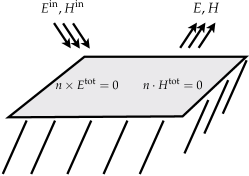
(a) Perfect conductor.

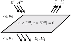
(b) Bi-layered media.

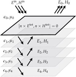
(c) Multi-layered media.

Figure 1: A graphical depiction of the three main categories of planar scattering.

In the case of a perfectly conducting half-space $z\leq 0$, the four physical boundary conditions on the plane $z=0$ are:

$$\boldsymbol{n}\times\boldsymbol{E}^{\text{tot}} =0, \qquad\boldsymbol{n}\cdot\boldsymbol{E}^{\text{tot}} =\rho,$$ (5)

$$\boldsymbol{n}\times\boldsymbol{H}^{\text{tot}} =\boldsymbol{J}, \boldsymbol{n}\cdot\boldsymbol{H}^{\text{tot}} =0,$$

where $\boldsymbol{n}=\hat{\boldsymbol{z}}$ (the unit-normal in the $z$-direction) and $\boldsymbol{J}$, $\rho$ are the physical current and charge, respectively. Depending on the representation of $\boldsymbol{E}$, $\boldsymbol{H}$, one or more of the above boundary conditions may be enforced, or a complex linear combination of multiple conditions may be used. Using the standard representation of $\boldsymbol{E}$ and $\boldsymbol{H}$ in the Lorenz gauge,

$$\boldsymbol{E}(\boldsymbol{x}) =i\omega\mu\int g_{k}(\boldsymbol{x},\boldsymbol{x}^{\prime})\,\boldsymbol{J}(\boldsymbol{x}^{\prime})\,dV^{\prime}-\frac{1}{i\omega\epsilon}\nabla\int g_{k}(\boldsymbol{x},\boldsymbol{x}^{\prime})\,\nabla\cdot\boldsymbol{J}(\boldsymbol{x}^{\prime})\,dV^{\prime},$$ (6)

$$\boldsymbol{H}(\boldsymbol{x}) =\nabla\times\int g_{k}(\boldsymbol{x},\boldsymbol{x}^{\prime})\,\boldsymbol{J}(\boldsymbol{x}^{\prime})\,dV^{\prime},$$

conditions on the tangential fields lead to the electric field integral equation (EFIE) or the magnetic field integral equation (MFIE). Above, $g_{k}$ is the Green’s function for the three-dimensional Helmholtz equation with parameter $k$. The EFIE is a hypersingular integral equation for the current $\boldsymbol{J}$ which can be regularizedContopanagos et al. (2002) via Calderon projections, but still suffers from low-frequency breakdown. The MFIE is stable on simply-connected geometries as $\omega\to 0$Epstein et al. (2013), but for sufficiently small $\omega$ the electric field cannot be recovered without solving an additional integral equationVico et al. (2013). Complex linear combinations of the EFIE and the MFIE yield the combined-field integral equation (CFIE), which is free from spurious resonances in $k$, however still susceptible to instabilities for small $\omega$Song and Chew (1995). It is assumed that the scattered field from a perfectly conducting half-space adheres to the usual Silver-Müller radiation condition - this can be seen from an analysis of the domain Green’s function (which is analytically given in Section III).

In the case of layered dielectric materials, the physical transmission boundary conditions between layers can be phrased in terms of continuity in the tangential components of $\boldsymbol{E}^{\text{tot}}$, $\boldsymbol{H}^{\text{tot}}$, or in the normal components or normal derivatives of $\epsilon\boldsymbol{E}^{\text{tot}}$, $\mu\boldsymbol{H}^{\text{tot}}$:

$$[\boldsymbol{n}\times\boldsymbol{E}^{\text{tot}}] =0, \qquad[\boldsymbol{n}\cdot\epsilon\boldsymbol{E}^{\text{tot}}] =0, \qquad\left[\boldsymbol{n}\cdot\epsilon\frac{\partial\boldsymbol{E}^{\text{tot}}}{\partial n}\right] =0,$$ (7)

$$[\boldsymbol{n}\times\boldsymbol{H}^{\text{tot}}] =0, [\boldsymbol{n}\cdot\mu\boldsymbol{H}^{\text{tot}}] =0, \left[\boldsymbol{n}\cdot\mu\frac{\partial\boldsymbol{H}^{\text{tot}}}{\partial n}\right] =0.$$

The notation $[f]$ is used to denote the discontinuity in $f$ across the boundary. We use this notation as it is convenient for multiple layers. The usual formulation of dielectric problems under these boundary conditions is due to MüllerMüller (1969), which enforces the tangential boundary conditions. This formulation, however, still suffers from numerical instabilities as $\omega\to 0$ due to the integral representation that is usedEpstein, Greengard, and O’Neil (2013a). In layered media problems, the radiation condition imposed on the scattered field is somewhat different than that in free-space, the Silver-Müller condition. The proper radiation condition can be derived from an asymptotic analysis of the domain Green’s functionDurán, Muga, and Nédélec (2009). It suffices to point out that if the dielectrics are slightly absorbing, i.e. have a wavenumber $k_{j}$ with small imaginary part, then non-decaying surface waves are prohibited. Integral equation formulations of the two previous problems on bounded domains have been updated using generalized Debye source representations, which are immune from low-frequency breakdown, topological breakdown (in multiply connected geometries), and spurious resonances in $k$Epstein and Greengard (2010); Epstein, Greengard, and O’Neil (2013a).

So far, we have ignored the topic of discretization. Generally, it is not feasible to use the physical variables $\boldsymbol{J}$ and $\rho$ to discretize the infinite interfaces between homogeneous dielectrics, a prohibitively large linear system would be the result. Therefore, there are two main approaches to the problem: construct the domain Green’s function which accounts for all the boundary conditions between layers, or discretize the Fourier transform of the unknowns defined on the interfaces, which will be numerically compactly supported if the original unknown is smooth. This, latter, spectral approach was introduced by SommerfeldSommerfeld (1909).

In the case of the perfectly conducting half-space or bi-layer dielectric, the dyadic Green’s function can be readily constructedCai (2013); Lindell and Alanen (1984a, b), although possibly taking on a complicated analytical or integral form. In the presence of multiple dielectric layers, no analytic closed-form solution for the Green’s function exists. In fact, the true Green’s function corresponds to the Green’s function for a one-dimensional wave equation with non-constant (piecewise-constant in our case) coefficientsChew (1990). Constructing an analytical approximation or a convergent numerical scheme has been the subject of countless classical electromagnetics and electrical engineering papers.

It should be mentioned that one analytical solution does exist, that of scattering in layered media by pure plane waves (transverse waves). The evaluation of the scattered field can be reduced to recursively calculating reflection and transmission coefficients layer by layerChew (1990). This approach can handle several real-world scattering problems, but is not suitable for arbitrary incoming fields or being embedded inside simulations involving complicated geometry. For example, if the incoming field is generated by dipoles, the spectral components of the field must first be calculated in order for the method of reflection/transmission of plane waves to be applied.

On the other hand, Fourier methods, commonly referred to as Sommerfeld methods, are applicable in the presence of arbitrarily smooth incoming fields. These methods hinge on the Fourier transform of the Helmholtz Green’s function, which is given by:

$$\frac{1}{8\pi^{3}}\int_{\mathbb{R}^{3}}\frac{e^{ik|\boldsymbol{x}|}}{4\pi|\boldsymbol{x}|}\,e^{-i(\xi x+\eta y+\lambda z)}\,dxdydz=\frac{1}{8\pi^{3}}\frac{1}{\xi^{2}+\eta^{2}+\lambda^{2}-k^{2}}.$$ (8)

If $g_{k}$ is written in terms of it’s Fourier transform, and the $\lambda$ integral is evaluated via contour integrationChew (1990), then we have the following Sommerfeld formula for $g_{k}$:

$$g_{k}(\boldsymbol{x},\boldsymbol{x}^{\prime}) =\frac{e^{ik|\boldsymbol{x}-\boldsymbol{x}^{\prime}|}}{4\pi|\boldsymbol{x}-\boldsymbol{x}^{\prime}|}$$ (9)

$$=\frac{1}{8\pi^{3}}\int_{\mathbb{R}^{3}}\frac{e^{i(\xi(x-x^{\prime})+\eta(y-y^{\prime})+\lambda(z-z^{\prime}))}}{{\xi^{2}+\eta^{2}+\lambda^{2}-k^{2}}}\,d\xi d\eta d\lambda$$

$$=\frac{1}{8\pi^{2}}\int_{\mathbb{R}^{2}}\frac{e^{-\sqrt{\xi^{2}+\eta^{2}-k^{2}}|z-z^{\prime}|}}{\sqrt{\xi^{2}+\eta^{2}-k^{2}}}e^{i(\xi(x-x^{\prime})+\eta(y-y^{\prime}))}\,d\xi\,d\eta.$$

In the following sections, we will denote by $\widehat{f}=\mathcal{F}[f]$ the two-dimensional Fourier transform of a function $f$. Using this notation, $\widehat{g}_{k}$ is given by:

$$\widehat{g}_{k}(\xi,\eta,z) =\mathcal{F}[g_{k}]$$ (10)

$$=\frac{1}{8\pi^{2}}\frac{e^{-\sqrt{\xi^{2}+\eta^{2}-k^{2}}|z|}}{\sqrt{\xi^{2}+\eta^{2}-k^{2}}}.$$

The methods described in Sections IV and V do not construct the domain Green’s function directly, but rather rely on Sommerfeld representations of the Helmholtz Green’s function. Unfortunately, these methods result in slow numerical convergence when the incoming field is generated by a scatterer which is near an interface (due to a slowly converging Fourier transform density, similar to the one in the above formula). Schemes that combine the benefits of Green’s function methods (images) with the rapid convergence of far-field Sommerfeld contributions have been recently developedO’Neil, Greengard, and Pataki (2013).

III The dyadic Green’s functions

One of the most popular tools used in numerical simulations of electromagnetic fields in layered media is the dyadic Green’s function. Evaluations of the dyadic Green’s function due to Hertz current dipole sources (either in real-space or Fourier-space) oriented horizontally and vertically can be linearly combined to construct the response for arbitrarily oriented current sourcesCai (2013); Chew (1990). These techniques have been at the center of a large number of layered media scattering schemes, and are widely applicable in complicated geometries because of the local natural of the Green’s function. Furthermore, they provide one possible solution to the problem of scattering from objects which are arbitrarily close to dielectric-dielectric or dielectric-perfectly conducting interfaces as the induced field singularity can be explicitly handled using an adaptive discretization scheme. However, the approach is not without its drawbacks - namely, evaluation of electric fields via convolution of the dyadic Green’s function with a current source becomes numerically unstable as $\omega\to 0$. Evaluation of the dyadic Green’s function requires differentiation followed by division by $\omega^{2}$.

The nature of this low-frequency instability is the same as that which is present in the standard representation of $\boldsymbol{E}$ in the Lorenz gauge, given in equation (6). Unless the divergence of the electric current is handled analytically, with an explicit factoring out of $\omega$, accuracy will be lost in the evaluation of the scalar potential term since the resulting calculation suffers from catastrophic cancellation since $\nabla\cdot\boldsymbol{J}\sim\mathcal{O}(\omega)$. The spectral (Sommerfeld) form of the dyadic Green’s function suffers from the same form of numerical difficulties. Methods which are based on so-called charge-current formulations are one attempt to circumvent this instabilityTaskinen and Yla-Oijala (2006); Vico et al. (2013); Qian and Chew (2009).

The dyadic Green’s function for the electric field in Maxwell’s equations Bladel (1964); Chew (1990) is given by

$$\bar{\boldsymbol{G}}^{E}(\boldsymbol{x},\boldsymbol{x}^{\prime}) =\left(\bar{\boldsymbol{I}}+\frac{1}{k^{2}}\nabla\nabla\right)\frac{e^{ik|\boldsymbol{x}-\boldsymbol{x}^{\prime}|}}{4\pi|\boldsymbol{x}-\boldsymbol{x}^{\prime}|}$$ (11)

$$=\frac{1}{k^{2}}\nabla\times\nabla\times\left(\frac{e^{ik|\boldsymbol{x}-\boldsymbol{x}^{\prime}|}}{4\pi|\boldsymbol{x}-\boldsymbol{x}^{\prime}|}\bar{\boldsymbol{I}}\right),$$

where a dyad $\bar{\boldsymbol{D}}$ can be viewed as either a $3\times 3$ matrix or a rank-two tensor, and the matrix $\nabla\nabla$ has entries $\left(\nabla\nabla\right)_{ij}=\partial^{2}/\partial x_{i}\partial x_{j}$. Likewise, the dyadic Green’s function for the magnetic field is:

$$\bar{\boldsymbol{G}}^{H}(\boldsymbol{x},\boldsymbol{x}^{\prime}) =\frac{1}{i\omega\mu}\nabla\times\bar{\boldsymbol{G}}^{E}_{k}(\boldsymbol{x},\boldsymbol{x}^{\prime})$$ (12)

$$=\frac{1}{i\omega\mu}\nabla\times\bar{\boldsymbol{I}}\frac{e^{ik|\boldsymbol{x}-\boldsymbol{x}^{\prime}|}}{4\pi|\boldsymbol{x}-\boldsymbol{x}^{\prime}|}.$$

For a localized distribution of electric current $\boldsymbol{J}$ in a homogeneous region $V$, the induced electric and magnetic fields are given by

$$\boldsymbol{E}(\boldsymbol{x}) =i\omega\mu\int_{V}\bar{\boldsymbol{G}}^{E}(\boldsymbol{x},\boldsymbol{x}^{\prime})\cdot\boldsymbol{J}(\boldsymbol{x}^{\prime})\,dV_{x^{\prime}},$$ (13)

$$\boldsymbol{H}(\boldsymbol{x}) =i\omega\mu\int_{V}\bar{\boldsymbol{G}}^{H}(\boldsymbol{x},\boldsymbol{x}^{\prime})\cdot\boldsymbol{J}(\boldsymbol{x}^{\prime})\,dV_{x^{\prime}}.$$

The Green’s function for the perfectly conducting half-space can be constructed explicitly via imagesJin (2010) in the lower half-space,

$$\bar{\boldsymbol{G}}^{E}_{\text{pec}}(\boldsymbol{x},\boldsymbol{x}^{\prime})=\bar{\boldsymbol{G}}^{E}(\boldsymbol{x},\boldsymbol{x}^{\prime})-\bar{\boldsymbol{G}}^{E}(\boldsymbol{x},\boldsymbol{x}_{i}^{\prime})+2\bar{\boldsymbol{G}}^{E}(\boldsymbol{x},\boldsymbol{x}_{i}^{\prime})\cdot\hat{\boldsymbol{z}}\hat{\boldsymbol{z}}$$ (14)

where the image points are given by $\boldsymbol{x}_{i}^{\prime}=(x,y,-z)$. The images in the above formula annihilate the tangential components of the electric field on $z=0$. In the presence of planar layered media, the dyadic Green’s function for the electric field must satisfy the variable-coefficient vector wave equation:

$$\left(\nabla\times\frac{1}{\mu(z)}\nabla\times\bar{\boldsymbol{I}}-\omega^{2}\epsilon(z)\bar{\boldsymbol{I}}\right)\bar{\boldsymbol{G}}^{E}(\boldsymbol{x},\boldsymbol{x}^{\prime})=\frac{1}{\mu(z)}\bar{\boldsymbol{I}}\delta(\boldsymbol{x}-\boldsymbol{x}^{\prime}).$$ (15)

A solution in the Fourier domain can be found to this equation using vector wave functions (the vector version of partial wave expansions for the Helmholtz equation, analogous to vector spherical harmonics), but the result requires several calculations and would detract from the following discussion. An expression for the dyadic Green’s function using discrete real-images, like those in equation (14) does not exist. See Section 7.4.2 in ChewChew (1990) for a thorough discussion of the above. Unfortunately, both the physical and the spectral representation of the dyadic Green’s function suffers from low-frequency breakdown; both include division by $k$ or $k^{2}$. Note that the magnetic field dyadic Green’s function does not suffer from low-frequency breakdown, which is obvious from the behavior of the magnetic field integral equation as $\omega\to 0$Cools et al. (2009) (however, other, topological instabilities do arise). The component-wise spectral representation of $\bar{\boldsymbol{G}}^{E}$ is given by:

$$\widehat{\bar{G}_{jk}^{E}}=\frac{1}{8\pi^{2}}\int_{\mathbb{R}^{2}}\left(\delta_{jk}+\frac{1}{k^{2}}\frac{\partial^{2}}{\partial x_{j}\partial x_{k}}\right)\frac{e^{-\sqrt{\xi^{2}+\eta^{2}-k^{2}}|x_{3}-x_{3}^{\prime}|}}{\sqrt{\xi^{2}+\eta^{2}-k^{2}}}\,e^{i(\xi(x_{1}-x_{1}^{\prime})+\eta(x_{3}-x_{3}^{\prime}))}\,d\xi d\eta,$$ (16)

where $(x,y,z)=(x_{1},x_{2},x_{3})$ for the sake of convenient notation. We now move onto the first of our new, stable representations of electromagnetic fields in planar geometries, an extension of the spherical Lorenz-Debye-Mie representation.

IV Planar Mie scattering

The analytical Mie series solution to scattering from perfectly conducting and dielectric spheres is a classic result in mathematical physics due to Mie in 1908Mie (1908), and then shortly thereafter rederived by Debye while working on light pressure in 1909Debye (1909). It is the Mie series solution that is often used to determine whether time-harmonic or fully time-dependent electromagnetic scattering codes are converging to the correct answer at the correct rateChew (1990).

The spherical representation of such solutions is now referred to as the Lorenz-Mie-Debye representation of time-harmonic electromagnetic waves, and is given by:

$$\boldsymbol{E} =\nabla\times\nabla\times(u\,\hat{\boldsymbol{r}})+i\omega\mu\nabla\times(v\,\hat{\boldsymbol{r}}),$$ (17)

$$\boldsymbol{H} =\nabla\times\nabla\times(v\,\hat{\boldsymbol{r}})-i\omega\epsilon\nabla\times(u\,\hat{\boldsymbol{r}}),$$

where $u$ and $v$ are any two scalar functions which satisfy the homogeneous Helmholtz equation with parameter $k$ and $\hat{\boldsymbol{r}}$ is the unit vector in the radial direction. It has been shown several timesPapas (1988); Bouwkamp and Casimir (1954); Wilcox (1957) that knowledge of $E_{r}=\hat{\boldsymbol{r}}\cdot\boldsymbol{E}$ and $H_{r}=\hat{\boldsymbol{r}}\cdot\boldsymbol{H}$ (in the volume) uniquely determines all components of $\boldsymbol{E}$, $\boldsymbol{H}$. Furthermore, on a sphere, the boundary value problem

$$\hat{\boldsymbol{r}}\cdot\boldsymbol{E}|_{\partial B}=f,\qquad\hat{\boldsymbol{r}}\cdot\boldsymbol{H}|_{\partial B}=g,$$ (18)

is uniquely solvable if $f$ and $g$ are mean-zero functionsBouwkamp and Casimir (1954). Since both $E_{r}$ and $H_{r}$ satisfy the homogeneous Helmholtz equation, they can be written in terms of a spherical eigenfunction expansion, leading to the Mie series solution for spherical scattering using the above Debye representation of the electromagnetic fields. Briefly, in Mie scattering one usually specifies $u$, $v$ (known as Debye potentials) using spherical partial wave expansions:

$$u(r,\theta,\varphi) =\sum_{n,m}a_{nm}\,\psi_{n}^{m}(r,\theta,\varphi),$$ (19)

$$v(r,\theta,\varphi) =\sum_{n,m}b_{nm}\,\psi_{n}^{m}(r,\theta,\varphi),$$

where $\psi_{n}^{m}$ is the spherical partial wave function of degree $n$ and order $m$,

$$\psi_{n}^{m}(r,\theta,\varphi)=h_{n}(kr)\,Y_{n}^{m}(\theta,\varphi),$$ (20)

with $h_{n}$ the order $n$ spherical Hankel function of the first kind, and $Y_{n}^{m}$ the spherical harmonic of degree $n$ and order $m$, normalized so that $||Y_{n}^{m}||_{2}=1$. Using the coefficients $a^{\text{in}}_{nm}$, $b^{\text{in}}_{nm}$ of a similarly expressed incoming electromagnetic field, one can match modes depending on the boundary conditions and analytically calculate $a_{nm}$, $b_{nm}$Papas (1988); Bouwkamp and Casimir (1954); Wilcox (1957); Gimbutas and Greengard (2013) for the scattered field. The series for $u$, $v$ can be truncated depending on the number of partial wave function needed to describe the incoming field.

We now extend the above spherical representation of Maxwell fields to one which is immune from low-frequency breakdown and compatible with planar geometries. In Cartesian coordinates, it is easy to show uniqueness of Maxwell fields which obey the Silver-Müller radiation condition given $E_{z}=\hat{\boldsymbol{z}}\cdot\boldsymbol{E}$ and $H_{z}=\hat{\boldsymbol{z}}\cdot\boldsymbol{H}$. For if $E_{z}=0$, $H_{z}=0$, the only electromagnetic fields satisfying Maxwell’s equations must be of the form:

$$\boldsymbol{E} =ae^{ikz}\hat{\boldsymbol{x}}+be^{ikz}\hat{\boldsymbol{y}},$$ (21)

$$\boldsymbol{H} =-be^{ikz}\hat{\boldsymbol{x}}+ae^{ikz}\hat{\boldsymbol{y}},$$

where $\hat{\boldsymbol{x}}$, $\hat{\boldsymbol{y}}$ are unit vectors in the $x$ and $y$ directions, respectively, and $a$, $b$ are constants. However, these fields do not decay at infinity. Therefore, the coefficients $a$, $b$ must be set to zero in order for the field to obey the Silver-Müller radiation condition. Furthermore, if the electromagnetic fields are generated by a finite collection of current, $\boldsymbol{J}$, located in a volume $V$, then the $z$-components can be calculated easily using the Lorenz gauge representation of fields, as in (6). The resulting expression is analogous to that derived by Bouwkamp and CasimirBouwkamp and Casimir (1954) for the radial components, so we omit it here. In order to extend their spherical result to the upper half-space, we change representation (19) slightly. It is clear that another valid representation of Maxwell fields for $z>0$ is given by

$$\boldsymbol{E} =\nabla\times\nabla\times(u\,\hat{\boldsymbol{z}})+i\omega\mu\nabla\times(v\,\hat{\boldsymbol{z}}),$$ (22)

$$\boldsymbol{H} =\nabla\times\nabla\times(v\,\hat{\boldsymbol{z}})-i\omega\epsilon\nabla\times(u\,\hat{\boldsymbol{z}}),$$

where the radial unit vector $\hat{\boldsymbol{r}}$ has been replaced with the unit vector in the $z$-direction, $\hat{\boldsymbol{z}}$. It is easy to show a direct correspondence between $u$, $v$ and the $z$-components of the electromagnetic field:

$$E_{z}(x,y,z)=-\left(\frac{\partial^{2}}{\partial x^{2}}+\frac{\partial^{2}}{\partial y^{2}}\right)u(x,y,z),\qquad H_{z}(x,y,z)=-\left(\frac{\partial^{2}}{\partial x^{2}}+\frac{\partial^{2}}{\partial y^{2}}\right)v(x,y,z).$$ (23)

In order to write $u$, $v$ in terms of the driving current $\boldsymbol{J}$, which is now assumed to lie in a volume $V$ located in the lower half-space, instead of expressing $u$, $v$ as partial wave expansions it is convenient to form them in a manner which is compatible with the planar geometry of the problem while still automatically satisfying the Helmholtz equation. For some $\widehat{\sigma}=\mathcal{F}[\sigma]$, $\widehat{\tau}=\mathcal{F}[\tau]$, we assume that $u$, $v$ are generally of the form:

$$u(x,y,z) =\int_{\mathbb{R}^{2}}g_{k}(x,y,z)\,\sigma(x,y)\,dxdy$$ (24)

$$=\int_{\mathbb{R}^{2}}\widehat{g}_{k}(\xi,\eta,z)\,\widehat{\sigma}(\xi,\eta)\,e^{i(\xi x+\eta y)}\,d\xi d\eta,$$

$$v(x,y,z) =\int_{\mathbb{R}^{2}}\widehat{g}_{k}(\xi,\eta,z)\,\widehat{\tau}(\xi,\eta)\,e^{i(\xi x+\eta y)}\,d\xi d\eta,$$

where $\widehat{g}_{k}$ is the Fourier transform of the three-dimensional Helmholtz Green’s function, given in formula (9). Using this representation, $u$ and $v$ can be thought of as a superposition of plane waves that obey the Sommerfeld radiation condition for the Helmholtz equation. Substituting the spectral Sommerfeld formula for $g_{k}$ into the Lorenz gauge representation of $\boldsymbol{H}$ in (6), we see that

$$\boldsymbol{H}(\boldsymbol{x}) =\nabla\times\int_{V}\left(\frac{1}{8\pi^{2}}\int_{\mathbb{R}^{2}}\frac{e^{-\sqrt{\xi^{2}+\eta^{2}-k^{2}}(z-z^{\prime})}}{\sqrt{\xi^{2}+\eta^{2}-k^{2}}}\,e^{i(\xi(x-x^{\prime})+\eta(y-y^{\prime}))}\,d\xi d\eta\right)\boldsymbol{J}(\boldsymbol{x}^{\prime})\,dV^{\prime}$$ (25)

$$=\nabla\times\int_{\mathbb{R}^{2}}\widehat{g}_{k}(\xi,\eta,z)\left(\int_{V}e^{\sqrt{\xi^{2}+\eta^{2}-k^{2}}z^{\prime}}\,\boldsymbol{J}(\boldsymbol{x}^{\prime})e^{-i(\xi x^{\prime}+\eta y^{\prime})}dV^{\prime}\right)e^{i(\xi x+\eta y)}\,d\xi d\eta.$$

This formula can be interpreted as constructing $\boldsymbol{H}$ from a superposition of attenuated transverse two-dimensional Fourier transforms of the current $\boldsymbol{J}$. The normal component $H_{z}$ is then given by

$$H_{z}(\boldsymbol{x})=\int_{\mathbb{R}^{2}}\widehat{g}_{k}(\xi,\eta,z)\left(\int_{V}e^{\sqrt{\xi^{2}+\eta^{2}-k^{2}}z^{\prime}}\,\left[i\xi J_{y}(\boldsymbol{x}^{\prime})-i\eta J_{x}(\boldsymbol{x}^{\prime})\right]e^{-i(\xi x^{\prime}+\eta y^{\prime})}\,dV^{\prime}\right)e^{i(\xi x+\eta y)}\,d\xi d\eta.$$ (26)

Similarly, an expression for $\boldsymbol{E}$ can be derived. We only provide the formula for $E_{z}$, and not the derivation:

$$E_{z}(\boldsymbol{x})=\int_{\mathbb{R}^{2}}\widehat{g}_{k}(\xi,\eta,z)\left(\int_{V}e^{\beta z^{\prime}}\,\left[i\omega\mu J_{z}(\boldsymbol{x}^{\prime})+\frac{\beta}{\epsilon}\,\rho(\boldsymbol{x}^{\prime})\right]\,e^{-i(\xi x^{\prime}+\eta y^{\prime})}\,dV^{\prime}\right)\,e^{i(\xi x+\eta y)}\,d\xi d\eta,$$ (27)

where $\beta=\sqrt{\xi^{2}+\eta^{2}-k^{2}}$ and we have used the consistency condition $\nabla\cdot\boldsymbol{J}=i\omega\rho$. Substituting these expressions into relation (23), and using representation (24) for $u$, $v$, we see that $\widehat{\sigma}$ and $\widehat{\tau}$ are formally given by

$$\widehat{\sigma}(\xi,\eta) =\frac{1}{\xi^{2}+\eta^{2}}\,\int_{V}e^{\sqrt{\xi^{2}+\eta^{2}-k^{2}}z^{\prime}}\,\left[i\omega\mu J_{z}(\boldsymbol{x}^{\prime})+\frac{\sqrt{\xi^{2}+\eta^{2}-k^{2}}}{\epsilon}\,\rho(\boldsymbol{x}^{\prime})\right]\,e^{-i(\xi x^{\prime}+\eta y^{\prime})}\,dV^{\prime},$$ (28)

$$\widehat{\tau}(\xi,\eta) =\frac{1}{\xi^{2}+\eta^{2}}\int_{V}e^{\sqrt{\xi^{2}+\eta^{2}-k^{2}}z^{\prime}}\,\left[i\xi J_{y}(\boldsymbol{x}^{\prime})-i\eta J_{x}(\boldsymbol{x}^{\prime})\right]e^{-i(\xi x^{\prime}+\eta y^{\prime})}dV^{\prime}.$$

The integrands in the corresponding formulae for $\boldsymbol{E}$, $\boldsymbol{H}$ are clearly integrable because of the extra $\xi$ and $\eta$ terms introduced by differentiation. Therefore, equations (22), (24), and (28) provide a unique representation of the electromagnetic field in the half-space $z>0$.

We can readily use the above method to calculate the solution of scattering in $z>0$ from the perfect conducting half-space $z\leq 0$ using the boundary condition $\boldsymbol{n}\times\boldsymbol{E}^{\text{tot}}=0$ on $z=0$. Using representation (24) for the Debye potentials and representation (22) for scattered fields $\boldsymbol{E}$, $\boldsymbol{H}$, the components of $\boldsymbol{E}$ on $z=0$ can be calculated as

$$E_{x}(x,y,0) =\int_{\mathbb{R}^{2}}\widehat{g}_{k}(\xi,\eta,0)\,\left(i\xi\,\sqrt{\xi^{2}+\eta^{2}-k^{2}}\,\widehat{\sigma}(\xi,\eta)-\omega\mu\eta\,\widehat{\tau}(\xi,\eta)\right)e^{i(\xi x+\eta y)}\,d\xi d\eta,$$ (29)

$$E_{y}(x,y,0) =\int_{\mathbb{R}^{2}}\widehat{g}_{k}(\xi,\eta,0)\,\left(i\eta\,\sqrt{\xi^{2}+\eta^{2}-k^{2}}\,\widehat{\sigma}(\xi,\eta)+\omega\mu\xi\,\widehat{\tau}(\xi,\eta)\right)\,e^{i(\xi x+\eta y)}\,d\xi d\eta,$$

$$E_{z}(x,y,0) =\int_{\mathbb{R}^{2}}\widehat{g}_{k}(\xi,\eta,0)\,\left(\xi^{2}+\eta^{2}\right)\,\widehat{\sigma}(\xi,\eta)\,e^{i(\xi x+\eta y)}\,d\xi d\eta.$$

Enforcing the boundary condition $\boldsymbol{n}\times\boldsymbol{E}^{\text{tot}}=0$ yields a two-by-two linear system for $\widehat{\sigma}(\xi,\eta)$, $\widehat{\tau}(\xi,\eta)$:

$$\widehat{g}_{k}(\xi,\eta,0)\left(i\xi\,\sqrt{\xi^{2}+\eta^{2}-k^{2}}\,\widehat{\sigma}(\xi,\eta)-\omega\mu\eta\,\widehat{\tau}(\xi,\eta)\right) =-\widehat{E}^{\text{in}}_{x}(\xi,\eta),$$ (30)

$$\widehat{g}_{k}(\xi,\eta,0)\left(i\eta\,\sqrt{\xi^{2}+\eta^{2}-k^{2}}\,\widehat{\sigma}(\xi,\eta)+\omega\mu\xi\,\widehat{\tau}(\xi,\eta)\right) =-\widehat{E}^{\text{in}}_{y}(\xi,\eta).$$

The functions $\widehat{\sigma}$ and $\widehat{\tau}$ are then formally given as

$$\widehat{\sigma}(\xi,\eta) =\frac{8\pi^{2}i}{\xi^{2}+\eta^{2}}\left(\xi\widehat{E}^{\text{in}}_{x}(\xi,\eta))+\eta\widehat{E}^{\text{in}}_{y}(\xi,\eta)\right),$$ (31)

$$\widehat{\tau}(\xi,\eta) =\frac{8\pi^{2}\,\sqrt{\xi^{2}+\eta^{2}-k^{2}}}{\omega\mu(\xi^{2}+\eta^{2})}\left(\eta\widehat{E}^{\text{in}}_{y}(\xi,\eta))-\xi\widehat{E}^{\text{in}}_{x}(\xi,\eta)\right),$$

where we have explicitly substituted in the expression for $\widehat{g}_{k}$. It is interesting to point out that the terms $\xi\widehat{E}^{\text{in}}_{x}+\eta\widehat{E}^{\text{in}}_{y}$ and $\eta\widehat{E}^{\text{in}}_{x}-\xi\widehat{E}^{\text{in}}_{y}$ are proportional to the Fourier transforms of the surface divergence and surface curl of the incoming field $\boldsymbol{E}^{\text{in}}$. This is not surprising considering that non-physical currents used in the generalized Debye representation are constructed from surface gradients and surface curls on arbitrary smooth geometries; see the following section for a brief introduction to this formulation.

If the incoming field $\boldsymbol{E}^{\text{in}}$, $\boldsymbol{H}^{\text{in}}$ is not known in terms of its Fourier transform, but rather in terms of its Mie series or component-wise partial wave expansion, then its Fourier transform can be calculated analytically using the identities found in the appendix of this note. Numerical schemes based on this observation are currently being developed.

Generalizing the above approach to layered media geometries is relatively straightforward, requiring several Fourier calculations and matching of boundary conditions. It should be noted that no low-frequency breakdown occurs in the resulting formulas for $\boldsymbol{E}$, $\boldsymbol{H}$. This approach provides one alternative to the use of the dyadic Green’s function. We skip the layered media calculation and instead turn our attention to generalized Debye source methods in half-spaces and layered media geometries.

V Generalized Debye sources

The generalized Debye source representation of time-harmonic electromagnetic wavesEpstein and Greengard (2010); Epstein, Greengard, and O’Neil (2013a) is designed to provide a unified framework for the representation of solutions to Maxwell’s equations in smooth geometries of arbitrary connectedness. The resulting representations lead to well-conditioned, resonance-free second-kind integral equations which are immune from low-frequency and topological breakdownCools et al. (2009); Epstein et al. (2013). In general, for a simply-connected bounded scatterer $\Omega$ with boundary $\Gamma$, the scattered fields $\boldsymbol{E}$ and $\boldsymbol{H}$ are constructed from mean-zero scalar sources $r$, $q$ on $\Gamma$ using the fully symmetric potential/anti-potential representation:

$$\boldsymbol{E} =\sqrt{\mu}\left(ik\boldsymbol{A}-\nabla\varphi-\nabla\times\boldsymbol{Q}\right),$$ (32)

$$\boldsymbol{H} =\sqrt{\epsilon}\left(ik\boldsymbol{Q}-\nabla\psi+\nabla\times\boldsymbol{A}\right),$$

where $\boldsymbol{A}$, $\boldsymbol{Q}$, $\varphi$, and $\psi$ are functions defined by the single-layer potentials

$$\boldsymbol{A}(\boldsymbol{x}) =\int_{\Gamma}g_{k}(\boldsymbol{x},\boldsymbol{x}^{\prime})\,\boldsymbol{j}(\boldsymbol{x}^{\prime})\,da_{x^{\prime}}, \qquad\boldsymbol{Q}(\boldsymbol{x}) =\int_{\Gamma}g_{k}(\boldsymbol{x},\boldsymbol{x}^{\prime})\,\boldsymbol{m}(\boldsymbol{x}^{\prime})\,da_{x^{\prime}},$$ (33)

$$\varphi(\boldsymbol{x}) =\int_{\Gamma}g_{k}(\boldsymbol{x},\boldsymbol{x}^{\prime})\,r(\boldsymbol{x}^{\prime})\,da_{x^{\prime}}, \psi(\boldsymbol{x}) =\int_{\Gamma}g_{k}(\boldsymbol{x},\boldsymbol{x}^{\prime})\,q(\boldsymbol{x}^{\prime})\,da_{x^{\prime}}.$$

From now on, the Helmholtz single-layer potential with kernel $g_{k}$ of function $f$ will be denoted as $\mathcal{S}_{k}f$. The functions $r$ and $q$ are known as generalized Debye sources. In order for $\boldsymbol{E}$ and $\boldsymbol{H}$ in equation (32) to satisfy Maxwell’s equations, the tangential vector fields $\boldsymbol{j}$, $\boldsymbol{m}$ and scalar functions $r$, $q$ must satisfy the consistency conditions

$$\nabla_{\Gamma}\cdot\boldsymbol{j}=ikr,\qquad\nabla_{\Gamma}\cdot\boldsymbol{m}=ikq,$$ (34)

where $\nabla_{\Gamma}\cdot$ is the surface divergence. Depending on the boundary conditions, $\boldsymbol{j}$ and $\boldsymbol{m}$ are explicitly constructed from $r$ and $q$ such that that above consistency conditions are automatically satisfied, as well as to ensure that the representation is unique (i.e. no spurious resonances in the resulting integral equations). For example, in the case where $\Omega$ is a simply-connected, bounded perfect electric conductor ($\boldsymbol{n}\times\boldsymbol{E}^{\text{tot}}=0$ and $\boldsymbol{n}\cdot\boldsymbol{H}^{\text{tot}}=0$) the tangential fields $\boldsymbol{j}$ and $\boldsymbol{m}$ are constructed as:

$$\boldsymbol{j} =ik\left(\nabla_{\Gamma}\triangle^{-1}_{\Gamma}r-\boldsymbol{n}\times\nabla_{\Gamma}\triangle^{-1}_{\Gamma}q\right),$$ (35)

$$\boldsymbol{m} =\boldsymbol{n}\times\boldsymbol{j},$$

where $\nabla_{\Gamma}$ is the surface gradient and $\triangle^{-1}_{\Gamma}$ is the inverse of the surface Laplacian restricted to mean-zero functions. When the boundary $\Gamma$ is multiply connected, extra circulation conditions must be added to the boundary conditions in order to determine the projection of $\boldsymbol{j}$ and $\boldsymbol{m}$ onto the space of harmonic vector fields along $\Gamma$Epstein and Greengard (2010); Epstein, Greengard, and O’Neil (2013a). We will skip this discussion here, as it has been previously detailed in other papers by the author, and is irrelevant in light of the unbounded planar geometries to be addressed. In order to determine $r$, $q$, we enforce two scalar conditions on the surface of the conductor instead of one vector condition. These scalar conditions are given by:

$$\mathcal{S}_{0}\nabla_{\Gamma}\cdot\boldsymbol{n}\times\boldsymbol{E}^{\text{tot}}=0,\qquad\text{and}\qquad\boldsymbol{n}\cdot\boldsymbol{H}^{\text{tot}}=0.$$ (36)

Using these scalar boundary conditions, representations which guarantee uniqueness and which lead to second-kind integral equations for $r$ and $q$ that are free from low-frequency breakdown and spurious resonances have been derived for the perfect electric conductorEpstein and Greengard (2010) and the dielectric transmission problemEpstein, Greengard, and O’Neil (2013a). The generalized Debye source representation also has the feature that $\boldsymbol{E}$ and $\boldsymbol{H}$ gracefully decouple as $\omega\to 0$, leaving only the scalar potential terms in simply connected geometries - $\boldsymbol{E}$ depends only on $r$ and $\boldsymbol{H}$ depends only on $q$. This can be viewed as a generalization of the spherical Lorenz-Mie-Debye representation.

V.1 Generalized Debye sources on a perfectly conducting half-space

We will now derive a Sommerfeld-like formula for scattering from a perfectly conducting half-space $z\leq 0$ which is immune from low-frequency breakdown, and decouples $\boldsymbol{E}$ and $\boldsymbol{H}$ for any value of $\omega$. This requires extending the generalized Debye source representation to the domain $z>0$. In this geometry, the representation simplifies in that the surface differential operators reduce to their two-dimensional Cartesian counterparts, $\nabla$, $\nabla\cdot$, and $\triangle$. We first express the scalar densities $r$ and $q$ in terms of their Fourier transform on the $xy$-plane:

$$r(x,y)=\int_{\mathbb{R}^{2}}\widehat{r}(\xi,\eta)\,e^{i(x\xi+y\eta)}\,d\xi d\eta,\qquad q(x,y)=\int_{\mathbb{R}^{2}}\widehat{q}(\xi,\eta)\,e^{i(x\xi+y\eta)}\,d\xi d\eta,$$ (37)

where it is implied that the mean-zero condition is satisfied via $\widehat{r}(0,0)=\widehat{q}(0,0)=0$. In the case of the perfect conductor, it now suffices to calculate the values of the two scalar boundary operators, $\mathcal{S}_{0}\nabla\cdot\boldsymbol{E}$ and $\boldsymbol{n}\cdot\boldsymbol{H}$, where from now on we will abbreviate:

$$\mathcal{S}_{0}\nabla\cdot\boldsymbol{E}=-\mathcal{S}_{0}\nabla\cdot\boldsymbol{n}\times\boldsymbol{n}\times\boldsymbol{E},$$ (38)

that is, we apply $\mathcal{S}_{0}\nabla\cdot$ to the tangential projection of $\boldsymbol{E}$. All operators in the generalized Debye source representation are differential or convolutional; by writing the Helmholtz equation’s Green’s function in its Sommerfeld representation all operators diagonalize and can be applied via multiplication. We recall from equation (9) that the Fourier transform $\widehat{g}_{k}$ of the Green’s function for the Helmholtz equation $g_{k}$ is given by:

$$\widehat{g}_{k}(\xi,\eta,z)=\frac{1}{8\pi^{2}}\frac{e^{-\sqrt{\xi^{2}+\eta^{2}-k^{2}}|z|}}{\sqrt{\xi^{2}+\eta^{2}-k^{2}}}.$$ (39)

A single-layer potential of an integral function $f$, $\mathcal{S}_{k}f$, can then be written as

$$\mathcal{S}_{k}[f](\boldsymbol{x})=\int_{\mathbb{R}^{2}}\widehat{g}_{k}(\xi,\eta,z)\,\widehat{f}(\xi,\eta)\,d\xi d\eta.$$ (40)

Evaluation of $\nabla$ and $\nabla\cdot$ are straightforward multiplications by $i\xi$ and $i\eta$, and the inverse surface Laplacian $\triangle^{-1}$ applied to a mean-zero function is given by:

$$\triangle^{-1}[f](x,y)=\int_{\mathbb{R}^{2}}\frac{\widehat{f}(\xi,\eta)}{-\xi^{2}-\eta^{2}}\,e^{i(\xi x+\eta y)}\,d\xi d\eta.$$ (41)

After several tedious calculations, using the above identities and the representations of $\boldsymbol{E}$, $\boldsymbol{H}$ from equation (32), we are able to calculate $\mathcal{S}_{0}\nabla\cdot\boldsymbol{E}$ and $\boldsymbol{n}\cdot\boldsymbol{H}$ as

$$\mathcal{S}_{0}\nabla\cdot\boldsymbol{E} =\sqrt{\mu}\int_{\mathbb{R}^{2}}\left(\xi^{2}+\eta^{2}-k^{2}-ik\sqrt{\xi^{2}+\eta^{2}-k^{2}}\right)\widehat{g}_{0}(\xi,\eta,0)\,\widehat{g}_{k}(\xi,\eta,0)\,\widehat{r}(\xi,\eta)\,d\xi d\eta,$$ (42)

$$\boldsymbol{n}\cdot\boldsymbol{H} =\sqrt{\epsilon}\int_{\mathbb{R}^{2}}\left(\sqrt{\xi^{2}+\eta^{2}-k^{2}}-ik\right)\,\widehat{g}_{k}(\xi,\eta,0)\,\widehat{q}(\xi,\eta)\,d\xi d\eta.$$

The Fourier transforms of $r$ and $q$ can then be calculated as

$$\widehat{r}(\xi,\eta) =-\frac{64\pi^{4}}{\sqrt{\mu}}\mathcal{F}\left[\mathcal{S}_{0}\nabla\cdot\boldsymbol{E}^{\text{in}}\right]\frac{\sqrt{\xi^{2}+\eta^{2}}}{\sqrt{\xi^{2}+\eta^{2}-k^{2}}-ik},$$ (43)

$$\widehat{q}(\xi,\eta) =-\frac{8\pi^{2}}{\sqrt{\epsilon}}\mathcal{F}\left[\boldsymbol{n}\cdot\boldsymbol{H}^{\text{in}}\right]\frac{\sqrt{\xi^{2}+\eta^{2}-k^{2}}}{\sqrt{\xi^{2}+\eta^{2}-k^{2}}-ik},$$

where we have substituted in the expressions for the Green’s functions $\widehat{g}_{k}$ and $\widehat{g}_{0}$. It is clear that in the previous formulas, the equation for $r$ does not depend on the incoming magnetic field $\boldsymbol{H}^{\text{in}}$, and the equation for $q$ does not depend on the incoming electric field $\boldsymbol{E}^{\text{in}}$. The unknowns have effectively been decoupled, which is not surprising because of the well-known separation of the vector wave equations for $\boldsymbol{E}$ and $\boldsymbol{H}$ into transverse electric and transverse magnetic fields. In this respect, the generalized Debye sources are in one-to-one correspondence with transverse electric and magnetic fields in the presence of a perfectly conducting half-space. The expressions for $\widehat{r}$ and $\widehat{q}$ in (43) are stable as $\omega\to 0$, and when $\omega=0$,

$$\widehat{r}(\xi,\eta) =-\frac{64\pi^{4}}{\sqrt{\mu}}\mathcal{F}\left[\mathcal{S}_{0}\nabla\cdot\boldsymbol{E}^{\text{in}}\right],$$ (44)

$$\widehat{q}(\xi,\eta) =-\frac{8\pi^{2}}{\sqrt{\epsilon}}\mathcal{F}\left[\boldsymbol{n}\cdot\boldsymbol{H}^{\text{in}}\right],$$

analogous to the solution of a Neumann problem on a half-space. We now derive similar Fourier-type solutions for scattering in layered media using generalized Debye sources.

V.2 Generalized Debye sources in layered media

We now turn to the calculation of electromagnetic fields in layered media using the generalized Debye source representation. As in the previous section, Section V.1, we will derive formulae for $\boldsymbol{E}$, $\boldsymbol{H}$ which are stable and decouple as the frequency $\omega$ tends to $0$. The simple two-layer case is described first, with the generalization to $n$-layers later. We will see that adjacent layers are coupled through the generalized Debye sources; in the case of several layers, this coupling leads to a banded system of linear equations whose bandwidth is independent of the number of layers.

The calculations of the normal and tangential components of generalized Debye source representations on the boundary of planar layered media are similar to those in the previous section, but in order to ensure uniqueness we require a different construction of the tangential vector fields $\boldsymbol{j}$ and $\boldsymbol{m}$Epstein, Greengard, and O’Neil (2013a). If the dielectric constants for $z>0$ are $\epsilon_{0}$, $\mu_{0}$ and for $z<=0$ are $\epsilon_{1}$, $\mu_{1}$, then we define the wavenumber $k_{j}=\omega\sqrt{\epsilon_{j}\mu_{j}}$. The fields $\boldsymbol{E}_{0}$, $\boldsymbol{H}_{0}$ and $\boldsymbol{E}_{1}$, $\boldsymbol{H}_{1}$ in the upper and lower half-spaces, respectively, are given as

$$\boldsymbol{E}_{j} =\sqrt{\mu_{j}}\left(ik_{j}\mathcal{S}_{k_{j}}[\boldsymbol{j}_{j}]-\nabla\mathcal{S}_{k_{j}}[r_{j}]-\nabla\times\mathcal{S}_{k_{j}}[\boldsymbol{m}_{j}]\right),$$ (45)

$$\boldsymbol{H}_{j} =\sqrt{\epsilon_{j}}\left(ik_{j}\mathcal{S}_{k_{j}}[\boldsymbol{m}_{j}]-\nabla\mathcal{S}_{k_{j}}[q_{j}]+\nabla\times\mathcal{S}_{k_{j}}[\boldsymbol{j}_{j}]\right),$$

where the explicit layer potential dependence is shown instead of using vector potential notation because of the variable wavenumber in the Green’s function. It is worth pointing out that if $z>0$, then

$$\mathcal{S}_{k}[f](\boldsymbol{x})=\frac{1}{8\pi^{2}}\int_{\mathbb{R}^{2}}\frac{e^{-\sqrt{\xi^{2}+\eta^{2}-k^{2}}z}}{\sqrt{\xi^{2}+\eta^{2}-k^{2}}}\,\widehat{f}(\xi,\eta)\,d\xi d\eta,$$ (46)

and if $z<0$,

$$\mathcal{S}_{k}[f](\boldsymbol{x})=\frac{1}{8\pi^{2}}\int_{\mathbb{R}^{2}}\frac{e^{\sqrt{\xi^{2}+\eta^{2}-k^{2}}z}}{\sqrt{\xi^{2}+\eta^{2}-k^{2}}}\,\widehat{f}(\xi,\eta)\,d\xi d\eta.$$ (47)

This is a direct consequence of the spectral formula for the Helmholtz Green’s function. Sign mistakes in the exponent will lead to not only incorrect formulas, but non-convergent integrands. Furthermore, as mentioned above, the tangential vector fields $\boldsymbol{j}_{j}$, $\boldsymbol{m}_{j}$ are constructed slightly differentlyEpstein, Greengard, and O’Neil (2013a) than in the perfectly conducting case, with

$$\boldsymbol{j}_{0} =i\omega\left(\sqrt{\mu_{0}\epsilon_{0}}\nabla\triangle^{-1}r_{0}-\epsilon_{1}\sqrt{\frac{\mu_{1}}{\epsilon_{0}}}\boldsymbol{n}\times\nabla\triangle^{-1}r_{1}\right), \qquad\boldsymbol{j}_{1} =\boldsymbol{n}\times\sqrt{\frac{\epsilon_{0}}{\epsilon_{1}}}\boldsymbol{j}_{0},$$ (48)

$$\boldsymbol{m}_{0} =i\omega\left(\sqrt{\mu_{0}\epsilon_{0}}\nabla\triangle^{-1}q_{0}-\mu_{1}\sqrt{\frac{\epsilon_{1}}{\mu_{0}}}\boldsymbol{n}\times\nabla\triangle^{-1}q_{1}\right), \boldsymbol{m}_{1} =\boldsymbol{n}\times\sqrt{\frac{\mu_{0}}{\mu_{1}}}\boldsymbol{m}_{0}.$$

The consistency conditions that are enforced automatically via the construction of $\boldsymbol{j}_{j}$, $\boldsymbol{m}_{j}$ are, as before,

$$\nabla\cdot\boldsymbol{j}_{j}=ikr_{j},\qquad\nabla\cdot\boldsymbol{m}_{j}=ikq_{j}.$$ (49)

As in the previous section, we now replace the generalized Debye sources $r_{j}$, $q_{j}$ with their Fourier transform representations,

$$r_{j}(x,y)=\int_{\mathbb{R}^{2}}\widehat{r}_{j}(\xi,\eta)\,e^{i(x\xi+y\eta)}\,d\xi d\eta,\qquad q_{j}(x,y)=\int_{\mathbb{R}^{2}}\widehat{q}_{j}(\xi,\eta)\,e^{i(x\xi+y\eta)}\,d\xi d\eta.$$ (50)

The Calderón preconditioned transmission boundary conditions to be enforced on the interfaces areEpstein, Greengard, and O’Neil (2013a):

$$\left[\mathcal{S}_{0}\nabla\cdot\boldsymbol{E}^{\text{tot}}\right] =0,\qquad \left[\boldsymbol{n}\cdot\epsilon\boldsymbol{E}^{\text{tot}}\right] =0,$$ (51)

$$\left[\mathcal{S}_{0}\nabla\cdot\boldsymbol{H}^{\text{tot}}\right] =0, \left[\boldsymbol{n}\cdot\mu\boldsymbol{H}^{\text{tot}}\right] =0.$$

Using these representations, each of the operators can be written in terms of its Fourier transform:

$$\mathcal{F}\left[\mathcal{S}_{0}\nabla\cdot\boldsymbol{E}_{0}\right] =\sqrt{\mu_{0}}\,\widehat{g}_{0}(\xi,\eta,0)\,\widehat{g}_{k_{0}}(\xi,\eta,0)\left(\left(\xi^{2}+\eta^{2}-k_{0}^{2}\right)\,\widehat{r}_{0}(\xi,\eta)-i\omega\mu_{1}\sqrt{\frac{\epsilon_{1}}{\mu_{0}}}\sqrt{\xi^{2}+\eta^{2}-k_{0}^{2}}\,\widehat{q}_{1}(\xi,\eta)\right),$$ (52)

$$\mathcal{F}\left[\mathcal{S}_{0}\nabla\cdot\boldsymbol{E}_{1}\right] =\sqrt{\mu_{1}}\,\widehat{g}_{0}(\xi,\eta,0)\,\widehat{g}_{k_{1}}(\xi,\eta,0)\left(\left(\xi^{2}+\eta^{2}-k_{1}^{2}\right)\,\widehat{r}_{1}(\xi,\eta)+i\omega\mu_{0}\sqrt{\frac{\epsilon_{0}}{\mu_{1}}}\sqrt{\xi^{2}+\eta^{2}-k_{1}^{2}}\,\widehat{q}_{0}(\xi,\eta)\right),$$

$$\mathcal{F}\left[\mathcal{S}_{0}\nabla\cdot\boldsymbol{H}_{0}\right] =\sqrt{\epsilon_{0}}\,\widehat{g}_{0}(\xi,\eta,0)\,\widehat{g}_{k_{0}}(\xi,\eta,0)\left(\left(\xi^{2}+\eta^{2}-k_{0}^{2}\right)\,\widehat{q}_{0}(\xi,\eta)-i\omega\epsilon_{1}\sqrt{\frac{\mu_{1}}{\epsilon_{0}}}\sqrt{\xi^{2}+\eta^{2}-k_{0}^{2}}\,\widehat{r}_{1}(\xi,\eta)\right),$$

$$\mathcal{F}\left[\mathcal{S}_{0}\nabla\cdot\boldsymbol{H}_{1}\right] =\sqrt{\epsilon_{1}}\,\widehat{g}_{0}(\xi,\eta,0)\,\widehat{g}_{k_{1}}(\xi,\eta,0)\left(\left(\xi^{2}+\eta^{2}-k_{1}^{2}\right)\,\widehat{q}_{1}(\xi,\eta)+i\omega\epsilon_{0}\sqrt{\frac{\mu_{0}}{\epsilon_{1}}}\sqrt{\xi^{2}+\eta^{2}-k_{1}^{2}}\,\widehat{r}_{0}(\xi,\eta)\right),$$

$$\mathcal{F}\left[\boldsymbol{n}\cdot\epsilon_{0}\boldsymbol{E}_{0}\right] =\epsilon_{0}\sqrt{\mu_{0}}\,\widehat{g}_{k_{0}}(\xi,\eta,0)\left(\sqrt{\xi^{2}+\eta^{2}-k_{0}^{2}}\,\widehat{r}_{0}(\xi,\eta)+i\omega\mu_{1}\sqrt{\frac{\epsilon_{1}}{\mu_{0}}}\,\widehat{q}_{1}(\xi,\eta)\right),$$

$$\mathcal{F}\left[\boldsymbol{n}\cdot\epsilon_{1}\boldsymbol{E}_{1}\right] =-\epsilon_{1}\sqrt{\mu_{1}}\,\widehat{g}_{k_{1}}(\xi,\eta,0)\left(\sqrt{\xi^{2}+\eta^{2}-k_{1}^{2}}\,\widehat{r}_{1}(\xi,\eta)+i\omega\mu_{0}\sqrt{\frac{\epsilon_{0}}{\mu_{1}}}\,\widehat{q}_{0}(\xi,\eta)\right),$$

$$\mathcal{F}\left[\boldsymbol{n}\cdot\mu_{0}\boldsymbol{H}_{0}\right] =\mu_{0}\sqrt{\epsilon_{0}}\,\widehat{g}_{k_{0}}(\xi,\eta,0)\left(\sqrt{\xi^{2}+\eta^{2}-k_{0}^{2}}\,\widehat{q}_{0}(\xi,\eta)-i\omega\epsilon_{1}\sqrt{\frac{\mu_{1}}{\epsilon_{0}}}\,\widehat{r}_{1}(\xi,\eta)\right),$$

$$\mathcal{F}\left[\boldsymbol{n}\cdot\mu_{1}\boldsymbol{H}_{1}\right] =-\mu_{1}\sqrt{\epsilon_{1}}\,\widehat{g}_{k_{1}}(\xi,\eta,0)\left(\sqrt{\xi^{2}+\eta^{2}-k_{1}^{2}}\,\widehat{q}_{1}(\xi,\eta)-i\omega\epsilon_{0}\sqrt{\frac{\mu_{0}}{\epsilon_{1}}}\,\widehat{r}_{0}(\xi,\eta)\right),$$

where it is understood that $\boldsymbol{n}=\hat{\boldsymbol{z}}$ always. This sign convention needs to be especially consistent when dealing with multiple layers. The boundary conditions in equation (51) can now be applied through the above Fourier transforms, we omit the expressions because their derivation is straightforward, albeit somewhat lengthy. Instead, we give a condensed matrix version of resulting system which displays the decoupling as $\omega\to 0$. In matrix notation, in order to solve for $\widehat{r}_{j}$, $\widehat{q}_{j}$, we solve

$$\left(\begin{array}[]{cc}A_{11}&\omega\,A_{12}\\ \omega\,A_{21}&A_{22}\end{array}\right)\left(\begin{array}[]{c}\widehat{r}_{0}\\ \widehat{r}_{1}\\ \widehat{q}_{0}\\ \widehat{q}_{1}\end{array}\right)=\left(\begin{array}[]{c}-\mathcal{F}\left[\mathcal{S}_{0}\nabla\cdot\boldsymbol{E}^{\text{in}}\right]\\ -\mathcal{F}\left[\boldsymbol{n}\cdot\epsilon\boldsymbol{E}^{\text{in}}\right]\\ -\mathcal{F}\left[\mathcal{S}_{0}\nabla\cdot\boldsymbol{H}^{\text{in}}\right]\\ -\mathcal{F}\left[\boldsymbol{n}\cdot\mu\boldsymbol{H}^{\text{in}}\right]\end{array}\right).$$ (53)

For given values of $\xi$, $\eta$, the entries in $A_{ij}$ can be easily derived from the formulas in (52). Examining (53), it is easy to see that as $\omega\to 0$, the system becomes two-by-two block-diagonal, with $\widehat{r}_{0}$, $\widehat{r}_{1}$ depending only on $\boldsymbol{E}^{in}$ and $\widehat{q}_{0}$, $\widehat{q}_{1}$ depending only on $\boldsymbol{H}^{in}$. No numerical instabilities arise in $A_{11}$ or $A_{22}$ as $\omega\to 0$, only a decoupling between the $r_{j}$’s and the $q_{j}$’s.

In the case of $n+1$ layers, for $j\neq 0,n$, the field in layer $j$ will be constructed from generalized Debye sources which are defined on the boundary between layers $j-1$ and $j$ as well as on the boundary between $j$ and $j+1$. For example, a single layer potential in layer $j$ generated from a density on nearby interfaces would be given by:

$$\mathcal{S}_{k}[f](\boldsymbol{x})=\frac{1}{8\pi^{2}}\int_{\mathbb{R}^{2}}\frac{e^{-\sqrt{\xi^{2}+\eta^{2}-k^{2}}(z-z_{j})}}{\sqrt{\xi^{2}+\eta^{2}-k^{2}}}\,\widehat{f}^{-}(\xi,\eta)\,d\xi d\eta+\frac{1}{8\pi^{2}}\int_{\mathbb{R}^{2}}\frac{e^{\sqrt{\xi^{2}+\eta^{2}-k^{2}}(z-z_{j-1})}}{\sqrt{\xi^{2}+\eta^{2}-k^{2}}}\,\widehat{f}^{+}(\xi,\eta)\,d\xi d\eta,$$ (54)

where $z_{j-1}$ is the plane separating the $j^{\text{th}}$ and $(j-1)^{\text{th}}$ layers, $z_{j}$ is the plane separating the $j^{\text{th}}$ and $(j+1)^{\text{th}}$ layers, $f^{+}$ is the density defined on $z=z_{j-1}$, and $f^{-}$ is the density defined on $z=z_{j}$. See Figure 2 for a graphical depiction. In this geometry, the corresponding formulas for $r_{j}$, $q_{j}$ become slightly longer, but no more complicated than those above.

Figure 2: The distribution of unknowns $r_{j}$, $q_{j}$ in the multi-layer geometry.

VI Conclusions

In the preceding sections, we have presented two methods for the solution to time-harmonic electromagnetic scattering problems in planar geometries, namely half-spaces and layered media. Both methods are immune from low-frequency breakdown, and rely on the Sommerfeld representation of the Helmholtz Green’s function, contrary to other methods which focus on the construction of the physical dyadic domain Green’s function (using images). The first of these representations, in Section IV, is based on the classic Lorenz-Mie-Debye solution for electromagnetic fields in the exterior of a sphere. The extension of this spherical representation to half-space Cartesian geometries can be viewed as the natural limit of solutions to Maxwell’s equations in the exterior of an infinitely large sphere.

Secondly, in Section V, the generalized Debye source representation of solutions to Maxwell’s equations was extended to both the half-space perfect conducting problem as well as the bi-layered media scattering problem. In the presence of a perfectly conducting half-space, the generalized Debye source approach completely decouples the electric and magnetic fields into separate equations which only involve half of the unknowns. In the case of layered media, there is a coupling of unknowns $r_{j}$, $q_{j}$ between layers, as is expected. The bi-layer calculations can be immediately extended to the multi-layer case, where only adjacent layers are coupled. This leads to a banded system of linear equations to solve, whose bandwidth is independent of the number of layers involved.

As mentioned earlier, both new representations are based on the spectral representation of the Green’s function for the Helmholtz equation. This approach allows the handling of arbitrary incoming electromagnetic fields, not just dipoles or plane waves. The convergence of such schemes relies on the decay rate of the transverse Fourier transform of the incoming fields, which is exponential in the distance of the driving current from the interface. For scatterers located arbitrarily close to the layer-layer interfaces, image or other analytical methods will be required in order to develop a fast numerical scheme. Such hybrid methods have already been developed in the acoustic caseO’Neil, Greengard, and Pataki (2013).

Our new extension of the generalized Debye source representation to half-spaces and layered media retains all the desirable properties of the analogous approach on bounded scatters - namely the absence of low-frequency breakdown and a natural decoupling of the electric and magnetic fields. As the frequency $\omega\to 0$, the generalized Debye source equations simplify and the interaction between layers decreases. This is in contrast to almost all methods based on the electric dyadic Green’s functions, which is inherently ill-scaled as $\omega\to 0$.

Furthermore, formulas that convert spherical partial wave expansions to their plane wave spectral representation have been provided. These formulas allow for a direct conversion between Sommerfeld representations of fields and Mie series representations of fields. This is analogous to the process by which spherical multipoles are diagonally translated in analysis-based three-dimensional Helmholtz fast multipole methodsCheng et al. (2006).

Future work on these methods will involve extending the generalized Debye source approach to infinite layered media geometries which are not purely planar, e.g. ones with ripples or localized perturbations. Additionally, combining these methods with dielectric or perfectly-conducting inclusions in the media (that cross boundaries) will be necessary for practicality in industrial applications. Fast and robust numerical algorithms based on both approaches are currently being developed.

*

Appendix A Fourier transform of partial wave expansions

In order to use Sommerfeld-like methods for the solution to scattering problems, it is necessary to have access to the Fourier transform of the incoming field along the scatterer. The Fourier transform of the incoming fields $\boldsymbol{E}^{\text{in}}$, $\boldsymbol{H}^{\text{in}}$ on the $xy$-plane does not need to be calculated numerically if these fields are known in terms of their component-wise partial wave expansions, i.e. as generated by a Mie series. The Fourier representation (in cylindrical coordinates) of outgoing partial wave functions is known analyticallyOlver et al. (2010); Cheng et al. (2006); Morse and Feshbach (1953) to be:

$$\psi_{n}^{m}(r,\theta,\varphi) =h_{n}(kr)P_{n}^{m}(\theta)e^{im\varphi}$$ (55)

$$=\frac{(-i)^{n}i^{m}}{ik}\int_{0}^{\infty}\frac{e^{-\sqrt{\lambda^{2}-k^{2}}z}}{\sqrt{\lambda^{2}-k^{2}}}\,J_{m}\left(\lambda r\right)\,e^{im\varphi}\,P_{n}^{m}\left(\frac{i\sqrt{\lambda^{2}-k^{2}}}{k}\right)\,\lambda\,d\lambda,$$

where $(r,\theta,\varphi)$ are the usual spherical coordinates, $(x,y,z)$ are Cartesian coordinates, and $z$ is assumed to be positive. Such representations are used for diagonal translation operators in fast multipole methods for the three-dimensional Helmholtz equationCheng et al. (2006). An extra sign factor is required for $z<0$ to account for the parity of $P_{n}^{m}$. Formula (55) can be derived via a calculation analogous to that in the proof of Theorem 3.2 in Greengard and HuangGreengard and Huang (2002), or by carefully applying the following differential relationDevaney and Wolf (1974) to the Sommerfeld representation of $g_{k}$, the Green’s function for the Helmholtz equation:

$$h_{n}(kr)Y_{n}^{m}(\theta,\varphi)=c_{n}^{m}\left[\left(\frac{1}{ik}\left[\frac{\partial}{\partial x}+i\frac{\partial}{\partial y}\right]\right)^{m}P_{n}^{(m)}\left(\frac{1}{ik}\frac{\partial}{\partial z}\right)\right]\frac{e^{ik|\boldsymbol{r}|}}{k|\boldsymbol{r}|},$$ (56)

where

$$\begin{gathered}c_{n}^{m}=(-1)^{m}(-i)^{m}\sqrt{\frac{(2n+1)(n-m)!}{4\pi(n+m)!}},\\ P_{n}^{(m)}\left(\frac{1}{ik}\frac{\partial}{\partial z}\right)=\frac{d^{m}}{du^{m}}P_{n}(u)|_{u=\frac{1}{ik}\frac{\partial}{\partial z}}.\end{gathered}$$ (57)

Here, the vector $\boldsymbol{r}=(x,y,z)=(r,\theta,\varphi)$ and $P_{n}$ is the Legendre polynomial of degree $n$.

In short, if the Cartesian components of an incoming field $\boldsymbol{E}^{\text{in}}$, $\boldsymbol{H}^{\text{in}}$ are known in terms of their partial wave expansions,

$$\boldsymbol{E}^{\text{in}}(r,\theta,\varphi) =\sum_{n,m}\left(a_{nm}\hat{\boldsymbol{x}}+b_{nm}\hat{\boldsymbol{y}}+c_{nm}\hat{\boldsymbol{z}}\right)\psi_{n}^{m}(r,\theta,\varphi),$$ (58)

$$\boldsymbol{H}^{\text{in}}(r,\theta,\varphi) =\sum_{n,m}\left(e_{nm}\hat{\boldsymbol{x}}+e_{nm}\hat{\boldsymbol{y}}+f_{nm}\hat{\boldsymbol{z}}\right)\psi_{n}^{m}(r,\theta,\varphi),$$

then the Fourier transform of each component can be calculated on the $xy$-plane. For example, if

$$E_{x}^{\text{in}} =\hat{\boldsymbol{x}}\cdot\boldsymbol{E}^{\text{in}}$$ (59)

$$=\sum_{n,m}a_{nm}\,\psi_{n}^{m},$$

then interchanging the sum and integration yields:

$$E_{x}^{\text{in}}(x,y,z)=\frac{1}{ik}\int_{0}^{\infty}\frac{e^{-\sqrt{\lambda^{2}-k^{2}}z}}{\sqrt{\lambda^{2}-k^{2}}}\,\sum_{n,m}a_{nm}\left((-i)^{n}i^{m}\,J_{m}\left(\lambda\sqrt{x^{2}+y^{2}}\right)\,e^{im\varphi}\,P_{n}^{m}\left(\frac{i\sqrt{\lambda^{2}-k^{2}}}{k}\right)\right)\,\lambda\,d\lambda.$$ (60)

This Fourier integral representation of $E^{in}_{x}$ can be efficiently discretizedCheng et al. (2006) in $\lambda$ along a contour which avoids the singularity at $\lambda^{2}=k^{2}$.

References

- Van der Pol (1935) B. Van der Pol, Physica 2, 843 (1935).
- Sommerfeld (1909) A. Sommerfeld, Ann. Phys. Leipzig 28, 665 (1909).
- Weyl (1919) H. Weyl, Ann. Phys. Leipzig 60, 481 (1919).
- Lindell and Alanen (1984a) I. V. Lindell and E. Alanen, IEEE Trans. Antennas Propag. 32, 126 (1984a).
- Lindell and Alanen (1984b) I. V. Lindell and E. Alanen, IEEE Trans. Antennas Propag. 32, 841 (1984b).
- Lindell and Alanen (1984c) I. V. Lindell and E. Alanen, IEEE Trans. Antennas Propag. 32, 1027 (1984c).
- Hochmann and Leviatan (2010) A. Hochmann and Y. Leviatan, IEEE Trans. Antennas and Propagation 58, 413 (2010).
- Taraldsen (2005) G. Taraldsen, Wave Motion 43, 91 (2005).
- Oh, Kuznetsov, and Schutt-Aine (1994) K. S. Oh, D. Kuznetsov, and J. E. Schutt-Aine, IEEE Trans. Microw. Theory Techn. 42, 1443 (1994).
- Geng, Sullivan, and Carin (2000) N. Geng, A. Sullivan, and L. Carin, IEEE Trans. Geosci. Remote Sens. 38, 1561 (2000).
- Epstein and Greengard (2010) C. L. Epstein and L. Greengard, Commun. Pure Appl. Math. 63, 413 (2010).
- Epstein, Greengard, and O’Neil (2013a) C. L. Epstein, L. Greengard, and M. O’Neil, Commun. Pure. Appl. Math. 66, 753 (2013a).
- Epstein, Greengard, and O’Neil (2013b) C. L. Epstein, L. Greengard, and M. O’Neil, arxiv 1308.5425/math.NA (2013b), submitted.
- Debye (1909) P. Debye, Ann. Phys. (Leipzig) 30, 57 (1909).
- Mie (1908) G. Mie, Ann. Phys. (Leipzig) 25, 377 (1908).
- Bouwkamp and Casimir (1954) C. J. Bouwkamp and H. B. G. Casimir, Physica XX , 539 (1954).
- Wilcox (1957) C. H. Wilcox, J. Math. Mech. 6, 167 (1957).
- Jackson (1999) J. D. Jackson, Classical Electrodynamics, 3rd ed. (Wiley, New York, NY, 1999).
- Chew (1990) W. C. Chew, Waves and Fields in Inhomogeneous Media (IEEE Press, Piscataway, NJ, 1990).
- Cai (2013) W. Cai, Computational Methods for Electromagnetic Phenomena (Cambridge University Press, New York, NY, 2013).
- Michalski and Mosig (1997) K. A. Michalski and J. R. Mosig, IEEE Trans. Antennas Propag 45, 508 (1997).
- O’Neil, Greengard, and Pataki (2013) M. O’Neil, L. Greengard, and A. Pataki, Wave Motion (2013), to appear.
- Thomson and Weaver (1975) D. J. Thomson and J. T. Weaver, J. Geophys. Res. 80, 123 (1975).
- Contopanagos et al. (2002) H. Contopanagos, B. Dembart, M. Epton, J. J. Ottusch, V. Rokhlin, J. L. Visher, and S. M. Wandzura, IEEE Trans. Antennas Propag. 50, 1824 (2002).
- Epstein et al. (2013) C. L. Epstein, Z. Gimbutas, L. Greengard, A. Klöckner, and M. O’Neil, IEEE Trans. Magn. 49, 1072 (2013).
- Vico et al. (2013) F. Vico, Z. Gimbutas, L. Greengard, and M. Ferrando-Bataller, IEEE Trans. Antennas Propag. 61, 1285 (2013).
- Song and Chew (1995) J. M. Song and W. C. Chew, Microw. Opt. Techn. Let. 10, 14 (1995).
- Müller (1969) C. Müller, Foundations of the Mathematical Theory of Electromagnetic Waves (Springer-Verlag, Berlin, Heidelberg, 1969).
- Durán, Muga, and Nédélec (2009) M. Durán, I. Muga, and J.-C. Nédélec, Arch. Rational Mech. Anal. 191, 143 (2009).
- Taskinen and Yla-Oijala (2006) M. Taskinen and P. Yla-Oijala, IEEE Trans. Antennas Propag. 54, 58 (2006).
- Qian and Chew (2009) Z.-G. Qian and W. C. Chew, IEEE Trans. Antennas Propag. 57, 3594 (2009).
- Bladel (1964) J. V. Bladel, Electromagnetic Fields (McGraw-Hill Book Company, New York, NY, 1964).
- Jin (2010) J.-M. Jin, Theory and Computation of Electromagnetic Fields (IEEE Press, Piscataway, NJ, 2010).
- Cools et al. (2009) K. Cools, F. P. Andriulli, F. Olyslager, and E. Michielssen, IEEE Trans. Antennas Propag. 57, 3205 (2009).
- Papas (1988) C. H. Papas, Theory of Electromagnetic Wave Propagation (Dover, New York, NY, 1988).
- Gimbutas and Greengard (2013) Z. Gimbutas and L. Greengard, J. Comput. Phys. 232, 22 (2013).
- Cheng et al. (2006) H. Cheng, W. Y. Crutchfield, Z. Gimbutas, L. Greengard, J. F. Ethridge, J. Huang, V. Rokhlin, N. Yarvin, and J. Zhao, J. Comput. Phys. 216, 300 (2006).
- Olver et al. (2010) F. W. Olver, D. W. Lozier, R. F. Boisvert, and C. W. Clark, NIST Handbook of Mathematical Functions, 1st ed. (Cambridge University Press, New York, NY, USA, 2010).
- Morse and Feshbach (1953) P. Morse and H. Feshbach, Methods of Theoretical Physics (McGraw-Hill, New York, NY, 1953).
- Greengard and Huang (2002) L. Greengard and J. Huang, J. Comput. Phys. 180, 642 (2002).
- Devaney and Wolf (1974) A. J. Devaney and E. Wolf, J. Math. Phys. 15, 234 (1974).