Magnetic properties of two-dimensional charged spin-1 Bose gases

Abstract

Within the mean-field theory, we investigate the magnetic properties of a charged spin-1 Bose gas in two dimension. In this system the diamagnetism competes with paramagnetism, where Lande-factor $g$ is introduced to describe the strength of the paramagnetic effect. The system presents a crossover from diamagnetism to paramagnetism with the increasing of Lande-factor. The critical value of the Lande-factor, $g_{c}$, is discussed as a function of the temperature and magnetic field. We get the same value of $g_{c}$ both in the low temperature and strong magnetic field limit. Our results also show that in very weak magnetic field no condensation happens in the two dimensional charged spin-1 Bose gas.

Keywords: Two-dimensional charged spin-1 Bose gas, Paramagnetism and diamagnetism, Lande-factor, Magnetism of quantum gas

I Introduction

The two-dimensional (2D) electronic systems such as electronic states of semiconductor surface and interface have been considerably studied in solid-state physics for a long time Ando . On the other hand, less attention has been taken to the magnetism of Bose gases. The charged Bose gas has played an important role in studying the conventional superconductivity. Schafroth Schafroth indicated that a three-dimensional (3D) charged Bose gas can exhibit a Meissner-Ochsenfeld effect at a low temperature. It is well known that the Bardeen-Cooper-Schrieffer (BCS) theory Bardeen is successful in describing the conventional superconductor. As for real-space pairs, charged Bose gas can still be used to understand the magnetism of superconductivity. Apart from the 3D charged Bose gas, the charged Bose gas in two dimension also deserves attention. May May1 demonstrated the possibility of the occurrence of a Meissner-Ochsenfeld effect in the 2D charged Bose gas. Although the Meissner effect is imperfect in the 2D case, the diamagnetism is extremely large. Recently, charged real-space bosons has been used to explain the diamagnetism in the normal state of high temperature cuprate superconductors Alexandrov1 . The 2D $\text{CuO}_{2}$ plane is an important common feature for the doped cuprate superconductors Kastner , and it seems evident that this plane dominates the nonconventional behaviors. While the 2D charged Bose gas may act as a model for understanding this superconductivity Alexandrov2 . Accordingly, besides the interest of Bose gases in their own right, the discovery of high temperature superconductivity also stimulates the renewed research interest in the 2D charged Bose gas.

Theoretically, the dielectric response of the 2D charged Bose gas has been investigated both in zero magnetic field Hines and in nonzero magnetic field Bardos . Davoudi et al. studied the ground-state properties of the 2D charged Bose gas with considering the system interacting via a logarithmic potential Davoudi . As far as the magnetic properties of an ideal 2D charged Bose gas May1 ; Daicic1 ; Zyl is concerned, the charge degree has been focused on, while the spin degree of freedom is not considered. It is known that the charge degree of freedom in a magnetic field induces the diamagnetism, while the paramagnetism is due to the spin degree of freedom. Both the diamagnetism and paramagnetism are important equally for the magnetism of charged spinor Bose gas. Therefore it will be an interesting issue to study the interplay of the diamagnetism and paramagnetism in the 2D charged spinor Bose gas.

The magnetic properties of the charged Bose gas have been discussed based on different methods Daicic2 ; Toms . In a previous paper Jian we have discussed the magnetic properties of the charged spin-1 Bose gas in three dimension. Furthermore, the ferromagnetic phase transition has also been investigated in the 3D charged spin-1 Bose gases with ferromagnetic coupling Qin . In this paper, we will focus on the magnetism of charged spin-1 Bose gas in two dimension. We show that no evidence of Bose-Einstein condensation (BEC) is seen for the 2D charged spin-1 Bose gas in the very weak magnetic field, which is a significant difference between the 2D and 3D charged Bose gases May2 . In section II, a model consisting of both the Landau diamagnetism and Pauli paramagnetism for the 2D charged spin-1 Bose gas is constructed. The magnetization density is calculated by analytical derivation. In section III, the results are obtained and the corresponding discussions are given. Besides of the numerical results, the analytical solution at the limit of high temperature and weak magnetic field is also presented. In section IV, we give a summary.

II The Model

The Landau levels quantized from the orbital motion of the 2D charged bosons with charge $q$ and mass $m^{\ast}$ in the effective magnetic field $B$ are

$$\epsilon^{l}_{j}=\left(j+\frac{1}{2}\right)\hbar\omega,$$ (1)

where $j=0,1,2,\ldots$ labels different Landau levels and the gyromagnetic frequency $\omega=qB/(m^{\ast}c)$. The degeneracy of each Landau level is

$$D_{L}=\frac{qBS}{2\pi\hbar c},$$ (2)

where $S$ is the section area of x-y plane of the system. For a spin-1 boson, the intrinsic magnetic moment related with the spin degree of freedom induces the Zeeman energy levels split in the magnetic field,

$$\epsilon^{ze}_{\sigma}=-g\frac{\hbar q}{m^{\ast}c}\sigma B=-g\sigma\hbar\omega,$$ (3)

where $g$ is the Lande-factor and $\sigma$ denotes the spin-z index of Zeeman state $\left|{F=1,m_{F}=\sigma}\right\rangle$ ($\sigma=1,0,-1$). Therefore the effective Hamiltonian can be constructed as,

$$\bar{H}-\mu{N}=D_{L}\sum_{j,\sigma}\left(\epsilon^{l}_{j}+\epsilon^{ze}_{\sigma}-\mu\right)n_{j\sigma},$$ (4)

where $\mu$ is the chemical potential. Then we obtain the grand thermodynamic potential,

$$\Omega_{T\neq 0} =-\frac{1}{\beta}\ln\mathrm{Tr}e^{-\beta(\bar{H}-\mu{N})}$$

$$=\frac{1}{\beta}D_{L}\sum_{j,\sigma}\ln\left[1-e^{-\beta\left(\epsilon^{l}_{j}+\epsilon^{ze}_{\sigma}-\mu\right)}\right]$$ (5)

where $\beta=1/({k_{B}T})$. Through Taylor expansion, equation (II) can be evaluated as

$$\Omega_{T\neq 0}=-\frac{m^{\ast}\omega{S}}{2\pi\hbar\beta}\sum^{\infty}_{l=1}\sum_{\sigma}{\frac{l^{-1}e^{-l\beta\left(\frac{1}{2}\hbar\omega-g\sigma\hbar\omega-\mu\right)}}{1-e^{-l\beta\hbar\omega}}}$$ (6)

Some compact notation for the class of sums is introduced for simplicity,

$$B^{\sigma}_{\kappa}[\alpha,\delta]=\sum^{\infty}_{l=1}{\frac{l^{\alpha/2}e^{-l\beta\hbar\omega\left(\frac{1}{2}-g\sigma-\frac{\mu}{\hbar\omega}+\delta\right)}}{{\left(1-e^{-l\beta\hbar\omega}\right)}^{\kappa}}}$$ (7)

With this notation, equation (6) can be rewritten as

$$\Omega_{T\neq 0}=-\frac{m^{\ast}\omega{S}}{2\pi\hbar\beta}\sum_{\sigma}B^{\sigma}_{1}[-2,0]$$ (8)

Then the density of the 2D bosons $n=N/S$ can be obtained through the grand thermodynamic potential,

$$n =-\frac{1}{S}\left(\frac{\partial\Omega_{T\neq 0}}{\partial{\mu}}\right)_{T,S}$$

$$=\frac{m^{\ast}\omega}{2\pi\hbar}\sum_{\sigma}B^{\sigma}_{1}[0,0]$$ (9)

The magnetization density can be derived from the grand thermodynamic potential,

$$M_{T\neq 0} =-\frac{1}{S}\left(\frac{\partial\Omega_{T\neq 0}}{\partial{B}}\right)_{T,S}$$

$$=\frac{q}{2\pi\hbar\beta c}\sum_{\sigma}\bigg{\{}B^{\sigma}_{1}[-2,0]+\beta\hbar\omega$$

$$\times\left[\left(g\sigma-\frac{1}{2}\right)B^{\sigma}_{1}[0,0]-B^{\sigma}_{2}[0,1]\right]\bigg{\}}$$ (10)

Hereafter we introduce some dimensionless parameters for computational convenience, such as $\bar{M}={m^{\ast}cM}/({n\hbar q}),\bar{\omega}={\hbar\omega}/({k_{B}T^{\ast}}),\bar{\mu}={\mu}/({k_{B}T^{\ast}}),t={T}/{T^{\ast}}$, with the characteristic temperature $T^{\ast}$ is determined by $k_{B}T^{\ast}={2\pi\hbar^{2}n}/{m^{\ast}}$. Thus the equation (II) and (II) can be further expressed as

$$1=\bar{\omega}\sum_{\sigma}\bar{B}^{\sigma}_{1}[0,0]$$ (11)

$$\bar{M}_{T\neq 0}=t\sum_{\sigma}\bigg{\{}\bar{B}^{\sigma}_{1}[-2,0]+\frac{\bar{\omega}}{t}$$

$$\times\left[\left(g\sigma-\frac{1}{2}\right)\bar{B}^{\sigma}_{1}[0,0]-\bar{B}^{\sigma}_{2}[0,1]\right]\bigg{\}}$$ (12)

respectively, where

$$\bar{B}^{\sigma}_{\kappa}[\alpha,\delta]=\sum^{\infty}_{l=1}{\frac{l^{\alpha/2}e^{-l\frac{\bar{\omega}}{t}\left(\frac{1}{2}-g\sigma-\frac{\bar{\mu}}{\bar{\omega}}+\delta\right)}}{{\left(1-e^{-l\frac{\bar{\omega}}{t}}\right)}^{\kappa}}}$$ (13)

and $\bar{\mu}$ is the dimensionless parameter of the chemical potential, which can be determined from the mean-field self-consistent equation (11).

III Results and discussions

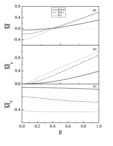
Figure 1: (a) The total magnetization density ($\bar{M}$), (b) the paramagnetization density ($\bar{M_{p}}$), and (c) the diamagnetization density ($\bar{M_{d}}$) as a function of Lande-factor $g$ at $t=0.1$. The field is chosen as $\bar{\omega}$=0.01 (solid line), 0.1 (dashed line), and 1 (dotted line).

In the following calculations we will discuss the competition between paramagnetism and diamagnetism in the 2D charged spin-1 Bose gases. Meanwhile a comparison with the 3D results Jian will also been presented.

Firstly, we look at the evolution of total magnetization density $\bar{M}$ with the Lande-factor $g$. As shown in Fig. 1(a), $\bar{M}$ is negative when $g$ is small, and changes gradually to positive after $g_{c}$. Here $g_{c}$ is the critical value of the Lande-factor $g$, where $\bar{M}$ changes its sign from negative to positive. In our model, $\bar{M}$ contains contributions come from both paramagnetism and diamagnetism. Fig. 1(b) indicates that the paramagnetization density $\bar{M}_{p}$ grows monotonously with $g$ for fixed $\bar{\omega}$. As shown in Fig. 1(c), the diamagnetization density $\bar{M}_{d}=\bar{M}-\bar{M}_{p}$ strengthens a little with increasing $g$ until saturates in the large $g$ region. Comparing to the 3D case, the diamagnetization density of 2D system is slightly dependent on $g$. While in the 3D case the diamagnetization density increases quickly with increasing $g$, especially in the small $g$ and weak magnetic field region. The curves of different magnetic field also show the stronger magnetic field is, the stronger paramagnetism and diamagnetism are at the same $g$. However the evolutionary tendency is similar qualitatively for each fixed magnetic field. According to the curves above, it is obviously that the total magnetization density is the result of the competition between paramagnetism and diamagnetism. For the case of small $g$, diamagnetism plays a major role. But the diamagnetism is covered up by the paramagnetism when $g$ exceeds $g_{c}$.

Figure 2: The critical value of Lande-factor, $g_{c}$, as a function of temperature $t$ with fixed magnetic field $\bar{\omega}$, where $\bar{\omega}=$0.1 (solid line), 1 (dashed line), 3 (dotted line), and 5 (dash-dotted line).

Figure 3: The critical value of Lande-factor, $g_{c}$, as a function of magnetic field $\bar{\omega}$ with fixed temperature $t$, where $t=$0.1 (solid line), 0.2 (dashed line), 0.5 (dotted line), and 1 (dash-dotted line).

The above results show that the shift point of Lande-factor plays a significant role in describing the competition between the paramagnetism and diamagnetism. Therefore we will focus on $g_{c}$ hereafter. $g_{c}$ can be obtained by setting $\bar{M}$=0 in equation (II). It indicates that $g_{c}$ is dependent of temperature and magnetic field. Fig. 2 plots the dependence of $g_{c}$ with temperature for fixed $\bar{\omega}$. In the low temperature limit, $g_{c}$ tends to 0.5, and $g_{c}\approx 0.35$ in the high temperature limit. In the low temperature region, the smaller $\bar{\omega}$ is, the faster $g_{c}$ declines. To further understand the effect of the magnetic field on $g_{c}$, $g_{c}$ as a function of magnetic field with fixed temperature is plotted in Fig. 3. It is shown that the $g_{c}$ limit in the weak magnetic field resembles that in the high temperature. It is interesting that $g_{c}$ reaches a uniform value when the temperature $t\longrightarrow\infty$ or the magnetic field $\bar{\omega}\longrightarrow 0$. Now we do some analytical solution to verify our numerical results.

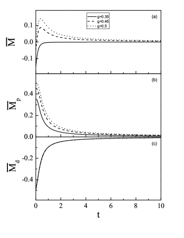
Figure 4: (a) The total magnetization density ($\bar{M}$), (b) the paramagnetization density ($\bar{M_{p}}$), and (c) the diamagnetization density ($\bar{M_{d}}$) as a function of temperature $t$ at $\bar{\omega}=1$, where Lande-factor $g$=0.35 (solid line), 0.45 (dashed line), and 0.5 (dotted line).

In the high temperature limit, Bose-Einstein statistics reduces to Maxwell-Boltzmann statistics. This makes it possible to get an exact value of $g_{c}$. Within Maxwell-Boltzmann statistics, the grand thermodynamic potential is formally expressed as

$$\Omega_{T\neq 0}=-\frac{1}{\beta}D_{L}\sum_{j,\sigma}e^{-\beta\left(\epsilon^{l}_{j}+\epsilon^{ze}_{\sigma}-\mu\right)}$$ (14)

In this case the dimensionless chemical potential $\bar{\mu}^{\prime}$ can be obtained by

$$1=\bar{\omega}\sum_{\sigma}\frac{e^{-\frac{\bar{\omega}}{t}\left(\frac{1}{2}-g\sigma-\frac{\bar{\mu}^{\prime}}{\bar{\omega}}\right)}}{1-e^{-\frac{\bar{\omega}}{t}}}$$ (15)

And the dimensionless magnetization density based on Maxwell-Boltzmann statistics can be re-expressed as

$$\bar{M}_{T\neq 0}^{B}=t\sum_{\sigma}\Bigg{\{}\frac{e^{-\frac{\bar{\omega}}{t}\left(\frac{1}{2}-g\sigma-\frac{\bar{\mu}^{\prime}}{\bar{\omega}}\right)}}{1-e^{-\frac{\bar{\omega}}{t}}}$$

$$\times\left[1+\frac{\bar{\omega}}{t}\left(g\sigma-\frac{1}{2}-\frac{e^{-\frac{\bar{\omega}}{t}}}{1-e^{-\frac{\bar{\omega}}{t}}}\right)\right]\Bigg{\}}$$ (16)

Now we substitute equation (15) into (III), then we obtain

$$\bar{M}_{T\neq 0}^{B}=\frac{1}{x}-\frac{1}{2}-\frac{1}{e^{x}-1}+g\frac{e^{gx}-e^{-gx}}{e^{gx}+e^{-gx}+1}$$ (17)

where $x={\bar{\omega}}/{t}$. As $\bar{M}_{T\neq 0}^{B}=0$, $g_{c}$ can be resolved from the analytical formula (17). In $t\longrightarrow\infty$ or $\bar{\omega}\longrightarrow 0$, $g_{c}={1}/{\sqrt{8}}\approx 0.354$. This analytical results is agreement with that presented in Fig. 2 and Fig. 3.

Figure 5: (a) The total magnetization density ($\bar{M}$), (b) the paramagnetization density ($\bar{M_{p}}$), and (c) the diamagnetization density ($\bar{M_{d}}$) as a function of magnetic field $\bar{\omega}$ at $t=0.1$, where Lande-factor $g$=0.35 (solid line), 0.45 (dashed line), and 0.5 (dotted line).

In order to manifest what affect paramagnetism and diamagnetism respectively in detail, Fig. 4 and Fig. 5 are plotted. Fig. 4 is plotted in a definite magnetic field $\bar{\omega}=1$, while Fig. 5 is given with a fixed temperature $t=0.1$. Since the two limits of $g_{c}$ are $1/2$ (low temperature or strong magnetic field) and ${1}/{\sqrt{8}}\approx 0.354$ (high temperature or weak magnetic field), the results will be shown for the three character parameters of $g$, $g=0.35$, $g=0.45$ and $g=0.5$. We explore the similarity between Fig. 4(a) and Fig. 5(a). The total magnetization density $\bar{M}$ curves of $g=0.35$ always present diamagnetism in spite of the temperature and magnetic field, while $\bar{M}$ maintain paramagnetism when $g=0.5$. But $\bar{M}$ exhibits a transition between paramagnetism and diamagnetism at $g=0.45$. This is because $g=0.45$ locates in the intermediate region between $g={1}/{\sqrt{8}}$ and $g=1/2$. It can be seen from Fig. 4(c) that diamagnetism depends mostly on the temperature in the low temperature region, regardless of the Lande-factor, until saturates at high temperature. Besides the temperature, the Lande-factor plays an important role in the paramagnetism, which is shown in Fig. 4(b). In the weak magnetic field indicated by Fig. 5(c), the magnitude of magnetic field mostly affects the diamagnetism, in spite of the Lande-factor. While in Fig. 5(b), Lande-factor dominates the paramagnetism at the strong magnetic field region.

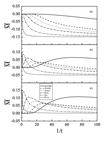
Figure 6: Plots of the total magnetization density ($\bar{M}$) as a function of $1/t$ at (a) $g$=0.35, (b) $g$=0.45 and (c) $g$=0.5, with different $\bar{\omega}$=0.0001 (solid line), 0.001 (dashed line), 0.01 (dotted line), 0.1 (dash-dotted line), 1 (dash-dot-dotted line), and 10 (short dashed line).

In order to manifest the difference in phase transition between the 2D and 3D charged spin-1 Bose system, the dependence of the total magnetization density $\bar{M}$ with $1/t$ at different magnetic fields is shown in Fig. 6. It is known that the 2D Bose gas with no external fields does not condense. In Fig. 6(a), with decreasing the magnetic field, the curve keeps smooth even in very weak magnetic field, which means no sharp bend appears in the weak field. It suggests that we can’t find a temperature which corresponding to the BEC temperature in the zero magnetic field. From Figs. 6(b) and 6(c), we can find that no intersection exists at the low temperature region in the weak magnetic field. This further proves that no condensation appears with reducing the magnetic field. The results above is different from our results of the 3D case Jian . In the 3D system, a sharp bend emerges little by little along with weakening the magnetic field. Therefore a temperature related to the BEC temperature can be predicted. This proves the key difference between the 2D and 3D charged spin-1 Bose gas.

IV Summary

In summary, we study the competition between paramagnetism and diamagnetism of a charged spin-1 Bose gas in two dimension based on the mean-field theory. In a very weak magnetic field, no condensation is predicted. It indicates the difference between the 2D and 3D system. Despite of this qualitatively distinction, some magnetic properties in 2D charged spin-1 Bose gas, such as the critical values of Lande-factor in the high temperature and low temperature limit, are similar to that of 3D case. The intriguing behavior may come from the main physics occurring in the 2D plane. Our results also show in the interplay between paramagnetism and diamagnetism, Lande-factor plays an important role in the paramagnetism, while magnetic field impacts significantly on the diamagnetism.

- (1) T. Ando, A. B. Fowler, F. Stern, Rev. Mod. Phys. 54 (1982) 437.
- (2) M. R. Schafroth, Phys. Rev. 100 (1955) 463.
- (3) J. Bardeen, L. N. Cooper, J. R. Schrieffer, Phys. Rev. 108 (1957) 1175.
- (4) R. M. May, Phys. Rev. 115 (1959) 254.
- (5) A.S. Alexandrov, Phys. Rev. Lett. 96 (2006) 147003; A.S. Alexandrov, J. Phys.: Condens. Matter 22 (2010) 426004; A.S. Alexandrov, J. Supercond. Nov. Magn. 24 (2011) 13.
- (6) M. A. Kastner, R. J. Birgeneau, G. Shirane, Y. Endoh, Rev. Mod. Phys. 70 (1998) 897.
- (7) A.S. Alexandrov, N.F. Mott, Phys. Rev. Lett. 71 (1993) 1075; R. Mincas, J. Ranninger, S. Robaszkiewicz, Rev. Mod. Phys. 62 (1992) 113.
- (8) D. F. Hines, N. E. Frankel, Phys. Rev. B 20 (1979) 972.
- (9) D. C. Bardos, D. F. Hines, N. E. Frankel, Phys. Rev. B 49 (1994) 4082.
- (10) B. Davoudi, E. Strepparola, B. Tanatar, M. P. Tosi, Phys. Rev. B 63 (2001) 104505.
- (11) J. Daicic, N. E. Frankel, Phys. Rev. B 55 (1997) 2760.
- (12) B. P. van Zyl, D. A. W. Hutchinson, Phys. Rev. B 69 (2004) 024520.
- (13) J. Daicic, N. E. Frankel, V. Kowalenko, Phys. Rev. Lett. 71 (1993) 1779; J. Daicic , N. E. Frankel, R. M. Gailis, V. Kowalenko, Phys. Rep. 237 (1994) 63; J. Daicic, N. E. Frankel, Phys. Rev. D 53 (1996) 5745.
- (14) D. J. Toms, Phys. Rev. B 50 (1994) 3120; D. J. Toms, Phys. Rev. D 51 (1995) 1886; G. B. Standen, D. J. Toms, Phys. Rev. E 60 (1999) 5275.
- (15) X. L. Jian, J. H. Qin, Q. Gu, J. Phys.: Condens. Matter 23 (2011) 026003.
- (16) J. H. Qin, X. L. Jian, Q. Gu, J. Phys.: Condens. Matter 24 (2012) 366007.
- (17) R. M. May, J. Math. Phys. 6 (1965) 1462.