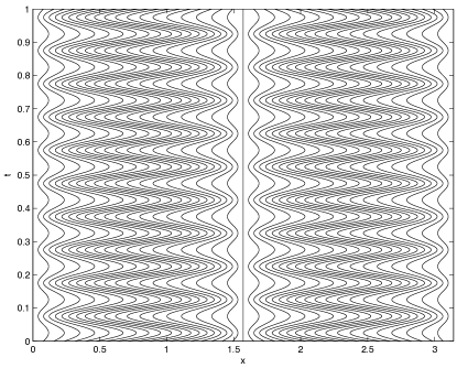
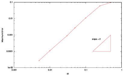
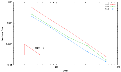
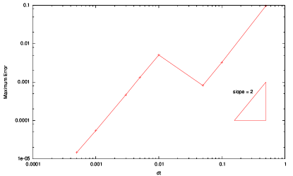
Unconditionally stable high-order time integration for moving mesh finite difference solution of linear convection-diffusion equations

Weizhang Huang Department of Mathematics, the University of Kansas, Lawrence, KS 66045, U.S.A. (huang@math.ku.edu). This work was supported in part by the NSF under Grants DMS-0712935 and DMS-1115118.
Abstract

This paper is concerned with moving mesh finite difference solution of partial differential equations. It is known that mesh movement introduces an extra convection term and its numerical treatment has a significant impact on the stability of numerical schemes. Moreover, many implicit second and higher order schemes, such as the Crank-Nicolson scheme, will loss their unconditional stability. A strategy is presented for developing temporally high order, unconditionally stable finite difference schemes for solving linear convection-diffusion equations using moving meshes. Numerical results are given to demonstrate the theoretical findings.

AMS 2010 Mathematics Subject Classification. 65M06, 65M12, 65L20

Key Words. Moving mesh, high order method, time integration, stability, finite difference.

Abbreviated title. Unconditionally stable high order time integration on moving meshes.

1 Introduction

In the last two decades, moving mesh methods have attracted considerable attention from scientists and engineers and been successfully applied to a variety of problems; e.g., see [8, 21] and references therein. A common feature of those methods is that they employ a time varying mesh to follow the motion of the physical boundary and/or certain solution properties. Generally speaking, partial differential equations (PDEs) can be discretized directly on a moving mesh using finite element and finite volume methods. When a finite difference method is desired, it is common practice to transform PDEs to a reference domain and discretize them on a fixed mesh defined thereon. The interested reader is referred to [21] for more detailed discussion on the discretization of PDEs on moving meshes. It should be emphasized that, despite what discretization method is used, the movement of the mesh inevitably introduces an extra convection term into PDEs, whose numerical treatment often has a significant impact on the stability and convergence of moving mesh methods. The term also makes the analysis of stability and convergence much more difficult for moving mesh methods even when linear PDEs are involved.

While a number of convergence results have been developed for the numerical solution of two-point boundary value problems using equidistributing meshes (a type of moving meshes) (e.g., see [4, 5, 6, 9, 16, 20, 23, 25, 27, 28]), theoretical studies of moving mesh methods for time dependent PDEs are far from complete. For example, for linear convection-diffusion problems Dupont [11], Bank and Santos [3], Dupont and Liu [12], and Liu et al. [24] establish symmetric error estimates for various finite element methods (FEM), including semi-discrete FEM, semi-discrete mixed FEM, FEM-implicit Euler, and space-time FEM. These results essentially require the conditions (or their discrete counterparts)

|𝒙˙(𝒙,t)𝒃(𝒙,t)|C1,𝒙Ω,t>0formulae-sequence˙𝒙𝒙𝑡𝒃𝒙𝑡subscript𝐶1formulae-sequencefor-all𝒙Ω𝑡0\displaystyle|\dot{\mbox{\boldmath$x$}}(\mbox{\boldmath$x$},t)-\mbox{\boldmath$b$}(\mbox{\boldmath$x$},t)|\leq C_{1},\quad\forall\mbox{\boldmath$x$}\in\Omega,\;t>0 (1)
|𝒙˙(𝒙,t)|C2,𝒙Ω,t>0formulae-sequence˙𝒙𝒙𝑡subscript𝐶2formulae-sequencefor-all𝒙Ω𝑡0\displaystyle|\nabla\cdot\dot{\mbox{\boldmath$x$}}(\mbox{\boldmath$x$},t)|\leq C_{2},\quad\forall\mbox{\boldmath$x$}\in\Omega,\;t>0 (2)

where C1subscript𝐶1C_{1} and C2subscript𝐶2C_{2} are positive constants, ΩΩ\Omega is the physical domain, 𝒙˙˙𝒙\dot{\mbox{\boldmath$x$}} is the mesh speed, and 𝒃𝒃b is the coefficient of the convection term (see (5) below). Condition (1) requires that the mesh move not too fast with reference to 𝒃𝒃b. To see the geometric meaning of (2), we view the moving mesh as the image of a computational mesh under a coordinate transformation 𝒙=𝒙(𝝃,t)𝒙𝒙𝝃𝑡\mbox{\boldmath$x$}=\mbox{\boldmath$x$}(\mbox{\boldmath$\xi$},t): ΩcΩsubscriptΩ𝑐Ω\Omega_{c}\to\Omega, where ΩcsubscriptΩ𝑐\Omega_{c} is the computational domain. Denote the Jacobian of the coordinate transformation by J𝐽J, i.e., J=det(𝒙/𝝃)𝐽det𝒙𝝃J=\mbox{det}(\partial\mbox{\boldmath$x$}/\partial\mbox{\boldmath$\xi$}). It is known [21] that

1JJ˙=𝒙˙.1𝐽˙𝐽˙𝒙\frac{1}{J}\dot{J}=\nabla\cdot\dot{\mbox{\boldmath$x$}}.

Then (2) reduces to

|J˙|C2|J|.˙𝐽subscript𝐶2𝐽|\dot{J}|\leq C_{2}|J|. (3)

Since J𝐽J represents the volume of mesh elements, (3), or equivalently (2), requires that the relative change of the volume of mesh elements be in a constant order.

Formaggia and Nobile [14, 15] and Boffi and Gastaldi [7] study the relation between stability and satisfaction of the geometric conservation law (GCL) [29] in the Arbitrary-Langragian-Eulerian formulation [19] with finite element spatial discretization. They show that satisfying GCL is neither a necessary nor a sufficient condition for the stability of a scheme although it often helps improve accuracy and enhance stability. In particular, Boffi and Gastaldi show that the FEM-implicit Euler scheme is only conditionally stable. Formaggia and Nobile [14, 15] present several modifications of the implicit Euler, Crank-Nicolson, and BDF2 (two step backward differentiation formula [10, 17]) schemes, which can be made to satisfy GCL. They show that the FEM-modified implicit Euler scheme is unconditionally stable whereas the FEM-modified Crank-Nicolson and FEM-BDF(2) schemes are only conditionally stable with the maximum allowable time step depending on 𝒙˙˙𝒙\nabla\cdot\dot{\mbox{\boldmath$x$}}.

Ferreira [13] studies a finite difference (FDM)-implicit Euler scheme applied to the nonconservative form of transformed linear convection-diffusion equations and shows that the scheme is stable and convergent under discrete analogs of conditions (1) and (3). Mackenzie and Mekwi [26] consider an FDM-θ𝜃\theta scheme for the conservative form of transformed linear convection-diffusion equations. They show that the FDM-implict Euler scheme is unconditionally stable in an energy norm but the Crank-Nicolson scheme is only conditionally stable. They also show that the FDM-θ𝜃\theta scheme can be made to be unconditionally stable and of second order in time (and in space) when θ𝜃\theta is properly chosen depending on the mesh. Although this variable θ𝜃\theta scheme is unconventional, there are no other moving mesh methods that are known to be of second or higher order in time and unconditionally stable. More recently, Huang and Schaeffer [22] show that several FDM-θ𝜃\theta moving mesh schemes for one dimensional convection-diffusion problems are stable in Lsuperscript𝐿L^{\infty} norm under the conventional CFL condition and a mesh speed related condition which can be roughly expressed as

|x˙b|C3h,˙𝑥𝑏subscript𝐶3|\dot{x}-b|\leq\frac{C_{3}}{h}, (4)

where C3subscript𝐶3C_{3} is a constant and hh is the maximum spacing of the mesh. Notice that this condition is weaker than (1).

It is well known that high-order methods are practically important in enhancing the computational accuracy and efficiency. It is also important in theory to know if unconditionally stable high-order methods exist in the moving mesh context. The objective of this paper is to develop unconditionally stable, high-order (in time) moving finite difference schemes for the solution of the initial-boundary value problem (IBVP) of a general linear convection-diffusion equation,

{ut+(u𝒃)+cu=(au)+f,𝒙Ω,t(0,T]u(𝒙,t)=g(𝒙,t),𝒙Ωu(𝒙,0)=u0(𝒙),𝒙Ωcasesformulae-sequence𝑢𝑡𝑢𝒃𝑐𝑢𝑎𝑢𝑓formulae-sequencefor-all𝒙Ω𝑡0𝑇otherwiseformulae-sequence𝑢𝒙𝑡𝑔𝒙𝑡for-all𝒙Ωotherwiseformulae-sequence𝑢𝒙0superscript𝑢0𝒙for-all𝒙Ωotherwise\begin{cases}\frac{\partial u}{\partial t}+\nabla\cdot(u\mbox{\boldmath$b$})+cu=\nabla\cdot(a\nabla u)+f,\quad\forall\mbox{\boldmath$x$}\in\Omega,\;t\in(0,T]\\ u(\mbox{\boldmath$x$},t)=g(\mbox{\boldmath$x$},t),\quad\forall\mbox{\boldmath$x$}\in\partial\Omega\\ u(\mbox{\boldmath$x$},0)=u^{0}(\mbox{\boldmath$x$}),\quad\forall\mbox{\boldmath$x$}\in\Omega\end{cases} (5)

where ΩdΩsuperscript𝑑\Omega\subset\mathbb{R}^{d} (d=1,2𝑑12d=1,2) is the physical domain with probably moving or deforming boundary and a=a(𝒙,t)𝑎𝑎𝒙𝑡a=a(\mbox{\boldmath$x$},t), 𝒃=𝒃(𝒙,t)𝒃𝒃𝒙𝑡\mbox{\boldmath$b$}=\mbox{\boldmath$b$}(\mbox{\boldmath$x$},t), c=c(𝒙,t)𝑐𝑐𝒙𝑡c=c(\mbox{\boldmath$x$},t), f=f(𝒙,t)𝑓𝑓𝒙𝑡f=f(\mbox{\boldmath$x$},t), g=g(𝒙,t)𝑔𝑔𝒙𝑡g=g(\mbox{\boldmath$x$},t), and u0(𝒙)superscript𝑢0𝒙u^{0}(\mbox{\boldmath$x$}) are given, sufficiently smooth functions. For the posedness of IBVP, we assume that the coefficients satisfy

0<a¯a(𝒙,t)a¯<,𝒙Ω,t(0,T]formulae-sequence0¯𝑎𝑎𝒙𝑡¯𝑎formulae-sequencefor-all𝒙Ω𝑡0𝑇\displaystyle 0<\underline{a}\leq a(\mbox{\boldmath$x$},t)\leq\overline{a}<\infty,\quad\forall\mbox{\boldmath$x$}\in\Omega,\;t\in(0,T] (6)
c(𝒙,t)+12𝒃(𝒙,t)0,𝒙Ω,t(0,T]formulae-sequence𝑐𝒙𝑡12𝒃𝒙𝑡0formulae-sequencefor-all𝒙Ω𝑡0𝑇\displaystyle c(\mbox{\boldmath$x$},t)+\frac{1}{2}\nabla\cdot\mbox{\boldmath$b$}(\mbox{\boldmath$x$},t)\geq 0,\quad\forall\mbox{\boldmath$x$}\in\Omega,\;t\in(0,T] (7)

where a¯¯𝑎\underline{a} and a¯¯𝑎\overline{a} are two positive constants. We note that for stability analysis, we only need to consider the homogeneous system, i.e., the IBVP with f0𝑓0f\equiv 0 and g0𝑔0g\equiv 0. In this situation, it is easy to show that the solution satisfies the stability inequality

ddtΩu2𝑑𝒙0.𝑑𝑑𝑡subscriptΩsuperscript𝑢2differential-d𝒙0\frac{d}{dt}\int_{\Omega}u^{2}d\mbox{\boldmath$x$}\leq 0. (8)

The key to our development is the preservation of stability inequality (8). We use the method of lines approach and first discretize the PDE in space in such a way that the resulting system of ordinary differential equations (ODEs) satisfies a semi-discrete stability inequality. Then high-order schemes satisfying a fully discrete version of (8) are constructed for integrating the ODE system. The resulting schemes are stable in the energy norm corresponding to the fully discrete stability inequality.

An outline of this paper is given as follows. In §2, high-order unconditionally stable schemes for ODE systems satisfying a stability inequality are developed. Strategies for spatially discretizing IBVP (5) into such an ODE system in one and two dimensions are explored in §3 and §4. Numerical examples obtained with the developed schemes are presented in §5. Finally, §6 contains conclusions and comments.

2 High-order unconditionally stable schemes for nonautonomous ODE systems

In this section we present an approach of constructing unconditionally stable schemes for the initial value problem of a nonautonomous ODE system

{M(t)d𝒖dt=A(t)𝒖+𝒇(t),𝒖(0)=𝒖0cases𝑀𝑡𝑑𝒖𝑑𝑡𝐴𝑡𝒖𝒇𝑡otherwise𝒖0superscript𝒖0otherwise\begin{cases}M(t)\frac{d\mbox{\boldmath$u$}}{dt}=A(t)\mbox{\boldmath$u$}+\mbox{\boldmath$f$}(t),\\ \mbox{\boldmath$u$}(0)=\mbox{\boldmath$u$}^{0}\end{cases} (9)

where M(t)𝑀𝑡M(t) and A(t)𝐴𝑡A(t) are l×l𝑙𝑙l\times l matrices (for some positive integer l𝑙l) and 𝒇(t)𝒇𝑡\mbox{\boldmath$f$}(t) is a given vector-valued function. We assume that M(t)𝑀𝑡M(t) is symmetric and positive definite and A(t)+M(t)dMdt(t)𝐴𝑡𝑀𝑡𝑑𝑀𝑑𝑡𝑡A(t)+\sqrt{M}(t)\frac{d\sqrt{M}}{dt}(t) is negative semi-definite, i.e.,

𝒛T(A(t)+M(t)dMdt(t))𝒛0,𝒛l,t>0formulae-sequencesuperscript𝒛𝑇𝐴𝑡𝑀𝑡𝑑𝑀𝑑𝑡𝑡𝒛0formulae-sequencefor-all𝒛superscript𝑙for-all𝑡0\mbox{\boldmath$z$}^{T}\left(A(t)+\sqrt{M}(t)\frac{d\sqrt{M}}{dt}(t)\right)\mbox{\boldmath$z$}\leq 0,\quad\forall\mbox{\boldmath$z$}\in\mathbb{R}^{l},\quad\forall t>0 (10)

where M𝑀\sqrt{M} denotes the square root of M𝑀M. As will be seen in §3 and §4, such systems arise from finite difference discretization of IBVP (5) on moving meshes, with M(t)𝑀𝑡M(t) and A(t)𝐴𝑡A(t) being the mass and stiffness matrices, respectively.

The idea of the approach is simple. Indeed, we rewrite (9) into

ddt(M𝒖)=(M)1(A+MdMdt)𝒖+(M)1𝒇,𝑑𝑑𝑡𝑀𝒖superscript𝑀1𝐴𝑀𝑑𝑀𝑑𝑡𝒖superscript𝑀1𝒇\frac{d}{dt}\left(\sqrt{M}\mbox{\boldmath$u$}\right)=(\sqrt{M})^{-1}\left(A+\sqrt{M}\frac{d\sqrt{M}}{dt}\right)\mbox{\boldmath$u$}+(\sqrt{M})^{-1}\mbox{\boldmath$f$}, (11)

which can further be written as

d𝒗dt=B(t)𝒗+(M(t))1𝒇(t),𝑑𝒗𝑑𝑡𝐵𝑡𝒗superscript𝑀𝑡1𝒇𝑡\frac{d\mbox{\boldmath$v$}}{dt}=B(t)\mbox{\boldmath$v$}+(\sqrt{M}(t))^{-1}\mbox{\boldmath$f$}(t), (12)

where

𝒗(t)=M(t)𝒖(t),𝒗𝑡𝑀𝑡𝒖𝑡\displaystyle\mbox{\boldmath$v$}(t)=\sqrt{M}(t)\mbox{\boldmath$u$}(t), (13)
B(t)=(M)1(A+MdMdt)(M)1.𝐵𝑡superscript𝑀1𝐴𝑀𝑑𝑀𝑑𝑡superscript𝑀1\displaystyle B(t)=(\sqrt{M})^{-1}\left(A+\sqrt{M}\frac{d\sqrt{M}}{dt}\right)(\sqrt{M})^{-1}. (14)

Then, unconditionally stable schemes can be obtained by applying conventional implicit schemes to (12). The initial condition for the new variable is

𝒗(0)=𝒗0M(0)𝒖0.𝒗0superscript𝒗0𝑀0superscript𝒖0\mbox{\boldmath$v$}(0)=\mbox{\boldmath$v$}^{0}\equiv\sqrt{M}(0)\mbox{\boldmath$u$}^{0}. (15)

Moreover, assumption (10) implies that B(t)𝐵𝑡B(t) is negative semi-definite for any t>0𝑡0t>0.

In the following, we illustrate the idea with three schemes. To this end, we assume that a partition is given for [0,T]0𝑇[0,T],

t0=0<t1<<tN=T.subscript𝑡00subscript𝑡1subscript𝑡𝑁𝑇t_{0}=0<t_{1}<\cdots<t_{N}=T.

We denote Δtn=tn+1tnΔsubscript𝑡𝑛subscript𝑡𝑛1subscript𝑡𝑛\Delta t_{n}=t_{n+1}-t_{n}.

We first apply the backward Euler discretization to (12). It gives

𝒗n+1𝒗nΔtn=B(tn+1)𝒗n+1+(M(tn+1))1𝒇(tn+1).superscript𝒗𝑛1superscript𝒗𝑛Δsubscript𝑡𝑛𝐵subscript𝑡𝑛1superscript𝒗𝑛1superscript𝑀subscript𝑡𝑛11𝒇subscript𝑡𝑛1\frac{\mbox{\boldmath$v$}^{n+1}-\mbox{\boldmath$v$}^{n}}{\Delta t_{n}}=B(t_{n+1})\;\mbox{\boldmath$v$}^{n+1}+(\sqrt{M}(t_{n+1}))^{-1}\mbox{\boldmath$f$}(t_{n+1}). (16)

Since B𝐵B is negative semi-definite, for the homogeneous situation (with 𝒇=0𝒇0\mbox{\boldmath$f$}=0) we can readily show that (16) satisfies

(𝒗n+1)T𝒗n+1(𝒗n)T𝒗n,superscriptsuperscript𝒗𝑛1𝑇superscript𝒗𝑛1superscriptsuperscript𝒗𝑛𝑇superscript𝒗𝑛(\mbox{\boldmath$v$}^{n+1})^{T}\mbox{\boldmath$v$}^{n+1}\leq(\mbox{\boldmath$v$}^{n})^{T}\mbox{\boldmath$v$}^{n}, (17)

which can be written in terms of the original variable 𝒖𝒖u as

(𝒖n+1)TM(tn+1)𝒖n+1(𝒖n)TM(tn)𝒖n.superscriptsuperscript𝒖𝑛1𝑇𝑀subscript𝑡𝑛1superscript𝒖𝑛1superscriptsuperscript𝒖𝑛𝑇𝑀subscript𝑡𝑛superscript𝒖𝑛(\mbox{\boldmath$u$}^{n+1})^{T}\sqrt{M}(t_{n+1})\mbox{\boldmath$u$}^{n+1}\leq(\mbox{\boldmath$u$}^{n})^{T}\sqrt{M}(t_{n})\mbox{\boldmath$u$}^{n}. (18)

Inequality (18) is a discrete analog to (8). It implies that the backward Euler scheme (16), which is of first order, is unconditionally stable.

A second order unconditionally stable scheme can be obtained by applying the midpoint discretization to (12). Indeed, we have

𝒗n+1𝒗nΔtn=B(tn+tn+12)𝒗n+1+𝒗n2+(M(tn+tn+12))1𝒇(tn+tn+12).superscript𝒗𝑛1superscript𝒗𝑛Δsubscript𝑡𝑛𝐵subscript𝑡𝑛subscript𝑡𝑛12superscript𝒗𝑛1superscript𝒗𝑛2superscript𝑀subscript𝑡𝑛subscript𝑡𝑛121𝒇subscript𝑡𝑛subscript𝑡𝑛12\frac{\mbox{\boldmath$v$}^{n+1}-\mbox{\boldmath$v$}^{n}}{\Delta t_{n}}=B\left(\frac{t_{n}+t_{n+1}}{2}\right)\frac{\mbox{\boldmath$v$}^{n+1}+\mbox{\boldmath$v$}^{n}}{2}+\left(\sqrt{M}\left(\frac{t_{n}+t_{n+1}}{2}\right)\right)^{-1}\mbox{\boldmath$f$}\left(\frac{t_{n}+t_{n+1}}{2}\right). (19)

It is easy to show that the solution of (19) (with 𝒇=0𝒇0\mbox{\boldmath$f$}=0) satisfies stability inequality (17).

Higher order unconditionally stable schemes can be obtained by applying collocation schemes to (12). To explain this, we consider the m𝑚m Gauss-Legendre points in (0,1)01(0,1), ρ1subscript𝜌1\rho_{1}, …, ρmsubscript𝜌𝑚\rho_{m}, and denote the collocation points by

tn,j=tn+ρjΔtn,j=1,,m.formulae-sequencesubscript𝑡𝑛𝑗subscript𝑡𝑛subscript𝜌𝑗Δsubscript𝑡𝑛𝑗1𝑚t_{n,j}=t_{n}+\rho_{j}\Delta t_{n},\quad j=1,...,m. (20)

Applying the m𝑚m-point collocation scheme (e.g., see [1, 2]) to (12), we get, for n=0,,N1𝑛0𝑁1n=0,...,N-1,

d𝒗hdt(tn,j)=B(tn,j)𝒗h(tn,j)+(M(tn,j))1𝒇(tn,j),j=1,,mformulae-sequence𝑑subscript𝒗𝑑𝑡subscript𝑡𝑛𝑗𝐵subscript𝑡𝑛𝑗subscript𝒗subscript𝑡𝑛𝑗superscript𝑀subscript𝑡𝑛𝑗1𝒇subscript𝑡𝑛𝑗𝑗1𝑚\frac{d\mbox{\boldmath$v$}_{h}}{dt}(t_{n,j})=B(t_{n,j})\mbox{\boldmath$v$}_{h}(t_{n,j})+(\sqrt{M}(t_{n,j}))^{-1}\mbox{\boldmath$f$}(t_{n,j}),\quad j=1,...,m (21)

where 𝒗h(t)subscript𝒗𝑡\mbox{\boldmath$v$}_{h}(t), an approximation to the exact solution 𝒗(t)𝒗𝑡\mbox{\boldmath$v$}(t), is continuous on [0,T]0𝑇[0,T] and a polynomial of degree m𝑚m on each subinterval [tn,tn+1]subscript𝑡𝑛subscript𝑡𝑛1[t_{n},t_{n+1}].

We can rewrite (21) into a more explicit form. Let ρ~1subscript~𝜌1\tilde{\rho}_{1}, …, ρ~m1subscript~𝜌𝑚1\tilde{\rho}_{m-1} be the (m1)𝑚1(m-1) Gauss-Legendre points in (0,1)01(0,1) and denote ρ~0=0subscript~𝜌00\tilde{\rho}_{0}=0 and ρ~m=1subscript~𝜌𝑚1\tilde{\rho}_{m}=1. Define

t~n,j=tn+ρ~jΔtn,j=0,,m.formulae-sequencesubscript~𝑡𝑛𝑗subscript𝑡𝑛subscript~𝜌𝑗Δsubscript𝑡𝑛𝑗0𝑚\tilde{t}_{n,j}=t_{n}+\tilde{\rho}_{j}\Delta t_{n},\quad j=0,...,m. (22)

(We may also take ρ~0,,ρ~msubscript~𝜌0subscript~𝜌𝑚\tilde{\rho}_{0},...,\tilde{\rho}_{m} as the (m+1)𝑚1(m+1) Gauss-Lobatto Legendre points on [0,1]01[0,1].) Then, 𝒗hsubscript𝒗\mbox{\boldmath$v$}_{h} can be expressed as

𝒗h(t)=k=0m𝒗~n,k~k(ttnΔtn),t[tn,tn+1],n=0,,N1formulae-sequencesubscript𝒗𝑡superscriptsubscript𝑘0𝑚subscript~𝒗𝑛𝑘subscript~𝑘𝑡subscript𝑡𝑛Δsubscript𝑡𝑛formulae-sequencefor-all𝑡subscript𝑡𝑛subscript𝑡𝑛1𝑛0𝑁1\mbox{\boldmath$v$}_{h}(t)=\sum_{k=0}^{m}\tilde{\mbox{\boldmath$v$}}_{n,k}\tilde{\ell}_{k}\left(\frac{t-t_{n}}{\Delta t_{n}}\right),\quad\forall t\in[t_{n},t_{n+1}],\;n=0,...,N-1 (23)

where 𝒗~n,k𝒗(t~n,k)subscript~𝒗𝑛𝑘𝒗subscript~𝑡𝑛𝑘\tilde{\mbox{\boldmath$v$}}_{n,k}\approx\mbox{\boldmath$v$}(\tilde{t}_{n,k}) (k=0,,m𝑘0𝑚k=0,...,m) are the unknown variables and ~ksubscript~𝑘\tilde{\ell}_{k}’s are the Lagrange polynomials associated with nodes ρ~0subscript~𝜌0\tilde{\rho}_{0}, …, ρ~msubscript~𝜌𝑚\tilde{\rho}_{m}, i.e.,

~k(ρ)=i=0ikmρρ~iρ~kρ~i.subscript~𝑘𝜌superscriptsubscriptproductFRACOP𝑖0𝑖𝑘𝑚𝜌subscript~𝜌𝑖subscript~𝜌𝑘subscript~𝜌𝑖\tilde{\ell}_{k}(\rho)=\prod\limits_{i=0\atop i\neq k}^{m}\frac{\rho-\tilde{\rho}_{i}}{\tilde{\rho}_{k}-\tilde{\rho}_{i}}.

Inserting (23) into (21), we have

1Δtnk=0m𝒗~n,k~k(ρj)=B(tn,j)k=0m𝒗~n,k~k(ρj)+(M(tn,j))1𝒇(tn,j),j=1,,mformulae-sequence1Δsubscript𝑡𝑛superscriptsubscript𝑘0𝑚subscript~𝒗𝑛𝑘superscriptsubscript~𝑘subscript𝜌𝑗𝐵subscript𝑡𝑛𝑗superscriptsubscript𝑘0𝑚subscript~𝒗𝑛𝑘subscript~𝑘subscript𝜌𝑗superscript𝑀subscript𝑡𝑛𝑗1𝒇subscript𝑡𝑛𝑗𝑗1𝑚\frac{1}{\Delta t_{n}}\sum\limits_{k=0}^{m}\tilde{\mbox{\boldmath$v$}}_{n,k}\tilde{\ell}_{k}^{\;{}^{\prime}}\left(\rho_{j}\right)=B(t_{n,j})\sum\limits_{k=0}^{m}\tilde{\mbox{\boldmath$v$}}_{n,k}\tilde{\ell}_{k}\left(\rho_{j}\right)+(\sqrt{M}(t_{n,j}))^{-1}\mbox{\boldmath$f$}(t_{n,j}),\quad j=1,...,m (24)

This equation, together with the initial condition

𝒗~n,0=𝒗~n1,m,subscript~𝒗𝑛0subscript~𝒗𝑛1𝑚\tilde{\mbox{\boldmath$v$}}_{n,0}=\tilde{\mbox{\boldmath$v$}}_{n-1,m}, (25)

forms a system of ODEs for unknowns 𝒗~n,ksubscript~𝒗𝑛𝑘\tilde{\mbox{\boldmath$v$}}_{n,k}, k=0,,m𝑘0𝑚k=0,...,m.

Once 𝒗~n,msubscript~𝒗𝑛𝑚\tilde{\mbox{\boldmath$v$}}_{n,m} has been obtained, we can compute the original variable 𝒖𝒖u at t=tn+1𝑡subscript𝑡𝑛1t=t_{n+1} by

𝒖n+1=(M)1(tn+1)𝒗~n,m,n=0,,N1.formulae-sequencesuperscript𝒖𝑛1superscript𝑀1subscript𝑡𝑛1subscript~𝒗𝑛𝑚𝑛0𝑁1\mbox{\boldmath$u$}^{n+1}=(\sqrt{M})^{-1}(t_{n+1})\;\tilde{\mbox{\boldmath$v$}}_{n,m},\quad n=0,...,N-1. (26)

Moreover, it is known (e.g., see [1, 2]) that the convergence order of the m𝑚m-point collocation scheme (21) is 2m2𝑚2m. (It is easy to verify that scheme (21) reduces to the midpoint scheme (19) when m=1𝑚1m=1.)

In the following we show that scheme (21) (with 𝒇=0𝒇0\mbox{\boldmath$f$}=0) satisfies (17). To this end, we denote 𝒗n+1=𝒗~n,msuperscript𝒗𝑛1subscript~𝒗𝑛𝑚\mbox{\boldmath$v$}^{n+1}=\tilde{\mbox{\boldmath$v$}}_{n,m} for n=0,,N1𝑛0𝑁1n=0,...,N-1. Obviously, 𝒗n+1=𝒗h(tn+1)superscript𝒗𝑛1subscript𝒗subscript𝑡𝑛1\mbox{\boldmath$v$}^{n+1}=\mbox{\boldmath$v$}_{h}(t_{n+1}). Let ω1,,ωmsubscript𝜔1subscript𝜔𝑚\omega_{1},\,\cdots,\,\omega_{m} be the weights for the Gaussian quadrature rule associated with the points ρ1,,ρmsubscript𝜌1subscript𝜌𝑚\rho_{1},\,\cdots,\,\rho_{m}, viz.,

01f(ρ)𝑑ρj=1mωjf(ρj).superscriptsubscript01𝑓𝜌differential-d𝜌superscriptsubscript𝑗1𝑚subscript𝜔𝑗𝑓subscript𝜌𝑗\int_{0}^{1}f(\rho)d\rho\approx\sum_{j=1}^{m}\omega_{j}f(\rho_{j}).

It is known that ωjsubscript𝜔𝑗\omega_{j}’s are positive and the quadrature rule is exact for all polynomials of degree up to (2m1)2𝑚1(2m-1). Multiplying (21) with Δtnωj𝒗h(tn,j)TΔsubscript𝑡𝑛subscript𝜔𝑗subscript𝒗superscriptsubscript𝑡𝑛𝑗𝑇\Delta t_{n}\omega_{j}\mbox{\boldmath$v$}_{h}(t_{n,j})^{T} and summing the result over j𝑗j, we have

Δtnj=1mωj𝒗h(tn,j)Td𝒗hdt(tn,j)=Δtnj=1mωj𝒗h(tn,j)TB(tn,j)𝒗h(tn,j).Δsubscript𝑡𝑛superscriptsubscript𝑗1𝑚subscript𝜔𝑗subscript𝒗superscriptsubscript𝑡𝑛𝑗𝑇𝑑subscript𝒗𝑑𝑡subscript𝑡𝑛𝑗Δsubscript𝑡𝑛superscriptsubscript𝑗1𝑚subscript𝜔𝑗subscript𝒗superscriptsubscript𝑡𝑛𝑗𝑇𝐵subscript𝑡𝑛𝑗subscript𝒗subscript𝑡𝑛𝑗\Delta t_{n}\sum_{j=1}^{m}\omega_{j}\mbox{\boldmath$v$}_{h}(t_{n,j})^{T}\frac{d\mbox{\boldmath$v$}_{h}}{dt}(t_{n,j})=\Delta t_{n}\sum_{j=1}^{m}\omega_{j}\mbox{\boldmath$v$}_{h}(t_{n,j})^{T}B(t_{n,j})\mbox{\boldmath$v$}_{h}(t_{n,j}).

The negative semi-definiteness of B𝐵B implies that the right-hand side is nonpositive. Moreover, 𝒗hTd𝒗hdtsuperscriptsubscript𝒗𝑇𝑑subscript𝒗𝑑𝑡\mbox{\boldmath$v$}_{h}^{T}\frac{d\mbox{\boldmath$v$}_{h}}{dt} is a polynomial of degree at most (2m1)2𝑚1(2m-1) and the sum on the left-hand side is equal to the integral of 𝒗hTd𝒗hdtsuperscriptsubscript𝒗𝑇𝑑subscript𝒗𝑑𝑡\mbox{\boldmath$v$}_{h}^{T}\frac{d\mbox{\boldmath$v$}_{h}}{dt} over [tn,tn+1]subscript𝑡𝑛subscript𝑡𝑛1[t_{n},t_{n+1}]. Thus, we have

tntn+1𝒗hTd𝒗hdt𝑑t0.superscriptsubscriptsubscript𝑡𝑛subscript𝑡𝑛1superscriptsubscript𝒗𝑇𝑑subscript𝒗𝑑𝑡differential-d𝑡0\int_{t_{n}}^{t_{n+1}}\mbox{\boldmath$v$}_{h}^{T}\frac{d\mbox{\boldmath$v$}_{h}}{dt}dt\leq 0.

This, combined with the fact that

tntn+1𝒗hTd𝒗hdt𝑑t=12tntn+1ddt(𝒗hT𝒗h)𝑑t=12((𝒗n+1)T𝒗n+1(𝒗n)T𝒗n),superscriptsubscriptsubscript𝑡𝑛subscript𝑡𝑛1superscriptsubscript𝒗𝑇𝑑subscript𝒗𝑑𝑡differential-d𝑡12superscriptsubscriptsubscript𝑡𝑛subscript𝑡𝑛1𝑑𝑑𝑡superscriptsubscript𝒗𝑇subscript𝒗differential-d𝑡12superscriptsuperscript𝒗𝑛1𝑇superscript𝒗𝑛1superscriptsuperscript𝒗𝑛𝑇superscript𝒗𝑛\int_{t_{n}}^{t_{n+1}}\mbox{\boldmath$v$}_{h}^{T}\frac{d\mbox{\boldmath$v$}_{h}}{dt}dt=\frac{1}{2}\int_{t_{n}}^{t_{n+1}}\frac{d}{dt}\left(\mbox{\boldmath$v$}_{h}^{T}\mbox{\boldmath$v$}_{h}\right)dt=\frac{1}{2}((\mbox{\boldmath$v$}^{n+1})^{T}\mbox{\boldmath$v$}^{n+1}-(\mbox{\boldmath$v$}^{n})^{T}\mbox{\boldmath$v$}^{n}),

leads to (17).

It is remarked that scheme (21) is expressed in the new variable 𝒗𝒗v. It can be reformulated in terms of the original variable 𝒖𝒖u using the relation (13). Moreover, scheme (21) involves M𝑀\sqrt{M} and its inverse whose computation can be expensive in general. In our current situation with finite difference discretization for PDEs, however, the mass matrix M𝑀M is diagonal and its square root and the inverse can be computed easily (see the next two sections) and thus the involvement of M𝑀\sqrt{M} and its inverse has very mild effects on the computational efficiency. The argument also goes for finite volume methods or finite element methods with lumped mass matrix.

3 1D convection-diffusion equations

In this and next sections, we study the finite difference discretization of IBVP (5). Our goal is to obtain schemes that satisfy the property (10) and thus unconditionally stable integration schemes can be developed. We consider one dimensional convection-diffusion equations in this section and two dimensional ones in the next section.

In one dimension, IBVP (5) becomes

{ut+(bu)x+cu=(aux)x+f,x(xl(t),xr(t)),0<tTu(xl(t),t)=g(xl(t),t),u(xr(t),t)=g(xr(t),t),u(x,t)=u0(x).casesformulae-sequencesubscript𝑢𝑡subscript𝑏𝑢𝑥𝑐𝑢subscript𝑎subscript𝑢𝑥𝑥𝑓formulae-sequencefor-all𝑥subscript𝑥𝑙𝑡subscript𝑥𝑟𝑡0𝑡𝑇otherwiseformulae-sequence𝑢subscript𝑥𝑙𝑡𝑡𝑔subscript𝑥𝑙𝑡𝑡𝑢subscript𝑥𝑟𝑡𝑡𝑔subscript𝑥𝑟𝑡𝑡otherwise𝑢𝑥𝑡superscript𝑢0𝑥otherwise\begin{cases}u_{t}+(bu)_{x}+cu=(au_{x})_{x}+f,\qquad\forall x\in(x_{l}(t),x_{r}(t)),\quad 0<t\leq T\\ u(x_{l}(t),t)=g(x_{l}(t),t),\quad u(x_{r}(t),t)=g(x_{r}(t),t),\\ u(x,t)=u^{0}(x).\end{cases} (27)

Notice that this setting permits moving domains.

For spatial discretization, we assume that a moving mesh is given at time instants t0,,tNsubscript𝑡0subscript𝑡𝑁t_{0},\,\cdots,\,t_{N}, i.e.,

x0n=xl(tn)<x1n<<xJmaxn=xr(tn),n=0,,N.formulae-sequencesuperscriptsubscript𝑥0𝑛subscript𝑥𝑙subscript𝑡𝑛superscriptsubscript𝑥1𝑛superscriptsubscript𝑥subscript𝐽𝑚𝑎𝑥𝑛subscript𝑥𝑟subscript𝑡𝑛𝑛0𝑁x_{0}^{n}=x_{l}(t_{n})<x_{1}^{n}<\cdots<x_{J_{max}}^{n}=x_{r}(t_{n}),\quad n=0,\cdots,N.

The mesh points are considered to vary linearly on each tim subinterval, viz.,

xj(t)=tn+1tΔtnxjn+ttnΔtnxjn+1,t[tn,tn+1],j=0,,Jmax.formulae-sequencesubscript𝑥𝑗𝑡subscript𝑡𝑛1𝑡Δsubscript𝑡𝑛superscriptsubscript𝑥𝑗𝑛𝑡subscript𝑡𝑛Δsubscript𝑡𝑛superscriptsubscript𝑥𝑗𝑛1formulae-sequencefor-all𝑡subscript𝑡𝑛subscript𝑡𝑛1𝑗0subscript𝐽𝑚𝑎𝑥x_{j}(t)=\frac{t_{n+1}-t}{\Delta t_{n}}x_{j}^{n}+\frac{t-t_{n}}{\Delta t_{n}}x_{j}^{n+1},\quad\forall t\in[t_{n},t_{n+1}],\;j=0,...,J_{max}.

Notice that the mesh speed on [tn,tn+1]subscript𝑡𝑛subscript𝑡𝑛1[t_{n},t_{n+1}] is constant, viz.,

x˙j(t)=xjn+1xjnΔtn,t[tn,tn+1],j=0,,Jmax.formulae-sequencesubscript˙𝑥𝑗𝑡superscriptsubscript𝑥𝑗𝑛1superscriptsubscript𝑥𝑗𝑛Δsubscript𝑡𝑛formulae-sequencefor-all𝑡subscript𝑡𝑛subscript𝑡𝑛1𝑗0subscript𝐽𝑚𝑎𝑥\dot{x}_{j}(t)=\frac{x_{j}^{n+1}-x_{j}^{n}}{\Delta t_{n}},\quad\forall t\in[t_{n},t_{n+1}],\;j=0,...,J_{max}.

We view this moving mesh as the image of a uniform computational mesh under a coordinate transformation. Denote the coordinate transformation by x=x(ξ,t)𝑥𝑥𝜉𝑡x=x(\xi,t): [0,Jmax][xl(t),xr(t)]0subscript𝐽𝑚𝑎𝑥subscript𝑥𝑙𝑡subscript𝑥𝑟𝑡[0,{J_{max}}]\to[x_{l}(t),\;x_{r}(t)]. Then the moving mesh can be expressed as

xj(t)=x(ξj,t),ξj=j,j=0,,Jmax.formulae-sequencesubscript𝑥𝑗𝑡𝑥subscript𝜉𝑗𝑡formulae-sequencesubscript𝜉𝑗𝑗𝑗0subscript𝐽𝑚𝑎𝑥x_{j}(t)=x(\xi_{j},t),\quad\xi_{j}=j,\quad j=0,...,{J_{max}}.

To discretize the PDE (27) on the moving mesh, we first transform it from the physical domain into the computational domain using the coordinate transformation. It is easy to show (e.g., see [21]) that the transformed PDE can be written either in a conservative form as

xξu˙+x˙ξu+ξ((bx˙)u)+xξcu=ξ(axξuξ)+xξf,subscript𝑥𝜉˙𝑢subscript˙𝑥𝜉𝑢𝜉𝑏˙𝑥𝑢subscript𝑥𝜉𝑐𝑢𝜉𝑎subscript𝑥𝜉𝑢𝜉subscript𝑥𝜉𝑓x_{\xi}\dot{u}+\dot{x}_{\xi}u+\frac{\partial}{\partial\xi}((b-\dot{x})u)+x_{\xi}cu=\frac{\partial}{\partial\xi}\left(\frac{a}{x_{\xi}}\frac{\partial u}{\partial\xi}\right)+x_{\xi}f, (28)

or in a non-conservative form as

xξu˙x˙uξ+ξ(bu)+xξcu=ξ(axξuξ)+xξf,subscript𝑥𝜉˙𝑢˙𝑥𝑢𝜉𝜉𝑏𝑢subscript𝑥𝜉𝑐𝑢𝜉𝑎subscript𝑥𝜉𝑢𝜉subscript𝑥𝜉𝑓x_{\xi}\dot{u}-\dot{x}\frac{\partial u}{\partial\xi}+\frac{\partial}{\partial\xi}(bu)+x_{\xi}cu=\frac{\partial}{\partial\xi}\left(\frac{a}{x_{\xi}}\frac{\partial u}{\partial\xi}\right)+x_{\xi}f, (29)

where x˙˙𝑥\dot{x} (the mesh speed) and u˙˙𝑢\dot{u} denote the time derivatives of x𝑥x and u𝑢u in the new variables t𝑡t and ξ𝜉\xi, respectively.

We now consider a central finite difference scheme based on the conservative form (28). It reads as

hj+1+hj2u˙j+h˙j+1+h˙j2uj+(bj+12x˙j+12)uj+1+uj2(bj12x˙j12)uj+uj12subscript𝑗1subscript𝑗2subscript˙𝑢𝑗subscript˙𝑗1subscript˙𝑗2subscript𝑢𝑗subscript𝑏𝑗12subscript˙𝑥𝑗12subscript𝑢𝑗1subscript𝑢𝑗2subscript𝑏𝑗12subscript˙𝑥𝑗12subscript𝑢𝑗subscript𝑢𝑗12\displaystyle\frac{h_{j+1}+h_{j}}{2}\dot{u}_{j}+\frac{\dot{h}_{j+1}+\dot{h}_{j}}{2}u_{j}+(b_{j+\frac{1}{2}}-\dot{x}_{j+\frac{1}{2}})\frac{u_{j+1}+u_{j}}{2}-(b_{j-\frac{1}{2}}-\dot{x}_{j-\frac{1}{2}})\frac{u_{j}+u_{j-1}}{2}
+hj+1+hj2cjuj=aj+12uj+1ujhj+1aj12ujuj1hj+hj+1+hj2fj,subscript𝑗1subscript𝑗2subscript𝑐𝑗subscript𝑢𝑗subscript𝑎𝑗12subscript𝑢𝑗1subscript𝑢𝑗subscript𝑗1subscript𝑎𝑗12subscript𝑢𝑗subscript𝑢𝑗1subscript𝑗subscript𝑗1subscript𝑗2subscript𝑓𝑗\displaystyle\qquad\qquad+\;\frac{h_{j+1}+h_{j}}{2}c_{j}u_{j}=a_{j+\frac{1}{2}}\frac{u_{j+1}-u_{j}}{h_{j+1}}-a_{j-\frac{1}{2}}\frac{u_{j}-u_{j-1}}{h_{j}}+\frac{h_{j+1}+h_{j}}{2}f_{j}, (30)

where uj=uj(t)u(xj(t),t)subscript𝑢𝑗subscript𝑢𝑗𝑡𝑢subscript𝑥𝑗𝑡𝑡u_{j}=u_{j}(t)\approx u(x_{j}(t),t), x˙j+12=(x˙j+x˙j+1)/2subscript˙𝑥𝑗12subscript˙𝑥𝑗subscript˙𝑥𝑗12\dot{x}_{j+\frac{1}{2}}=(\dot{x}_{j}+\dot{x}_{j+1})/2, and hj=hj(t)=xj(t)xj1(t)subscript𝑗subscript𝑗𝑡subscript𝑥𝑗𝑡subscript𝑥𝑗1𝑡h_{j}=h_{j}(t)=x_{j}(t)-x_{j-1}(t). The boundary condition has the discrete form as

u0(t)=g(xl(t),t),uJmax(t)=g(xr(t),t).formulae-sequencesubscript𝑢0𝑡𝑔subscript𝑥𝑙𝑡𝑡subscript𝑢subscript𝐽𝑚𝑎𝑥𝑡𝑔subscript𝑥𝑟𝑡𝑡u_{0}(t)=g(x_{l}(t),t),\quad u_{J_{max}}(t)=g(x_{r}(t),t). (31)

Notice that a special treatment has been used in (30) for the convection term, viz.,

ξ((bx˙)u)|xjevaluated-at𝜉𝑏˙𝑥𝑢subscript𝑥𝑗\displaystyle\left.\frac{\partial}{\partial\xi}((b-\dot{x})u)\right|_{x_{j}} \displaystyle\approx (bx˙)j+12uj+12(bx˙)j12uj12subscript𝑏˙𝑥𝑗12subscript𝑢𝑗12subscript𝑏˙𝑥𝑗12subscript𝑢𝑗12\displaystyle(b-\dot{x})_{j+\frac{1}{2}}u_{j+\frac{1}{2}}-(b-\dot{x})_{j-\frac{1}{2}}u_{j-\frac{1}{2}}
\displaystyle\approx (bx˙)j+12uj+uj+12(bx˙)j12uj+uj12.subscript𝑏˙𝑥𝑗12subscript𝑢𝑗subscript𝑢𝑗12subscript𝑏˙𝑥𝑗12subscript𝑢𝑗subscript𝑢𝑗12\displaystyle(b-\dot{x})_{j+\frac{1}{2}}\frac{u_{j}+u_{j+1}}{2}-(b-\dot{x})_{j-\frac{1}{2}}\frac{u_{j}+u_{j-1}}{2}.

In words, the flux (bx˙)u𝑏˙𝑥𝑢(b-\dot{x})u is approximated at half mesh points xj+12subscript𝑥𝑗12x_{j+\frac{1}{2}}. This treatment is crucial for scheme (30) to satisfy condition (10).

Scheme (30) can be cast into the matrix form (9), with the mass and stiffness matrices given by, for j=1,,Jmax1𝑗1subscript𝐽𝑚𝑎𝑥1j=1,...,J_{max}-1,

(M𝒖)jsubscript𝑀𝒖𝑗\displaystyle(M\mbox{\boldmath$u$})_{j} =\displaystyle= hj+1+hj2uj,subscript𝑗1subscript𝑗2subscript𝑢𝑗\displaystyle\frac{h_{j+1}+h_{j}}{2}u_{j}, (32)
(A𝒖)jsubscript𝐴𝒖𝑗\displaystyle(A\mbox{\boldmath$u$})_{j} =\displaystyle= aj+12uj+1ujhj+1aj12ujuj1hjh˙j+1+h˙j2ujhj+1+hj2cjujsubscript𝑎𝑗12subscript𝑢𝑗1subscript𝑢𝑗subscript𝑗1subscript𝑎𝑗12subscript𝑢𝑗subscript𝑢𝑗1subscript𝑗subscript˙𝑗1subscript˙𝑗2subscript𝑢𝑗subscript𝑗1subscript𝑗2subscript𝑐𝑗subscript𝑢𝑗\displaystyle a_{j+\frac{1}{2}}\frac{u_{j+1}-u_{j}}{h_{j+1}}-a_{j-\frac{1}{2}}\frac{u_{j}-u_{j-1}}{h_{j}}-\frac{\dot{h}_{j+1}+\dot{h}_{j}}{2}u_{j}-\frac{h_{j+1}+h_{j}}{2}c_{j}u_{j} (33)
(bj+12x˙j+12)uj+1+uj2+(bj12x˙j12)uj+uj12,subscript𝑏𝑗12subscript˙𝑥𝑗12subscript𝑢𝑗1subscript𝑢𝑗2subscript𝑏𝑗12subscript˙𝑥𝑗12subscript𝑢𝑗subscript𝑢𝑗12\displaystyle-\;(b_{j+\frac{1}{2}}-\dot{x}_{j+\frac{1}{2}})\frac{u_{j+1}+u_{j}}{2}+(b_{j-\frac{1}{2}}-\dot{x}_{j-\frac{1}{2}})\frac{u_{j}+u_{j-1}}{2},

where 𝒖=[u0,,uJmax]T𝒖superscriptsubscript𝑢0subscript𝑢subscript𝐽𝑚𝑎𝑥𝑇\mbox{\boldmath$u$}=[u_{0},...,u_{J_{max}}]^{T}. Notice that the mass matrix M𝑀M is diagonal and its square root is

M=diag(hj+1+hj2).𝑀diagsubscript𝑗1subscript𝑗2\sqrt{M}=\mbox{diag}\left(\sqrt{\frac{h_{j+1}+h_{j}}{2}}\right). (34)

Moreover,

ddthj+1+hj2=24(h˙j+1+h˙j)hj+1+hj.𝑑𝑑𝑡subscript𝑗1subscript𝑗224subscript˙𝑗1subscript˙𝑗subscript𝑗1subscript𝑗\frac{d}{dt}\sqrt{\frac{h_{j+1}+h_{j}}{2}}=\frac{\sqrt{2}}{4}\frac{(\dot{h}_{j+1}+\dot{h}_{j})}{\sqrt{h_{j+1}+h_{j}}}. (35)
      Theorem 3.1.

Assume that there holds

cj+12(bj+12bj12)(hj+1+hj)/20,j=1,,Jmax1.formulae-sequencesubscript𝑐𝑗12subscript𝑏𝑗12subscript𝑏𝑗12subscript𝑗1subscript𝑗20𝑗1subscript𝐽𝑚𝑎𝑥1c_{j}+\frac{1}{2}\frac{(b_{j+\frac{1}{2}}-b_{j-\frac{1}{2}})}{(h_{j+1}+h_{j})/2}\geq 0,\quad j=1,...,{J_{max}}-1. (36)

Then, the finite difference scheme (30) satisfies the condition (10). As a consequence, the fully discrete scheme resulting from the application of the time integration (21) to (9) with M𝑀M and A𝐴A defined in (32) and (33) is unconditionally stable and of order (2m)2𝑚(2m) in time and order 2 in space.

Proof.

Recall that we only need to consider the homogeneous situation with f0𝑓0f\equiv 0 and g0𝑔0g\equiv 0. From (31), (33), (34), and (35), we have

𝒖T(A+MddtM)𝒖superscript𝒖𝑇𝐴𝑀𝑑𝑑𝑡𝑀𝒖\displaystyle\mbox{\boldmath$u$}^{T}(A+\sqrt{M}\frac{d}{dt}\sqrt{M})\mbox{\boldmath$u$} (37)
=\displaystyle= j=1Jmax1uj[aj+12uj+1ujhj+1aj12ujuj1hj]superscriptsubscript𝑗1subscript𝐽𝑚𝑎𝑥1subscript𝑢𝑗delimited-[]subscript𝑎𝑗12subscript𝑢𝑗1subscript𝑢𝑗subscript𝑗1subscript𝑎𝑗12subscript𝑢𝑗subscript𝑢𝑗1subscript𝑗\displaystyle\sum_{j=1}^{{J_{max}}-1}u_{j}\left[a_{j+\frac{1}{2}}\frac{u_{j+1}-u_{j}}{h_{j+1}}-a_{j-\frac{1}{2}}\frac{u_{j}-u_{j-1}}{h_{j}}\right]
+j=1Jmax1uj[(bj+12x˙j+12)uj+1+uj2+(bj12x˙j12)uj+uj12]superscriptsubscript𝑗1subscript𝐽𝑚𝑎𝑥1subscript𝑢𝑗delimited-[]subscript𝑏𝑗12subscript˙𝑥𝑗12subscript𝑢𝑗1subscript𝑢𝑗2subscript𝑏𝑗12subscript˙𝑥𝑗12subscript𝑢𝑗subscript𝑢𝑗12\displaystyle+\sum_{j=1}^{{J_{max}}-1}u_{j}\left[-(b_{j+\frac{1}{2}}-\dot{x}_{j+\frac{1}{2}})\frac{u_{j+1}+u_{j}}{2}+(b_{j-\frac{1}{2}}-\dot{x}_{j-\frac{1}{2}})\frac{u_{j}+u_{j-1}}{2}\right]
j=1Jmax1h˙j+1+h˙j2uj2j=1Jmax1hj+1+hj2cjuj2+j=1Jmax1h˙j+1+h˙j4uj2.superscriptsubscript𝑗1subscript𝐽𝑚𝑎𝑥1subscript˙𝑗1subscript˙𝑗2superscriptsubscript𝑢𝑗2superscriptsubscript𝑗1subscript𝐽𝑚𝑎𝑥1subscript𝑗1subscript𝑗2subscript𝑐𝑗superscriptsubscript𝑢𝑗2superscriptsubscript𝑗1subscript𝐽𝑚𝑎𝑥1subscript˙𝑗1subscript˙𝑗4superscriptsubscript𝑢𝑗2\displaystyle-\sum_{j=1}^{{J_{max}}-1}\frac{\dot{h}_{j+1}+\dot{h}_{j}}{2}u_{j}^{2}-\sum_{j=1}^{{J_{max}}-1}\frac{h_{j+1}+h_{j}}{2}c_{j}u_{j}^{2}+\sum_{j=1}^{{J_{max}}-1}\frac{\dot{h}_{j+1}+\dot{h}_{j}}{4}u_{j}^{2}.

For the first term on the right-hand side, using the boundary condition (31) and summation by parts we get

j=1Jmax1uj[aj+12uj+1ujhj+1aj12ujuj1hj]superscriptsubscript𝑗1subscript𝐽𝑚𝑎𝑥1subscript𝑢𝑗delimited-[]subscript𝑎𝑗12subscript𝑢𝑗1subscript𝑢𝑗subscript𝑗1subscript𝑎𝑗12subscript𝑢𝑗subscript𝑢𝑗1subscript𝑗\displaystyle\sum_{j=1}^{{J_{max}}-1}u_{j}\left[a_{j+\frac{1}{2}}\frac{u_{j+1}-u_{j}}{h_{j+1}}-a_{j-\frac{1}{2}}\frac{u_{j}-u_{j-1}}{h_{j}}\right] (38)
=\displaystyle= j=2Jmaxuj1aj12ujuj1hjj=1Jmax1ujaj12ujuj1hjsuperscriptsubscript𝑗2subscript𝐽𝑚𝑎𝑥subscript𝑢𝑗1subscript𝑎𝑗12subscript𝑢𝑗subscript𝑢𝑗1subscript𝑗superscriptsubscript𝑗1subscript𝐽𝑚𝑎𝑥1subscript𝑢𝑗subscript𝑎𝑗12subscript𝑢𝑗subscript𝑢𝑗1subscript𝑗\displaystyle\sum_{j=2}^{{J_{max}}}u_{j-1}a_{j-\frac{1}{2}}\frac{u_{j}-u_{j-1}}{h_{j}}-\sum_{j=1}^{{J_{max}}-1}u_{j}a_{j-\frac{1}{2}}\frac{u_{j}-u_{j-1}}{h_{j}}
=\displaystyle= j=1Jmaxaj12(ujuj1)2hj.superscriptsubscript𝑗1subscript𝐽𝑚𝑎𝑥subscript𝑎𝑗12superscriptsubscript𝑢𝑗subscript𝑢𝑗12subscript𝑗\displaystyle-\sum_{j=1}^{{J_{max}}}a_{j-\frac{1}{2}}\frac{(u_{j}-u_{j-1})^{2}}{h_{j}}.

For the second term, we have

j=1Jmax1uj[bj+12uj+1+uj2+bj12uj+uj12]superscriptsubscript𝑗1subscript𝐽𝑚𝑎𝑥1subscript𝑢𝑗delimited-[]subscript𝑏𝑗12subscript𝑢𝑗1subscript𝑢𝑗2subscript𝑏𝑗12subscript𝑢𝑗subscript𝑢𝑗12\displaystyle\sum_{j=1}^{{J_{max}}-1}u_{j}\left[-b_{j+\frac{1}{2}}\frac{u_{j+1}+u_{j}}{2}+b_{j-\frac{1}{2}}\frac{u_{j}+u_{j-1}}{2}\right] (39)
=\displaystyle= j=2Jmaxuj1bj12uj+uj12+j=1Jmax1ujbj12uj+uj12superscriptsubscript𝑗2subscript𝐽𝑚𝑎𝑥subscript𝑢𝑗1subscript𝑏𝑗12subscript𝑢𝑗subscript𝑢𝑗12superscriptsubscript𝑗1subscript𝐽𝑚𝑎𝑥1subscript𝑢𝑗subscript𝑏𝑗12subscript𝑢𝑗subscript𝑢𝑗12\displaystyle-\sum_{j=2}^{{J_{max}}}u_{j-1}b_{j-\frac{1}{2}}\frac{u_{j}+u_{j-1}}{2}+\sum_{j=1}^{{J_{max}}-1}u_{j}b_{j-\frac{1}{2}}\frac{u_{j}+u_{j-1}}{2}
=\displaystyle= j=2Jmax1bj12uj2uj122uJmax1bJmax12uJmax+uJmax12+u1b112u1+u02superscriptsubscript𝑗2subscript𝐽𝑚𝑎𝑥1subscript𝑏𝑗12superscriptsubscript𝑢𝑗2superscriptsubscript𝑢𝑗122subscript𝑢subscript𝐽𝑚𝑎𝑥1subscript𝑏subscript𝐽𝑚𝑎𝑥12subscript𝑢subscript𝐽𝑚𝑎𝑥subscript𝑢subscript𝐽𝑚𝑎𝑥12subscript𝑢1subscript𝑏112subscript𝑢1subscript𝑢02\displaystyle\sum_{j=2}^{{J_{max}}-1}b_{j-\frac{1}{2}}\frac{u_{j}^{2}-u_{j-1}^{2}}{2}-u_{{J_{max}}-1}b_{{J_{max}}-\frac{1}{2}}\frac{u_{{J_{max}}}+u_{{J_{max}}-1}}{2}+u_{1}b_{1-\frac{1}{2}}\frac{u_{1}+u_{0}}{2}
=\displaystyle= j=1Jmaxbj12uj2uj122superscriptsubscript𝑗1subscript𝐽𝑚𝑎𝑥subscript𝑏𝑗12superscriptsubscript𝑢𝑗2superscriptsubscript𝑢𝑗122\displaystyle\sum_{j=1}^{{J_{max}}}b_{j-\frac{1}{2}}\frac{u_{j}^{2}-u_{j-1}^{2}}{2}
=\displaystyle= 12j=1Jmaxbj12uj212j=0Jmax1bj+12uj212superscriptsubscript𝑗1subscript𝐽𝑚𝑎𝑥subscript𝑏𝑗12superscriptsubscript𝑢𝑗212superscriptsubscript𝑗0subscript𝐽𝑚𝑎𝑥1subscript𝑏𝑗12superscriptsubscript𝑢𝑗2\displaystyle\frac{1}{2}\sum_{j=1}^{{J_{max}}}b_{j-\frac{1}{2}}u_{j}^{2}-\frac{1}{2}\sum_{j=0}^{{J_{max}}-1}b_{j+\frac{1}{2}}u_{j}^{2}
=\displaystyle= 12j=1Jmax1(bj+12bj12)uj2.12superscriptsubscript𝑗1subscript𝐽𝑚𝑎𝑥1subscript𝑏𝑗12subscript𝑏𝑗12superscriptsubscript𝑢𝑗2\displaystyle-\frac{1}{2}\sum_{j=1}^{{J_{max}}-1}(b_{j+\frac{1}{2}}-b_{j-\frac{1}{2}})u_{j}^{2}.

Inserting (38) and (39) into (37), we get

𝒖T(A+MddtM)𝒖superscript𝒖𝑇𝐴𝑀𝑑𝑑𝑡𝑀𝒖\displaystyle\mbox{\boldmath$u$}^{T}(A+\sqrt{M}\frac{d}{dt}\sqrt{M})\mbox{\boldmath$u$}
=\displaystyle= j=1Jmaxaj12(ujuj1)2hjj=1Jmax1h˙j+1+h˙j4uj2j=1Jmax1hj+1+hj2cjuj2superscriptsubscript𝑗1subscript𝐽𝑚𝑎𝑥subscript𝑎𝑗12superscriptsubscript𝑢𝑗subscript𝑢𝑗12subscript𝑗superscriptsubscript𝑗1subscript𝐽𝑚𝑎𝑥1subscript˙𝑗1subscript˙𝑗4superscriptsubscript𝑢𝑗2superscriptsubscript𝑗1subscript𝐽𝑚𝑎𝑥1subscript𝑗1subscript𝑗2subscript𝑐𝑗superscriptsubscript𝑢𝑗2\displaystyle-\sum_{j=1}^{{J_{max}}}a_{j-\frac{1}{2}}\frac{(u_{j}-u_{j-1})^{2}}{h_{j}}-\sum_{j=1}^{{J_{max}}-1}\frac{\dot{h}_{j+1}+\dot{h}_{j}}{4}u_{j}^{2}-\sum_{j=1}^{{J_{max}}-1}\frac{h_{j+1}+h_{j}}{2}c_{j}u_{j}^{2}
12j=1Jmax1(bj+12bj12)uj2+12j=1Jmax1(x˙j+12x˙j12)uj212superscriptsubscript𝑗1subscript𝐽𝑚𝑎𝑥1subscript𝑏𝑗12subscript𝑏𝑗12superscriptsubscript𝑢𝑗212superscriptsubscript𝑗1subscript𝐽𝑚𝑎𝑥1subscript˙𝑥𝑗12subscript˙𝑥𝑗12superscriptsubscript𝑢𝑗2\displaystyle-\frac{1}{2}\sum_{j=1}^{{J_{max}}-1}(b_{j+\frac{1}{2}}-b_{j-\frac{1}{2}})u_{j}^{2}+\frac{1}{2}\sum_{j=1}^{{J_{max}}-1}(\dot{x}_{j+\frac{1}{2}}-\dot{x}_{j-\frac{1}{2}})u_{j}^{2}
=\displaystyle= j=1Jmaxaj12(ujuj1)2hjj=1Jmax1hj+1+hj2uj2[cj+12(bj+12bj12)(hj+1+hj)/2].superscriptsubscript𝑗1subscript𝐽𝑚𝑎𝑥subscript𝑎𝑗12superscriptsubscript𝑢𝑗subscript𝑢𝑗12subscript𝑗superscriptsubscript𝑗1subscript𝐽𝑚𝑎𝑥1subscript𝑗1subscript𝑗2superscriptsubscript𝑢𝑗2delimited-[]subscript𝑐𝑗12subscript𝑏𝑗12subscript𝑏𝑗12subscript𝑗1subscript𝑗2\displaystyle-\sum_{j=1}^{{J_{max}}}a_{j-\frac{1}{2}}\frac{(u_{j}-u_{j-1})^{2}}{h_{j}}-\sum_{j=1}^{{J_{max}}-1}\frac{h_{j+1}+h_{j}}{2}u_{j}^{2}\left[c_{j}+\frac{1}{2}\frac{(b_{j+\frac{1}{2}}-b_{j-\frac{1}{2}})}{(h_{j+1}+h_{j})/2}\right].

The assumption (36) implies that the right-hand side is nonpositive. Thus, scheme (30) satisfies the condition (10). ∎

      Remark 3.1.

The assumption (36) is a discrete analog to the continuous condition (7). It is satisfied when b𝑏b is constant and c𝑐c is nonnegative. For the general situation with variable b𝑏b, it is reasonable to expect (36) to hold too provided that the continuous condition (7) holds and the mesh is sufficiently fine. ∎

It is instructive to spell out one of the full discrete schemes. We consider the case with m=1𝑚1m=1 which results from the application of the midpoint discretization to the 𝒗𝒗v equation (12). Let

mj(t)=hj+1(t)+hj(t)2.subscript𝑚𝑗𝑡subscript𝑗1𝑡subscript𝑗𝑡2m_{j}(t)=\sqrt{\frac{h_{j+1}(t)+h_{j}(t)}{2}}.

Then, the new and old variables are related by vj=mjujsubscript𝑣𝑗subscript𝑚𝑗subscript𝑢𝑗v_{j}=m_{j}u_{j} and (30) reads as

mjvj˙+h˙j+1+h˙j4vjmj+12(bj+12x˙j+12)(vj+1mj+1+vjmj)subscript𝑚𝑗˙subscript𝑣𝑗subscript˙𝑗1subscript˙𝑗4subscript𝑣𝑗subscript𝑚𝑗12subscript𝑏𝑗12subscript˙𝑥𝑗12subscript𝑣𝑗1subscript𝑚𝑗1subscript𝑣𝑗subscript𝑚𝑗\displaystyle m_{j}\dot{v_{j}}+\frac{\dot{h}_{j+1}+\dot{h}_{j}}{4}\frac{v_{j}}{m_{j}}+\frac{1}{2}(b_{j+\frac{1}{2}}-\dot{x}_{j+\frac{1}{2}})\left(\frac{v_{j+1}}{m_{j+1}}+\frac{v_{j}}{m_{j}}\right)
12(bj12x˙j12)(vjmj+vj1mj1)+mjcjvj12subscript𝑏𝑗12subscript˙𝑥𝑗12subscript𝑣𝑗subscript𝑚𝑗subscript𝑣𝑗1subscript𝑚𝑗1subscript𝑚𝑗subscript𝑐𝑗subscript𝑣𝑗\displaystyle\qquad-\frac{1}{2}(b_{j-\frac{1}{2}}-\dot{x}_{j-\frac{1}{2}})\left(\frac{v_{j}}{m_{j}}+\frac{v_{j-1}}{m_{j-1}}\right)+m_{j}c_{j}v_{j}
=aj+12hj+1(vj+1mj+1vjmj)aj12hj(vjmjvj1mj1)+mjfj.absentsubscript𝑎𝑗12subscript𝑗1subscript𝑣𝑗1subscript𝑚𝑗1subscript𝑣𝑗subscript𝑚𝑗subscript𝑎𝑗12subscript𝑗subscript𝑣𝑗subscript𝑚𝑗subscript𝑣𝑗1subscript𝑚𝑗1subscript𝑚𝑗subscript𝑓𝑗\displaystyle\qquad\qquad=\;\frac{a_{j+\frac{1}{2}}}{h_{j+1}}\left(\frac{v_{j+1}}{m_{j+1}}-\frac{v_{j}}{m_{j}}\right)-\frac{a_{j-\frac{1}{2}}}{h_{j}}\left(\frac{v_{j}}{m_{j}}-\frac{v_{j-1}}{m_{j-1}}\right)+m_{j}f_{j}. (40)

Applying the midpoint discretization to the above equation, we get

mjn+12vjn+1vjnΔtn+h˙j+1n+12+h˙jn+128vjn+vjn+1mjn+12+14(bj+12n+12x˙j+12n+12)(vj+1n+vj+1n+1mj+1n+12+vjn+vjn+1mjn+12)superscriptsubscript𝑚𝑗𝑛12superscriptsubscript𝑣𝑗𝑛1superscriptsubscript𝑣𝑗𝑛Δsubscript𝑡𝑛superscriptsubscript˙𝑗1𝑛12superscriptsubscript˙𝑗𝑛128superscriptsubscript𝑣𝑗𝑛superscriptsubscript𝑣𝑗𝑛1superscriptsubscript𝑚𝑗𝑛1214superscriptsubscript𝑏𝑗12𝑛12superscriptsubscript˙𝑥𝑗12𝑛12superscriptsubscript𝑣𝑗1𝑛superscriptsubscript𝑣𝑗1𝑛1superscriptsubscript𝑚𝑗1𝑛12superscriptsubscript𝑣𝑗𝑛superscriptsubscript𝑣𝑗𝑛1superscriptsubscript𝑚𝑗𝑛12\displaystyle m_{j}^{n+\frac{1}{2}}\;\frac{v_{j}^{n+1}-v_{j}^{n}}{\Delta t_{n}}+\frac{\dot{h}_{j+1}^{n+\frac{1}{2}}+\dot{h}_{j}^{n+\frac{1}{2}}}{8}\;\frac{v_{j}^{n}+v_{j}^{n+1}}{m_{j}^{n+\frac{1}{2}}}+\frac{1}{4}(b_{j+\frac{1}{2}}^{n+\frac{1}{2}}-\dot{x}_{j+\frac{1}{2}}^{n+\frac{1}{2}})\left(\frac{v_{j+1}^{n}+v_{j+1}^{n+1}}{m_{j+1}^{n+\frac{1}{2}}}+\frac{v_{j}^{n}+v_{j}^{n+1}}{m_{j}^{n+\frac{1}{2}}}\right)
14(bj12n+12x˙j12n+12)(vjn+vjn+1mjn+12+vj1n+vj1n+1mj1n+12)+12mjn+12cjn+12(vjn+vjn+1)14superscriptsubscript𝑏𝑗12𝑛12superscriptsubscript˙𝑥𝑗12𝑛12superscriptsubscript𝑣𝑗𝑛superscriptsubscript𝑣𝑗𝑛1superscriptsubscript𝑚𝑗𝑛12superscriptsubscript𝑣𝑗1𝑛superscriptsubscript𝑣𝑗1𝑛1superscriptsubscript𝑚𝑗1𝑛1212superscriptsubscript𝑚𝑗𝑛12superscriptsubscript𝑐𝑗𝑛12superscriptsubscript𝑣𝑗𝑛superscriptsubscript𝑣𝑗𝑛1\displaystyle\qquad-\frac{1}{4}(b_{j-\frac{1}{2}}^{n+\frac{1}{2}}-\dot{x}_{j-\frac{1}{2}}^{n+\frac{1}{2}})\left(\frac{v_{j}^{n}+v_{j}^{n+1}}{m_{j}^{n+\frac{1}{2}}}+\frac{v_{j-1}^{n}+v_{j-1}^{n+1}}{m_{j-1}^{n+\frac{1}{2}}}\right)+\frac{1}{2}m_{j}^{n+\frac{1}{2}}c_{j}^{n+\frac{1}{2}}(v_{j}^{n}+v_{j}^{n+1})
=aj+12n+122hj+1n+12(vj+1n+vj+1n+1mj+1n+12vjn+vjn+1mjn+12)aj12n+122hjn+12(vjn+vjn+1mjn+12vj1n+vj1n+1mj1n+12)absentsuperscriptsubscript𝑎𝑗12𝑛122superscriptsubscript𝑗1𝑛12superscriptsubscript𝑣𝑗1𝑛superscriptsubscript𝑣𝑗1𝑛1superscriptsubscript𝑚𝑗1𝑛12superscriptsubscript𝑣𝑗𝑛superscriptsubscript𝑣𝑗𝑛1superscriptsubscript𝑚𝑗𝑛12superscriptsubscript𝑎𝑗12𝑛122superscriptsubscript𝑗𝑛12superscriptsubscript𝑣𝑗𝑛superscriptsubscript𝑣𝑗𝑛1superscriptsubscript𝑚𝑗𝑛12superscriptsubscript𝑣𝑗1𝑛superscriptsubscript𝑣𝑗1𝑛1superscriptsubscript𝑚𝑗1𝑛12\displaystyle\qquad\qquad=\;\frac{a_{j+\frac{1}{2}}^{n+\frac{1}{2}}}{2h_{j+1}^{n+\frac{1}{2}}}\left(\frac{v_{j+1}^{n}+v_{j+1}^{n+1}}{m_{j+1}^{n+\frac{1}{2}}}-\frac{v_{j}^{n}+v_{j}^{n+1}}{m_{j}^{n+\frac{1}{2}}}\right)-\frac{a_{j-\frac{1}{2}}^{n+\frac{1}{2}}}{2h_{j}^{n+\frac{1}{2}}}\left(\frac{v_{j}^{n}+v_{j}^{n+1}}{m_{j}^{n+\frac{1}{2}}}-\frac{v_{j-1}^{n}+v_{j-1}^{n+1}}{m_{j-1}^{n+\frac{1}{2}}}\right)
+mjn+12fjn+12.superscriptsubscript𝑚𝑗𝑛12superscriptsubscript𝑓𝑗𝑛12\displaystyle\qquad\qquad\qquad+\;m_{j}^{n+\frac{1}{2}}f_{j}^{n+\frac{1}{2}}. (41)

This scheme is unconditionally stable and of second order in both time and space.

Next, we consider finite difference schemes based on the non-conservative form (29). Approximating the mesh movement related convection term using the half point fluxes, i.e.,

x˙uξ|xjevaluated-at˙𝑥𝑢𝜉subscript𝑥𝑗\displaystyle\left.\dot{x}\frac{\partial u}{\partial\xi}\right|_{x_{j}} \displaystyle\approx 12x˙uξ|xj+12+12x˙uξ|xj12evaluated-at12˙𝑥𝑢𝜉subscript𝑥𝑗12evaluated-at12˙𝑥𝑢𝜉subscript𝑥𝑗12\displaystyle\left.\frac{1}{2}\dot{x}\frac{\partial u}{\partial\xi}\right|_{x_{j+\frac{1}{2}}}\left.+\frac{1}{2}\dot{x}\frac{\partial u}{\partial\xi}\right|_{x_{j-\frac{1}{2}}}
\displaystyle\approx 12x˙j+12(uj+1uj)+12x˙j12(ujuj1),12subscript˙𝑥𝑗12subscript𝑢𝑗1subscript𝑢𝑗12subscript˙𝑥𝑗12subscript𝑢𝑗subscript𝑢𝑗1\displaystyle\frac{1}{2}\dot{x}_{j+\frac{1}{2}}(u_{j+1}-u_{j})+\frac{1}{2}\dot{x}_{j-\frac{1}{2}}(u_{j}-u_{j-1}),

we have

hj+1+hj2u˙j12x˙j+12(uj+1uj)12x˙j12(ujuj1)subscript𝑗1subscript𝑗2subscript˙𝑢𝑗12subscript˙𝑥𝑗12subscript𝑢𝑗1subscript𝑢𝑗12subscript˙𝑥𝑗12subscript𝑢𝑗subscript𝑢𝑗1\displaystyle\frac{h_{j+1}+h_{j}}{2}\dot{u}_{j}-\frac{1}{2}\dot{x}_{j+\frac{1}{2}}(u_{j+1}-u_{j})-\frac{1}{2}\dot{x}_{j-\frac{1}{2}}(u_{j}-u_{j-1})
+bj+12uj+1+uj2bj12uj+uj12+hj+1+hj2cjujsubscript𝑏𝑗12subscript𝑢𝑗1subscript𝑢𝑗2subscript𝑏𝑗12subscript𝑢𝑗subscript𝑢𝑗12subscript𝑗1subscript𝑗2subscript𝑐𝑗subscript𝑢𝑗\displaystyle\qquad+\;b_{j+\frac{1}{2}}\frac{u_{j+1}+u_{j}}{2}-b_{j-\frac{1}{2}}\frac{u_{j}+u_{j-1}}{2}+\frac{h_{j+1}+h_{j}}{2}c_{j}u_{j}
=aj+12uj+1ujhj+1aj12ujuj1hj+hj+1+hj2fj.absentsubscript𝑎𝑗12subscript𝑢𝑗1subscript𝑢𝑗subscript𝑗1subscript𝑎𝑗12subscript𝑢𝑗subscript𝑢𝑗1subscript𝑗subscript𝑗1subscript𝑗2subscript𝑓𝑗\displaystyle\qquad\qquad=\;a_{j+\frac{1}{2}}\frac{u_{j+1}-u_{j}}{h_{j+1}}-a_{j-\frac{1}{2}}\frac{u_{j}-u_{j-1}}{h_{j}}+\frac{h_{j+1}+h_{j}}{2}f_{j}. (42)

Interestingly, it can be verified that this semi-dicrete scheme is equivalent to scheme (30). Thus, (42) can be cast in the form (9) with property (10).

When a two-cell central finite difference approximation is used for the mesh movement related convection term, the finite difference scheme becomes

hj+1+hj2u˙j12x˙j(uj+1uj1)+bj+12uj+1+uj2bj12uj+uj12subscript𝑗1subscript𝑗2subscript˙𝑢𝑗12subscript˙𝑥𝑗subscript𝑢𝑗1subscript𝑢𝑗1subscript𝑏𝑗12subscript𝑢𝑗1subscript𝑢𝑗2subscript𝑏𝑗12subscript𝑢𝑗subscript𝑢𝑗12\displaystyle\frac{h_{j+1}+h_{j}}{2}\dot{u}_{j}-\frac{1}{2}\dot{x}_{j}(u_{j+1}-u_{j-1})+b_{j+\frac{1}{2}}\frac{u_{j+1}+u_{j}}{2}-b_{j-\frac{1}{2}}\frac{u_{j}+u_{j-1}}{2}
+hj+1+hj2cjuj=aj+12uj+1ujhj+1aj12ujuj1hj+hj+1+hj2fj.subscript𝑗1subscript𝑗2subscript𝑐𝑗subscript𝑢𝑗subscript𝑎𝑗12subscript𝑢𝑗1subscript𝑢𝑗subscript𝑗1subscript𝑎𝑗12subscript𝑢𝑗subscript𝑢𝑗1subscript𝑗subscript𝑗1subscript𝑗2subscript𝑓𝑗\displaystyle\qquad+\;\frac{h_{j+1}+h_{j}}{2}c_{j}u_{j}=a_{j+\frac{1}{2}}\frac{u_{j+1}-u_{j}}{h_{j+1}}-a_{j-\frac{1}{2}}\frac{u_{j}-u_{j-1}}{h_{j}}+\frac{h_{j+1}+h_{j}}{2}f_{j}. (43)

It can be shown that

𝒖T(A+MddtM)𝒖superscript𝒖𝑇𝐴𝑀𝑑𝑑𝑡𝑀𝒖\displaystyle\mbox{\boldmath$u$}^{T}(A+\sqrt{M}\frac{d}{dt}\sqrt{M})\mbox{\boldmath$u$} =\displaystyle= j=1Jmax[aj12hj(x˙jx˙j1)4](ujuj1)2superscriptsubscript𝑗1subscript𝐽𝑚𝑎𝑥delimited-[]subscript𝑎𝑗12subscript𝑗subscript˙𝑥𝑗subscript˙𝑥𝑗14superscriptsubscript𝑢𝑗subscript𝑢𝑗12\displaystyle-\sum_{j=1}^{{J_{max}}}\left[\frac{a_{j-\frac{1}{2}}}{h_{j}}-\frac{(\dot{x}_{j}-\dot{x}_{j-1})}{4}\right](u_{j}-u_{j-1})^{2} (44)
j=1Jmax1hj+1+hj2uj2[cj+12(bj+12bj12)(hj+1+hj)/2].superscriptsubscript𝑗1subscript𝐽𝑚𝑎𝑥1subscript𝑗1subscript𝑗2superscriptsubscript𝑢𝑗2delimited-[]subscript𝑐𝑗12subscript𝑏𝑗12subscript𝑏𝑗12subscript𝑗1subscript𝑗2\displaystyle-\;\sum_{j=1}^{{J_{max}}-1}\frac{h_{j+1}+h_{j}}{2}u_{j}^{2}\left[c_{j}+\frac{1}{2}\frac{(b_{j+\frac{1}{2}}-b_{j-\frac{1}{2}})}{(h_{j+1}+h_{j})/2}\right].

Thus, the right-hand side is nonpositive and therefore scheme (43) satisfies (10) if there hold the conditions (36) and

(x˙jx˙j1)4aj12hj,j=1,,Jmax1.formulae-sequencesubscript˙𝑥𝑗subscript˙𝑥𝑗14subscript𝑎𝑗12subscript𝑗𝑗1subscript𝐽𝑚𝑎𝑥1(\dot{x}_{j}-\dot{x}_{j-1})\leq 4\;\frac{a_{j-\frac{1}{2}}}{h_{j}},\quad j=1,...,J_{max}-1. (45)

Note that both (36) and (45) can be satisfied when the mesh speed is bounded and the mesh is sufficiently fine.

4 2D convection-diffusion equations

In this section we study finite difference discretization of IBVP (5) in two dimensions. The procedure is similar to that in the previous section for one dimension but the derivation is more complicated for the current situation.

We assume that a curvilinear moving mesh, {(xj,kn,yj,kn),j=0,,Jmax,k=0,,Kmax}formulae-sequencesuperscriptsubscript𝑥𝑗𝑘𝑛superscriptsubscript𝑦𝑗𝑘𝑛𝑗0subscript𝐽𝑚𝑎𝑥𝑘0subscript𝐾𝑚𝑎𝑥\{(x_{j,k}^{n},y_{j,k}^{n}),j=0,...,J_{max},k=0,...,K_{max}\}, is given for the physical domain ΩΩ\Omega at time instants t0,,tNsubscript𝑡0subscript𝑡𝑁t_{0},...,t_{N}. As for the 1D case, we consider the mesh to vary linearly on each time interval, i.e.,

xj,k(t)=tn+1tΔtnxj,kn+ttnΔtnxj,kn+1,yj,k(t)=tn+1tΔtnyj,kn+ttnΔtnyj,kn+1,t[tn,tn+1].formulae-sequencesubscript𝑥𝑗𝑘𝑡subscript𝑡𝑛1𝑡Δsubscript𝑡𝑛superscriptsubscript𝑥𝑗𝑘𝑛𝑡subscript𝑡𝑛Δsubscript𝑡𝑛superscriptsubscript𝑥𝑗𝑘𝑛1formulae-sequencesubscript𝑦𝑗𝑘𝑡subscript𝑡𝑛1𝑡Δsubscript𝑡𝑛superscriptsubscript𝑦𝑗𝑘𝑛𝑡subscript𝑡𝑛Δsubscript𝑡𝑛superscriptsubscript𝑦𝑗𝑘𝑛1for-all𝑡subscript𝑡𝑛subscript𝑡𝑛1x_{j,k}(t)=\frac{t_{n+1}-t}{\Delta t_{n}}x_{j,k}^{n}+\frac{t-t_{n}}{\Delta t_{n}}x_{j,k}^{n+1},\quad y_{j,k}(t)=\frac{t_{n+1}-t}{\Delta t_{n}}y_{j,k}^{n}+\frac{t-t_{n}}{\Delta t_{n}}y_{j,k}^{n+1},\quad\forall t\in[t_{n},t_{n+1}]. (46)

Note that the mesh speed (x˙j,k,y˙j,k)subscript˙𝑥𝑗𝑘subscript˙𝑦𝑗𝑘(\dot{x}_{j,k},\dot{y}_{j,k}) is constant on [tn,tn+1]subscript𝑡𝑛subscript𝑡𝑛1[t_{n},t_{n+1}]. We view the the moving mesh as the image of a Cartesian computational mesh under an invertible coordinate transformation x=x(ξ,η,t),y=y(ξ,η,t)formulae-sequence𝑥𝑥𝜉𝜂𝑡𝑦𝑦𝜉𝜂𝑡x=x(\xi,\eta,t),\;y=y(\xi,\eta,t): [0,Jmax]×[0,Kmax]Ω0subscript𝐽𝑚𝑎𝑥0subscript𝐾𝑚𝑎𝑥Ω[0,J_{max}]\times[0,K_{max}]\to\Omega, i.e.,

xj,k(t)=x(ξj,ηk,t),yj,k(t)=y(ξj,ηk,t),j=0,,Jmax,k=0,,Kmaxformulae-sequencesubscript𝑥𝑗𝑘𝑡𝑥subscript𝜉𝑗subscript𝜂𝑘𝑡formulae-sequencesubscript𝑦𝑗𝑘𝑡𝑦subscript𝜉𝑗subscript𝜂𝑘𝑡formulae-sequence𝑗0subscript𝐽𝑚𝑎𝑥𝑘0subscript𝐾𝑚𝑎𝑥x_{j,k}(t)=x(\xi_{j},\eta_{k},t),\quad y_{j,k}(t)=y(\xi_{j},\eta_{k},t),\quad j=0,...,J_{max},\;k=0,...,K_{max} (47)

where ξj=j,j=0,,Jmaxformulae-sequencesubscript𝜉𝑗𝑗𝑗0subscript𝐽𝑚𝑎𝑥\xi_{j}=j,\;j=0,...,J_{max} and ηk=k,k=0,,Kmax.formulae-sequencesubscript𝜂𝑘𝑘𝑘0subscript𝐾𝑚𝑎𝑥\eta_{k}=k,\;k=0,...,K_{max}. Through the coordinate transformation, the PDE in (5) can be transformed (e.g., see [21]) into a conservative form

Ju˙+uJ˙+q1ξ+q2η+cuJ=p1ξ+p2η+Jf,𝐽˙𝑢𝑢˙𝐽subscript𝑞1𝜉subscript𝑞2𝜂𝑐𝑢𝐽subscript𝑝1𝜉subscript𝑝2𝜂𝐽𝑓J\dot{u}+u\dot{J}+\frac{\partial q_{1}}{\partial\xi}+\frac{\partial q_{2}}{\partial\eta}+cuJ=\frac{\partial p_{1}}{\partial\xi}+\frac{\partial p_{2}}{\partial\eta}+Jf, (48)

where

{q1=u[(Jξx)(b1x˙)+(Jξy)(b2y˙)],q2=u[(Jηx)(b1x˙)+(Jηy)(b2y˙)],p1=aJ[(Jξx)2+(Jξy)2]uξ+aJ[(Jξx)(Jηx)+(Jξy)(Jηy)]uη,p2=aJ[(Jξx)(Jηx)+(Jξy)(Jηy)]uξ+aJ[(Jηx)2+(Jηy)2]uη.casessubscript𝑞1absent𝑢delimited-[]𝐽subscript𝜉𝑥subscript𝑏1˙𝑥𝐽subscript𝜉𝑦subscript𝑏2˙𝑦subscript𝑞2absent𝑢delimited-[]𝐽subscript𝜂𝑥subscript𝑏1˙𝑥𝐽subscript𝜂𝑦subscript𝑏2˙𝑦subscript𝑝1absent𝑎𝐽delimited-[]superscript𝐽subscript𝜉𝑥2superscript𝐽subscript𝜉𝑦2𝑢𝜉𝑎𝐽delimited-[]𝐽subscript𝜉𝑥𝐽subscript𝜂𝑥𝐽subscript𝜉𝑦𝐽subscript𝜂𝑦𝑢𝜂subscript𝑝2absent𝑎𝐽delimited-[]𝐽subscript𝜉𝑥𝐽subscript𝜂𝑥𝐽subscript𝜉𝑦𝐽subscript𝜂𝑦𝑢𝜉𝑎𝐽delimited-[]superscript𝐽subscript𝜂𝑥2superscript𝐽subscript𝜂𝑦2𝑢𝜂\begin{cases}q_{1}&=u\left[(J\xi_{x})(b_{1}-\dot{x})+(J\xi_{y})(b_{2}-\dot{y})\right],\\ q_{2}&=u\left[(J\eta_{x})(b_{1}-\dot{x})+(J\eta_{y})(b_{2}-\dot{y})\right],\\ p_{1}&=\frac{a}{J}\left[(J\xi_{x})^{2}+(J\xi_{y})^{2}\right]\frac{\partial u}{\partial\xi}+\frac{a}{J}\left[(J\xi_{x})(J\eta_{x})+(J\xi_{y})(J\eta_{y})\right]\frac{\partial u}{\partial\eta},\\ p_{2}&=\frac{a}{J}\left[(J\xi_{x})(J\eta_{x})+(J\xi_{y})(J\eta_{y})\right]\frac{\partial u}{\partial\xi}+\frac{a}{J}\left[(J\eta_{x})^{2}+(J\eta_{y})^{2}\right]\frac{\partial u}{\partial\eta}.\end{cases} (49)

Here, 𝒃=(b1,b2)T𝒃superscriptsubscript𝑏1subscript𝑏2𝑇\mbox{\boldmath$b$}=(b_{1},b_{2})^{T}, J𝐽J is the Jacobian of the coordinate transformation, and 𝒒=(q1,q2)T𝒒superscriptsubscript𝑞1subscript𝑞2𝑇\mbox{\boldmath$q$}=(q_{1},q_{2})^{T} and 𝒑=(p1,p2)T𝒑superscriptsubscript𝑝1subscript𝑝2𝑇\mbox{\boldmath$p$}=(p_{1},p_{2})^{T} are the convection and diffusion fluxes, respectively. Moreover, we have the transformation identities

{J=xξyηxηyξ=(Jξx)(Jηy)(Jξy)(Jηx),(Jξx)=yη,(Jξy)=xη,(Jηx)=yξ,(Jηy)=xξ.cases𝐽subscript𝑥𝜉subscript𝑦𝜂subscript𝑥𝜂subscript𝑦𝜉𝐽subscript𝜉𝑥𝐽subscript𝜂𝑦𝐽subscript𝜉𝑦𝐽subscript𝜂𝑥otherwiseformulae-sequence𝐽subscript𝜉𝑥subscript𝑦𝜂formulae-sequence𝐽subscript𝜉𝑦subscript𝑥𝜂formulae-sequence𝐽subscript𝜂𝑥subscript𝑦𝜉𝐽subscript𝜂𝑦subscript𝑥𝜉otherwise\begin{cases}J=x_{\xi}y_{\eta}-x_{\eta}y_{\xi}=(J\xi_{x})(J\eta_{y})-(J\xi_{y})(J\eta_{x}),\\ (J\xi_{x})=y_{\eta},\quad(J\xi_{y})=-x_{\eta},\quad(J\eta_{x})=-y_{\xi},\quad(J\eta_{y})=x_{\xi}.\end{cases} (50)

We consider a central finite difference discretization for (48). The scheme reads as

Jj,ku˙j,k+J˙j,kuj,k+(q1,j+12,kq1,j12,k)+(q2,j,k+12q2,j,k12)+cj,kuj,kJj,ksubscript𝐽𝑗𝑘subscript˙𝑢𝑗𝑘subscript˙𝐽𝑗𝑘subscript𝑢𝑗𝑘subscript𝑞1𝑗12𝑘subscript𝑞1𝑗12𝑘subscript𝑞2𝑗𝑘12subscript𝑞2𝑗𝑘12subscript𝑐𝑗𝑘subscript𝑢𝑗𝑘subscript𝐽𝑗𝑘\displaystyle J_{j,k}\dot{u}_{j,k}+\dot{J}_{j,k}u_{j,k}+\left(q_{1,j+\frac{1}{2},k}-q_{1,j-\frac{1}{2},k}\right)+\left(q_{2,j,k+\frac{1}{2}}-q_{2,j,k-\frac{1}{2}}\right)+c_{j,k}u_{j,k}J_{j,k}
=12(p1,j+12,k+12p1,j12,k+12+p1,j+12,k12p1,j12,k12)absent12subscript𝑝1𝑗12𝑘12subscript𝑝1𝑗12𝑘12subscript𝑝1𝑗12𝑘12subscript𝑝1𝑗12𝑘12\displaystyle\qquad=\;\frac{1}{2}\left(p_{1,j+\frac{1}{2},k+\frac{1}{2}}-p_{1,j-\frac{1}{2},k+\frac{1}{2}}+p_{1,j+\frac{1}{2},k-\frac{1}{2}}-p_{1,j-\frac{1}{2},k-\frac{1}{2}}\right)
+12(p2,j+12,k+12p2,j+12,k12+p2,j12,k+12p2,j12,k12)+fj,kJj,k,12subscript𝑝2𝑗12𝑘12subscript𝑝2𝑗12𝑘12subscript𝑝2𝑗12𝑘12subscript𝑝2𝑗12𝑘12subscript𝑓𝑗𝑘subscript𝐽𝑗𝑘\displaystyle\qquad\qquad+\;\frac{1}{2}\left(p_{2,j+\frac{1}{2},k+\frac{1}{2}}-p_{2,j+\frac{1}{2},k-\frac{1}{2}}+p_{2,j-\frac{1}{2},k+\frac{1}{2}}-p_{2,j-\frac{1}{2},k-\frac{1}{2}}\right)+f_{j,k}J_{j,k}, (51)

where the convection fluxes q1subscript𝑞1q_{1} and q2subscript𝑞2q_{2} are approximated at integer-half and half-integer points and the diffusion fluxes are approximated at half-half points; i.e.,

q1,j12,ksubscript𝑞1𝑗12𝑘\displaystyle q_{1,j-\frac{1}{2},k} =\displaystyle= uj,k+uj1,k2[(Jξx)j12,k(b1,j12,kx˙j12,k)\displaystyle\frac{u_{j,k}+u_{j-1,k}}{2}\left[(J\xi_{x})_{j-\frac{1}{2},k}(b_{1,j-\frac{1}{2},k}-\dot{x}_{j-\frac{1}{2},k})\frac{}{}\right. (52)
+(Jξy)j12,k(b2,j12,ky˙j12,k)],\displaystyle\qquad\quad\qquad\left.\frac{}{}+(J\xi_{y})_{j-\frac{1}{2},k}(b_{2,j-\frac{1}{2},k}-\dot{y}_{j-\frac{1}{2},k})\right],
q2,j,k12subscript𝑞2𝑗𝑘12\displaystyle q_{2,j,k-\frac{1}{2}} =\displaystyle= uj,k+uj,k12[(Jηx)j,k12(b1,j,k12x˙j,k12)\displaystyle\frac{u_{j,k}+u_{j,k-1}}{2}\left[(J\eta_{x})_{j,k-\frac{1}{2}}(b_{1,j,k-\frac{1}{2}}-\dot{x}_{j,k-\frac{1}{2}})\frac{}{}\right. (53)
+(Jηy)j,k12(b2,j,k12y˙j,k12)],\displaystyle\qquad\quad\qquad\left.\frac{}{}+(J\eta_{y})_{j,k-\frac{1}{2}}(b_{2,j,k-\frac{1}{2}}-\dot{y}_{j,k-\frac{1}{2}})\right],
p1,j12,k12subscript𝑝1𝑗12𝑘12\displaystyle p_{1,j-\frac{1}{2},k-\frac{1}{2}} =\displaystyle= aj12,k122Jj12,k12[(Jξx)2+(Jξy)2]j12,k12(uj,kuj1,k+uj,k1uj1,k1)subscript𝑎𝑗12𝑘122subscript𝐽𝑗12𝑘12subscriptdelimited-[]superscript𝐽subscript𝜉𝑥2superscript𝐽subscript𝜉𝑦2𝑗12𝑘12subscript𝑢𝑗𝑘subscript𝑢𝑗1𝑘subscript𝑢𝑗𝑘1subscript𝑢𝑗1𝑘1\displaystyle\frac{a_{j-\frac{1}{2},k-\frac{1}{2}}}{2J_{j-\frac{1}{2},k-\frac{1}{2}}}\left[(J\xi_{x})^{2}+(J\xi_{y})^{2}\right]_{j-\frac{1}{2},k-\frac{1}{2}}\left(u_{j,k}-u_{j-1,k}+u_{j,k-1}-u_{j-1,k-1}\right) (54)
+\displaystyle+ aj12,k122Jj12,k12[(Jξx)(Jηx)+(Jξy)(Jηy)]j12,k12subscript𝑎𝑗12𝑘122subscript𝐽𝑗12𝑘12subscriptdelimited-[]𝐽subscript𝜉𝑥𝐽subscript𝜂𝑥𝐽subscript𝜉𝑦𝐽subscript𝜂𝑦𝑗12𝑘12\displaystyle\frac{a_{j-\frac{1}{2},k-\frac{1}{2}}}{2J_{j-\frac{1}{2},k-\frac{1}{2}}}\left[(J\xi_{x})(J\eta_{x})+(J\xi_{y})(J\eta_{y})\right]_{j-\frac{1}{2},k-\frac{1}{2}}
×(uj,kuj,k1+uj1,kuj1,k1),absentsubscript𝑢𝑗𝑘subscript𝑢𝑗𝑘1subscript𝑢𝑗1𝑘subscript𝑢𝑗1𝑘1\displaystyle\qquad\qquad\qquad\times\left(u_{j,k}-u_{j,k-1}+u_{j-1,k}-u_{j-1,k-1}\right),\qquad
p2,j12,k12subscript𝑝2𝑗12𝑘12\displaystyle p_{2,j-\frac{1}{2},k-\frac{1}{2}} =\displaystyle= aj12,k122Jj12,k12[(Jξx)(Jηx)+(Jξy)(Jηy)]j12,k12subscript𝑎𝑗12𝑘122subscript𝐽𝑗12𝑘12subscriptdelimited-[]𝐽subscript𝜉𝑥𝐽subscript𝜂𝑥𝐽subscript𝜉𝑦𝐽subscript𝜂𝑦𝑗12𝑘12\displaystyle\frac{a_{j-\frac{1}{2},k-\frac{1}{2}}}{2J_{j-\frac{1}{2},k-\frac{1}{2}}}\left[(J\xi_{x})(J\eta_{x})+(J\xi_{y})(J\eta_{y})\right]_{j-\frac{1}{2},k-\frac{1}{2}} (55)
×(uj,kuj1,k+uj,k1uj1,k1)absentsubscript𝑢𝑗𝑘subscript𝑢𝑗1𝑘subscript𝑢𝑗𝑘1subscript𝑢𝑗1𝑘1\displaystyle\qquad\qquad\qquad\times\left(u_{j,k}-u_{j-1,k}+u_{j,k-1}-u_{j-1,k-1}\right)
+\displaystyle+ aj12,k122Jj12,k12[(Jηx)2+(Jηy)2]j12,k12(uj,kuj,k1+uj1,kuj1,k1).subscript𝑎𝑗12𝑘122subscript𝐽𝑗12𝑘12subscriptdelimited-[]superscript𝐽subscript𝜂𝑥2superscript𝐽subscript𝜂𝑦2𝑗12𝑘12subscript𝑢𝑗𝑘subscript𝑢𝑗𝑘1subscript𝑢𝑗1𝑘subscript𝑢𝑗1𝑘1\displaystyle\frac{a_{j-\frac{1}{2},k-\frac{1}{2}}}{2J_{j-\frac{1}{2},k-\frac{1}{2}}}\left[(J\eta_{x})^{2}+(J\eta_{y})^{2}\right]_{j-\frac{1}{2},k-\frac{1}{2}}\left(u_{j,k}-u_{j,k-1}+u_{j-1,k}-u_{j-1,k-1}\right).\qquad

Here, the transformation quantities (used in the approximations of the convection fluxes)

(Jξx)j12,k,(Jξy)j12,k,(Jηx)j,k12,(Jηy)j,k12,x˙j12,k,x˙j,k12,y˙j12,k,y˙j,k12,subscript𝐽subscript𝜉𝑥𝑗12𝑘subscript𝐽subscript𝜉𝑦𝑗12𝑘subscript𝐽subscript𝜂𝑥𝑗𝑘12subscript𝐽subscript𝜂𝑦𝑗𝑘12subscript˙𝑥𝑗12𝑘subscript˙𝑥𝑗𝑘12subscript˙𝑦𝑗12𝑘subscript˙𝑦𝑗𝑘12(J\xi_{x})_{j-\frac{1}{2},k},\quad(J\xi_{y})_{j-\frac{1}{2},k},\quad(J\eta_{x})_{j,k-\frac{1}{2}},\quad(J\eta_{y})_{j,k-\frac{1}{2}},\quad\dot{x}_{j-\frac{1}{2},k},\quad\dot{x}_{j,k-\frac{1}{2}},\quad\dot{y}_{j-\frac{1}{2},k},\quad\dot{y}_{j,k-\frac{1}{2}}, (56)

are to be defined so that condition (10) is satisfied while the other quantities (used in the approximations of the diffusion fluxes)

(Jξx)j12,k12,(Jξy)j12,k12,(Jηx)j12,k12,(Jηy)j12,k12,Jj12,k12,subscript𝐽subscript𝜉𝑥𝑗12𝑘12subscript𝐽subscript𝜉𝑦𝑗12𝑘12subscript𝐽subscript𝜂𝑥𝑗12𝑘12subscript𝐽subscript𝜂𝑦𝑗12𝑘12subscript𝐽𝑗12𝑘12(J\xi_{x})_{j-\frac{1}{2},k-\frac{1}{2}},\quad(J\xi_{y})_{j-\frac{1}{2},k-\frac{1}{2}},\quad(J\eta_{x})_{j-\frac{1}{2},k-\frac{1}{2}},\quad(J\eta_{y})_{j-\frac{1}{2},k-\frac{1}{2}},\quad J_{j-\frac{1}{2},k-\frac{1}{2}}, (57)

are approximated using central finite differences based on relation (50). For example,

(Jξx)j12,k12=(yη)j12,k1212(yj,kyj,k1+yj1,kyj1,k1).subscript𝐽subscript𝜉𝑥𝑗12𝑘12subscriptsubscript𝑦𝜂𝑗12𝑘1212subscript𝑦𝑗𝑘subscript𝑦𝑗𝑘1subscript𝑦𝑗1𝑘subscript𝑦𝑗1𝑘1(J\xi_{x})_{j-\frac{1}{2},k-\frac{1}{2}}=(y_{\eta})_{j-\frac{1}{2},k-\frac{1}{2}}\approx\frac{1}{2}(y_{j,k}-y_{j,k-1}+y_{j-1,k}-y_{j-1,k-1}).

The discretization of the boundary condition is

uj,k=g(xj,k(t),yj,k(t),t),(j,k) with j=0,j=Jmax,k=0, or k=Kmax.formulae-sequencesubscript𝑢𝑗𝑘𝑔subscript𝑥𝑗𝑘𝑡subscript𝑦𝑗𝑘𝑡𝑡formulae-sequencefor-all𝑗𝑘 with 𝑗0formulae-sequence𝑗subscript𝐽𝑚𝑎𝑥formulae-sequence𝑘0 or 𝑘subscript𝐾𝑚𝑎𝑥u_{j,k}=g(x_{j,k}(t),y_{j,k}(t),t),\quad\forall(j,k)\mbox{ with }j=0,\;j=J_{max},\;k=0,\mbox{ or }k=K_{max}. (58)

Let 𝒖={uj,k}𝒖subscript𝑢𝑗𝑘\mbox{\boldmath$u$}=\{u_{j,k}\}. The above scheme can then be cast in the form (9) with

(M𝒖)(j,k)subscript𝑀𝒖𝑗𝑘\displaystyle(M\mbox{\boldmath$u$})_{(j,k)} =\displaystyle= Jj,ku˙j,k,subscript𝐽𝑗𝑘subscript˙𝑢𝑗𝑘\displaystyle J_{j,k}\dot{u}_{j,k}, (59)
(A𝒖)(j,k)subscript𝐴𝒖𝑗𝑘\displaystyle(A\mbox{\boldmath$u$})_{(j,k)} =\displaystyle= J˙j,kuj,k(q1,j+12,kq1,j12,k)(q2,j,k+12q2,j,k12)cj,kuj,kJj,ksubscript˙𝐽𝑗𝑘subscript𝑢𝑗𝑘subscript𝑞1𝑗12𝑘subscript𝑞1𝑗12𝑘subscript𝑞2𝑗𝑘12subscript𝑞2𝑗𝑘12subscript𝑐𝑗𝑘subscript𝑢𝑗𝑘subscript𝐽𝑗𝑘\displaystyle-\dot{J}_{j,k}u_{j,k}-\left(q_{1,j+\frac{1}{2},k}-q_{1,j-\frac{1}{2},k}\right)-\left(q_{2,j,k+\frac{1}{2}}-q_{2,j,k-\frac{1}{2}}\right)-c_{j,k}u_{j,k}J_{j,k} (60)
+12(f1,j+12,k+12f1,j12,k+12+f1,j+12,k12f1,j12,k12)12subscript𝑓1𝑗12𝑘12subscript𝑓1𝑗12𝑘12subscript𝑓1𝑗12𝑘12subscript𝑓1𝑗12𝑘12\displaystyle+\;\frac{1}{2}\left(f_{1,j+\frac{1}{2},k+\frac{1}{2}}-f_{1,j-\frac{1}{2},k+\frac{1}{2}}+f_{1,j+\frac{1}{2},k-\frac{1}{2}}-f_{1,j-\frac{1}{2},k-\frac{1}{2}}\right)
+12(f2,j+12,k+12f2,j+12,k12+f2,j12,k+12f2,j12,k12).12subscript𝑓2𝑗12𝑘12subscript𝑓2𝑗12𝑘12subscript𝑓2𝑗12𝑘12subscript𝑓2𝑗12𝑘12\displaystyle+\;\frac{1}{2}\left(f_{2,j+\frac{1}{2},k+\frac{1}{2}}-f_{2,j+\frac{1}{2},k-\frac{1}{2}}+f_{2,j-\frac{1}{2},k+\frac{1}{2}}-f_{2,j-\frac{1}{2},k-\frac{1}{2}}\right).

Note that the mass matrix is diagonal, with the diagonal entries being Jj,ksubscript𝐽𝑗𝑘J_{j,k}.

      Theorem 4.1.

Assume that for j=1,,Jmax1𝑗1subscript𝐽𝑚𝑎𝑥1j=1,...,J_{max}-1 and k=1,,Kmax1𝑘1subscript𝐾𝑚𝑎𝑥1k=1,...,K_{max}-1, there hold

Jj,kcj,ksubscript𝐽𝑗𝑘subscript𝑐𝑗𝑘\displaystyle J_{j,k}c_{j,k} +\displaystyle+ 12[(Jξx)j+12,kb1,j+12,k(Jξx)j12,kb1,j12,k+(Jξy)j+12,kb2,j+12,k(Jξy)j12,kb2,j12,k]12delimited-[]subscript𝐽subscript𝜉𝑥𝑗12𝑘subscript𝑏1𝑗12𝑘subscript𝐽subscript𝜉𝑥𝑗12𝑘subscript𝑏1𝑗12𝑘subscript𝐽subscript𝜉𝑦𝑗12𝑘subscript𝑏2𝑗12𝑘subscript𝐽subscript𝜉𝑦𝑗12𝑘subscript𝑏2𝑗12𝑘\displaystyle\frac{1}{2}\left[(J\xi_{x})_{j+\frac{1}{2},k}b_{1,j+\frac{1}{2},k}-(J\xi_{x})_{j-\frac{1}{2},k}b_{1,j-\frac{1}{2},k}+(J\xi_{y})_{j+\frac{1}{2},k}b_{2,j+\frac{1}{2},k}-(J\xi_{y})_{j-\frac{1}{2},k}b_{2,j-\frac{1}{2},k}\right] (61)
+\displaystyle+ 12[(Jηx)j,k+12b1,j,k+12(Jηx)j,k12b1,j,k12+(Jηy)j,k+12b2,j,k+12(Jηy)j,k12b2,j,k12]12delimited-[]subscript𝐽subscript𝜂𝑥𝑗𝑘12subscript𝑏1𝑗𝑘12subscript𝐽subscript𝜂𝑥𝑗𝑘12subscript𝑏1𝑗𝑘12subscript𝐽subscript𝜂𝑦𝑗𝑘12subscript𝑏2𝑗𝑘12subscript𝐽subscript𝜂𝑦𝑗𝑘12subscript𝑏2𝑗𝑘12\displaystyle\frac{1}{2}\left[(J\eta_{x})_{j,k+\frac{1}{2}}b_{1,j,k+\frac{1}{2}}-(J\eta_{x})_{j,k-\frac{1}{2}}b_{1,j,k-\frac{1}{2}}+(J\eta_{y})_{j,k+\frac{1}{2}}b_{2,j,k+\frac{1}{2}}-(J\eta_{y})_{j,k-\frac{1}{2}}b_{2,j,k-\frac{1}{2}}\right]
\displaystyle\geq 0,0\displaystyle 0,
J˙j,ksubscript˙𝐽𝑗𝑘\displaystyle\dot{J}_{j,k} =\displaystyle= (Jξx)j+12,kx˙j+12,k(Jξx)j12,kx˙j12,k+(Jξy)j+12,ky˙j+12,k(Jξy)j12,ky˙j12,ksubscript𝐽subscript𝜉𝑥𝑗12𝑘subscript˙𝑥𝑗12𝑘subscript𝐽subscript𝜉𝑥𝑗12𝑘subscript˙𝑥𝑗12𝑘subscript𝐽subscript𝜉𝑦𝑗12𝑘subscript˙𝑦𝑗12𝑘subscript𝐽subscript𝜉𝑦𝑗12𝑘subscript˙𝑦𝑗12𝑘\displaystyle\quad(J\xi_{x})_{j+\frac{1}{2},k}\dot{x}_{j+\frac{1}{2},k}-(J\xi_{x})_{j-\frac{1}{2},k}\dot{x}_{j-\frac{1}{2},k}+(J\xi_{y})_{j+\frac{1}{2},k}\dot{y}_{j+\frac{1}{2},k}-(J\xi_{y})_{j-\frac{1}{2},k}\dot{y}_{j-\frac{1}{2},k} (62)
+(Jηx)j,k+12x˙j,k+12(Jηx)j,k12x˙j,k12+(Jηy)j,k+12y˙j,k+12(Jηy)j,k12y˙j,k12.subscript𝐽subscript𝜂𝑥𝑗𝑘12subscript˙𝑥𝑗𝑘12subscript𝐽subscript𝜂𝑥𝑗𝑘12subscript˙𝑥𝑗𝑘12subscript𝐽subscript𝜂𝑦𝑗𝑘12subscript˙𝑦𝑗𝑘12subscript𝐽subscript𝜂𝑦𝑗𝑘12subscript˙𝑦𝑗𝑘12\displaystyle+\;(J\eta_{x})_{j,k+\frac{1}{2}}\dot{x}_{j,k+\frac{1}{2}}-(J\eta_{x})_{j,k-\frac{1}{2}}\dot{x}_{j,k-\frac{1}{2}}+(J\eta_{y})_{j,k+\frac{1}{2}}\dot{y}_{j,k+\frac{1}{2}}-(J\eta_{y})_{j,k-\frac{1}{2}}\dot{y}_{j,k-\frac{1}{2}}.

Then, the finite difference scheme (51) satisfies the condition (10). As a consequence, the fully discrete scheme resulting from the application of the time integration method (21) to (9) with M𝑀M and A𝐴A given in (59) and (60) is unconditionally stable and of order (2m)2𝑚(2m) in time and order 2 in space.

Proof.

Once again, we take f0𝑓0f\equiv 0 and g0𝑔0g\equiv 0 for stability analysis. From (58), (59), and (60), we have

𝒖T(A+MddtM)𝒖superscript𝒖𝑇𝐴𝑀𝑑𝑑𝑡𝑀𝒖\displaystyle\mbox{\boldmath$u$}^{T}(A+\sqrt{M}\frac{d}{dt}\sqrt{M})\mbox{\boldmath$u$} (63)
=\displaystyle= 12j=1Jmax1k=1Kmax1J˙j,kuj,k2j=1Jmax1k=1Kmax1cj,kJj,kuj,k212superscriptsubscript𝑗1subscript𝐽𝑚𝑎𝑥1superscriptsubscript𝑘1subscript𝐾𝑚𝑎𝑥1subscript˙𝐽𝑗𝑘superscriptsubscript𝑢𝑗𝑘2superscriptsubscript𝑗1subscript𝐽𝑚𝑎𝑥1superscriptsubscript𝑘1subscript𝐾𝑚𝑎𝑥1subscript𝑐𝑗𝑘subscript𝐽𝑗𝑘superscriptsubscript𝑢𝑗𝑘2\displaystyle-\frac{1}{2}\sum_{j=1}^{{J_{max}}-1}\sum_{k=1}^{{K_{max}}-1}\dot{J}_{j,k}u_{j,k}^{2}-\sum_{j=1}^{{J_{max}}-1}\sum_{k=1}^{{K_{max}}-1}c_{j,k}J_{j,k}u_{j,k}^{2}
j=1Jmax1k=1Kmax1uj,k[(q1,j+12,kq1,j12,k)+(q2,j,k+12q2,j,k12)]superscriptsubscript𝑗1subscript𝐽𝑚𝑎𝑥1superscriptsubscript𝑘1subscript𝐾𝑚𝑎𝑥1subscript𝑢𝑗𝑘delimited-[]subscript𝑞1𝑗12𝑘subscript𝑞1𝑗12𝑘subscript𝑞2𝑗𝑘12subscript𝑞2𝑗𝑘12\displaystyle-\sum_{j=1}^{{J_{max}}-1}\sum_{k=1}^{{K_{max}}-1}u_{j,k}\left[\left(q_{1,j+\frac{1}{2},k}-q_{1,j-\frac{1}{2},k}\right)+\left(q_{2,j,k+\frac{1}{2}}-q_{2,j,k-\frac{1}{2}}\right)\right]
+12j=1Jmax1k=1Kmax1uj,k(f1,j+12,k+12f1,j12,k+12+f1,j+12,k12f1,j12,k12)12superscriptsubscript𝑗1subscript𝐽𝑚𝑎𝑥1superscriptsubscript𝑘1subscript𝐾𝑚𝑎𝑥1subscript𝑢𝑗𝑘subscript𝑓1𝑗12𝑘12subscript𝑓1𝑗12𝑘12subscript𝑓1𝑗12𝑘12subscript𝑓1𝑗12𝑘12\displaystyle+\frac{1}{2}\sum_{j=1}^{{J_{max}}-1}\sum_{k=1}^{{K_{max}}-1}u_{j,k}\left(f_{1,j+\frac{1}{2},k+\frac{1}{2}}-f_{1,j-\frac{1}{2},k+\frac{1}{2}}+f_{1,j+\frac{1}{2},k-\frac{1}{2}}-f_{1,j-\frac{1}{2},k-\frac{1}{2}}\right)
+12j=1Jmax1k=1Kmax1uj,k(f2,j+12,k+12f2,j+12,k12+f2,j12,k+12f2,j12,k12)12superscriptsubscript𝑗1subscript𝐽𝑚𝑎𝑥1superscriptsubscript𝑘1subscript𝐾𝑚𝑎𝑥1subscript𝑢𝑗𝑘subscript𝑓2𝑗12𝑘12subscript𝑓2𝑗12𝑘12subscript𝑓2𝑗12𝑘12subscript𝑓2𝑗12𝑘12\displaystyle+\frac{1}{2}\sum_{j=1}^{{J_{max}}-1}\sum_{k=1}^{{K_{max}}-1}u_{j,k}\left(f_{2,j+\frac{1}{2},k+\frac{1}{2}}-f_{2,j+\frac{1}{2},k-\frac{1}{2}}+f_{2,j-\frac{1}{2},k+\frac{1}{2}}-f_{2,j-\frac{1}{2},k-\frac{1}{2}}\right)
=\displaystyle= 12j=1Jmax1k=1Kmax1J˙j,kuj,k2j=1Jmax1k=1Kmax1cj,kJj,kuj,k212superscriptsubscript𝑗1subscript𝐽𝑚𝑎𝑥1superscriptsubscript𝑘1subscript𝐾𝑚𝑎𝑥1subscript˙𝐽𝑗𝑘superscriptsubscript𝑢𝑗𝑘2superscriptsubscript𝑗1subscript𝐽𝑚𝑎𝑥1superscriptsubscript𝑘1subscript𝐾𝑚𝑎𝑥1subscript𝑐𝑗𝑘subscript𝐽𝑗𝑘superscriptsubscript𝑢𝑗𝑘2\displaystyle-\frac{1}{2}\sum_{j=1}^{{J_{max}}-1}\sum_{k=1}^{{K_{max}}-1}\dot{J}_{j,k}u_{j,k}^{2}-\sum_{j=1}^{{J_{max}}-1}\sum_{k=1}^{{K_{max}}-1}c_{j,k}J_{j,k}u_{j,k}^{2}
j=1Jmaxk=1Kmax1q1,j12,k(uj1,kuj,k)j=1Jmax1k=1Kmaxq2,j,k12(uj,k1uj,k)superscriptsubscript𝑗1subscript𝐽𝑚𝑎𝑥superscriptsubscript𝑘1subscript𝐾𝑚𝑎𝑥1subscript𝑞1𝑗12𝑘subscript𝑢𝑗1𝑘subscript𝑢𝑗𝑘superscriptsubscript𝑗1subscript𝐽𝑚𝑎𝑥1superscriptsubscript𝑘1subscript𝐾𝑚𝑎𝑥subscript𝑞2𝑗𝑘12subscript𝑢𝑗𝑘1subscript𝑢𝑗𝑘\displaystyle-\sum_{j=1}^{{J_{max}}}\sum_{k=1}^{{K_{max}}-1}q_{1,j-\frac{1}{2},k}\left(u_{j-1,k}-u_{j,k}\right)-\sum_{j=1}^{{J_{max-1}}}\sum_{k=1}^{{K_{max}}}q_{2,j,k-\frac{1}{2}}\left(u_{j,k-1}-u_{j,k}\right)
12j=1Jmaxk=1Kmaxf1,j12,k12(uj,kuj1,k+uj,k1uj1,k1)12superscriptsubscript𝑗1subscript𝐽𝑚𝑎𝑥superscriptsubscript𝑘1subscript𝐾𝑚𝑎𝑥subscript𝑓1𝑗12𝑘12subscript𝑢𝑗𝑘subscript𝑢𝑗1𝑘subscript𝑢𝑗𝑘1subscript𝑢𝑗1𝑘1\displaystyle-\frac{1}{2}\sum_{j=1}^{{J_{max}}}\sum_{k=1}^{{K_{max}}}f_{1,j-\frac{1}{2},k-\frac{1}{2}}(u_{j,k}-u_{j-1,k}+u_{j,k-1}-u_{j-1,k-1})
12j=1Jmaxk=1Kmaxf2,j12,k12(uj,kuj,k1+uj1,kuj1,k1).12superscriptsubscript𝑗1subscript𝐽𝑚𝑎𝑥superscriptsubscript𝑘1subscript𝐾𝑚𝑎𝑥subscript𝑓2𝑗12𝑘12subscript𝑢𝑗𝑘subscript𝑢𝑗𝑘1subscript𝑢𝑗1𝑘subscript𝑢𝑗1𝑘1\displaystyle-\frac{1}{2}\sum_{j=1}^{{J_{max}}}\sum_{k=1}^{{K_{max}}}f_{2,j-\frac{1}{2},k-\frac{1}{2}}(u_{j,k}-u_{j,k-1}+u_{j-1,k}-u_{j-1,k-1}).

From (52) and (53), the convection-related terms (the third and fourth terms on the right-hand side of the above equality) become

j=1Jmaxk=1Kmax1q1,j12,k(uj1,kuj,k)superscriptsubscript𝑗1subscript𝐽𝑚𝑎𝑥superscriptsubscript𝑘1subscript𝐾𝑚𝑎𝑥1subscript𝑞1𝑗12𝑘subscript𝑢𝑗1𝑘subscript𝑢𝑗𝑘\displaystyle\sum_{j=1}^{{J_{max}}}\sum_{k=1}^{{K_{max}}-1}q_{1,j-\frac{1}{2},k}\left(u_{j-1,k}-u_{j,k}\right)
=12j=1Jmax1k=1Kmax1uj,k2[(Jξx)j+12,k(b1,j+12,kx˙j+12,k)\displaystyle\quad=\;\frac{1}{2}\sum_{j=1}^{{J_{max}}-1}\sum_{k=1}^{{K_{max}}-1}u_{j,k}^{2}\left[\frac{}{}\right.(J\xi_{x})_{j+\frac{1}{2},k}(b_{1,j+\frac{1}{2},k}-\dot{x}_{j+\frac{1}{2},k})
+(Jξy)j+12,k(b2,j+12,ky˙j+12,k)(Jξx)j12,k(b1,j12,kx˙j12,k)subscript𝐽subscript𝜉𝑦𝑗12𝑘subscript𝑏2𝑗12𝑘subscript˙𝑦𝑗12𝑘subscript𝐽subscript𝜉𝑥𝑗12𝑘subscript𝑏1𝑗12𝑘subscript˙𝑥𝑗12𝑘\displaystyle\qquad+(J\xi_{y})_{j+\frac{1}{2},k}(b_{2,j+\frac{1}{2},k}-\dot{y}_{j+\frac{1}{2},k})-(J\xi_{x})_{j-\frac{1}{2},k}(b_{1,j-\frac{1}{2},k}-\dot{x}_{j-\frac{1}{2},k})
(Jξy)j12,k(b2,j12,ky˙j12,k)],\displaystyle\qquad-(J\xi_{y})_{j-\frac{1}{2},k}(b_{2,j-\frac{1}{2},k}-\dot{y}_{j-\frac{1}{2},k})\left.\frac{}{}\right], (64)

and

j=1Jmax1k=1Kmaxq2,j,k12(uj,k1uj,k)superscriptsubscript𝑗1subscript𝐽𝑚𝑎𝑥1superscriptsubscript𝑘1subscript𝐾𝑚𝑎𝑥subscript𝑞2𝑗𝑘12subscript𝑢𝑗𝑘1subscript𝑢𝑗𝑘\displaystyle\sum_{j=1}^{{J_{max-1}}}\sum_{k=1}^{{K_{max}}}q_{2,j,k-\frac{1}{2}}\left(u_{j,k-1}-u_{j,k}\right)
=12j=1Jmax1k=1Kmax1uj,k2[(Jηx)j,k+12(b1,j,k+12x˙j,k+12)\displaystyle\quad=\;\frac{1}{2}\sum_{j=1}^{{J_{max}}-1}\sum_{k=1}^{{K_{max}}-1}u_{j,k}^{2}\left[\frac{}{}\right.(J\eta_{x})_{j,k+\frac{1}{2}}(b_{1,j,k+\frac{1}{2}}-\dot{x}_{j,k+\frac{1}{2}})
+(Jηy)j,k+12(b2,j,k+12y˙j,k+12)(Jηx)j,k12(b1,j,k12x˙j,k12)subscript𝐽subscript𝜂𝑦𝑗𝑘12subscript𝑏2𝑗𝑘12subscript˙𝑦𝑗𝑘12subscript𝐽subscript𝜂𝑥𝑗𝑘12subscript𝑏1𝑗𝑘12subscript˙𝑥𝑗𝑘12\displaystyle\qquad+(J\eta_{y})_{j,k+\frac{1}{2}}(b_{2,j,k+\frac{1}{2}}-\dot{y}_{j,k+\frac{1}{2}})-(J\eta_{x})_{j,k-\frac{1}{2}}(b_{1,j,k-\frac{1}{2}}-\dot{x}_{j,k-\frac{1}{2}})
(Jηy)j,k12(b2,j,k12y˙j,k12)].\displaystyle\qquad-(J\eta_{y})_{j,k-\frac{1}{2}}(b_{2,j,k-\frac{1}{2}}-\dot{y}_{j,k-\frac{1}{2}})\left.\frac{}{}\right]. (65)

Moreover, from (54) and (55) the diffusion terms in (63) can be written as

12j=1Jmaxk=1Kmaxf1,j12,k12(uj,kuj1,k+uj,k1uj1,k1)12superscriptsubscript𝑗1subscript𝐽𝑚𝑎𝑥superscriptsubscript𝑘1subscript𝐾𝑚𝑎𝑥subscript𝑓1𝑗12𝑘12subscript𝑢𝑗𝑘subscript𝑢𝑗1𝑘subscript𝑢𝑗𝑘1subscript𝑢𝑗1𝑘1\displaystyle-\frac{1}{2}\sum_{j=1}^{{J_{max}}}\sum_{k=1}^{{K_{max}}}f_{1,j-\frac{1}{2},k-\frac{1}{2}}(u_{j,k}-u_{j-1,k}+u_{j,k-1}-u_{j-1,k-1})
12j=1Jmaxk=1Kmaxf2,j12,k12(uj,kuj,k1+uj1,kuj1,k1)12superscriptsubscript𝑗1subscript𝐽𝑚𝑎𝑥superscriptsubscript𝑘1subscript𝐾𝑚𝑎𝑥subscript𝑓2𝑗12𝑘12subscript𝑢𝑗𝑘subscript𝑢𝑗𝑘1subscript𝑢𝑗1𝑘subscript𝑢𝑗1𝑘1\displaystyle\;\;-\frac{1}{2}\sum_{j=1}^{{J_{max}}}\sum_{k=1}^{{K_{max}}}f_{2,j-\frac{1}{2},k-\frac{1}{2}}(u_{j,k}-u_{j,k-1}+u_{j-1,k}-u_{j-1,k-1})
=14j=1Jmaxk=1Kmaxaj12,k12Jj12,k12[(Jξx)j12,k12(uj,kuj1,k+uj,k1uj1,k1)\displaystyle\quad=-\;\frac{1}{4}\sum_{j=1}^{{J_{max}}}\sum_{k=1}^{{K_{max}}}\frac{a_{j-\frac{1}{2},k-\frac{1}{2}}}{J_{j-\frac{1}{2},k-\frac{1}{2}}}\left[(J\xi_{x})_{j-\frac{1}{2},k-\frac{1}{2}}(u_{j,k}-u_{j-1,k}+u_{j,k-1}-u_{j-1,k-1})\frac{}{}\right.
+(Jηx)j12,k12(uj,kuj,k1+uj1,kuj1,k1)]2\displaystyle\qquad\qquad\qquad\qquad\qquad\left.\frac{}{}+(J\eta_{x})_{j-\frac{1}{2},k-\frac{1}{2}}(u_{j,k}-u_{j,k-1}+u_{j-1,k}-u_{j-1,k-1})\right]^{2}
14j=1Jmaxk=1Kmaxaj12,k12Jj12,k12[(Jξy)j12,k12(uj,kuj1,k+uj,k1uj1,k1)\displaystyle\quad\quad-\;\frac{1}{4}\sum_{j=1}^{{J_{max}}}\sum_{k=1}^{{K_{max}}}\frac{a_{j-\frac{1}{2},k-\frac{1}{2}}}{J_{j-\frac{1}{2},k-\frac{1}{2}}}\left[(J\xi_{y})_{j-\frac{1}{2},k-\frac{1}{2}}(u_{j,k}-u_{j-1,k}+u_{j,k-1}-u_{j-1,k-1})\frac{}{}\right.
+(Jηy)j12,k12(uj,kuj,k1+uj1,kuj1,k1)]2.\displaystyle\qquad\qquad\qquad\qquad\qquad\left.\frac{}{}+(J\eta_{y})_{j-\frac{1}{2},k-\frac{1}{2}}(u_{j,k}-u_{j,k-1}+u_{j-1,k}-u_{j-1,k-1})\right]^{2}. (66)

Combining (64)–(66) with (63), we obtain

𝒖T(A+MddtM)𝒖superscript𝒖𝑇𝐴𝑀𝑑𝑑𝑡𝑀𝒖\displaystyle\mbox{\boldmath$u$}^{T}(A+\sqrt{M}\frac{d}{dt}\sqrt{M})\mbox{\boldmath$u$} (67)
=\displaystyle= 14j=1Jmaxk=1Kmaxaj12,k12Jj12,k12[(Jξx)j12,k12(uj,kuj1,k+uj,k1uj1,k1)\displaystyle-\;\frac{1}{4}\sum_{j=1}^{{J_{max}}}\sum_{k=1}^{{K_{max}}}\frac{a_{j-\frac{1}{2},k-\frac{1}{2}}}{J_{j-\frac{1}{2},k-\frac{1}{2}}}\left[(J\xi_{x})_{j-\frac{1}{2},k-\frac{1}{2}}(u_{j,k}-u_{j-1,k}+u_{j,k-1}-u_{j-1,k-1})\frac{}{}\right.
+(Jηx)j12,k12(uj,kuj,k1+uj1,kuj1,k1)]2\displaystyle\qquad\qquad\qquad\qquad\qquad\left.\frac{}{}+(J\eta_{x})_{j-\frac{1}{2},k-\frac{1}{2}}(u_{j,k}-u_{j,k-1}+u_{j-1,k}-u_{j-1,k-1})\right]^{2}
14j=1Jmaxk=1Kmaxaj12,k12Jj12,k12[(Jξy)j12,k12(uj,kuj1,k+uj,k1uj1,k1)\displaystyle-\;\frac{1}{4}\sum_{j=1}^{{J_{max}}}\sum_{k=1}^{{K_{max}}}\frac{a_{j-\frac{1}{2},k-\frac{1}{2}}}{J_{j-\frac{1}{2},k-\frac{1}{2}}}\left[(J\xi_{y})_{j-\frac{1}{2},k-\frac{1}{2}}(u_{j,k}-u_{j-1,k}+u_{j,k-1}-u_{j-1,k-1})\frac{}{}\right.
+(Jηy)j12,k12(uj,kuj,k1+uj1,kuj1,k1)]2\displaystyle\qquad\qquad\qquad\qquad\qquad\left.\frac{}{}+(J\eta_{y})_{j-\frac{1}{2},k-\frac{1}{2}}(u_{j,k}-u_{j,k-1}+u_{j-1,k}-u_{j-1,k-1})\right]^{2}
12j=1Jmax1k=1Kmax1uj,k2[J˙j,k(Jξx)j+12,kx˙j+12,k+(Jξx)j12,kx˙j12,k\displaystyle-\frac{1}{2}\sum_{j=1}^{{J_{max}}-1}\sum_{k=1}^{{K_{max}}-1}u_{j,k}^{2}\left[\dot{J}_{j,k}-(J\xi_{x})_{j+\frac{1}{2},k}\dot{x}_{j+\frac{1}{2},k}+(J\xi_{x})_{j-\frac{1}{2},k}\dot{x}_{j-\frac{1}{2},k}\frac{}{}\right.
(Jξy)j+12,ky˙j+12,k+(Jξy)j12,ky˙j12,k(Jηx)j,k+12x˙j,k+12subscript𝐽subscript𝜉𝑦𝑗12𝑘subscript˙𝑦𝑗12𝑘subscript𝐽subscript𝜉𝑦𝑗12𝑘subscript˙𝑦𝑗12𝑘subscript𝐽subscript𝜂𝑥𝑗𝑘12subscript˙𝑥𝑗𝑘12absentabsent\displaystyle\qquad\qquad-(J\xi_{y})_{j+\frac{1}{2},k}\dot{y}_{j+\frac{1}{2},k}+(J\xi_{y})_{j-\frac{1}{2},k}\dot{y}_{j-\frac{1}{2},k}-(J\eta_{x})_{j,k+\frac{1}{2}}\dot{x}_{j,k+\frac{1}{2}}\frac{}{}
+(Jηx)j,k12x˙j,k12(Jηy)j,k+12y˙j,k+12+(Jηy)j,k12y˙j,k12]\displaystyle\qquad\qquad\left.+(J\eta_{x})_{j,k-\frac{1}{2}}\dot{x}_{j,k-\frac{1}{2}}-(J\eta_{y})_{j,k+\frac{1}{2}}\dot{y}_{j,k+\frac{1}{2}}+(J\eta_{y})_{j,k-\frac{1}{2}}\dot{y}_{j,k-\frac{1}{2}}\frac{}{}\right]
12j=1Jmax1k=1Kmax1uj,k2[2cj,kJj,k+(Jξx)j+12,kb1,j+12,k(Jξx)j12,kb1,j12,k\displaystyle-\frac{1}{2}\sum_{j=1}^{{J_{max}}-1}\sum_{k=1}^{{K_{max}}-1}u_{j,k}^{2}\left[2c_{j,k}J_{j,k}+(J\xi_{x})_{j+\frac{1}{2},k}b_{1,j+\frac{1}{2},k}-(J\xi_{x})_{j-\frac{1}{2},k}b_{1,j-\frac{1}{2},k}\frac{}{}\right.
+(Jξy)j+12,kb2,j+12,k(Jξy)j12,kb2,j12,k+(Jηx)j,k+12b1,j,k+12subscript𝐽subscript𝜉𝑦𝑗12𝑘subscript𝑏2𝑗12𝑘subscript𝐽subscript𝜉𝑦𝑗12𝑘subscript𝑏2𝑗12𝑘subscript𝐽subscript𝜂𝑥𝑗𝑘12subscript𝑏1𝑗𝑘12absentabsent\displaystyle\qquad\qquad+(J\xi_{y})_{j+\frac{1}{2},k}b_{2,j+\frac{1}{2},k}-(J\xi_{y})_{j-\frac{1}{2},k}b_{2,j-\frac{1}{2},k}+(J\eta_{x})_{j,k+\frac{1}{2}}b_{1,j,k+\frac{1}{2}}\frac{}{}
(Jηx)j,k12b1,j,k12+(Jηy)j,k+12b2,j,k+12(Jηy)j,k12b2,j,k12].\displaystyle\qquad\qquad\left.-(J\eta_{x})_{j,k-\frac{1}{2}}b_{1,j,k-\frac{1}{2}}+(J\eta_{y})_{j,k+\frac{1}{2}}b_{2,j,k+\frac{1}{2}}-(J\eta_{y})_{j,k-\frac{1}{2}}b_{2,j,k-\frac{1}{2}}\frac{}{}\right].

The right-hand side of the above inequality is nonpositive and therefore scheme (51) satisfies the condition (10) if (61) and (62) hold. ∎

      Remark 4.1.

The condition (61) is a central finite difference approximation to the condition (7) which takes the form in the new coordinates ξ𝜉\xi and η𝜂\eta as

Jc+12ξ[(Jξx)b1(Jξy)b2]+12η[(Jηx)b1+(Jηy)b2]0.𝐽𝑐12𝜉delimited-[]𝐽subscript𝜉𝑥subscript𝑏1absentabsent𝐽subscript𝜉𝑦subscript𝑏212𝜂delimited-[]𝐽subscript𝜂𝑥subscript𝑏1absentabsent𝐽subscript𝜂𝑦subscript𝑏20Jc+\frac{1}{2}\frac{\partial}{\partial\xi}\left[(J\xi_{x})b_{1}\frac{}{}-(J\xi_{y})b_{2}\right]+\frac{1}{2}\frac{\partial}{\partial\eta}\left[(J\eta_{x})b_{1}\frac{}{}+(J\eta_{y})b_{2}\right]\geq 0.

As mentioned in Remark 3.1, (61) holds when 𝒃=(b1,b2)T𝒃superscriptsubscript𝑏1subscript𝑏2𝑇\mbox{\boldmath$b$}=(b_{1},b_{2})^{T} is constant and c𝑐c is nonnegative. For the general situation with variable 𝒃𝒃b, it is reasonable to expect the condition to hold provided that (7) holds and the mesh is sufficiently fine. ∎

      Remark 4.2.

The condition (62) is new in multidimensions and often referred to as a geometric conservation law (GCL) in the literature. As a matter of fact, it is a central finite difference approximation of the continuous identity

J˙=(Jξx)¯˙(Jηy)+(Jξx)(Jηy)¯˙(Jξy)¯˙(Jηx)(Jξy)(Jηx)¯˙,˙𝐽˙¯𝐽subscript𝜉𝑥𝐽subscript𝜂𝑦𝐽subscript𝜉𝑥˙¯𝐽subscript𝜂𝑦˙¯𝐽subscript𝜉𝑦𝐽subscript𝜂𝑥𝐽subscript𝜉𝑦˙¯𝐽subscript𝜂𝑥\dot{J}=\dot{\overline{(J\xi_{x})}}(J\eta_{y})+(J\xi_{x})\dot{\overline{(J\eta_{y})}}-\dot{\overline{(J\xi_{y})}}(J\eta_{x})-(J\xi_{y})\dot{\overline{(J\eta_{x})}}, (68)

where the symbol “¯˙˙¯absentabsentabsentabsent\dot{\overline{\frac{}{}\;\frac{}{}}}” denotes the time derivative of a product. The importance of satisfying GCLs by numerical algorithms has been extensively studied; e.g., see [7, 14, 15, 18, 29]. Generally speaking, there are two approaches to enforce GCL (62). The first one, proposed by Thomas and Lombard [29], is to consider Jj,ksubscript𝐽𝑗𝑘J_{j,k} as an unknown variable and update it by integrating (62) using the same scheme as for the underlying PDE. The main advantage of this approach is that the transformation quantities in (62) (also see (56)) can be approximated using arbitrary finite differences.

The other approach is to choose proper approximations for those transformation quantities in (56) such that (62) is satisfied automatically. An example set of such approximations is given by

{x˙j12,k18[x˙j,k1+x˙j1,k1+2x˙j,k+2x˙j1,k+x˙j,k+1+x˙j1,k+1],x˙j,k1218[x˙j1,k+x˙j1,k1+2x˙j,k+2x˙j,k1+x˙j+1,k+x˙j+1,k1],y˙j12,k18[y˙j,k1+y˙j1,k1+2y˙j,k+2y˙j1,k+y˙j,k+1+y˙j1,k+1],y˙j,k1218[y˙j1,k+y˙j1,k1+2y˙j,k+2y˙j,k1+y˙j+1,k+y˙j+1,k1],casessubscript˙𝑥𝑗12𝑘absent18delimited-[]subscript˙𝑥𝑗𝑘1subscript˙𝑥𝑗1𝑘12subscript˙𝑥𝑗𝑘2subscript˙𝑥𝑗1𝑘subscript˙𝑥𝑗𝑘1subscript˙𝑥𝑗1𝑘1subscript˙𝑥𝑗𝑘12absent18delimited-[]subscript˙𝑥𝑗1𝑘subscript˙𝑥𝑗1𝑘12subscript˙𝑥𝑗𝑘2subscript˙𝑥𝑗𝑘1subscript˙𝑥𝑗1𝑘subscript˙𝑥𝑗1𝑘1subscript˙𝑦𝑗12𝑘absent18delimited-[]subscript˙𝑦𝑗𝑘1subscript˙𝑦𝑗1𝑘12subscript˙𝑦𝑗𝑘2subscript˙𝑦𝑗1𝑘subscript˙𝑦𝑗𝑘1subscript˙𝑦𝑗1𝑘1subscript˙𝑦𝑗𝑘12absent18delimited-[]subscript˙𝑦𝑗1𝑘subscript˙𝑦𝑗1𝑘12subscript˙𝑦𝑗𝑘2subscript˙𝑦𝑗𝑘1subscript˙𝑦𝑗1𝑘subscript˙𝑦𝑗1𝑘1\begin{cases}\dot{x}_{j-\frac{1}{2},k}&\equiv\frac{1}{8}\left[\dot{x}_{j,k-1}+\dot{x}_{j-1,k-1}+2\dot{x}_{j,k}+2\dot{x}_{j-1,k}+\dot{x}_{j,k+1}+\dot{x}_{j-1,k+1}\right],\\ \dot{x}_{j,k-\frac{1}{2}}&\equiv\frac{1}{8}\left[\dot{x}_{j-1,k}+\dot{x}_{j-1,k-1}+2\dot{x}_{j,k}+2\dot{x}_{j,k-1}+\dot{x}_{j+1,k}+\dot{x}_{j+1,k-1}\right],\\ \dot{y}_{j-\frac{1}{2},k}&\equiv\frac{1}{8}\left[\dot{y}_{j,k-1}+\dot{y}_{j-1,k-1}+2\dot{y}_{j,k}+2\dot{y}_{j-1,k}+\dot{y}_{j,k+1}+\dot{y}_{j-1,k+1}\right],\\ \dot{y}_{j,k-\frac{1}{2}}&\equiv\frac{1}{8}\left[\dot{y}_{j-1,k}+\dot{y}_{j-1,k-1}+2\dot{y}_{j,k}+2\dot{y}_{j,k-1}+\dot{y}_{j+1,k}+\dot{y}_{j+1,k-1}\right],\end{cases} (69)
{(Jξx)j12,k=(yη)j12,k14[yj,k+1yj,k1+yj1,k+1yj1,k1],(Jξy)j12,k=(xη)j12,k14[xj,k+1xj,k1+xj1,k+1xj1,k1],(Jηx)j,k12=(yξ)j,k1214[yj+1,kyj1,k+yj+1,k1yj1,k1],(Jηy)j,k12=(xξ)j,k1214[xj+1,kxj1,k+xj+1,k1xj1,k1],casessubscript𝐽subscript𝜉𝑥𝑗12𝑘absentsubscriptsubscript𝑦𝜂𝑗12𝑘14delimited-[]subscript𝑦𝑗𝑘1subscript𝑦𝑗𝑘1subscript𝑦𝑗1𝑘1subscript𝑦𝑗1𝑘1subscript𝐽subscript𝜉𝑦𝑗12𝑘absentsubscriptsubscript𝑥𝜂𝑗12𝑘14delimited-[]subscript𝑥𝑗𝑘1subscript𝑥𝑗𝑘1subscript𝑥𝑗1𝑘1subscript𝑥𝑗1𝑘1subscript𝐽subscript𝜂𝑥𝑗𝑘12absentsubscriptsubscript𝑦𝜉𝑗𝑘1214delimited-[]subscript𝑦𝑗1𝑘subscript𝑦𝑗1𝑘subscript𝑦𝑗1𝑘1subscript𝑦𝑗1𝑘1subscript𝐽subscript𝜂𝑦𝑗𝑘12absentsubscriptsubscript𝑥𝜉𝑗𝑘1214delimited-[]subscript𝑥𝑗1𝑘subscript𝑥𝑗1𝑘subscript𝑥𝑗1𝑘1subscript𝑥𝑗1𝑘1\begin{cases}(J\xi_{x})_{j-\frac{1}{2},k}&=(y_{\eta})_{j-\frac{1}{2},k}\equiv\frac{1}{4}[y_{j,k+1}-y_{j,k-1}+y_{j-1,k+1}-y_{j-1,k-1}],\\ (J\xi_{y})_{j-\frac{1}{2},k}&=-(x_{\eta})_{j-\frac{1}{2},k}\equiv-\frac{1}{4}[x_{j,k+1}-x_{j,k-1}+x_{j-1,k+1}-x_{j-1,k-1}],\\ (J\eta_{x})_{j,k-\frac{1}{2}}&=-(y_{\xi})_{j,k-\frac{1}{2}}\equiv-\frac{1}{4}[y_{j+1,k}-y_{j-1,k}+y_{j+1,k-1}-y_{j-1,k-1}],\\ (J\eta_{y})_{j,k-\frac{1}{2}}&=(x_{\xi})_{j,k-\frac{1}{2}}\equiv\frac{1}{4}[x_{j+1,k}-x_{j-1,k}+x_{j+1,k-1}-x_{j-1,k-1}],\end{cases} (70)
Jj,ksubscript𝐽𝑗𝑘\displaystyle J_{j,k} =\displaystyle= [(Jξx)(Jηy)(Jξy)(Jηx)]j,ksubscriptdelimited-[]𝐽subscript𝜉𝑥𝐽subscript𝜂𝑦𝐽subscript𝜉𝑦𝐽subscript𝜂𝑥𝑗𝑘\displaystyle[(J\xi_{x})(J\eta_{y})-(J\xi_{y})(J\eta_{x})]_{j,k} (71)
\displaystyle\equiv 14[(Jξx)j+12,k+(Jξx)j12,k][(Jηy)j,k+12+(Jηy)j,k12]14delimited-[]subscript𝐽subscript𝜉𝑥𝑗12𝑘subscript𝐽subscript𝜉𝑥𝑗12𝑘delimited-[]subscript𝐽subscript𝜂𝑦𝑗𝑘12subscript𝐽subscript𝜂𝑦𝑗𝑘12\displaystyle\frac{1}{4}[(J\xi_{x})_{j+\frac{1}{2},k}+(J\xi_{x})_{j-\frac{1}{2},k}]\;[(J\eta_{y})_{j,k+\frac{1}{2}}+(J\eta_{y})_{j,k-\frac{1}{2}}]
14[(Jξy)j+12,k+(Jξy)j12,k][(Jηx)j,k+12+(Jηx)j,k12].14delimited-[]subscript𝐽subscript𝜉𝑦𝑗12𝑘subscript𝐽subscript𝜉𝑦𝑗12𝑘delimited-[]subscript𝐽subscript𝜂𝑥𝑗𝑘12subscript𝐽subscript𝜂𝑥𝑗𝑘12\displaystyle-\;\frac{1}{4}[(J\xi_{y})_{j+\frac{1}{2},k}+(J\xi_{y})_{j-\frac{1}{2},k}]\;[(J\eta_{x})_{j,k+\frac{1}{2}}+(J\eta_{x})_{j,k-\frac{1}{2}}].

To show that (62) is satisfied, using the identity

acbd=12(ab)(c+d)+12(a+b)(cd),𝑎𝑐𝑏𝑑12𝑎𝑏𝑐𝑑12𝑎𝑏𝑐𝑑ac-bd=\frac{1}{2}(a-b)(c+d)+\frac{1}{2}(a+b)(c-d),

we can rewrite (62) into

J˙j,ksubscript˙𝐽𝑗𝑘\displaystyle\dot{J}_{j,k} =\displaystyle= 12[(Jξx)j+12,k(Jξx)j12,k](x˙j+12,k+x˙j12,k)12delimited-[]subscript𝐽subscript𝜉𝑥𝑗12𝑘subscript𝐽subscript𝜉𝑥𝑗12𝑘subscript˙𝑥𝑗12𝑘subscript˙𝑥𝑗12𝑘\displaystyle\frac{1}{2}[(J\xi_{x})_{j+\frac{1}{2},k}-(J\xi_{x})_{j-\frac{1}{2},k}](\dot{x}_{j+\frac{1}{2},k}+\dot{x}_{j-\frac{1}{2},k}) (72)
+\displaystyle+ 12[(Jξx)j+12,k+(Jξx)j12,k](x˙j+12,kx˙j12,k)12delimited-[]subscript𝐽subscript𝜉𝑥𝑗12𝑘subscript𝐽subscript𝜉𝑥𝑗12𝑘subscript˙𝑥𝑗12𝑘subscript˙𝑥𝑗12𝑘\displaystyle\frac{1}{2}[(J\xi_{x})_{j+\frac{1}{2},k}+(J\xi_{x})_{j-\frac{1}{2},k}](\dot{x}_{j+\frac{1}{2},k}-\dot{x}_{j-\frac{1}{2},k})
+\displaystyle+ 12[(Jξy)j+12,k(Jξy)j12,k](y˙j+12,k+y˙j12,k)12delimited-[]subscript𝐽subscript𝜉𝑦𝑗12𝑘subscript𝐽subscript𝜉𝑦𝑗12𝑘subscript˙𝑦𝑗12𝑘subscript˙𝑦𝑗12𝑘\displaystyle\frac{1}{2}[(J\xi_{y})_{j+\frac{1}{2},k}-(J\xi_{y})_{j-\frac{1}{2},k}](\dot{y}_{j+\frac{1}{2},k}+\dot{y}_{j-\frac{1}{2},k})
+\displaystyle+ 12[(Jξy)j+12,k+(Jξy)j12,k](y˙j+12,ky˙j12,k)12delimited-[]subscript𝐽subscript𝜉𝑦𝑗12𝑘subscript𝐽subscript𝜉𝑦𝑗12𝑘subscript˙𝑦𝑗12𝑘subscript˙𝑦𝑗12𝑘\displaystyle\frac{1}{2}[(J\xi_{y})_{j+\frac{1}{2},k}+(J\xi_{y})_{j-\frac{1}{2},k}](\dot{y}_{j+\frac{1}{2},k}-\dot{y}_{j-\frac{1}{2},k})
+\displaystyle+ 12[(Jηx)j,k+12(Jηx)j,k12](x˙j,k+12+x˙j,k12)12delimited-[]subscript𝐽subscript𝜂𝑥𝑗𝑘12subscript𝐽subscript𝜂𝑥𝑗𝑘12subscript˙𝑥𝑗𝑘12subscript˙𝑥𝑗𝑘12\displaystyle\frac{1}{2}[(J\eta_{x})_{j,k+\frac{1}{2}}-(J\eta_{x})_{j,k-\frac{1}{2}}](\dot{x}_{j,k+\frac{1}{2}}+\dot{x}_{j,k-\frac{1}{2}})
+\displaystyle+ 12[(Jηx)j,k+12+(Jηx)j,k12](x˙j,k+12x˙j,k12)12delimited-[]subscript𝐽subscript𝜂𝑥𝑗𝑘12subscript𝐽subscript𝜂𝑥𝑗𝑘12subscript˙𝑥𝑗𝑘12subscript˙𝑥𝑗𝑘12\displaystyle\frac{1}{2}[(J\eta_{x})_{j,k+\frac{1}{2}}+(J\eta_{x})_{j,k-\frac{1}{2}}](\dot{x}_{j,k+\frac{1}{2}}-\dot{x}_{j,k-\frac{1}{2}})
+\displaystyle+ 12[(Jηy)j,k+12(Jηy)j,k12](y˙j,k+12+y˙j,k12)12delimited-[]subscript𝐽subscript𝜂𝑦𝑗𝑘12subscript𝐽subscript𝜂𝑦𝑗𝑘12subscript˙𝑦𝑗𝑘12subscript˙𝑦𝑗𝑘12\displaystyle\frac{1}{2}[(J\eta_{y})_{j,k+\frac{1}{2}}-(J\eta_{y})_{j,k-\frac{1}{2}}](\dot{y}_{j,k+\frac{1}{2}}+\dot{y}_{j,k-\frac{1}{2}})
+\displaystyle+ 12[(Jηy)j,k+12+(Jηy)j,k12](y˙j,k+12y˙j,k12).12delimited-[]subscript𝐽subscript𝜂𝑦𝑗𝑘12subscript𝐽subscript𝜂𝑦𝑗𝑘12subscript˙𝑦𝑗𝑘12subscript˙𝑦𝑗𝑘12\displaystyle\frac{1}{2}[(J\eta_{y})_{j,k+\frac{1}{2}}+(J\eta_{y})_{j,k-\frac{1}{2}}](\dot{y}_{j,k+\frac{1}{2}}-\dot{y}_{j,k-\frac{1}{2}}).

Notice that the approximations defined in (69) and (70) satisfy

x˙j+12,k+x˙j12,k=x˙j,k+12+x˙j,k12,subscript˙𝑥𝑗12𝑘subscript˙𝑥𝑗12𝑘subscript˙𝑥𝑗𝑘12subscript˙𝑥𝑗𝑘12\displaystyle\dot{x}_{j+\frac{1}{2},k}+\dot{x}_{j-\frac{1}{2},k}=\dot{x}_{j,k+\frac{1}{2}}+\dot{x}_{j,k-\frac{1}{2}},
y˙j+12,k+y˙j12,k=y˙j,k+12+y˙j,k12,subscript˙𝑦𝑗12𝑘subscript˙𝑦𝑗12𝑘subscript˙𝑦𝑗𝑘12subscript˙𝑦𝑗𝑘12\displaystyle\dot{y}_{j+\frac{1}{2},k}+\dot{y}_{j-\frac{1}{2},k}=\dot{y}_{j,k+\frac{1}{2}}+\dot{y}_{j,k-\frac{1}{2}},
(Jξx)j+12,k(Jξx)j12,k+(Jηx)j,k+12(Jηx)j,k12=0,subscript𝐽subscript𝜉𝑥𝑗12𝑘subscript𝐽subscript𝜉𝑥𝑗12𝑘subscript𝐽subscript𝜂𝑥𝑗𝑘12subscript𝐽subscript𝜂𝑥𝑗𝑘120\displaystyle(J\xi_{x})_{j+\frac{1}{2},k}-(J\xi_{x})_{j-\frac{1}{2},k}+(J\eta_{x})_{j,k+\frac{1}{2}}-(J\eta_{x})_{j,k-\frac{1}{2}}=0,
(Jξy)j+12,k(Jξy)j12,k+(Jηy)j,k+12(Jηy)j,k12=0.subscript𝐽subscript𝜉𝑦𝑗12𝑘subscript𝐽subscript𝜉𝑦𝑗12𝑘subscript𝐽subscript𝜂𝑦𝑗𝑘12subscript𝐽subscript𝜂𝑦𝑗𝑘120\displaystyle(J\xi_{y})_{j+\frac{1}{2},k}-(J\xi_{y})_{j-\frac{1}{2},k}+(J\eta_{y})_{j,k+\frac{1}{2}}-(J\eta_{y})_{j,k-\frac{1}{2}}=0.

Inserting these identities into (72), we get

J˙j,ksubscript˙𝐽𝑗𝑘\displaystyle\dot{J}_{j,k} =\displaystyle= 12[(Jξx)j+12,k+(Jξx)j12,k](x˙j+12,kx˙j12,k)12delimited-[]subscript𝐽subscript𝜉𝑥𝑗12𝑘subscript𝐽subscript𝜉𝑥𝑗12𝑘subscript˙𝑥𝑗12𝑘subscript˙𝑥𝑗12𝑘\displaystyle\frac{1}{2}[(J\xi_{x})_{j+\frac{1}{2},k}+(J\xi_{x})_{j-\frac{1}{2},k}](\dot{x}_{j+\frac{1}{2},k}-\dot{x}_{j-\frac{1}{2},k}) (73)
+\displaystyle+ 12[(Jξy)j+12,k+(Jξy)j12,k](y˙j+12,ky˙j12,k)12delimited-[]subscript𝐽subscript𝜉𝑦𝑗12𝑘subscript𝐽subscript𝜉𝑦𝑗12𝑘subscript˙𝑦𝑗12𝑘subscript˙𝑦𝑗12𝑘\displaystyle\frac{1}{2}[(J\xi_{y})_{j+\frac{1}{2},k}+(J\xi_{y})_{j-\frac{1}{2},k}](\dot{y}_{j+\frac{1}{2},k}-\dot{y}_{j-\frac{1}{2},k})
+\displaystyle+ 12[(Jηx)j,k+12+(Jηx)j,k12](x˙j,k+12x˙j,k12)12delimited-[]subscript𝐽subscript𝜂𝑥𝑗𝑘12subscript𝐽subscript𝜂𝑥𝑗𝑘12subscript˙𝑥𝑗𝑘12subscript˙𝑥𝑗𝑘12\displaystyle\frac{1}{2}[(J\eta_{x})_{j,k+\frac{1}{2}}+(J\eta_{x})_{j,k-\frac{1}{2}}](\dot{x}_{j,k+\frac{1}{2}}-\dot{x}_{j,k-\frac{1}{2}})
+\displaystyle+ 12[(Jηy)j,k+12+(Jηy)j,k12](y˙j,k+12y˙j,k12).12delimited-[]subscript𝐽subscript𝜂𝑦𝑗𝑘12subscript𝐽subscript𝜂𝑦𝑗𝑘12subscript˙𝑦𝑗𝑘12subscript˙𝑦𝑗𝑘12\displaystyle\frac{1}{2}[(J\eta_{y})_{j,k+\frac{1}{2}}+(J\eta_{y})_{j,k-\frac{1}{2}}](\dot{y}_{j,k+\frac{1}{2}}-\dot{y}_{j,k-\frac{1}{2}}).

Moreover, it can be shown that

ddt12[(Jηy)j,k+12+(Jηy)j,k12]=(x˙j+12,kx˙j12,k),𝑑𝑑𝑡12delimited-[]subscript𝐽subscript𝜂𝑦𝑗𝑘12subscript𝐽subscript𝜂𝑦𝑗𝑘12subscript˙𝑥𝑗12𝑘subscript˙𝑥𝑗12𝑘\displaystyle\frac{d}{dt}\frac{1}{2}[(J\eta_{y})_{j,k+\frac{1}{2}}+(J\eta_{y})_{j,k-\frac{1}{2}}]=(\dot{x}_{j+\frac{1}{2},k}-\dot{x}_{j-\frac{1}{2},k}),
ddt12[(Jξx)j+12,k+(Jξx)j12,k]=(y˙j,k+12y˙j,k12),𝑑𝑑𝑡12delimited-[]subscript𝐽subscript𝜉𝑥𝑗12𝑘subscript𝐽subscript𝜉𝑥𝑗12𝑘subscript˙𝑦𝑗𝑘12subscript˙𝑦𝑗𝑘12\displaystyle\frac{d}{dt}\frac{1}{2}[(J\xi_{x})_{j+\frac{1}{2},k}+(J\xi_{x})_{j-\frac{1}{2},k}]=(\dot{y}_{j,k+\frac{1}{2}}-\dot{y}_{j,k-\frac{1}{2}}),
ddt12[(Jηx)j,k+12+(Jηx)j,k12]=(y˙j+12,ky˙j12,k),𝑑𝑑𝑡12delimited-[]subscript𝐽subscript𝜂𝑥𝑗𝑘12subscript𝐽subscript𝜂𝑥𝑗𝑘12subscript˙𝑦𝑗12𝑘subscript˙𝑦𝑗12𝑘\displaystyle\frac{d}{dt}\frac{1}{2}[(J\eta_{x})_{j,k+\frac{1}{2}}+(J\eta_{x})_{j,k-\frac{1}{2}}]=-(\dot{y}_{j+\frac{1}{2},k}-\dot{y}_{j-\frac{1}{2},k}),
ddt12[(Jξy)j+12,k+(Jξy)j12,k]=(x˙j,k+12x˙j,k12).𝑑𝑑𝑡12delimited-[]subscript𝐽subscript𝜉𝑦𝑗12𝑘subscript𝐽subscript𝜉𝑦𝑗12𝑘subscript˙𝑥𝑗𝑘12subscript˙𝑥𝑗𝑘12\displaystyle\frac{d}{dt}\frac{1}{2}[(J\xi_{y})_{j+\frac{1}{2},k}+(J\xi_{y})_{j-\frac{1}{2},k}]=-(\dot{x}_{j,k+\frac{1}{2}}-\dot{x}_{j,k-\frac{1}{2}}).

Using this and (71) we can see that (73), and therefore (62), hold. ∎
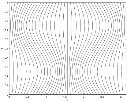
5 Numerical examples

In this section we present numerical results obtained with the numerical schemes developed in the previous sections for two one dimensional and one two dimensional examples. Our objective is to verify the stability and accuracy of those schemes.

      Example 5.1.

We first consider a one dimensional example in the form (27). The coefficients are given by

{a(x,t)=1,b(x,t)=0,c(x,t)=0,xl=0,xr=π.casesformulae-sequence𝑎𝑥𝑡1formulae-sequence𝑏𝑥𝑡0𝑐𝑥𝑡0otherwiseformulae-sequencesubscript𝑥𝑙0subscript𝑥𝑟𝜋otherwise\begin{cases}a(x,t)=1,\quad b(x,t)=0,\quad c(x,t)=0,\\ x_{l}=0,\quad x_{r}=\pi.\end{cases} (74)

The source term f(x,t)𝑓𝑥𝑡f(x,t), the initial solution, and the Dirichlet boundary conditions are chosen such that the exact solution of the IBVP is given by

uexact(x,t)=(2+sin(πt))sin(x).subscript𝑢𝑒𝑥𝑎𝑐𝑡𝑥𝑡2𝜋𝑡𝑥u_{exact}(x,t)=(2+\sin(\pi t))\sin(x). (75)

Notice that we have g(x,t)0𝑔𝑥𝑡0g(x,t)\equiv 0 for this exact solution. The mesh is chosen as

xj(t)=jπJmax+14sin(2jπJmax)sin(ωt),j=0,,Jmaxformulae-sequencesubscript𝑥𝑗𝑡𝑗𝜋subscript𝐽𝑚𝑎𝑥142𝑗𝜋subscript𝐽𝑚𝑎𝑥𝜔𝑡𝑗0subscript𝐽𝑚𝑎𝑥x_{j}(t)=\frac{j\pi}{J_{max}}+\frac{1}{4}\sin\left(\frac{2j\pi}{J_{max}}\right)\sin(\omega t),\quad j=0,...,J_{max} (76)

where the parameter ω𝜔\omega is used to control the speed of mesh movement. The trajectories of two meshes with ω=2π𝜔2𝜋\omega=2\pi and 20π20𝜋20\pi, respectively, are shown in Fig. 1.

Fig. 2(a) shows the maximum error as a function of ΔtΔ𝑡\Delta t obtained with scheme (21) + (40) (m=1𝑚1m=1) for mesh (76) (ω=2π𝜔2𝜋\omega=2\pi). In the computation, Jmaxsubscript𝐽𝑚𝑎𝑥J_{max} is taken sufficiently large (Jmax=1000subscript𝐽𝑚𝑎𝑥1000J_{max}=1000). In this case, the spatial discretization error is ignorable and the total error is dominated by the temporal discretization error. The results show the O(Δt2)𝑂Δsuperscript𝑡2O(\Delta t^{2}) behavior of the error, consistent with the theoretical prediction. They also demonstrate that the scheme is stable for all used values of ΔtΔ𝑡\Delta t.

Fig. 2(b) shows the maximum error as a function of Jmaxsubscript𝐽𝑚𝑎𝑥J_{max}. The results are obtained with m=1,2,3𝑚123m=1,2,3 and the time step size Δt=(π/Jmax)1/mΔ𝑡superscript𝜋subscript𝐽𝑚𝑎𝑥1𝑚\Delta t=(\pi/J_{max})^{1/m}, respectively. The reason ΔtΔ𝑡\Delta t is chosen this way is that the error for scheme (41) is of order O(Δt2m)+O(Δx2)𝑂Δsuperscript𝑡2𝑚𝑂Δsuperscript𝑥2O(\Delta t^{2m})+O(\Delta x^{2}), which reduces to O(Jmax2)𝑂superscriptsubscript𝐽𝑚𝑎𝑥2O(J_{max}^{-2}) with this choice of ΔtΔ𝑡\Delta t. The figure confirms that the maximum error converges quadratically for all three cases.

The numerical results obtained with scheme (21) + (40) (m=1𝑚1m=1) for a faster moving mesh ω=20π𝜔20𝜋\omega=20\pi are shown in Fig. 3. Once again, the theoretically predicted order of convergence (second order in both time and space for m=1𝑚1m=1) is observed. Interestingly, one may observe that there is a bump in the curve in Fig. 3(a). This is because for large ΔtΔ𝑡\Delta t, the fast movement of the mesh is not “felt” by the integration and this results in smaller error.

To conclude this example, we study the approximation of the boundary condition (31) with a nonhomogeneous term. Applying the collocation scheme (21) to (31) (for simplicity we keep it in the old variable), we get

u0(tn,j)=g(xl(tn,j),tn,j),uJmax(tn,j)=g(xr(tn,j),tn,j),j=1,,mformulae-sequencesubscript𝑢0subscript𝑡𝑛𝑗𝑔subscript𝑥𝑙subscript𝑡𝑛𝑗subscript𝑡𝑛𝑗formulae-sequencesubscript𝑢subscript𝐽𝑚𝑎𝑥subscript𝑡𝑛𝑗𝑔subscript𝑥𝑟subscript𝑡𝑛𝑗subscript𝑡𝑛𝑗𝑗1𝑚u_{0}({t}_{n,j})=g(x_{l}({t}_{n,j}),{t}_{n,j}),\quad u_{J_{max}}({t}_{n,j})=g(x_{r}({t}_{n,j}),{t}_{n,j}),\quad j=1,...,m (77)

where u0(t)u(x0(t),t)subscript𝑢0𝑡𝑢subscript𝑥0𝑡𝑡u_{0}(t)\approx u(x_{0}(t),t), uJmax(t)u(xJmax(t),t)subscript𝑢subscript𝐽𝑚𝑎𝑥𝑡𝑢subscript𝑥subscript𝐽𝑚𝑎𝑥𝑡𝑡u_{J_{max}}(t)\approx u(x_{J_{max}}(t),t), and tn,1,,tn,msubscript𝑡𝑛1subscript𝑡𝑛𝑚t_{n,1},...,t_{n,m} are the collocation points (cf. (20)). This has the advantage that the boundary condition is collocated at the same points as the PDE and thus can be implemented conveniently within the framework of the method of lines. On the other hand, since the boundary condition is not imposed at t=tn+1𝑡subscript𝑡𝑛1t=t_{n+1}, error may occur there and accumulate and eventually result in inaccurate computational solutions. This does not seem to be an issue for a homogeneous boundary condition. However, the situation is different when a non-homogenous boundary condition is involved.

To see this, we consider a case where the same PDE and mesh (with ω=2π𝜔2𝜋\omega=2\pi) are used but the source term, initial condition, and (non-homogeneous) boundary condition are chosen such that the exact solution is given by

uexact(x,t)=(2+sin(πt))cos(x).subscript𝑢𝑒𝑥𝑎𝑐𝑡𝑥𝑡2𝜋𝑡𝑥u_{exact}(x,t)=(2+\sin(\pi t))\cos(x). (78)

Fig. 4(a) shows the numerical results obtained with (77). It can be seen that the maximum error converges at a rate of O(Jmax1)𝑂superscriptsubscript𝐽𝑚𝑎𝑥1O(J_{max}^{-1}) for both cases m=2𝑚2m=2 and m=3𝑚3m=3, much worse than the predicted order O(Jmax2)𝑂superscriptsubscript𝐽𝑚𝑎𝑥2O(J_{max}^{-2}).

To avoid this difficulty, we consider collocating the boundary condition at the approximation points (cf. (22)), i.e.,

u0(t~n,j)=g(xl(t~n,j),t~n,j),uJmax(t~n,j)=g(xr(t~n,j),t~n,j),j=1,,m.formulae-sequencesubscript𝑢0subscript~𝑡𝑛𝑗𝑔subscript𝑥𝑙subscript~𝑡𝑛𝑗subscript~𝑡𝑛𝑗formulae-sequencesubscript𝑢subscript𝐽𝑚𝑎𝑥subscript~𝑡𝑛𝑗𝑔subscript𝑥𝑟subscript~𝑡𝑛𝑗subscript~𝑡𝑛𝑗𝑗1𝑚u_{0}(\tilde{t}_{n,j})=g(x_{l}(\tilde{t}_{n,j}),\tilde{t}_{n,j}),\quad u_{J_{max}}(\tilde{t}_{n,j})=g(x_{r}(\tilde{t}_{n,j}),\tilde{t}_{n,j}),\quad j=1,...,m. (79)

The main advantage of this approximation is that the boundary condition is now enforced at t=t~n,m=tn+1𝑡subscript~𝑡𝑛𝑚subscript𝑡𝑛1t=\tilde{t}_{n,m}=t_{n+1}. It is not difficult to show that (77) and (79) are equivalent for homogeneous Dirichlet boundary conditions but different in general. Fig. 4(b) shows the results obtained with (79). It can be seen that the second order convergence rate is recovered for all three cases. ∎

(a)Refer to caption (b)Refer to caption

Figure 1: Example 5.1: The trajectories of two meshes of 41 points for ω=2π𝜔2𝜋\omega=2\pi and ω=20π𝜔20𝜋\omega=20\pi are shown in (a) and (b), respectively.

(a) m=1𝑚1m=1Refer to caption (b) m=1,2,3𝑚123m=1,2,3Refer to caption

Figure 2: The maximum solution error for scheme (21) + (40) applied to Example 5.1 (ω=2π𝜔2𝜋\omega=2\pi). The error is plotted in (a) as a function of ΔtΔ𝑡\Delta t for Jmax=1000subscript𝐽𝑚𝑎𝑥1000J_{max}=1000 and in (b) as a function of Jmaxsubscript𝐽𝑚𝑎𝑥J_{max} for m=1𝑚1m=1 (Δt=π/JmaxΔ𝑡𝜋subscript𝐽𝑚𝑎𝑥\Delta t=\pi/J_{max}), m=2𝑚2m=2 (Δt=π/JmaxΔ𝑡𝜋subscript𝐽𝑚𝑎𝑥\Delta t=\sqrt{\pi/J_{max}}), and m=3𝑚3m=3 (Δt=π/Jmax3Δ𝑡3𝜋subscript𝐽𝑚𝑎𝑥\Delta t=\sqrt[3]{\pi/J_{max}}).

(a) m=1𝑚1m=1Refer to caption (b) m=1𝑚1m=1Refer to caption

Figure 3: The maximum error for scheme (21) + (40) (m=1𝑚1m=1) applied to Example 5.1 (ω=20π𝜔20𝜋\omega=20\pi). The error is plotted in (a) as a function of ΔtΔ𝑡\Delta t for Jmax=1000subscript𝐽𝑚𝑎𝑥1000J_{max}=1000 and in (b) as a function of Jmaxsubscript𝐽𝑚𝑎𝑥J_{max} (Δt=0.1π/JmaxΔ𝑡0.1𝜋subscript𝐽𝑚𝑎𝑥\Delta t=0.1\pi/J_{max}).

(a) BC approximation (77)Refer to caption (b) BC approximation (79)Refer to caption

Figure 4: The maximum error for scheme (21) + (40) (m=1,2,3𝑚123m=1,2,3) applied to Example 5.1 (ω=2π𝜔2𝜋\omega=2\pi) with exact solution (78). The error is plotted as a function of Jmaxsubscript𝐽𝑚𝑎𝑥J_{max} with Δt=(π/Jmax)1/mΔ𝑡superscript𝜋subscript𝐽𝑚𝑎𝑥1𝑚\Delta t=(\pi/J_{max})^{1/m}.
      Example 5.2.

We consider the one dimensional heat equation with a moving domain. The problem is in the form (27) with

{a(x,t)=1,b(x,t)=0,c(x,t)=0,xl(t)=π3sin(ωt),xr(t)=ππ3sin(ωt),casesformulae-sequence𝑎𝑥𝑡1formulae-sequence𝑏𝑥𝑡0𝑐𝑥𝑡0otherwiseformulae-sequencesubscript𝑥𝑙𝑡𝜋3𝜔𝑡subscript𝑥𝑟𝑡𝜋𝜋3𝜔𝑡otherwise\begin{cases}a(x,t)=1,\quad b(x,t)=0,\quad c(x,t)=0,\\ x_{l}(t)=\frac{\pi}{3}\sin(\omega t),\quad x_{r}(t)=\pi-\frac{\pi}{3}\sin(\omega t),\end{cases} (80)

where the parameter ω𝜔\omega is used to control the speed of the boundary movement. The source term f(x,t)𝑓𝑥𝑡f(x,t), initial solution, and Dirichlet boundary condition are chosen such that the exact solution of the IBVP is given by

uexact(x,t)=sin(π(xxl(t))xr(t)xl(t))(2+sin(πt)).subscript𝑢𝑒𝑥𝑎𝑐𝑡𝑥𝑡𝜋𝑥subscript𝑥𝑙𝑡subscript𝑥𝑟𝑡subscript𝑥𝑙𝑡2𝜋𝑡u_{exact}(x,t)=\sin\left(\frac{\pi(x-x_{l}(t))}{x_{r}(t)-x_{l}(t)}\right)(2+\sin(\pi t)). (81)

The mesh is defined as

xj=xl(t)+jJmax(xr(t)xl(t)),j=0,,Jmax.formulae-sequencesubscript𝑥𝑗subscript𝑥𝑙𝑡𝑗subscript𝐽𝑚𝑎𝑥subscript𝑥𝑟𝑡subscript𝑥𝑙𝑡𝑗0subscript𝐽𝑚𝑎𝑥x_{j}=x_{l}(t)+\frac{j}{J_{max}}(x_{r}(t)-x_{l}(t)),\quad j=0,...,J_{max}. (82)

The trajectories of two meshes with ω=2π𝜔2𝜋\omega=2\pi and 20π20𝜋20\pi are shown in Fig. 5

Recall that the mesh is treated linearly on each time interval [tn,tn+1]subscript𝑡𝑛subscript𝑡𝑛1[t_{n},t_{n+1}]. As a consequence, when the boundary of the domain is moving, the first and last mesh points, x0(t)subscript𝑥0𝑡x_{0}(t) and xJmax(t)subscript𝑥subscript𝐽𝑚𝑎𝑥𝑡x_{J_{max}}(t), generally do not coincide with the boundary points xl(t)subscript𝑥𝑙𝑡x_{l}(t) and xr(t)subscript𝑥𝑟𝑡x_{r}(t) for t(tn,tn+1)𝑡subscript𝑡𝑛subscript𝑡𝑛1t\in(t_{n},t_{n+1}); see the illustration in Fig. 6. In this situation, a more accurate approximation of the boundary conditions than (77) or (79) is needed. By expanding u(x0(t),t)𝑢subscript𝑥0𝑡𝑡u(x_{0}(t),t) and u(x1(t),t)𝑢subscript𝑥1𝑡𝑡u(x_{1}(t),t) about x=xl(t)𝑥subscript𝑥𝑙𝑡x=x_{l}(t) and u(xJmax(t),t)𝑢subscript𝑥subscript𝐽𝑚𝑎𝑥𝑡𝑡u(x_{J_{max}}(t),t) and u(xJmax1(t),t)𝑢subscript𝑥subscript𝐽𝑚𝑎𝑥1𝑡𝑡u(x_{J_{max}-1}(t),t) about xr(t)subscript𝑥𝑟𝑡x_{r}(t), we get

{(x1xl)(u0g(xl,t))(x0xl)(u1g(xl,t))=0,(xJmax1xr)(uJmaxg(xr,t))(xJmaxxr)(uJmax1g(xr,t))=0.casessubscript𝑥1subscript𝑥𝑙subscript𝑢0𝑔subscript𝑥𝑙𝑡subscript𝑥0subscript𝑥𝑙subscript𝑢1𝑔subscript𝑥𝑙𝑡0otherwisesubscript𝑥subscript𝐽𝑚𝑎𝑥1subscript𝑥𝑟subscript𝑢subscript𝐽𝑚𝑎𝑥𝑔subscript𝑥𝑟𝑡subscript𝑥subscript𝐽𝑚𝑎𝑥subscript𝑥𝑟subscript𝑢subscript𝐽𝑚𝑎𝑥1𝑔subscript𝑥𝑟𝑡0otherwise\begin{cases}(x_{1}-x_{l})(u_{0}-g(x_{l},t))-(x_{0}-x_{l})(u_{1}-g(x_{l},t))=0,\\ (x_{J_{max}-1}-x_{r})(u_{J_{max}}-g(x_{r},t))-(x_{J_{max}}-x_{r})(u_{J_{max}-1}-g(x_{r},t))=0.\end{cases} (83)

As discussed in Example 5.1, the above conditions are imposed at the approximation points, t~n,1,,t~n,msubscript~𝑡𝑛1subscript~𝑡𝑛𝑚\tilde{t}_{n,1},...,\tilde{t}_{n,m} (cf. (22)).

Numerical results obtained with scheme (21) + (40) (m=1,2,3𝑚123m=1,2,3) for ω=2π𝜔2𝜋\omega=2\pi and 20π20𝜋20\pi are shown in Figs. 7 and 8, respectively. It can be seen that the scheme is stable (the solution is bounded) and the error is of order O(Δt2m)+O(Δx2)𝑂Δsuperscript𝑡2𝑚𝑂Δsuperscript𝑥2O(\Delta t^{2m})+O(\Delta x^{2}) (m=1,2,3𝑚123m=1,2,3), consistent with the theoretical prediction. ∎

Refer to caption Refer to caption

Figure 5: Mesh trajectories of two meshes of 41 points for ω=2π𝜔2𝜋\omega=2\pi and 20π20𝜋20\pi, respectively.
Left boundary xl(t)subscript𝑥𝑙𝑡x_{l}(t)tnsubscript𝑡𝑛t_{n}tn+1subscript𝑡𝑛1t_{n+1}x0nsuperscriptsubscript𝑥0𝑛x_{0}^{n}x0n+1superscriptsubscript𝑥0𝑛1x_{0}^{n+1}t𝑡tx0(t)subscript𝑥0𝑡x_{0}(t)xl(t)subscript𝑥𝑙𝑡x_{l}(t)
Figure 6: A sketch of the boundary x=xl(t)𝑥subscript𝑥𝑙𝑡x=x_{l}(t) and the first mesh point x=x0(t)𝑥subscript𝑥0𝑡x=x_{0}(t). Generally speaking, x0(t)subscript𝑥0𝑡x_{0}(t) does not coincide with xl(t)subscript𝑥𝑙𝑡x_{l}(t) for t(tn,tn+1)𝑡subscript𝑡𝑛subscript𝑡𝑛1t\in(t_{n},t_{n+1}).

(a) m=1𝑚1m=1Refer to caption (b) m=1,2,3𝑚123m=1,2,3Refer to caption

Figure 7: The maximum error for scheme (21) + (40) (m=1,2,3𝑚123m=1,2,3) applied to Example 5.2 (ω=2π𝜔2𝜋\omega=2\pi). The error is plotted in (a) as a function of ΔtΔ𝑡\Delta t for Jmax=1000subscript𝐽𝑚𝑎𝑥1000J_{max}=1000 and in (b) as a function of Jmaxsubscript𝐽𝑚𝑎𝑥J_{max} for Δt=(π/Jmax)1/m,m=1,2,3formulae-sequenceΔ𝑡superscript𝜋subscript𝐽𝑚𝑎𝑥1𝑚𝑚123\Delta t=(\pi/J_{max})^{1/m},\;m=1,2,3.

(a): m=1𝑚1m=1Refer to caption (b): m=1𝑚1m=1Refer to caption

Figure 8: The maximum error for scheme (21) + (40) (with m=1𝑚1m=1) applied to Example 5.2 (ω=20π𝜔20𝜋\omega=20\pi). The error is plotted in (a) as a function of ΔtΔ𝑡\Delta t for Jmax=1000subscript𝐽𝑚𝑎𝑥1000J_{max}=1000 and in (b) as a function of Jmaxsubscript𝐽𝑚𝑎𝑥J_{max} for Δt=0.1π/JmaxΔ𝑡0.1𝜋subscript𝐽𝑚𝑎𝑥\Delta t=0.1\pi/J_{max}.
      Example 5.3.

The last example is a two dimensional problem in the form of IBVP (5) with

{a(x,y,t)=1,b1(x,y,t)=b2(x,y,t)=0,c(x,t)=0,Ω=(0,π)×(0,π).casesformulae-sequenceformulae-sequence𝑎𝑥𝑦𝑡1subscript𝑏1𝑥𝑦𝑡subscript𝑏2𝑥𝑦𝑡0𝑐𝑥𝑡0otherwiseΩ0𝜋0𝜋otherwise\begin{cases}a(x,y,t)=1,\quad b_{1}(x,y,t)=b_{2}(x,y,t)=0,\quad c(x,t)=0,\\ \Omega=(0,\pi)\times(0,\pi).\end{cases} (84)

The source term f(x,y,t)𝑓𝑥𝑦𝑡f(x,y,t), initial solution, and Dirichlet boundary condition are chosen such that the exact solution of the IBVP is given by

uexact(x,y,t)=(2+sin(πt))sin(x)sin(y).subscript𝑢𝑒𝑥𝑎𝑐𝑡𝑥𝑦𝑡2𝜋𝑡𝑥𝑦u_{exact}(x,y,t)=(2+\sin(\pi t))\sin(x)\sin(y). (85)

The moving mesh is generated using the coordinate transformation

x=ξ+0.2sin(2ξ)sin(2η)sin(ωt),y=η+0.2sin(2ξ)sin(2η)sin(ωt),(ξ,η)Ωformulae-sequence𝑥𝜉0.22𝜉2𝜂𝜔𝑡formulae-sequence𝑦𝜂0.22𝜉2𝜂𝜔𝑡𝜉𝜂Ωx=\xi+0.2\sin(2\xi)\sin(2\eta)\sin(\omega t),\quad y=\eta+0.2\sin(2\xi)\sin(2\eta)\sin(\omega t),\qquad(\xi,\eta)\in\Omega (86)

where the parameter ω𝜔\omega is used to control the speed of mesh movement and a rectangular mesh of (J+1)(K+1)𝐽1𝐾1(J+1)(K+1) points is used for the ξ𝜉\xi-η𝜂\eta domain. In our computation ω=2π𝜔2𝜋\omega=2\pi is used. A 41×41414141\times 41 moving mesh is shown in Fig. 9 for t=0.25𝑡0.25t=0.25 and t=0.75𝑡0.75t=0.75. The numerical results are shown in Fig. 10, which are consistent with the observations made for the 1D examples and with the theoretical prediction. ∎

(a) t=0.25𝑡0.25t=0.25Refer to caption       (b) t=0.75𝑡0.75t=0.75Refer to caption

Figure 9: A 41×41414141\times 41 moving mesh for Example 5.3 is shown for t=0.25𝑡0.25t=0.25 and t=0.75𝑡0.75t=0.75.

(a) m=1𝑚1m=1Refer to caption (b) m=1,2,3𝑚123m=1,2,3Refer to caption

Figure 10: The maximum error for scheme (21) applied to (9) with (59) and (60) for Example 5.3 (ω=2π𝜔2𝜋\omega=2\pi). The error is plotted in (a) as a function of ΔtΔ𝑡\Delta t for Jmax=Kmax=160subscript𝐽𝑚𝑎𝑥subscript𝐾𝑚𝑎𝑥160J_{max}=K_{max}=160 (Jmax=Kmax=320subscript𝐽𝑚𝑎𝑥subscript𝐾𝑚𝑎𝑥320J_{max}=K_{max}=320 was used for Δt=0.01Δ𝑡0.01\Delta t=0.01) and in (b) as a function of Jmaxsubscript𝐽𝑚𝑎𝑥J_{max} for Δt=(π/Jmax)1/m,m=1,2,3formulae-sequenceΔ𝑡superscript𝜋subscript𝐽𝑚𝑎𝑥1𝑚𝑚123\Delta t=(\pi/J_{max})^{1/m},\;m=1,2,3.

6 Conclusions and comments

In the previous sections we have developed a family of finite difference schemes for linear convection-diffusion equations on moving meshes. Those schemes can be of second and higher order in time, preserve a stability inequality, and are unconditionally stable in the sense that they impose no constraint on time step size for stability purpose. More specifically, scheme (21) has been developed for ODE system of the form (9) with property (10) by first transforming (9) into (12) and then applying the m𝑚m-point collocation scheme to the transformed system. Several finite difference discretizations for one dimensional and two dimensional convection-diffusion equations on moving meshes have been constructed and shown to satisfy property (10) (cf. Theorems 3.1 and 4.1). Numerical results presented in Section 5 verify the theoretically predicted stability and convergence order of those schemes.

Several generalizations of the current work are under investigation. It is interesting to know how the current strategy can be used for nonlinear differential equations and wave equations and how it can be combined with the method of lines for general differential equations. Moreover, it is noted that scheme (21) may not work efficiently when mass matrix M(t)𝑀𝑡M(t) is not diagonal (as in the case with finite element approximation). Development of an efficient implementation in the finite element case certainly deserves further investigations.

References

  • [1] U. Ascher, R. M. M. Mattheij, and R. D. Russell. Numerical Solution of Boundary Value Problems for Ordinary Differential Equations. Prentice-Hall, Englewood Cliffs, NJ, 1988.
  • [2] U. M. Ascher. Numerical methods for evolutionary differential equations, volume 5 of Computational Science & Engineering. Society for Industrial and Applied Mathematics (SIAM), Philadelphia, PA, 2008.
  • [3] R. E. Bank and R. F. Santos. Analysis of some moving space-time finite element methods. SIAM J. Numer. Anal., 30:1–18, 1993.
  • [4] G. Beckett and J. A. Mackenzie. Convergence analysis of finite difference approximations on equidistributed grids to a singularly perturbed boundary value problem. Appl. Numer. Math., 35:87–109, 2000.
  • [5] G. Beckett and J. A. Mackenzie. On a uniformly accurate finite difference approximation of a singularly perturbed reaction-diffusion problem using grid equidistribution. J. Comput. Appl. Math., 131:381–405, 2001.
  • [6] G. Beckett and J. A. Mackenzie. Uniformly convergent high order finite element solutions of a singularly perturbed reaction-diffusion equation using mesh equidistribution. Appl. Numer. Math., 39:31–45, 2001.
  • [7] D. Boffi and L. Gastaldi. Stability and geometric conservation laws for ALE formulations. Comput. Meth. Appl. Mech. Engrg., 193:4717–4739, 2004.
  • [8] C. J. Budd, W. Huang, and R. D. Russell. Adaptivity with moving grids. Acta Numerica, 18:111–241, 2009.
  • [9] L. Chen and J. C. Xu. Stability and accuracy of adapted finite element methods for singularly perturbed problems. Numer. Math., 109:167–191, 2008.
  • [10] C. F. Curtiss and J. O. Hirschfelder. Integration of stiff equations. Proc. US Nat. Acad. Sci., 38:235–243, 1952.
  • [11] T. Dupont. Mesh modification for evolution equations. Math. Comput., 39:85–107, 1982.
  • [12] T. F. Dupont and Y. Liu. Symmetric error estimates for moving mesh Galerkin methods for advection-diffusion equations. SIAM J. Numer. Anal., 40:914–927, 2002.
  • [13] J. A. Ferreira. On the convergence on nonrectangular grids. J. Comput. Appl. Math., 85:333–344, 1997.
  • [14] L. Formaggia and F. Nobile. A stability analysis for the arbitrary Lagrangian Eulerian formulation with finite elements. East-West J. Numer. Math., 7:105–131, 1999.
  • [15] L. Formaggia and F. Nobile. Stability analysis for second-order time accurate schemes for ALE-FEM. Comput. Meth. Appl. Mech. Eng., 193:4097–4116, 2004.
  • [16] Y. He and W. Huang. A posteriori error analysis for finite element solution of elliptic differential equations using equidistributing meshes. (arXiv:0911.0065).
  • [17] P. Henrici. Discrete Variable Methods in Ordinary Differential Equations. John Wiley, New York, 1962.
  • [18] R. G. Hindman. Generalized coordinate forms of governing fluid equations and associated geometrically induced errors. AIAA J., 20:1359–1367, 1982.
  • [19] C. W. Hirt, A. A. Amsden, and J. L. Cook. An arbitrary Lagrangian-Eulerian computing method for all flow speeds. J. Comput. Phys., 14:227–253, 1974.
  • [20] W. Huang. Convergence analysis of finite element solution of one-dimensional singularly perturbed differential equations on equidistributing meshes. International Journal of Numerical Analysis & Modeling, 2:57–74, 2005.
  • [21] W. Huang and R. D. Russell. Adaptive Moving Mesh Methods. Springer, New York, 2011. Applied Mathematical Sciences Series, Vol. 174.
  • [22] W. Huang and F. Schaeffer. An Lsuperscript𝐿{L}^{\infty} stability analysis for finite difference solution of one-dimensional convection-diffusion problems on moving meshes. J. Comput. Appl. Math., 236:3338–3348, 2012.
  • [23] N. Kopteva and M. Stynes. A robust adaptive method for a quasi-linear one-dimensional convection-diffusion problem. SIAM J. Numer. Anal., 39:1446–1467, 2001.
  • [24] Y. Liu, R. E. Bank, T. F. Dupont, S. Garcia, and R. F. Santos. Symmetric error estimates for moving mesh mixed methods for advection-diffusion equations. SIAM J. Numer. Anal., 40:2270–2291, 2003.
  • [25] J. Mackenzie. Uniform convergence analysis of an upwind finite-differnce approximation of a convection-diffusion boundary value problem on an adaptive grid. IMA J. Numer. Anal., 19:233–249, 1999.
  • [26] J. A. Mackenzie and W. R. Mekwi. An analysis of stability and convergence of a finite-difference discretization of a model parabolic PDE in 1D using a moving mesh. IMA J. Numer. Anal., 27:507–528, 2007.
  • [27] Y. Qiu and D. M. Sloan. Analysis of difference approximations to a singularly perturbed two-point boundary value problem on an adaptively generated grid. J. Comput. Appl. Math., 101:1–25, 1999.
  • [28] Y. Qiu, D. M. Sloan, and T. Tang. Numerical solution of a singularly perturbed two-point boundary value problem using equidistribution: analysis of convergence. J. Comput. Appl. Math., 116:121–143, 2000.
  • [29] P. D. Thomas and C. K. Lombard. Geometric conservation law and its application to flow computations on moving grids. AIAA J., 17:1030–1037, 1979.