Vacuum Stability and the MSSM Higgs Mass

Abstract

In the Minimal Supersymmetric Standard Model (MSSM), a Higgs boson mass of 125 GeV can be obtained with moderately heavy scalar top superpartners provided they are highly mixed. The source of this mixing, a soft trilinear stop-stop-Higgs coupling, can result in the appearance of charge- and color-breaking minima in the scalar potential of the theory. If such a vacuum exists and is energetically favorable, the Standard Model-like vacuum can decay to it via quantum tunnelling. In this work we investigate the conditions under which such exotic vacua arise, and we compute the tunnelling rates to them. Our results provide new constraints on the scalar top quarks of the MSSM.

1 Introduction

Supersymmetry predicts a scalar superpartner for every fermion in the Standard Model (SM) Martin:1997ns . While these scalar fields help to protect the scale of electroweak symmetry breaking from large quantum corrections, they can also come into conflict with existing experimental bounds. This tension is greatest for the scalar top quarks (stops). On the one hand, the stops must be heavy enough to have avoided detection in collider searches. On the other hand, smaller stop masses maximize the quantum protection of the electroweak scale Barbieri:1987fn ; Wymant:2012zp .

In the minimal supersymmetric extension of the Standard Model (MSSM), there is an additional constraint on the stops implied by the discovery of a Higgs boson with mass near $m_{h}=125\,\,{\rm GeV}$ higgs-atlas ; higgs-cms . Specifically, the stops must be heavy enough to push the (SM-like) Higgs mass up to the observed value Hall:2011aa ; Cao:2012fz . After electroweak symmetry breaking, the two gauge-eigenstate stops $\tilde{t}_{L}$ and $\tilde{t}_{R}$ mix to form two mass eigenstates, $\tilde{t}_{1}$ and $\tilde{t}_{2}$ ($m_{\tilde{t}_{1}}\leq m_{\tilde{t}_{2}}$). The corresponding mass-squared matrix in the $(\tilde{t}_{L}\;\tilde{t}_{R})^{T}$ basis is Martin:1997ns

$$\mathcal{M}_{\tilde{t}}^{2}=\left(\begin{array}[]{cc}m_{Q_{3}}^{2}+m_{t}^{2}+D_{L}&m_{t}X_{t}\\ m_{t}X_{t}^{*}&m_{U_{3}}^{2}+m_{t}^{2}+D_{R}\end{array}\right)\ ,$$ (3)

where $X_{t}=(A_{t}^{*}-\mu\cot\beta)$ is the stop mixing parameter, $m_{Q_{3},U_{3}}^{2}$ and $A_{t}$ are soft supersymmetry-breaking parameters, $\mu$ is the Higgsino mass parameter, $\tan\beta=v_{u}/v_{d}$ is the ratio of the two Higgs expectation values, and $D_{L,R}=(t^{3}-Qs^{2}_{W})m_{Z}^{2}\cos 2\beta$ are the D-term contributions. The stops generate the most important quantum corrections to the mass of the SM-like Higgs state $h^{0}$ in the MSSM. Decoupling the heavier Higgs bosons ($m_{A}\gg m_{Z}$), the $h^{0}$ mass at one-loop order is Ellis:1990nz ; Haber:1990aw ; Carena:2000dp

$$m_{h}^{2}\simeq m_{Z}^{2}\cos^{2}2\beta+\frac{3}{4\pi^{2}}\frac{m_{t}^{4}}{v^{2}}\left[\ln\left(\frac{M_{S}^{2}}{m_{t}^{2}}\right)+\frac{X_{t}^{2}}{M_{S}^{2}}\left(1-\frac{X_{t}^{2}}{12M_{S}^{2}}\right)\right]\ ,$$ (4)

where $M_{S}=(m_{Q_{3}}m_{U_{3}})^{1/2}$. The first term is the tree-level contribution and is bounded above by $m_{Z}^{2}$. The second term in Eq. (4) is the sum of one-loop top and stop contributions. This correction is essential to raising the mass of the SM-like MSSM Higgs mass to the observed value.

The contribution of the stops to the $h^{0}$ mass depends on both the mass eigenvalues and the mixing angle. Without left-right stop mixing, at least one of the stops must be very heavy, $m_{\tilde{t}}\gtrsim 5\;\,{\rm TeV}$, to obtain $m_{h}\simeq 125\,\,{\rm GeV}$ Draper:2011aa . This leads to a significant tension with the naturalness of the weak scale  Barbieri:1987fn ; Wymant:2012zp . This tension can be reduced by stop mixing, with the largest effect seen in the vicinity of the maximal mixing scenario of $X_{t}\simeq\pm\sqrt{6}M_{S}$ Casas:1994us . However, such large values of $X_{t}/M_{S}$ require a large value of $A_{t}$ (small $\mu$ is needed for naturalness Kitano:2006gv ) which can induce new vacua in the scalar field space where the stops develop vacuum expectation values (VEVs). The lifetime for tunnelling to these charge- and color-breaking (CCB) vacua must be longer than the age of the Universe to be consistent with our existence.

The existence of CCB stop vacua in the MSSM has been studied extensively  Frere:1983ag ; Gamberini:1989jw ; Claudson:1983et ; Casas:1995pd ; Falk:1995cq ; Riotto:1995am ; Kusenko:1996jn ; Casas:1996zy ; LeMouel:2001sf ; LeMouel:2001ym . Under the assumption of $SU(3)_{C}\times SU(2)_{L}\times U(1)_{Y}$ $D$-flatness, an approximate analytic condition for the non-existence of a CCB stop vacuum is Claudson:1983et ; Casas:1995pd

$$A_{t}^{2}<3(m_{Q_{3}}^{2}+m_{U_{3}}^{2}+m_{2}^{2})\ ,$$ (5)

where $m_{2}^{2}=m_{H_{u}}^{2}+|\mu|^{2}$ and $m_{H_{u}}^{2}$ is the $H_{u}$ soft mass squared parameter. Generalizations to less restrictive field configurations Casas:1995pd ; Casas:1996zy ; LeMouel:2001sf ; LeMouel:2001ym and studies of the thermal evolution of such vacua Carena:1996wj ; Cline:1999wi ; Patel:2013zla have been performed as well. Relaxing the requirement of absolute stability of our electroweak vacuum and demanding only that the tunnelling rate to the CCB vacua is sufficiently slow provides a weaker bound. The tunnelling rate was computed in Ref. Kusenko:1996jn , where the net requirement for metastability was expressed in terms of the empirical relation

$$A_{t}^{2}+3\mu^{2}\lesssim 7.5(m_{Q_{3}}^{2}+m_{U_{3}}^{2})\ .$$ (6)

In this work we attempt to update and clarify the stability and metastability bounds on the parameters in the stop sector of the MSSM. We expand upon the previous body of work by investigating the detailed dependence of the limits on the underlying set of stop parameters. Furthermore, we relate our revised limits to recent Higgs and stop search results at the LHC.

The outline of this paper is as follows. In Section 2 we specify the ranges of MSSM parameters and field configurations to be considered. Next, in Section 3 we investigate the necessary conditions on the underlying stop and Higgs parameters for the scalar potential to be stable or safely metastable. We then compare the constraints from metastability to existing limits on the MSSM stop parameters from the Higgs mass in Section 4, as well as to direct and indirect stop searches in Section 5. Finally, we conclude in Section 6. Some technical details related to our tunnelling calculation are expanded upon in the Appendix.

2 Parameters and Potentials 

In our study, we consider only variations in the scalar fields derived from the superfields $Q_{3}\to(\tilde{t}_{L},\tilde{b}_{L})^{T}$, $U^{c}_{3}\to\tilde{t}_{R}^{*}$, $H_{u}\to(H_{u}^{+},H_{u}^{0})$, and $H_{d}\to(H_{d}^{0},H_{d}^{-})$. To make this multi-dimensional space more tractable, we further restrict ourselves to configurations where $\tilde{b}_{L}=H_{u}^{+}=H_{d}^{-}=0$ and the remaining fields (and MSSM parameters) are real-valued. Previous studies of CCB vacua in the stop direction suggest that this condition is not overly restrictive Casas:1995pd .

2.1 Scalar Potential

Under these assumptions, the tree-level scalar potential becomes

$$V_{\mathrm{tree}}=V_{2}+V_{3}+V_{4}$$ (7)

where

$$V_{2} = (m_{H_{u}}^{2}+|\mu|^{2})(H_{u}^{0})^{2}+(m_{H_{d}}^{2}+|\mu|^{2})(H_{d}^{0})^{2}-2bH_{u}^{0}H_{d}^{0}+m_{Q_{3}}^{2}\tilde{t}_{L}^{2}+m_{U_{3}}^{2}\tilde{t}_{R}^{2}$$ (8)

$$V_{3} = 2y_{t}(A_{t}H_{u}^{0}-\mu\,H_{d}^{0})\,\tilde{t}_{L}\tilde{t}_{R}$$ (9)

$$V_{4} = y_{t}^{2}\left[\tilde{t}_{L}^{2}\tilde{t}_{R}^{2}+\tilde{t}_{L}^{2}(H_{u}^{0})^{2}+\tilde{t}_{R}^{2}(H_{u}^{0})^{2}\right]+V_{D}\ ,$$ (10)

with

$$V_{D}=\frac{{g^{\prime}}^{2}}{8}\left[(H_{u}^{0})^{2}-(H_{d}^{0})^{2}+\frac{1}{3}\tilde{t}_{L}^{2}-\frac{4}{3}\tilde{t}_{R}^{2}\right]^{2}+\frac{g^{2}}{8}\left[-(H_{u}^{0})^{2}+(H_{d}^{0})^{2}+\tilde{t}_{L}^{2}\right]^{2}+\frac{g_{3}^{2}}{6}\left(\tilde{t}_{L}^{2}-\tilde{t}_{R}^{2}\right)^{2}\ .$$ (11)

In writing this form, we have implicitly assumed that the stops are aligned (or anti-aligned) in $SU(3)_{C}$ space, so that $\tilde{t}_{L}$ and $\tilde{t}_{R}$ may be regarded as the magnitudes of these color vectors (up to a possible sign). It is not hard to show that such an alignment maximizes the likelihood of forming a CCB minimum.

In our analysis of metastability, we use the tree-level potential of Eq. (7) with the parameters in it taken to be their $\overline{\mathrm{DR}}$ running values defined at the scale $M_{S}$. However, we also compare our metastability results to a full two-loop calculation of the Higgs boson mass. While this is a mismatch of orders, we do not expect that including higher order corrections will drastically change our metastability results for two reasons. First and most importantly, the formation of CCB vacua is driven by the trilinear stop coupling $A_{t}$, which is already present in the tree-level potential. Second, when a CCB vacuum exists, the large stop Yukawa coupling $y_{t}\sim 1$ implies that it typically occurs at field values on the order of $M_{S}$ Casas:1995pd . Thus we do not expect large logarithmic corrections from higher orders.

Including higher-order corrections in the tunnelling analysis is also challenging for a number of technical reasons. Turning on multiple scalar fields, the mass matrices entering the Coleman-Weinberg corrections to the effective potential become very complicated and multi-dimensional Cline:1999wi . These corrections can be absorbed into running couplings by an appropriate field-dependent choice of the renormalization scale Gamberini:1989jw . In doing so, however, the otherwise field-independent corrections to the vacuum energy (which are not included in the Coleman-Weinberg potential) develop a field dependence. These vacuum energy corrections must be included to ensure the net scale independence of the effective potential Kastening:1991gv ; Ford:1992mv . Beyond the effective potential, kinetic corrections (i.e. derivative terms in the effective action) will also be relevant for the non-static tunnelling configurations to be studied. Furthermore, the effective potential and the kinetic corrections are both gauge dependent Jackiw:1974cv ; Patel:2011th . The gauge dependence of the effective potential can be shown to cancel on its own for static points Nielsen:1975fs ; Fukuda:1975di . However, to ensure the gauge invariance of the non-static tunnelling configuration and thus the decay rate, kinetic corrections must be included as well Metaxas:1995ab ; Garny:2012cg . For these various reasons, we defer an investigation of higher-order corrections to metastability to a future work.

2.2 Parameter Ranges

Without loss of generality, we may redefine $H_{u}^{0}$ and $H_{d}^{0}$ such that $b$ and $H_{u}^{0}$ are both positive. This ensures that the unique SM-like vacuum (with $\tilde{t}_{L}=\tilde{t}_{R}=0)$ has $\tan\beta=\langle H_{u}^{0}\rangle/\langle H_{d}^{0}\rangle>0$, and thus $\langle H_{d}^{0}\rangle>0$ as well. By demanding that a local SM-like vacuum exists, $b$, $m_{H_{u}}^{2}$, and $m_{H_{d}}^{2}$ can be exchanged in favour of $v=\sqrt{\langle H_{u}^{0}\rangle^{2}+\langle H_{u}^{0}\rangle^{2}}$, $\tan\beta$, and the pseudoscalar mass $m_{A}$:

$$b = \frac{1}{2}m_{A}^{2}\sin({2\beta})$$ (12)

$$m_{H_{u}}^{2} = -\mu^{2}+m_{A}^{2}\cos^{2}\!\beta+\frac{1}{2}m_{Z}^{2}\cos(2\beta)$$ (13)

$$m_{H_{d}}^{2} = -\mu^{2}+m_{A}^{2}\sin^{2}\!\beta-\frac{1}{2}m_{Z}^{2}\cos(2\beta)\ .$$ (14)

Moving out in the stop directions, we may also redefine $\tilde{t}_{L}$ and $\tilde{t}_{R}$ such that $\tilde{t}_{L}$ is positive.

The parameter ranges we investigate are motivated by existing bounds on the MSSM and naturalness. We typically scan over $(m_{Q_{3}}^{2},X_{t})$ while holding other potential parameters fixed. We also consider discrete variations in $m_{U_{3}}^{2}/m_{Q_{3}}^{2}$, $\tan\beta$, $\mu$, and $m_{A}$. The corresponding ranges are specified in Table 1. For the remaining supersymmetry breaking parameters, we choose $m_{\tilde{f}}=2\,\,{\rm TeV}$ and $A_{f}=0$ for all sfermions other than the stops, as well as $M_{1}=300\,\,{\rm GeV}$, $M_{2}=600\,\,{\rm GeV}$, and $M_{3}=2\,\,{\rm TeV}$. To interface with the Higgs mass calculation, we take these to be running $\overline{\mathrm{DR}}$ values defined at the input scale $M_{S}=(m_{Q_{3}}m_{U_{3}})^{1/2}$. We also use running $\overline{\mathrm{DR}}$ values of $y_{t}$, $g^{\prime}$, $g$, and $g_{3}$ at scale $M_{S}$ when evaluating the potential.

Parameter	Values
$|m_{Q_{3}}|$	$[300,3000]\;\,{\rm GeV}$
$m_{Q_{3}}^{2}/m_{U_{3}}^{2}$	${0.3\,,1,\,3}$
$X_{t}$	$[-10,10]\times|m_{Q_{3}}|$
$\mu$	${150,\,300,\,500}\;\,{\rm GeV}$
$m_{A}$	${1000}\;\,{\rm GeV}$
$\tan\beta$	${5,\,10,\,30}$

Table 1: MSSM scalar potential parameter scan ranges. The values of other parameters to be considered are described in the text.

.

3 Limits From Vacuum Stability 

A necessary condition on the viability of any realization of the MSSM is that the lifetime of the SM-like electroweak vacuum at zero temperature be longer than the age of the Universe. This will certainly be the case if the electroweak vacuum is a global minimum, and it can also be true in the presence of a deeper CCB minimum provided the tunnelling rate is sufficiently small. More stringent conditions can be derived for specific cosmological histories Cline:1999wi . While color-broken phases in the early Universe can have interesting cosmological implications, such as for baryogenesis Carena:1996wj ; Cline:1999wi ; Patel:2013zla , we focus exclusively on the history-independent $T=0$ metastability condition.

3.1 Existence of a CCB Vacuum

The first step in a metastability analysis is to determine whether a CCB minimum exists. Such minima are induced by a competition between the trilinear $A$ and quartic couplings $\lambda$ in the potential, and one generally expects $\langle\phi\rangle_{\mathrm{CCB}}\sim A/\lambda$ Casas:1995pd . We use this expectation as a starting point for a numerical minimization of the potential, Eq. (7), employing the minimization routine Minuit2 James:1975dr . For every MSSM model, we choose the starting point to be $\langle\phi_{i}\rangle_{\mathrm{CCB}}=\xi_{i}A_{t}$, where $\xi_{i}\in[-1,1]$ is chosen randomly. The global CCB vacua we find are generally unique, up to our restrictions of $H_{u}^{0},\,\tilde{t}_{L}\geq 0$. If no global CCB minimum is found, the minimization is repeated several times with new $\xi_{i}$ values. If the global minimum turns out to be the EW vacuum, the model is considered to be Standard Model-like (SML).

3.2 Computing the Tunnelling Rate

When a deeper CCB vacuum is found, the decay rate of the SML vacuum is computed using the Callan-Coleman formalism Coleman:1977py ; Callan:1977pt , where the path integral is evaluated in the semi-classical approximation. The decay rate per unit volume is given by

$$\Gamma/V=C\exp(-B/\hbar)\ ,$$ (15)

where $B=S_{E}[\bar{\bm{\mathbf{\phi}}}]$ is the Euclidean action evaluated on the bounce solution $\bar{\bm{\mathbf{\phi}}}$. The bounce is $O(4)$-symmetric, depending only on $\rho=\sqrt{t^{2}+\bm{\mathbf{x}}^{2}}$, and satisfies the classical equations of motion subject to the boundary conditions $\partial_{\rho}\bar{\bm{\mathbf{\phi}}}|_{\rho=0}=0$ and $\lim_{\rho\to\infty}\bar{\bm{\mathbf{\phi}}}=\bm{\mathbf{\phi}}_{+}$, where $\bm{\mathbf{\phi}}_{+}$ is the false-vacuum field configuration. The pre-exponential factor $C$ is obtained from fluctuations around the classical bounce solution. It is notoriously difficult to compute Dunne:2005rt ; Min:2006jg , and is therefore usually estimated on dimensional grounds Weinberg:1992ds . We use

$$[C]=M^{4}\;\Rightarrow C=(100\;\,{\rm GeV})^{4}\ .$$ (16)

The metastability of the SM-like vacuum then requires

$$\Gamma^{-1}\gtrsim t_{0}\;\Rightarrow\;B/\hbar\gtrsim 400,$$ (17)

where $t_{0}=13.8\;\mathrm{Gyr}$ is the age of the universe. Our choice of scale for $C$ corresponds to the SM-like vacuum, and provides a reasonable lower bound on $C$. Larger values of $C$ would increase the decay rate, implying that the limits we derive are conservative.

Finding the bounce $\bar{\bm{\mathbf{\phi}}}$ is straightforward in one field dimension, since the equation of motion can be solved by the shooting method. This method reduces the problem to a root-finding task for the correct boundary conditions and relies on the unique topology of the one-dimensional field space. Unfortunately, this strategy becomes intractable with more than one field dimension. Several methods of solving the multi-field bounce equation of motion have been proposed Kusenko:1995jv ; Cline:1999wi ; Konstandin:2006nd ; Park:2010rh . In the present analysis we use the public code CosmoTransitions Wainwright:2011kj .

CosmoTransitions (CT) implements a path deformation method similar to the that suggested in Ref. Cline:1999wi . Once a pair of local minima are specified, CT fixes a one-dimensional path between them in the field space. Along this path, the one-dimensional bounce solution can be computed using the shooting method. In Appendix A, we show that the action computed from the bounce solution for any such fixed path is necessarily greater than or equal to the unconstrained bounce action. The fixed path in field space is then deformed by minimizing a set of perpendicular gradient terms to be closer to the true bounce path through the field space. This procedure is iterated until convergence is reached. We exclude any points where CT fails to converge.

This path deformation approach has several advantages over other methods. Here, the bounce equation of motion is solved directly, while many other approaches involve minimization of a discretized action as part of the procedure. This is numerically costly, since one needs both a fine lattice spacing to evaluate derivatives accurately, and a large $\rho$ domain to accommodate the boundary condition at infinity. Path deformation involves no discretization or large-scale minimization. As a result CosmoTransitions is quite fast for our four-field tunnelling problem.

We also cross check the CT results in two ways. First, we have compared CT to the discretized action methods of Refs. Konstandin:2006nd ; Park:2010rh for a set of special cases, and we generally find agreement between these approaches. Second, we also compute the bounce action independently along the optimal path determined by CT, allowing us to estimate the numerical uncertainty on the bounce. Finally, let us emphasize once more that even if the path determined by CT is not the true tunnelling trajectory, our result in Appendix A implies that it still provides an upper bound on the bounce action, and thus a lower bound on the tunnelling rate.

We note that recently a new program, Vevacious Camargo-Molina:2013qva , has been released that can also be used to study metastability in field theories with many scalar fields. While we do not use this code, we share some similarities with their approach in that we both employ Minuit for potential minimization and CT for tunneling rates. However, as mentioned above, we also carried out extensive independent checks of the tunneling calculation.

3.3 Results and Comparison

We begin by presenting our limits from metastability alone, without imposing any other constraints such as the Higgs mass requirement. This allows for a direct comparison with the results of Ref. Kusenko:1996jn . In Fig. 1 we show a scan over $X_{t}$ and $m_{Q_{3}}^{2}$ while keeping fixed $m_{A}=1000\;\,{\rm GeV}$, $\tan\beta=10$, $\mu=300\;\,{\rm GeV}$, and $m_{U_{3}}^{2}/m_{Q_{3}}^{2}=1$. Every point shown is a model with a global CCB vacuum. The red points have a tunnelling action $B/\hbar<400$, and are therefore unstable on cosmological time scales. The blue points have a metastable SM-like vacuum with $B/\hbar>400$. Also shown in the figure is the analytic bound (green dashed line) of Eq. (5), and the empirical result (black dotted line) from Ref. Kusenko:1996jn given in Eq. (6).

The shape of the regions shown in Fig. 1 can be understood simply. As expected, the existence of a CCB vacuum requires a large value of $A_{t}/M_{S}$. The cutoff at the upper-left diagonal edge corresponds to the absence of a CCB vacuum. Above and to the left of this boundary, the SML minimum is a global one and the EW vacuum can be absolutely stable. There is also a lack of points below a lower-right diagonal edge. Here, one of the physical stops becomes tachyonic, and the SML vacuum disappears altogether. At low values of $A_{t}^{2}$, we see that the CCB region is squeezed between the SML region (on the left) and the tachyonic stop region (on the right), giving rise to the cutoff seen in the lower left corner.

It is apparent from Fig. 1 that we find much more restrictive metastability bounds on the MSSM than the empirical relation of Eq. (6) from Ref. Kusenko:1996jn . We also see that the analytic bound of Eq. (5) tends to underestimate the existence of CCB vacua, and that it accidentally lines up fairly well with the lower boundary of metastability. It is not clear why our results should be so much more restrictive than those found in Ref. Kusenko:1996jn , but we are confident that the path deformation method of CT (and our several cross-checks) gives a robust upper bound on the bounce action. We find qualitatively similar results for the other parameters ranges described in Table 1. The quantitative results for these ranges will be presented in more detail below in the context of the Higgs mass.

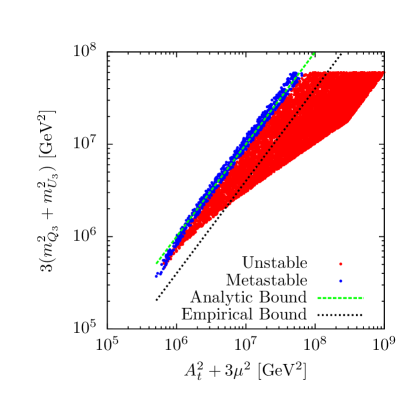
Figure 1: Limits from metastability and the existence of a local SM-like (SML) vacuum alone for $\tan\beta=10$, $\mu=300\,\,{\rm GeV},$ $m_{A}=1000\,\,{\rm GeV}$, and $m_{U_{3}}^{2}=m_{Q_{3}}^{2}$. All points shown have a global CCB minimum and a local SML minimum. The red points are dangerously unstable, while the blue points are consistent with metastability. The green dashed line is the analytic bound of Eq. (5) and the black dotted line corresponds to Eq. (6), the empiricial bound from Ref. Kusenko:1996jn . The values of the other MSSM parameters used here are described in the text.

4 Implications for the MSSM Higgs Boson

As discussed in the Introduction, there is a significant tension in the MSSM between obtaining the observed Higgs boson mass and keeping the stops relatively light. This tension is reduced when the stops are strongly mixed. To obtain such mixing, large values of $X_{t}$ are needed. We have just seen that large values of $X_{t}$ can lead to dangerous CCB minima. In this section we compare the relative conditions imposed by each of these requirements.

To calculate the physical $h^{0}$ Higgs boson mass, we use FeynHiggs 2.9.5 Heinemeyer:1998yj . We also use this program together with SuSpect 2.43 Djouadi:2002ze to compute the mass spectrum of the MSSM superpartners. As inputs, we take $m_{t}^{\mathrm{pole}}=173.1\,\,{\rm GeV}$ and $\alpha_{s}(m_{Z})=0.118$ Beringer:1900zz . Our results are exhibited in terms of variations on the fiducial MSSM parameters $\tan\beta=10$, $\mu=300\,\,{\rm GeV},$ $m_{A}=1000\,\,{\rm GeV}$, and $m_{U_{3}}^{2}=m_{Q_{3}}^{2}$. The other MSSM parameters are taken as in Section 2.2.

In Fig. 2 we show points in the $X_{t}$-$M_{S}$ plane (where $M_{S}=(m_{Q_{3}}m_{U_{3}})^{1/2}$) that produce a Higgs mass in the range $123\;\,{\rm GeV}<m_{h}<127\;\,{\rm GeV}$. All other parameters are set to their fiducial values described above. The pink (blue) region are models with a global SML (CCB) vacuum. The red points are excluded by metastability. The dashed lines show the approximate CCB condition of Eq. (5), the empirical limit of Eq. (6), and our own attempt at an empirical limit on metastability to be discussed below. The requirement of metastability cuts off a significant portion of the allowed range at very large $|X_{t}|$. Also shown are contours of constant $m_{\tilde{t}_{1}}$, the lightest stop mass (grey dot-dashed lines).

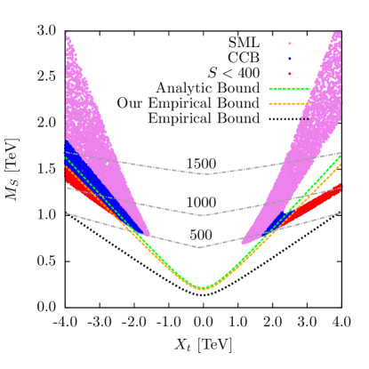
Figure 2: Metastability bounds relative to the MSSM Higgs mass. The colored bands contain models for which $123\;\,{\rm GeV}<m_{h}<127\;\,{\rm GeV}$. Pink models have an absolutely stable SML vacuum, blue points have a global CCB minimum, while red points are unstable on cosmological time scales. The green dashed line is the analytic bound of Eq. (5) and the black dotted line is Eq. (6). The orange dashed line is an approximate empirical bound discussed in Appendix B. The grey dot-dashed contours are lines of constant lightest stop mass (in GeV). MSSM parameters used here are described in the text.

In Fig. 3 we show the additional dependence of the Higgs mass and the metastability bounds on other relevant MSSM parameters. All parameters are set to their fiducial values except for those we vary one at a time. In the top row we show results for $\tan\beta=5~{}(30)$ on the left (right). Reducing $\tan\beta$ decreases the tree-level contribution to the MSSM Higgs mass, and so larger values of $M_{S}$ are needed to raise $m_{h}$ to the observed range. These larger values also lead to shallower CCB minima and lower tunnelling rates. Larger values of $\tan\beta$ do not appear to differ much from $\tan\beta=10$.

In the middle row of Fig. 3 we show results for $\mu=150~{}(500)\ ,\,{\rm GeV}$ on the left (right). We do not see a large amount of variation in the exclusions from metastability, which is not surprising given that generally have $X_{t}\simeq A_{t}\gg\mu$. Setting $\mu=-300\,\,{\rm GeV}$ also produces very similar results.

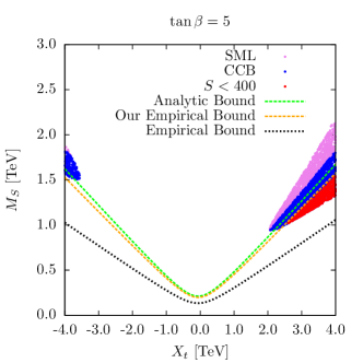
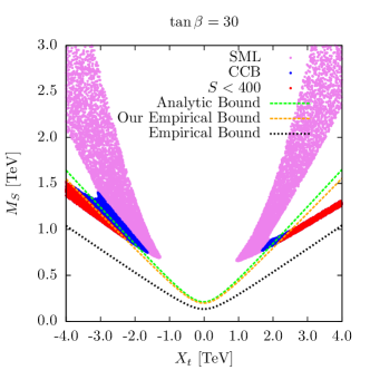
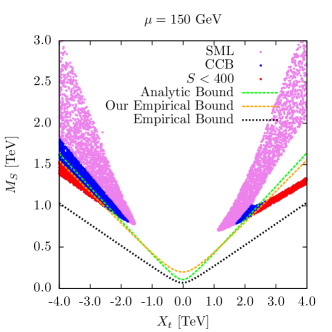
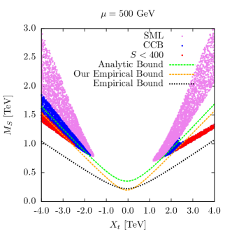
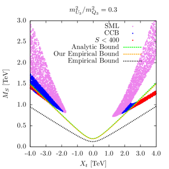
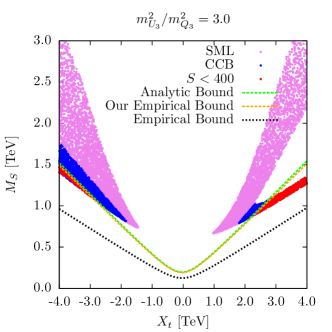
Figure 3: Metastability with the correct Higgs mass, $123<m_{h}<127\,\,{\rm GeV}$. The labelling is the same as in Fig. 2, and the relevant MSSM parameter parameters are varied one at a time as summarized in Table 1.

In the bottom row of Fig. 3 we show the same metastability limits for $m_{U_{3}}^{2}/m_{Q_{3}}^{2}=0.3~{}(3.0)$ on the left (right). For these unequal values, there is a tension between minimizing the quadratic terms in the potential and reducing the quartic terms through $SU(3)_{c}$ $D$-flatness. Unequal squark VEVs also tend to reduce the effective trilinear term. Together, these effects reduce the metastability constraint somewhat, but do not eliminate it.

In summary, the constraint imposed by CCB metastability rules out a significant portion of the MSSM stop parameter space that can produce a Higgs mass near the observed value. The limits are strongest on the outer branches at large $|X_{t}|$. Varying other MSSM parameters within the restricted ranges we have considered does not drastically alter this result. By comparison, the empirical bound from Ref. Kusenko:1996jn does not rule out any of the stop parameter space consistent with the Higgs mass.

As a synthesis of these results, we have attempted to obtain an improved empirical bound on stop-induced metastability. We find the approximate limit

$$A_{t}^{2}\lesssim\left(3.4+0.5\frac{|1-r|}{1+r}\right)m_{T}^{2}+60\,m_{2}^{2}\ ,$$ (18)

where $m_{T}^{2}=(m_{Q_{3}}^{2}+m_{U_{3}}^{2})$, $m_{2}^{2}=(m_{H_{u}}^{2}+\mu^{2})$, and $r=m_{U_{3}}^{2}/m_{Q_{3}}^{2}$. Let us emphasize that this limit is very approximate and only applies to smaller values of $\mu$, larger values of $m_{A}$, moderate $\tan\beta$, and $r$ not too different from unity. Details on the derivation of this bound are given in Appendix B.

5 Comparison to Other Stop Constraints

The metastability conditions we find exclude parameter regions with large stop mixing. This mixing can produce one relatively light stop mass eigenstate as well as a significant mass splitting between the members of the $\widetilde{Q}_{3}$ sfermion doublet. These features are constrained indirectly by electroweak and flavor measurements, as well as by direct searches for a light stop. In this section we compare these additional limits to the bounds from metastability.

5.1 Precision Electroweak and Flavor

The most important electroweak constraint on light stops comes from $\Delta\rho$, corresponding to the shift in the $W$ mass relative to the $Z$. In the context of highly mixed stops motivated by the Higgs mass, this effect has been studied in Refs. Barger:2012hr ; Espinosa:2012in . We have computed the shift $\Delta\rho$ due to stops and sbottoms using SuSpect 2.43 Djouadi:2002ze , which applies the one-loop results contained in Refs. Drees:1990dx ; Heinemeyer:2004gx . With a Higgs mass of $m_{h}\simeq 125\,\,{\rm GeV}$, the preferred range is $\Delta\rho=(4.2\pm 2.7)\times 10^{-4}$  Barger:2012hr .

Supersymmetry can also contribute to flavor-mixing. Assuming only super-CKM squark mixing (or even minimal flavor violation D'Ambrosio:2002ex ), the most constraining flavor observable is frequently the branching ratio $\mathrm{BR}(B\to X_{s}\gamma)$. It receives contributions in the MSSM from stop-chargino and top-$H^{+}$ loops. These contributions tend to cancel each other such that the cancellation would be exact in the supersymmetric limit Ciuchini:1998xy . With supersymmetry breaking, the result depends on the stop masses and mixings, $\tan\beta$, $\mu$, and the pseudoscalar mass $m_{A}$. Constraints on light stops from $\mathrm{BR}(B\to X_{s}\gamma)$ were considered recently in Refs. Heinemeyer:2011aa ; Espinosa:2012in . The SM prediction is $\text{BR}(B\to X_{s}\gamma)=(3.15\pm 0.23)\times 10^{-4}$ Grzadkowski:2008mf , while a recent Heavy Flavor Averaging Group compilation of experimental results finds $\text{BR}(B\to X_{s}\gamma)=(3.55\pm 0.24\pm 0.09)\times 10^{-4}$ Amhis:2012bh . We have investigated the limit from $\mathrm{BR}(B\to X_{s}\gamma)$ and other flavor observables using SuperIso 3.3 Arbey:2009gu assuming only super-CKM flavor mixing.

In Fig. 4, we show the exclusions from flavor and electroweak bounds for model points with $123\;\,{\rm GeV}<m_{h}<127\;\,{\rm GeV}$ for $\tan\beta=10$, and $m_{A}=1000\,\,{\rm GeV}$, $\mu=300\,\,{\rm GeV}$, and $m_{Q_{3}}^{2}=m_{U_{3}}^{2}$ in the $X_{t}\!-\!m_{Q_{3}}$ plane. We impose the generous $2\sigma$ constraints $\Delta\rho\in[-1.2,9.4]\times 10^{-4}$ and $\mathrm{BR}(B\to X_{s}\gamma)\in[2.86,4.24]\times 10^{-4}$ and show them together with the metastability constraint from the previous Section. The green points show the regions excluded by $\Delta\rho$ while the orange points show those excluded by $\mathrm{BR}(B\to X_{s}\gamma)$.

The exclusion due to $\Delta\rho$ can be understood in terms of the large stop mixing induced by $X_{t}$, which generates a significant splitting between the mass eigenstates derived from the $\widetilde{Q}_{3}=(\tilde{t}_{L},\tilde{b}_{L})^{T}$ $SU(2)_{L}$ doublet. This constraint depends primarily on the stop parameters, and is mostly insensitive to variations in $\mu$, $m_{A}$, and $\tan\beta$. While this bound overlaps significantly with the limit from metastability, there are regions where only one of the two constraints applies. The limits from $\Delta\rho$ are also weaker for $m_{Q_{3}}^{2}>m_{U_{3}}^{2}$.

Limits from $\text{BR}(B\to X_{s}\gamma)$ are less significant for this set of fiducial parameters with a moderate value of $\tan\beta$. However, this branching fraction depends significantly on $\mu$, $m_{A}$, and $\tan\beta$, and the limit can be much stronger or much weaker depending on the specific values of these parameters. We do not attempt to delineate the acceptable parameter regions, but we do note that the constraint from metastability can rule out an independent region of the parameter space.

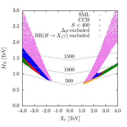
Figure 4: Points in the $X_{t}\!-\!m_{Q_{3}}$ plane with $123\;\,{\rm GeV}<m_{h}<127\;\,{\rm GeV}$ as well as exclusions from metastability (red points) from precision electroweak $\Delta\rho$ (green points) and flavor $\mathrm{BR}(B\to X_{s}\gamma)$ (orange points). The MSSM parameters used are the same as in Fig. 2.

5.2 Direct Stop Searches

Stops have been searched for at the LHC in a diverse range of final states, and these studies rule out stop masses up to 200-600​  GeV, depending on how the stop decays (see e.g. Refs. Aad:2013ija ; ATLAS:2013ama ; Chatrchyan:2013xna ; CMS:stp ). While the large stop mixing that occurs in the region excluded by metastability considerations can produce lighter stops, the stop masses in this dangerously metastable region are not necessarily light, as can be seen in Fig. 2. Thus, metastability excludes parameter ranges beyond existing direct searches.

Note as well that metastability does not place a lower bound on the mass of the lightest stop. For example, a very light state can be obtained for $m_{U_{3}}^{2}\ll m_{Q_{3}}^{2}$ and $X_{t}=0$. This scenario is not constrained by metastability, and can generate a SM-like Higgs boson mass consistent with observations for sufficiently large values of $m_{Q_{3}}^{2}$ Carena:2008rt .

Our results also have implications for future stop searches and measurements. Should a pair of stops be discovered, a variety of methods can be used to determine the underlying parameters in the stop mass matrix through precision measurements at the LHC Hisano:2002xq ; Rolbiecki:2009hk ; Blanke:2010cm ; Perelstein:2012fc or a future $e^{+}e^{-}$ collider Berggren:1999ss ; Boos:2003vf ; Perelstein:2012fc . If these stop parameters turn out to lie within the dangerously unstable region, corresponding to larger values of $|X_{t}|$, we can conclude that new physics beyond the MSSM must be present.

5.3 Stop Bound States

An additional phenomenon that can potentially occur in the MSSM when $A_{t}$ is very large is the formation of a $\tilde{t}_{L}\tilde{t}_{R}^{*}$ bound state through the exchange of light Higgs bosons Giudice:1998dj ; Hernandez:2001mi . Such a state could have the quantum numbers of a Higgs field and mix with the MSSM Higgs fields to participate in electroweak symmetry breaking Giudice:1998dj ; Hernandez:2001mi ; Cornwall:2012ea ; Pearce:2013yja . If this occurs, our results on the metastability of the MSSM may no longer apply. Calculating the critical value of $A_{t}$ for when a bound state arises is very challenging, but under a set of reasonable approximations Ref. Cornwall:2012ea finds that it requires $A_{t}/M_{S}\gtrsim 15$. While this lies beyond the region considered in the present work, it is conceivable that a full numerical analysis would yield a lower critical value for this ratio.

6 Conclusions 

In this work we have investigated the limits on the stop parameter space imposed by vacuum stability considerations. A SM-like Higgs boson with a mass of $\sim 125\;\,{\rm GeV}$ in the MSSM points to a particular region of the parameter space if naturalness of the EW scale is desired. In this regime, the two stop gauge eigenstates are highly mixed, and this can induce the appearance of charge- and color-breaking minima in the scalar potential. Quantum tunnelling to these vacua can destabilize the electroweak ground-state.

We have studied the conditions under which stop mixing can induce CCB vacua and we have computed the corresponding tunnelling rates. We find that metastability provides an important constraint on highly-mixed stops. We have also considered constraints from flavor and precision electroweak observables and direct stop searches, which are sensitive to a similar region of the MSSM parameter space. Metastability provides new and complimentary limits, with a different dependence on the underlying parameter values.

The metastability limits we have derived provide a necessary condition on the MSSM. They apply for both standard and non-standard cosmological histories. Let us emphasize, however, that the MSSM parameter points that we have found to be consistent with stop-induced CCB limits may still be ruled out by more general stability considerations, such as configurations with more non-zero scalar fields. Fortunately, our own SML vacuum appears to be at least safely metastable.

Note Added: While this manuscript was in preparation, two other works considering limits on the MSSM from vacuum stability appeared Camargo-Molina:2013sta ; Chowdhury:2013dka . A preliminary version of the present results was also posted as a contribution to a conference proceedings Blinov:2013uda . We study a different region of MSSM parameter space than Ref. Camargo-Molina:2013sta , but we do have significant overlap with Ref. Chowdhury:2013dka . Our results are substantially in agreement with Ref. Chowdhury:2013dka , although our exclusions from metastability extend to larger values of $X_{t}$. We suspect that this difference is due to slightly different choices of parameters as well as variations in the outputs of the spectrum generators that were used in our respective analyses.

Appendix A Minimality of the Action Under Path Deformations

In this appendix we show that fixing a path in field space connecting two vacua and computing the one-dimensional bounce action along that path provides on upper bound on the bounce action for tunnelling between those vacua. Equivalently, the bounce solution of the Euclidean action is a minimum of the action with respect to deformations of fixed, one-dimensional paths in the field space. The implication of this result is that the path deformation method of CosmoTransitions (CT) Wainwright:2011kj is guaranteed to provide at least an upper bound on the tunnelling lifetime.

Recall that the multi-field bounce solution $\bar{\bm{\mathbf{\phi}}}(\rho)$, $\rho=\sqrt{t^{2}+\bm{\mathbf{x}}^{2}}$, of the Euclidean action is an $\mathcal{O}(4)$-symmetric solution of the classical equations of motion subject to the boundary conditions

$$\partial_{\rho}\bar{\bm{\mathbf{\phi}}}(\rho=0)=0\ ,~{}~{}~{}~{}~{}\lim_{\rho\to\infty}{\bar{\bm{\mathbf{\phi}}}}=\bm{\mathbf{\phi}}_{+}\ ,$$ (19)

where $\bm{\mathbf{\phi}}_{+}$ is the metastable vacuum configuration. The bounce action is just the Euclidean action evaluated on the bounce solution.

Let us now restate our claim more precisely. The bounce solution is an element of the set of parametric curves on $\mathbb{R}^{F}$, where $F$ is the number of scalar fields. Any path $\bm{\mathbf{\phi}}(\rho)$ in this set can be written in terms of a unit speed curve $\bm{\mathbf{\gamma}}(s)$:

$$\bm{\mathbf{\phi}}(\rho)=\bm{\mathbf{\gamma}}(s(\rho))\ ,~{}~{}~{}\text{where}~{}~{}~{}\left|\dot{\bm{\mathbf{\gamma}}}(s)\right|=1\ .$$ (20)

The function $s(\rho)$ is the solution of

$$\frac{ds}{d\rho}=\left|\frac{d\bm{\mathbf{\phi}}}{d\rho}\right|\ ,$$ (21)

and $\bm{\mathbf{\gamma}}(s)=\bm{\mathbf{\phi}}(\rho(s))$. The Euclidean action in $\alpha$ spacetime dimensions becomes

$$S_{E}[\bm{\mathbf{\gamma}},s]=\Omega_{\alpha}\int d\rho\rho^{\alpha-1}\left[\frac{1}{2}\left(\frac{ds}{d\rho}\right)^{2}+V(\bm{\mathbf{\gamma}}(s(\rho)))\right],$$ (22)

where $\Omega_{\alpha}=2\pi^{\alpha/2}/\Gamma(\frac{\alpha}{2})$ is the surface area of a unit $(\alpha-1)$-sphere. Suppose we fix a path in field space $\bm{\mathbf{\gamma}}$ connecting two vacua and extremize the action with respect to $s(\rho)$ subject to the boundary conditions of the bounce along this one-dimensional trajectory. The corresponding solution can then be used to obtain a restricted bounce action along the fixed trajectory. This is the procedure used by CT at each intermediate step of its deformation procedure. We claim that the action obtained for any such fixed path is greater than or equal to the unconstrained bounce action.

To prove this claim, we use the fact that the bounce is a stationary point of the action. For tunnelling configurations, however, it is not an extremum of the action. This coincides with the fact that the second variation of the action with respect to the fields has a negative eigenvalue. The corresponding operator is

$$-\delta_{ij}\partial^{2}+\frac{\delta V}{\delta\phi_{i}\delta\phi_{j}}(\bar{\bm{\mathbf{\phi}}})\ .$$ (23)

We assume that this operator has only a single negative mode Callan:1977pt ; Claudson:1983et . This has been proved for a single field in the thin wall limit Callan:1977pt . If this assumption is false, the entire Callan-Coleman formalism does not apply. We show that this negative eigenvalue is associated exclusively with the variation of $s(\rho)$ using the argument of Ref. Claudson:1983et . As a result, the bounce action is an extremum with respect to variations in the orthogonal parameter $\bm{\mathbf{\gamma}}$, and can easily be shown to be a minimum by explicit construction.

Consider the scaling transformation

$$s(\rho)\rightarrow s(\rho/\lambda).$$ (24)

The action of Eq. (22) transforms as

$$S[\bm{\mathbf{\gamma}},s]\rightarrow\lambda^{\alpha-2}S_{T}[\bm{\mathbf{\gamma}},s]+\lambda^{\alpha}S_{V}[\bm{\mathbf{\gamma}},s],$$ (25)

where

$$S_{T}[\bm{\mathbf{\gamma}},s]=\Omega_{\alpha}\int d\rho\rho^{\alpha-1}\frac{1}{2}\left(\frac{ds}{d\rho}\right)^{2}$$ (26)

and

$$S_{V}[\bm{\mathbf{\gamma}},s]=\Omega_{\alpha}\int d\rho\rho^{\alpha-1}V(\bm{\mathbf{\gamma}}(s(\rho))).$$ (27)

Requiring that $S$ is stationary with respect to these scale variations yields

$$\frac{\delta S}{\delta\lambda}=0\Rightarrow S_{T}=-\frac{\alpha}{\alpha-2}S_{V}>0.$$ (28)

We can also evaluate the second variation of $S$

$$\frac{\delta^{2}S}{\delta\lambda^{2}}=\begin{cases}-S_{T}&\alpha=3\\ -2(\alpha-2)S_{T}&\alpha>3\end{cases}<0.$$ (29)

This means that the bounce is a maximum of the action with respect to the scaling transformation of Eq. (24). Thus the crucial negative eigenmode is due to scaling, and, since this transformation does not involve the normalized path $\bm{\mathbf{\gamma}}$, it is due entirely to the functional variation of $s(\rho)$. The tunnelling action obtained by computing the bounce solution along a fixed one-dimensional path is therefore an upper bound on the true bounce action. This justifies the procedure of using a fixed normalized field path and computing $s(\rho)$ as a way to check the CosmoTransitions results.

Appendix B An Approximate Empirical Bound

In this second appendix we describe an approximate empirical bound on metastability valid in the parameter region $r\equiv m_{U_{3}}^{2}/m_{Q_{3}}^{2}\sim 1$, moderate $\tan\beta$, smaller $\mu$, and larger $m_{A}$. We begin by deriving a condition on absolute stability to motivate the functional form of the empirical formula. Let us emphasize that our empirical bound is only an approximation, and is not guaranteed to work outside the limited regime we consider.

To derive an improved bound on absolute stability of the SM-like (SML) vacuum, we impose only $SU(3)_{C}$ $D$-flatness and $H_{d}^{0}=0$. Similar existing formulae typically also assume $SU(2)_{L}$ and $U(1)_{Y}$ flatness, which precludes the existence of a SML vacuum. For $m_{U_{3}}^{2}/m_{Q_{3}}^{2}\sim 1$, $SU(3)_{C}$ $D$-flatness should be a good approximation since the strong gauge coupling is larger than the others LeMouel:2001sf . Setting $H_{d}^{0}=0$ is also well-justified for large $\tan\beta$ near the SML vacuum; at the CCB minimum one typically finds $|H_{d}^{0}|<|H_{u}^{0}|$ as well.

Applying the $SU(3)_{C}$ $D$-flatness condition, we have

$$T\equiv\tilde{t}_{L}=|\tilde{t}_{R}|\ ,$$ (30)

and the potential becomes

$$V = m_{T}^{2}T^{2}+m_{2}^{2}(H_{u}^{0})^{2}\pm 2y_{t}A_{t}H_{u}^{0}T^{2}+y_{t}^{2}\left[T^{4}+2T^{2}(H_{u}^{0})^{2}\right]+\frac{\bar{g}^{2}}{8}\left[(H_{u}^{0})^{2}-T^{2}\right]^{2}\ ,$$

where $m_{T}^{2}=m_{Q_{3}}^{2}+m_{U_{3}}^{2}$, $\bar{g}=\sqrt{g^{2}+{g^{\prime}}^{2}}$ and $m_{2}^{2}=m_{H_{u}}^{2}+|\mu|^{2}$.

Minimizing, we have

$$0=\frac{\partial V}{\partial T}=T\left[2m_{T}^{2}\pm 4y_{t}A_{t}H_{u}+4y_{t}^{2}H_{u}^{2}-\frac{\bar{g}^{2}}{2}((H_{u}^{0})^{2}-T^{2})+4y_{t}^{2}T^{2}\right]\ .$$ (31)

The solutions are evidently $T=0$ and

$$T^{2}=\left[\mp 2y_{t}A_{t}H_{u}^{0}-m_{T}^{2}-2(y_{t}^{2}-\bar{g}^{2}/8)(H_{u}^{0})^{2}\right]\bigg{/}2(y_{t}^{2}+\bar{g}^{2}/8)\ .$$ (32)

Since we are restricting ourselves to $H_{u}^{0}\geq 0$, the relative orientation of the stops in any potential CCB minimum must be such that $\mp y_{t}A_{t}=|y_{t}A_{t}|$. Note as well that the $A$-term must overpower the others to make $T^{2}>0$. Under our given assumptions, this already provides a necessary condition on the existence of a CCB vacuum,

$$A_{t}^{2}>2m_{T}^{2}(1-\bar{g}^{2}/8y_{t}^{2})\ .$$ (33)

This is a somewhat weaker requirement than the analytical formula Eq. (5).

Minimizing with respect to $H_{u}$ (and choosing the relative stop alignment as above) gives

$$0=\frac{\partial V}{\partial H_{u}}=2m_{2}^{2}H_{u}^{0}+4(\bar{g}^{2}/8)(H_{u}^{0})^{3}+\left[(2(y_{t}^{2}-\bar{g}^{2}/8)H_{u}^{0}-y_{t}A_{t}\right]\,(2T^{2})\ .$$ (34)

For $T^{2}=0$, this reproduces the SM-like minimum. On the other hand, we can also plug in our non-zero solution for $T^{2}$, which is quadratic in $H_{u}^{0}$. This generates a cubic equation for $H_{u}^{0}$ that can be solved analytically. A cubic equation has three roots, with at least one of them real. The other two roots are either real, or complex conjugates of each other. We need at least three real roots to have both a SML vacuum and a CCB vacuum since there must also be at least a saddle point between them.

In this approximation, we can check for CCB vacua by simply scanning over stop parameters and computing cube roots, for which there exist analytical formulae. The EW vacuum is trivial to find, and corresponds to $T=0$. The $T^{2}\neq 0$ solutions may correspond to CCB vacua. A necessary condition for this is that all the roots are real, and that at least two of them are positive. With the roots in hand, it is then straightforward to use them in the potential to compare the relative depths of the minima. Fixing $m_{2}^{2}=-m_{Z}^{2}/2$ to get the correct SML vacuum expectation value, we find numerically that $A_{t}^{2}\gtrsim(2.4)(m_{T}^{2}+{m}_{2}^{2})$ gives a very good estimate of the condition for a CCB vacuum to be deeper than the SML vacuum for this simplified potential.

In our analysis of metastability, we find that the boundary between metastable and dangerously unstable regions tends to track the boundary between SML and CCB regions. Motivated by this and our previous result for CCB vacua, we will attempt to fit the boundary between metastable and unstable regions by an expression of the form

$$A_{t}^{2}=\alpha m_{T}^{2}+\beta|m_{Q_{3}}^{2}-m_{U_{3}}^{2}|+\gamma m_{2}^{2}=\left(\alpha+\beta\frac{|1-r|}{1+r}\right)m_{T}^{2}+\gamma m_{2}^{2}$$ (35)

The second term in the above expression is included to model the effect of small deviations from $SU(3)_{C}$ $D$-flatness.

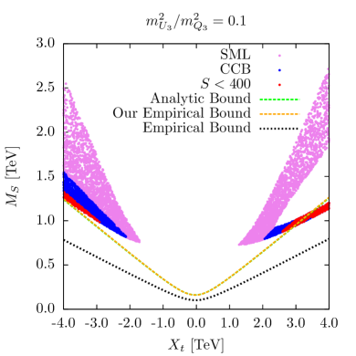
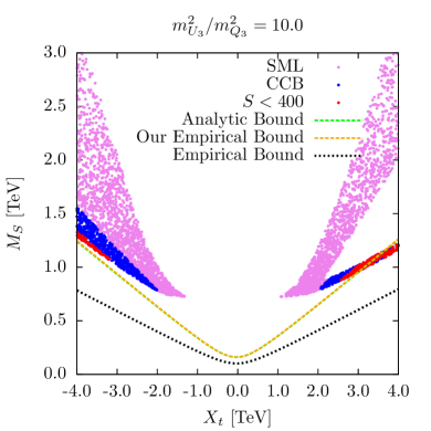
Figure 5: The deterioration of the empirical bound of Eq. (35) for $m_{U_{3}}^{2}/m_{Q_{3}}^{2}\gg 1$ or $m_{U_{3}}^{2}/m_{Q_{3}}^{2}\ll 1$. For these parameter ranges the assumption of $SU(3)_{C}$ $D$-flatness that motivated Eq. (35) breaks down and it cannot be used to reliably model the boundary between the metastable and unstable parameter regions.

We use estimate the parameters $\alpha$ and $\gamma$ by using a least-squares fit to the lower boundary of the metastable region in Fig. 1, without imposing the Higgs mass constraint. This is an arbitrary choice to fit to; different choices in Tab. 1 lead to variations in $\alpha$ on the order of $15\%$ and $100\%$ in $\gamma$. The large variation in $\gamma$ is not a big problem since it is multiplied by $|m_{2}^{2}|\sim m_{Z}^{2}\ll m_{T}^{2}$. We obtain $\alpha\simeq 3.4$ and $\gamma\simeq 60$. With $\alpha$ and $\gamma$ fixed, we fit $\beta$ to models with $r\neq 1$. We again see that there is a significant variation $\mathcal{O}(20\%)$ depending on what $r$ is, indicating that the functional form of Eq. (35) is an oversimplification. With this in mind, we find an average value of $\beta\simeq 0.5$ for $r\in[0.3,3]$. We show the resulting bound in the results of Section 3.3. For $r\simeq 1$, Eq. (35) approximates the true boundary between metastable and unstable models well. However, we expect this constraint to deteriorate as one moves away from the assumption of $SU(3)_{C}$ $D$-flatness by choosing soft masses with $r\gg 1$ or $r\ll 1$. We show an explicit example of this in Fig. 5.

We emphasize that this bound is a very rough guideline for metastability in the MSSM in a specific corner of the parameter space and should only be used as a first order approximation. A full numerical analysis is required when any of the above assumptions are violated or better precision is required.

References

- (1) S. P. Martin, In *Kane, G.L. (ed.): Perspectives on supersymmetry II* 1-153 [hep-ph/9709356].
- (2) R. Barbieri and G. F. Giudice, Nucl. Phys. B 306, 63 (1988).
- (3) C. Wymant, Phys. Rev. D 86, 115023 (2012) [arXiv:1208.1737 [hep-ph]].
- (4) G. Aad et al. [ATLAS Collaboration], Phys. Lett. B 716, 1 (2012) [arXiv:1207.7214 [hep-ex]].
- (5) S. Chatrchyan et al. [CMS Collaboration], Phys. Lett. B 716, 30 (2012) [arXiv:1207.7235 [hep-ex]].
- (6) L. J. Hall, D. Pinner and J. T. Ruderman, JHEP 1204, 131 (2012) [arXiv:1112.2703 [hep-ph]].
- (7) J. -J. Cao, Z. -X. Heng, J. M. Yang, Y. -M. Zhang and J. -Y. Zhu, JHEP 1203, 086 (2012) [arXiv:1202.5821 [hep-ph]].
- (8) J. R. Ellis, G. Ridolfi and F. Zwirner, Phys. Lett. B 257, 83 (1991).
- (9) H. E. Haber and R. Hempfling, Phys. Rev. Lett. 66, 1815 (1991).
- (10) M. S. Carena, H. E. Haber, S. Heinemeyer, W. Hollik, C. E. M. Wagner and G. Weiglein, Nucl. Phys. B 580, 29 (2000) [hep-ph/0001002].
- (11) P. Draper, P. Meade, M. Reece and D. Shih, Phys. Rev. D 85, 095007 (2012) [arXiv:1112.3068 [hep-ph]].
- (12) J. A. Casas, J. R. Espinosa, M. Quiros and A. Riotto, Nucl. Phys. B 436, 3 (1995) [Erratum-ibid. B 439, 466 (1995)] [hep-ph/9407389].
- (13) R. Kitano and Y. Nomura, Phys. Rev. D 73, 095004 (2006) [hep-ph/0602096].
- (14) J. M. Frere, D. R. T. Jones and S. Raby, Nucl. Phys. B 222, 11 (1983).
- (15) M. Claudson, L. J. Hall and I. Hinchliffe, Nucl. Phys. B 228, 501 (1983).
- (16) G. Gamberini, G. Ridolfi and F. Zwirner, Nucl. Phys. B 331, 331 (1990).
- (17) J. A. Casas, A. Lleyda and C. Munoz, Nucl. Phys. B 471, 3 (1996) [hep-ph/9507294].
- (18) T. Falk, K. A. Olive, L. Roszkowski and M. Srednicki, Phys. Lett. B 367, 183 (1996) [hep-ph/9510308].
- (19) A. Riotto and E. Roulet, Phys. Lett. B 377, 60 (1996) [hep-ph/9512401].
- (20) A. Kusenko, P. Langacker and G. Segre, Phys. Rev. D 54, 5824 (1996) [hep-ph/9602414].
- (21) J. A. Casas, A. Lleyda and C. Munoz, Phys. Lett. B 389, 305 (1996) [hep-ph/9606212].
- (22) C. Le Mouel, Nucl. Phys. B 607, 38 (2001) [hep-ph/0101351].
- (23) C. Le Mouel, Phys. Rev. D 64, 075009 (2001) [hep-ph/0103341].
- (24) M. S. Carena, M. Quiros and C. E. M. Wagner, Phys. Lett. B 380, 81 (1996) [hep-ph/9603420].
- (25) J. M. Cline, G. D. Moore and G. Servant, Phys. Rev. D 60, 105035 (1999) [hep-ph/9902220].
- (26) H. H. Patel, M. J. Ramsey-Musolf and M. B. Wise, Phys. Rev. D 88, 015003 (2013) [arXiv:1303.1140 [hep-ph]].
- (27) B. M. Kastening, Phys. Lett. B 283, 287 (1992).
- (28) C. Ford, D. R. T. Jones, P. W. Stephenson and M. B. Einhorn, Nucl. Phys. B 395, 17 (1993) [hep-lat/9210033].
- (29) R. Jackiw, Phys. Rev. D 9, 1686 (1974).
- (30) H. H. Patel and M. J. Ramsey-Musolf, JHEP 1107, 029 (2011) [arXiv:1101.4665 [hep-ph]].
- (31) N. K. Nielsen, Nucl. Phys. B 101, 173 (1975).
- (32) R. Fukuda and T. Kugo, Phys. Rev. D 13, 3469 (1976).
- (33) M. Garny and T. Konstandin, JHEP 1207, 189 (2012) [arXiv:1205.3392 [hep-ph]].
- (34) D. Metaxas and E. J. Weinberg, Phys. Rev. D 53, 836 (1996) [hep-ph/9507381].
- (35) F. James and M. Roos, Comput. Phys. Commun. 10, 343 (1975). http://lcgapp.cern.ch/project/cls/work-packages/mathlibs/minuit/index.html
- (36) S. R. Coleman, Phys. Rev. D 15, 2929 (1977) [Erratum-ibid. D 16, 1248 (1977)].
- (37) C. G. Callan, Jr. and S. R. Coleman, Phys. Rev. D 16, 1762 (1977).
- (38) G. V. Dunne and H. Min, Phys. Rev. D 72, 125004 (2005) [hep-th/0511156].
- (39) H. Min, J. Phys. A 39, 6551 (2006).
- (40) E. J. Weinberg, Phys. Rev. D 47, 4614 (1993) [hep-ph/9211314].
- (41) A. Kusenko, Phys. Lett. B 358, 51 (1995) [hep-ph/9504418].
- (42) T. Konstandin and S. J. Huber, JCAP 0606, 021 (2006) [hep-ph/0603081].
- (43) J. -h. Park, JCAP 1102, 023 (2011) [arXiv:1011.4936 [hep-ph]].
- (44) C. L. Wainwright, Comput. Phys. Commun. 183, 2006 (2012) [arXiv:1109.4189 [hep-ph]].
- (45) J. E. Camargo-Molina, B. O’Leary, W. Porod and F. Staub, Eur. Phys. J. C73, 2588 (2013) [arXiv:1307.1477 [hep-ph]].
- (46) M. Reece, New J. Phys. 15, 043003 (2013) [arXiv:1208.1765 [hep-ph]].
- (47) S. Heinemeyer, W. Hollik and G. Weiglein, Comput. Phys. Commun. 124, 76 (2000) [hep-ph/9812320].
- (48) A. Djouadi, J. -L. Kneur and G. Moultaka, Comput. Phys. Commun. 176, 426 (2007) [hep-ph/0211331].
- (49) J. Beringer et al. [Particle Data Group Collaboration], Phys. Rev. D 86, 010001 (2012).
- (50) V. Barger, P. Huang, M. Ishida and W. -Y. Keung, Phys. Lett. B 718, 1024 (2013) [arXiv:1206.1777 [hep-ph]].
- (51) S. Heinemeyer, O. Stal and G. Weiglein, Phys. Lett. B 710, 201 (2012) [arXiv:1112.3026 [hep-ph]].
- (52) J. R. Espinosa, C. Grojean, V. Sanz and M. Trott, JHEP 1212, 077 (2012) [arXiv:1207.7355 [hep-ph]].
- (53) M. Drees and K. Hagiwara, Phys. Rev. D 42, 1709 (1990).
- (54) S. Heinemeyer, W. Hollik and G. Weiglein, Phys. Rept. 425, 265 (2006) [hep-ph/0412214].
- (55) G. D’Ambrosio, G. F. Giudice, G. Isidori and A. Strumia, Nucl. Phys. B 645, 155 (2002) [hep-ph/0207036].
- (56) M. Ciuchini, G. Degrassi, P. Gambino and G. F. Giudice, Nucl. Phys. B 534, 3 (1998) [hep-ph/9806308].
- (57) B. Grzadkowski and M. Misiak, Phys. Rev. D 78, 077501 (2008) [Erratum-ibid. D 84, 059903 (2011)] [arXiv:0802.1413 [hep-ph]].
- (58) Y. Amhis et al. [Heavy Flavor Averaging Group Collaboration], arXiv:1207.1158 [hep-ex].
- (59) A. Arbey and F. Mahmoudi, Comput. Phys. Commun. 181, 1277 (2010) [arXiv:0906.0369 [hep-ph]].
- (60) G. Aad et al. [ATLAS Collaboration], arXiv:1308.2631 [hep-ex].
- (61) [ATLAS Collaboration], ATLAS-CONF-2013-068.
- (62) S. Chatrchyan et al. [CMS Collaboration], arXiv:1308.1586 [hep-ex].
- (63) [CMS Collaboration], CMS-PAS-SUS-13-004.
- (64) M. Carena, G. Nardini, M. Quiros and C. E. M. Wagner, JHEP 0810, 062 (2008) [arXiv:0806.4297 [hep-ph]].
- (65) J. Fan and M. Reece, arXiv:1401.7671 [hep-ph].
- (66) J. Hisano, K. Kawagoe, R. Kitano and M. M. Nojiri, Phys. Rev. D 66, 115004 (2002) [hep-ph/0204078].
- (67) K. Rolbiecki, J. Tattersall and G. Moortgat-Pick, Eur. Phys. J. C 71, 1517 (2011) [arXiv:0909.3196 [hep-ph]].
- (68) M. Blanke, D. Curtin and M. Perelstein, Phys. Rev. D 82, 035020 (2010) [arXiv:1004.5350 [hep-ph]].
- (69) M. Perelstein and M. Saelim, arXiv:1201.5839 [hep-ph].
- (70) M. Berggren, R. Keranen, H. Kluge and A. Sopczak, hep-ph/9911345.
- (71) E. Boos, H. U. Martyn, G. A. Moortgat-Pick, M. Sachwitz, A. Sherstnev and P. M. Zerwas, Eur. Phys. J. C 30, 395 (2003) [hep-ph/0303110].
- (72) G. F. Giudice and A. Kusenko, Phys. Lett. B 439, 55 (1998) [hep-ph/9805379].
- (73) P. Hernandez, N. Rius and V. Sanz, Nucl. Phys. Proc. Suppl. 95, 272 (2001).
- (74) J. M. Cornwall, A. Kusenko, L. Pearce and R. D. Peccei, Phys. Lett. B 718, 951 (2013) [arXiv:1210.6433 [hep-ph]].
- (75) L. Pearce, A. Kusenko and R. D. Peccei, arXiv:1307.6157 [hep-ph].
- (76) J. E. Camargo-Molina, B. O’Leary, W. Porod and F. Staub, arXiv:1309.7212 [hep-ph].
- (77) D. Chowdhury, R. M. Godbole, K. A. Mohan and S. K. Vempati, arXiv:1310.1932 [hep-ph].
- (78) N. Blinov and D. E. Morrissey, [arXiv:1309.7397 [hep-ph]].