Competition vs. Cooperation: A Game-Theoretic Decision Analysis for MIMO HetNets

Abstract

This paper addresses the problem of competition vs. cooperation in the downlink, between base stations (BSs), of a multiple input multiple output (MIMO) interference, heterogeneous wireless network (HetNet). This research presents a scenario where a macrocell base station (MBS) and a cochannel femtocell base station (FBS) each simultaneously serving their own user equipment (UE), has to choose to act as individual systems or to cooperate in coordinated multipoint transmission (CoMP). The paper employes both the theories of non-cooperative and cooperative games in a unified procedure to analyze the decision making process. The BSs of the competing system are assumed to operate at the maximum expected sum rate (MESR) correlated equilibrium (CE), which is compared against the value of CoMP to establish the stability of the coalition. It is proven that there exists a threshold geographical separation, $d_{\text{th}}$, between the macrocell user equipment (MUE) and FBS, under which the region of coordination is non-empty. Theoretical results are verified through simulations.

I Introduction

Small cells are an easily deployable solution to the increasing demand for capacity. Underlay small cells improve the capacity of the network through frequency reuse and higher link gains due to shorter distances to the user equipment (UE). On the downside the unplanned deployment of small cells in the larger cell structure creates unforeseen interference conditions. Such dynamic interference situations require novel solutions [1].

Coordinated multipoint transmission (CoMP) introduces dynamic interaction between multiple cells to increase network performance and reduce interference. In our research we consider the CoMP scheme of joint transmission (JT) [2]. We begin with the hypotheses that JT must be a rational decision, which is profitable for both macro- and femto-systems, since these systems may belong to independent operators/users. In human interactions, cooperation among a group is justifiable if all the members are better off in that group than if they were in any other group structure among themselves. This rational behavior is embedded in the solution concept of core in coalition formation games.

Past research of heterogeneous networks (HetNets) of macro- femtocells, has used both non-cooperative and cooperative games. In [3] a Stackelberg game is formulated where pricing is employed to move the equilibria towards a tolerable interference level for the macrocell base station (MBS). In [4] a potential game based analysis of Nash equilibrium (NE) of power and subcarrier allocation, for a multicell interference environment is presented. In [5] power distribution over resource blocks of cognitive femtocell base stations (FBSs) is analyzed for their correlated equilibrium (CE). In [6, 7] $\epsilon$-correlated equilibrium solution is presented for underlayed femtocells to minimize interference to the macro-system. CE is the form of equilibrium used in this paper as well.

In [8, 9] coalition formation games with externalities are used to group the femtocells to mitigate collisions and reduce interference. In [10] a coalition game together with the solution concept of recursive core is used to model the cooperative interaction between macrocell user equipment (MUE) and femtocell user equipment (FUE). They conclude that forming of disjoint coalitions increases the rates of both MUE and FUE. In [11] a coalition formation game is employed to partition a dense network of femtocells to minimize interference where they introduce a polynomial time algorithm for group formation. In [12] both transferable utility (TU) and non-transferable utility (NTU) coalition formation games are used for cooperation of receivers and transmitters in an interference environment.

This paper is set apart from the above related research, since it brings together both theories of non-cooperative and coalition formation games to model femto-maro interaction in CoMP. A similar analysis but, for non-CoMP case, is presented in [13]. The terms non-cooperative and cooperative are in accordance to their use in the game theory literature whereas the terms coordination, CoMP, and JT are used synonymously.

The rest of the paper consists of the system model in Section II, game-theoretic formulation and solution in Section III, simulation results in Section IV and conclusion with summary in Section V.

II System Model

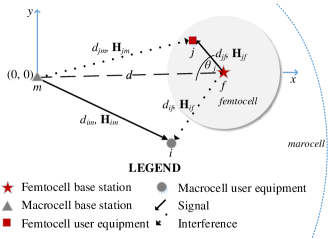
Figure 1: System model. The attributes on arrows indicate the effective distance between elements and their respective channel matrices.

The paper considers the downlink transmission of a two tier HetNet, which consists of a single MBS $m$ and a single FBS $f$, separated by a distance $d>0$. Each base station (BS) has an active user equipment (UE). It is possible that the BSs serve more than one user but the assumption is that at any given instant each BS transmits to only one selected user. The two BSs each possesses $T$ number of transmit antennas while each UE possesses $R$ number of receive antennas. Fig. 1 depicts the system model. The origin of the plane is at MBS. We define two modes of operation, namely uncoordinated and coordinated. In uncoordinated mode the two BSs act as separate transmitters where MBS serves MUE while FBS serves FUE. On the contrary if the two cells conform to the coordinated mode, then the two BSs cooperate through CoMP.

The channel model includes large scale signal attenuation as a function of distance. Channel gain matrix is multiplied by a magnitude, which is a path loss function of distance between BS and UE [14]. The received baseband equivalent signal $\mathbf{y}_{i}$ (resp. $\mathbf{y}_{j}$) at MUE $i$ (resp. FUE $j$) for uncoordinated transmission over Gaussian channel are

$$\mathbf{y}_{i} \triangleq d_{im}^{-\alpha}\mathbf{H}_{im}\mathbf{V}_{m}\mathbf{s}_{i}+d_{if}^{-\alpha}\mathbf{H}_{if}\mathbf{V}_{f}\mathbf{s}_{j}+\mathbf{n}_{i},$$ (1)

$$\mathbf{y}_{j} \triangleq d_{jf}^{-\alpha}\mathbf{H}_{jf}\mathbf{V}_{f}\mathbf{s}_{j}+d_{jm}^{-\alpha}\mathbf{H}_{jm}\mathbf{V}_{m}\mathbf{s}_{i}+\mathbf{n}_{j},$$ (2)

where $d_{im},\,d_{if},\,d_{jf},\,d_{jm}\geq 0$ are the effective distances between the respective indexed elements, $\mathbf{H}_{im}$ is the $R\times T$ complex valued channel gain matrix from MBS $m$ to MUE $i$ and $\mathbf{H}_{if},$ $\mathbf{H}_{jf},$ $\mathbf{H}_{jm}$ are interpreted analogously. The matrix $\mathbf{V}_{m}$ (resp. $\mathbf{V}_{f}$) is the precoder at MBS (resp. FBS). The independent symbol vector of unit variance at MBS $m$ (resp. at FBS $m$) to MUE $i$ (resp. to FUE $j$) is denoted by $\mathbf{s}_{i}$ (resp. $\mathbf{s}_{j}$). The exponent $\left(-\alpha\right)$, where $\alpha$ is a positive real valued scalar, accounts for path loss, and $\mathbf{n}_{i},$ $\mathbf{n}_{j}$ are circular symmetric, uncorrelated additive withe Gaussian noise (AWGN) vectors.

The achievable rate, treating interference as noise, of the macro system, $R_{\text{uc}}^{m}$, is given by (3) [15].

$$R_{\text{uc}}^{m}\triangleq\log\det\left(\mathbf{I}_{R}+\frac{d_{im}^{-2\alpha}\mathbf{H}_{im}\mathbf{V}_{m}\mathbf{V}_{m}^{H}\mathbf{H}_{im}^{H}}{d_{if}^{-2\alpha}\mathbf{H}_{if}\mathbf{V}_{f}\mathbf{V}_{f}^{H}\mathbf{H}_{if}^{H}+\sigma^{2}\mathbf{I}_{R}}\right),$$ (3)

$$R_{\text{uc}}^{f}\triangleq\log\det\left(\mathbf{I}_{R}+\frac{d_{jf}^{-2\alpha}\mathbf{H}_{jf}\mathbf{V}_{f}\mathbf{V}_{f}^{H}\mathbf{H}_{jf}^{H}}{d_{jm}^{-2\alpha}\mathbf{H}_{jm}\mathbf{V}_{m}\mathbf{V}_{m}^{H}\mathbf{H}_{jm}^{H}+\sigma^{2}\mathbf{I}_{R}}\right).$$ (4)

Above $\sigma^{2}$ is variance of circular symmetric noise and $\mathbf{I}_{R}$ is the $R\times R$ identity matrix. For a matrix $\mathbf{X}$ in the complex field, $\mathbf{X}^{H}$ denotes the Hermitian transpose. Analogously we define the achievable rate, $R_{\text{uc}}^{f}$, of the femto-system (4).

Now suppose that the two BSs coordinate through JT. The coordination is such that, FBS must transmit to both UE their respective symbols. It is possible to extend this model to include the case where both BSs transmit to both UE. The paper only consider MUE receiving JT since FUE are mostly home/office users who are less mobile and they have higher downlink gains whereas MUE may be highly mobile and operate under high signal fading and interference. The received signals at MUE and FUE in coordinated transmission are then given by (5) and (6) respectively. Note matrix augmentation in (5).

$$\mathbf{y}_{i} \triangleq d_{im}^{-\alpha}\mathbf{H}_{im}\mathbf{V}_{m}\mathbf{s}_{im}+d_{if}^{-\alpha}\mathbf{H}_{if}\mathbf{V}_{if}\mathbf{s}_{if}+\mathbf{n}_{i},$$ (5)

$$\mathbf{y}_{j} \triangleq d_{jf}^{-\alpha}\mathbf{H}_{jf}\mathbf{V}_{jf}\mathbf{s}_{j}+d_{jm}^{-\alpha}\mathbf{H}_{jm}\mathbf{V}_{m}\mathbf{s}_{im}+\mathbf{n}_{j},$$ (6)

$$R_{\text{c}}^{f} \triangleq\log\det\left(\mathbf{I}_{R}+\frac{d_{jf}^{-2\alpha}\mathbf{H}_{jf}\mathbf{V}_{jf}\mathbf{V}_{jf}^{H}\mathbf{H}_{jf}^{H}}{d_{jm}^{-2\alpha}\mathbf{H}_{jm}\mathbf{V}_{m}\mathbf{V}_{m}^{H}\mathbf{H}_{jm}^{H}+\sigma^{2}\mathbf{I}_{R}}\right).$$ (7)

Above $\mathbf{V}_{if}$ (resp. $\mathbf{V}_{jf}$) is the precoder matrix at FBS for MUE (resp. FUE), $\mathbf{V}_{m}$ is the MBS precoder. The signal model assumes that the precoders $\mathbf{V}_{if}$ and $\mathbf{V}_{jf}$ are such that there is no interuser interference from FBS to the two UE. To that end block diagonalization (BD) can be employed at FBS [16]. The independent unit variance transmission streams from MBS and FBS to MUE are $\mathbf{s}_{im}$ and $\mathbf{s}_{if}$. Then the achievable rates of FUE $R_{\text{c}}^{f}$, and MUE $R_{\text{c}}^{m}$, for the coordinated transmission scheme are given by (7) and (8) respectively [17]. This paper consider that the precoders at the two BSs are chosen from a finite predefined code-book. The finite code book model not only affords a finite action space game, but also reflects the systems in practical implementations such as LTE, which define a finite code-book.

$$R_{\text{c}}^{m}\triangleq\log\det\left(\mathbf{I}_{R}+\frac{d_{im}^{-2\alpha}}{\sigma^{2}}\mathbf{H}_{im}\mathbf{V}_{m}\mathbf{V}_{m}^{H}\mathbf{H}_{im}^{H}\right.+\left.\frac{d_{if}^{-2\alpha}}{\sigma^{2}}\mathbf{H}_{if}\mathbf{V}_{if}\mathbf{V}_{if}^{H}\mathbf{H}_{if}^{H}\right),$$ (8)

$$0\prec\mathbf{I}_{R}+d_{im}^{\prime-2\alpha}\left(d_{if}^{-2\alpha}\mathbf{B}+\mathbf{C}\right)^{\frac{-1}{2}}\mathbf{A}\left(d_{if}^{-2\alpha}\mathbf{B}+\mathbf{C}\right)^{\frac{-1}{2}}\preceq\mathbf{I}_{R}+d_{im}^{-2\alpha}\left(d_{if}^{-2\alpha}\mathbf{B}+\mathbf{C}\right)^{\frac{-1}{2}}\mathbf{A}\left(d_{if}^{-2\alpha}\mathbf{B}+\mathbf{C}\right)^{\frac{-1}{2}},$$ (9)

$$0\prec\mathbf{I}_{R}+d_{im}^{-2\alpha}\mathbf{A}^{\frac{1}{2}}\left(d_{if}^{-2\alpha}\mathbf{B}+\mathbf{C}\right)^{-1}\mathbf{A}^{\frac{1}{2}}\preceq\mathbf{I}_{R}+d_{im}^{-2\alpha}\mathbf{A}^{\frac{1}{2}}\left(d_{if}^{\prime-2\alpha}\mathbf{B}+\mathbf{C}\right)^{-1}\mathbf{A}^{\frac{1}{2}}.$$ (10)

III Core Solution

Now the paper presents two non-cooperative games one for the uncoordinated system, $\mathtt{G}_{1}$ and one for the coordinated system, $\mathtt{G}_{2}$. The relation between $\mathtt{G}_{1}$ and $\mathtt{G}_{2}$ is established in the ensuing development. Both games have identical set of players $\mathcal{\mathcal{N}\triangleq\left\{\text{MBS, FBS}\right\}}$, i.e., the two BSs. The action spaces of the players are their precoder code-books. In the uncoordinated case (resp. coordinated case) the sets of precoders of MBS and FBS are denoted by $\mathcal{A}_{m\text{uc}}$ and $\mathcal{A}_{f\text{uc}}$ (resp. $\mathcal{A}_{m\text{c}}$ and $\mathcal{A}_{f\text{c}}$) respectively. Let $\mathbf{0}\notin\mathcal{A}_{f\text{c}}$ (does not contain zero precoder), which avoids the trivial case of non-JT. The product sets of the action spaces are $\mathcal{A}_{\text{uc}}\triangleq\mathcal{A}_{m\text{uc}}\times\mathcal{A}_{f\text{uc}}$ and $\mathcal{A}_{\text{c}}\triangleq\mathcal{A}_{m\text{c}}\times\mathcal{A}_{f\text{c}}$. The utility functions of the two players in the uncoordinated case (resp. coordinated case) are $R_{\text{uc}}^{m}$ and $R_{\text{uc}}^{f}$ (resp. $R_{\text{c}}^{m}$ and $R_{\text{c}}^{f}$). The joint action of $\mathtt{G}_{1}$ is $\mathbf{V}\triangleq\left(\mathbf{V}_{m},\mathbf{V}_{f}\right)\in\mathcal{A}_{\text{uc}}$ where $\mathbf{V}_{m}\in\mathcal{A}_{m\text{uc}}$ and $\mathbf{V}_{f}\in\mathcal{A}_{f\text{uc}}$ and the joint action of $\mathtt{G}_{2}$ is $\mathbf{V}\in\mathcal{A}_{\text{c}}$ such that $\mathbf{V}\triangleq\left(\mathbf{V}_{m},\mathbf{V}_{f}\right)$ where $\mathbf{V}_{m}\in\mathcal{A}_{m\text{c}}$ and $\mathbf{V}_{f}\in\mathcal{A}_{f\text{c}}$. Note that FBS’s action $\mathbf{V}_{f}\in\mathcal{A}_{f\text{c}}$, consists of two precoders $\mathbf{V}_{f}\triangleq\left(\mathbf{V}_{if},\mathbf{V}_{jf}\right)$. The MBS (resp. FBS) has identical maximum transmit power in both uncoordinated and coordinated cases, i.e., for FBS, $\underset{\mathbf{V}\in\mathcal{A}_{f\text{uc}}}{\text{max }}\left\{\text{Trace}\left(\mathbf{V}^{H}\mathbf{V}\right)\right\}=$$\underset{\mathbf{V}_{f}\in\mathcal{A}_{f\text{c}}}{\text{max }}\left\{\text{Trace}\left(\mathbf{V}_{if}\mathbf{V}_{if}^{H}\right)+\right.\allowbreak\left.\text{Trace}\left(\mathbf{V}_{jf}\mathbf{V}_{jf}^{H}\right)\right\}$ and analogously for MBS.

Now one possesses all the ingredients necessary to define the non-cooperative games, $\mathtt{G}_{1}$ and $\mathtt{G}_{2}$. The uncoordinated game is give by the tuple $\mathtt{G}_{1}\triangleq\left\langle\mathcal{N},\mathcal{A}_{\text{uc}},\left\{R_{\text{uc}}^{m},R_{\text{uc}}^{f}\right\}\right\rangle$. The game when the two systems are in coordination is $\mathtt{G}_{2}\triangleq\left\langle\mathcal{N},\mathcal{A}_{\text{c}},\left\{R_{\text{c}}^{m},R_{\text{c}}^{f}\right\}\right\rangle$.

Let us set aside the above defined two games for a moment, we come back to them shortly. To analyze the coordinated system one must utilize coalitional games from the cooperative game theory. The most widely used solution concept in coalitional games is the core. In order for the two BSs to coordinate the core of the coalition game must be nonempty. A nonempty core implies that the grand coalition, which includes all the players, has a value, which is divisible among the players so that no other partition of subsets of players can give a better value to any of the players. The analysis of the core requires that the cooperative game has TU, which means that the sum utility of the coalition (the two cells in this case) renders itself to be shared between the members. But one observes, from the system model, that the sum rate of the coordinated system is not arbitrarily transferable between the two players. Therefore we follow a usual trick employed in such situations, introduce a monitory transfer i.e., payment, between the macro and femto systems. It is imperative to understand that such a monitory transfer is not merely a tool to make the problem amenable to coalitional game analysis, but also has an important engineering and economic aspect: coordination between the systems require sharing power with external users and communication of symbol information and channel state information (CSI) between the BSs. Such transactions have to be compensated in any practical system in order to provide an incentive to take part in CoMP. After introducing the payment $c$, the utility of MBS, $U_{\text{c}}^{m}$, and FBS, $U_{\text{c}}^{f}$, is given by (11). The payment is of units of rate, which can be interpreted in monitory terms as applicable.

$$U_{\text{c}}^{m}\triangleq R_{\text{c}}^{m}-c,\qquad U_{\text{c}}^{f}\triangleq R_{\text{c}}^{f}+c.$$ (11)

A coalitional game in characteristic form requires a set of players and a value function [18]. In this paper the set of players is $\mathcal{\mathcal{N}}$, which has three nonempty subsets.

To define the value function we revisit the games $\mathtt{G}_{1}$ and $\mathtt{G}_{2}$. There are multiple definitions of equilibria for non-cooperative games. This research is interested in CE, which is a generalization of NE [18].

Definition 1.

CE of the game $\mathtt{G}_{1}$ is a probability distribution $\tilde{p}_{\text{uc}}\left(\cdot\right)$ on the joint action space $\mathcal{A}_{\text{uc}}$ such that $\forall$ $\mathbf{V}\in\mathcal{A}_{\text{uc}}$, $\forall$ $\mathbf{V}_{m}^{\prime}\in\mathcal{A}_{m\text{uc}}$, and $\forall$ $\mathbf{V}_{f}^{\prime}\in\mathcal{A}_{f\text{uc}}$

$$\sum_{\mathbf{V}:\mathbf{V}_{f}\in\mathcal{A}_{f\text{uc}}}\tilde{p}_{\text{uc}}\left(\mathbf{V}\right)R_{\text{uc}}^{m}\left(\mathbf{V}\right)\geq \sum_{\mathbf{V}:\mathbf{V}_{f}\in\mathcal{A}_{f\text{uc}}}\tilde{p}_{\text{uc}}\left(\mathbf{V}\right)R_{\text{uc}}^{m}\left(\mathbf{V}_{m}^{\prime},\mathbf{V}_{f}\right),$$ (12)

$$\sum_{\mathbf{V}:\mathbf{V}_{m}\in\mathcal{A}_{m\text{uc}}}\tilde{p}_{\text{uc}}\left(\mathbf{V}\right)R_{\text{uc}}^{f}\left(\mathbf{V}\right)\geq \sum_{\mathbf{V}:\mathbf{V}_{m}\in\mathcal{A}_{m\text{uc}}}\tilde{p}_{\text{uc}}\left(\mathbf{V}\right)R_{\text{uc}}^{f}\left(\mathbf{V}_{f}^{\prime},\mathbf{V}_{m}\right).$$ (13)

Similarly we define the CE of the game $\mathtt{G}_{2}$, the probability distribution $\tilde{p}_{\text{c}}\left(\cdot\right)$ on the action space $\mathcal{A}_{\text{c}}$, which satisfies $\forall$ $\mathbf{V}\in\mathcal{A}_{\text{c}}$, $\forall\,\mathbf{V}_{m}^{\prime}\in\mathcal{A}_{m\text{c}}$, and $\forall\,\mathbf{V}_{f}^{\prime}\in\mathcal{A}_{f\text{c}}$

$$\sum_{\mathbf{V}:\mathbf{V}_{f}\in\mathcal{A}_{f\text{c}}}\tilde{p}_{\text{c}}\left(\mathbf{V}\right)R_{\text{c}}^{m}\left(\mathbf{V}\right) \geq\sum_{\mathbf{V}:\mathbf{V}_{f}\in\mathcal{A}_{f\text{c}}}\tilde{p}_{\text{c}}\left(\mathbf{V}\right)R_{\text{c}}^{m}\left(\mathbf{V}_{m}^{\prime},\mathbf{V}_{f}\right),$$ (14)

$$\sum_{\mathbf{V}:\mathbf{V}_{m}\in\mathcal{A}_{m\text{c}}}\tilde{p}_{\text{c}}\left(\mathbf{V}\right)R_{\text{c}}^{f}\left(\mathbf{V}\right) \geq\sum_{\mathbf{V}:\mathbf{V}_{m}\in\mathcal{A}_{m\text{c}}}\tilde{p}_{\text{c}}\left(\mathbf{V}\right)R_{\text{c}}^{f}\left(\mathbf{V}_{f}^{\prime},\mathbf{V}_{m}\right).$$ (15)

While a finite game is guaranteed to have at least one CE, in most cases there are an infinite set of CE [18]. Out of this set of CE this paper choose the equilibrium, which maximizes the expected sum rate. The maximum expected sum rate correlated equilibrium (MESR-CE) of game $\mathtt{G}_{1}$ is the probability distribution obtained through solving the following linear system;

$$\underset{\mathbf{p}_{\text{uc}}}{\text{maximize }} \sum_{\mathbf{V}\in\mathcal{\mathcal{A}_{\text{uc}}}}p_{\text{uc}}\left(\mathbf{V}\right)\left(R_{\text{uc}}^{m}\left(\mathbf{V}\right)+R_{\text{uc}}^{f}\left(\mathbf{V}\right)\right),$$

subject to $$\left(\ref{eq:CEg1m}\right),\,\left(\ref{eq:CEg1f}\right),$$ (16)

$$\sum_{\mathbf{\mathbf{V}}\in\mathcal{\mathcal{A}_{\text{uc}}}}p_{\text{uc}}\left(\mathbf{V}\right)=1,$$

$$p_{\text{uc}}\left(\mathbf{V}\right)\geq 0,\,\forall\,\mathbf{V}\in\mathcal{\mathcal{A}_{\text{uc}}},$$

where $p_{\text{uc}}\left(\mathbf{V}\right)$ is the probability of joint action $\mathbf{V}\in\mathcal{\mathcal{A}_{\text{uc}}}$ and $\mathbf{p}_{\text{uc}}\triangleq\left(p_{\text{uc}}\left(\mathbf{V}\right)\right)_{\mathbf{v}\in\mathcal{\mathcal{A}_{\text{uc}}}}$. The expected rate of each player at CE of $\mathtt{G}_{1}$ is

$$R_{\text{uc,cor}}^{m} \triangleq \sum_{\mathbf{V}\in\mathcal{\mathcal{A}_{\text{uc}}}}\tilde{p}_{\text{uc}}\left(\mathbf{V}\right)R_{\text{uc}}^{m}\left(\mathbf{V}\right),$$ (17)

$$R_{\text{uc,cor}}^{f} \triangleq \sum_{\mathbf{V}\in\mathcal{\mathcal{A}_{\text{uc}}}}\tilde{p}_{\text{uc}}\left(\mathbf{V}\right)R_{\text{uc}}^{f}\left(\mathbf{V}\right),$$ (18)

where $\tilde{p}_{\text{uc}}\left(\cdot\right)$ is the MESR-CE solution of the linear program (16).

Analogously one can obtain the MESR-CE of game $\mathtt{G}_{2}$ as the solution to the following linear system;

$$R_{\text{c, cor}}\triangleq\underset{\mathbf{p}_{\text{c}}}{\text{maximize }} \sum_{\mathbf{V}\in\mathcal{A}_{\text{c}}}p_{\text{c}}\left(\mathbf{V}\right)\left(R_{\text{c}}^{m}\left(\mathbf{V}\right)+R_{\text{c}}^{f}\left(\mathbf{V}\right)\right),$$

subject to $$\left(\ref{eq:CEg2m}\right),\,\left(\ref{eq:CEg2f}\right),$$ (19)

$$\sum_{\mathbf{V}\in\mathcal{A}_{\text{c}}}p_{\text{c}}\left(\mathbf{V}\right)=1,$$

$$p_{\text{c}}\left(\mathbf{V}\right)\geq 0,\,\forall\,\mathbf{V}\in\mathcal{A}_{\text{c}},$$

where $\mathbf{p}_{\text{c}}\triangleq\left(p_{\text{c}}\left(\mathbf{V}\right)\right)_{\mathbf{V}\in\mathcal{\mathcal{A}_{\text{c}}}}$. Let $\tilde{p}_{\text{c}}\left(\cdot\right)$ be the MESR-CE distribution of game $\mathtt{G}_{2}$. The expected rate of each player at CE of $\mathtt{G}_{2}$ is

$$R_{\text{c,cor}}^{m} \triangleq \sum_{\mathbf{V}\in\mathcal{\mathcal{A}_{\text{c}}}}\tilde{p}_{\text{c}}\left(\mathbf{V}\right)R_{\text{c}}^{m}\left(\mathbf{V}\right),$$ (20)

$$R_{\text{c,cor}}^{f} \triangleq \sum_{\mathbf{V}\in\mathcal{\mathcal{A}_{\text{c}}}}\tilde{p}_{\text{c}}\left(\mathbf{V}\right)R_{\text{c}}^{f}\left(\mathbf{V}\right).$$ (21)

Now the value function $v\left(\cdot\right)$ of the coalition game is as follows;

$$v\left(\mathcal{S}\right)\triangleq\begin{cases}R_{\text{uc,cor}}^{m}&\mathcal{S}=\left\{\text{MBS}\right\},\\ R_{\text{uc, cor}}^{f}&\mathcal{S}=\left\{\text{FBS}\right\},\\ R_{\text{c, cor}}&\mathcal{S}=\mathcal{N}.\end{cases}$$ (22)

At this point let us recap the development of this section so far: in the above definition of the value function $v\left(\mathcal{S}\right)$, $R_{\text{uc,cor}}^{m}$ in (17) (resp. $R_{\text{uc, cor}}^{f}$ in (18)) is the expected rate obtained by the macro system (resp. femto system) while playing the MESR-CE in $\mathtt{G}_{1}$. On the other hand the value of the grand coalition, $R_{\text{c, cor}}$ in (19), is the MESR of the two BSs while playing the MESR-CE in $\mathtt{G}_{2}$. Then the coalitional game in characteristic form is defined by the tuple $\mathtt{G}_{3}\triangleq\left\langle\mathcal{N},v\left(\cdot\right)\right\rangle$.

Definition 2.

The core is the set of allocations such that no subgroup within the coalition can do better by leaving to form other coalitions [18].

In our game the set of allocations are $U_{\text{c}}^{m}$ and $U_{\text{c}}^{f}$ in (11), such that $U_{\text{c}}^{m}+U_{\text{c}}^{f}=R_{\text{c, cor}}$.

III-A Region of Coordination

As MUE moves closer to FBS, signal level drops and interference level rises, hence one expects cooperation with FBS to be preferable to MBS. Since the sum rate can be apportioned between the two systems through the monitory transfer, one expects to find a $c$, at which the core is non empty. The region where the core is non empty is called, the region of coordination or identically CoMP region. In a single input single output (SISO) system a signal to interference plus noise ratio (SINR) based argument easily demonstrates the existence of a core but the argument for MIMO requires a bit more analysis.

Proposition 1.

$v\left(\mathcal{N}\right)\geq v\left(\text{MBS}\right)+v\left(\text{FBS}\right)$ if and only if there exists a payment $c$ such that $U_{\text{c}}^{m}\geq R_{\text{uc,cor}}^{m}$ and $U_{\text{c}}^{f}\geq R_{\text{uc,cor}}^{f}$.

Proof:

We provide a constructive proof. By (11) and while $\mathtt{G}_{2}$ system is in CE the utilities are $U_{\text{c}}^{m}=R_{\text{c,cor}}^{m}-c$ and $U_{\text{c}}^{f}=R_{\text{c,cor}}^{m}+c$. Let us consider the LHS of iff, which is equivalent to $R_{\text{c, cor}}\geq R_{\text{uc,cor}}^{m}+R_{\text{uc,cor}}^{f}$, which implies either $R_{\text{c,cor}}^{m}\geq R_{\text{uc,cor}}^{m}$ or $R_{\text{c,cor}}^{f}\geq R_{\text{uc,cor}}^{f}$ or both. Let us take the case where $R_{\text{c,cor}}^{m}\geq R_{\text{uc,cor}}^{m}$ and $R_{\text{c,cor}}^{f}\leq R_{\text{uc,cor}}^{f}$, all other cases can be similarly proven. Then there exists a positive constant $c$ such that $\left(R_{\text{c,cor}}^{m}-c\right)=U_{\text{c}}^{m}\geq R_{\text{uc,cor}}^{m}$ and $\left(R_{\text{c,cor}}^{f}+c\right)=U_{\text{c}}^{f}\geq R_{\text{uc,cor}}^{f}$ since $\left(R_{\text{c,cor}}^{m}-c\right)+\left(R_{\text{c,cor}}^{f}+c\right)\geq\allowbreak R_{\text{uc,cor}}^{m}+R_{\text{uc,cor}}^{f}$. Converse (RHS$\implies$LHS) is proven simply by summing the two inequalities $U_{\text{c}}^{m}\geq R_{\text{uc,cor}}^{m}$ and $U_{\text{c}}^{f}\geq R_{\text{uc,cor}}^{f}$. ∎

Proposition 1 claims that $R_{\text{c, cor}}\geq R_{\text{uc,cor}}^{m}+R_{\text{uc,cor}}^{m}$ is a necessary and sufficient condition for the core of $\mathtt{G}_{3}$ to be nonempty.

In order to establish the final result we need the following propositions.

Proposition 2.

$R_{\text{uc}}^{m}$ is monotonically decreasing in $d_{im}$ and monotonically increasing in $d_{if}$.

Proof:

The proof depends on Loewner ordering of positive semidefinite (PSD) matrices ([19] 7.7). For two PSD matrices $\mathbf{A}$, $\mathbf{B}$, we write $\mathbf{A}\succeq\mathbf{B}$ (resp. $\mathbf{A}\succ\mathbf{B}$) if $\mathbf{A}-\mathbf{B}\succeq 0$ is PSD (resp. $\mathbf{A}-\mathbf{B}\succ 0$ positive definite (PD)). Let $\mathbf{A}\triangleq\mathbf{H}_{im}\mathbf{V}_{m}\mathbf{V}_{m}^{H}\mathbf{H}_{im}^{H}$, $\mathbf{B}\triangleq\mathbf{H}_{if}\mathbf{V}_{f}\mathbf{V}_{f}^{H}\mathbf{H}_{if}^{H}$ and $\mathbf{C}\triangleq\sigma^{2}\mathbf{I}_{R}$. $\mathbf{A},\mathbf{B}$ are PSD and $\mathbf{C}$ is PD, also $d_{if}^{-2\alpha}\mathbf{B}+\mathbf{C}$ is PD. Then the capacity of maro-system (3) can be reformulated as

$$R_{\text{uc}}^{m}=\log\det\left(\mathbf{I}_{R}+d_{im}^{-2\alpha}\left(d_{if}^{-2\alpha}\mathbf{B}+\mathbf{C}\right)^{-\frac{1}{2}}\mathbf{A}\left(d_{if}^{-2\alpha}\mathbf{B}+\mathbf{C}\right)^{\frac{-1}{2}}\right).$$

Let $0<d_{im}<d_{im}^{\prime}$, so (9) (see page above) holds, therefore the determinant of (24) is no less than the determinant of (23), which implies that the determinant is monotonically decreasing in $d_{im}$.

$$\mathbf{I}_{R}+d_{im}^{\prime-2\alpha}\left(d_{if}^{-2\alpha}\mathbf{B}+\mathbf{C}\right)^{\frac{-1}{2}}\mathbf{A}\left(d_{if}^{-2\alpha}\mathbf{B}+\mathbf{C}\right)^{\frac{-1}{2}}.$$ (23)

$$\mathbf{I}_{R}+d_{im}^{-2\alpha}\left(d_{if}^{-2\alpha}\mathbf{B}+\mathbf{C}\right)^{\frac{-1}{2}}\mathbf{A}\left(d_{if}^{-2\alpha}\mathbf{B}+\mathbf{C}\right)^{\frac{-1}{2}}.$$ (24)

Next we reformulate (3),

$$R_{\text{uc}}^{m}=\log\det\left(\mathbf{I}_{R}+d_{im}^{-2\alpha}\mathbf{A}^{\frac{1}{2}}\left(d_{if}^{-2\alpha}\mathbf{B}+\mathbf{C}\right)^{-1}\mathbf{A}^{\frac{1}{2}}\right),$$

and let $0<d_{if}<d_{if}^{\prime}$. Then (10) holds and by a similar argument to above we have that the determinant is increasing in $d_{if}$. This completes the proof. ∎

Now we consider the properties of $R_{\text{c}}^{m}.$

Proposition 3.

$R_{\text{c}}^{m}\left(\cdot\right)$ is monotonically increasing in $d_{if}^{-2\alpha}$ and $d_{im}^{-2\alpha}$ and is bounded from below by

$$\gamma^{m}\left(d_{if},\mathbf{V}_{if}\right)\triangleq\log\det\left(\mathbf{I}_{R}+\frac{1}{\sigma^{2}}d_{if}^{-\alpha}\mathbf{H}_{if}\mathbf{V}_{if}\mathbf{V}_{if}^{H}d_{if}^{-\alpha}\mathbf{H}_{if}^{H}\right).$$

Proof:

The proof utilizes Weyl’s inequality for Hermitian matrices [20]. Let us first consider $d_{if}^{-2\alpha}$.Suppose $\mathbf{X},$ $\mathbf{Y}$ are two Hermitian matrices of size $n\times n$, then the Weyl’s inequality states that

$$\lambda_{i}(\mathbf{X})+\lambda_{n}(\mathbf{Y})\leq\lambda_{i}(\mathbf{X}+\mathbf{Y})\leq\lambda_{i}(\mathbf{X})+\lambda_{1}(\mathbf{Y}),\quad i=1,\ldots,n,$$

where $\lambda_{i}(\mathbf{X})$ is the $i^{\mathrm{th}}$ largest eigenvalue of $\mathbf{X}$, i.e., largest eigenvalue is $\lambda_{1}\left(\mathbf{X}\right)$ and smallest is $\lambda_{n}\left(\mathbf{X}\right)$. If $\mathbf{X}$, $\mathbf{Y}$ are positive semidefinite (PSD) note that the inequality reduces to

$$0\leq\lambda_{i}(\mathbf{X})\leq\lambda_{i}(\mathbf{X}+\mathbf{Y})\leq\lambda_{i}(\mathbf{X})+\lambda_{1}(\mathbf{Y}),\quad i=1,\ldots,n.$$

Let $\mathbf{X}=\mathbf{I}_{R}+\frac{d_{im}^{-2\alpha}}{\sigma^{2}}\mathbf{H}_{im}\mathbf{V}_{m}\mathbf{V}_{m}^{H}\mathbf{H}_{im}^{H}+\frac{d_{if}^{-2\alpha}}{\sigma^{2}}\mathbf{H}_{if}\mathbf{V}_{if}\mathbf{V}_{if}^{H}\mathbf{H}_{if}^{H}$ and $\mathbf{Y}=\frac{\delta}{\sigma^{2}}\mathbf{H}_{if}\mathbf{V}_{if}\mathbf{V}_{if}^{H}\mathbf{H}_{if}^{H}$ where $\delta\in\mathbb{R}_{+}$. Then monotonicity in $d_{if}^{-2\alpha}$ follows from

$$0<\det\left(\mathbf{X}\right)=\prod_{i}\lambda_{i}(\mathbf{X})\leq\det\left(\mathbf{X}+\mathbf{Y}\right)=\prod_{i}\lambda_{i}(\mathbf{X}+\mathbf{Y}).$$

Similarly the proof extends to $d_{im}^{-2\alpha}$. Then setting $d_{im}^{-2\alpha}=0$ the lower bound is achieved. ∎

Theorem 1.

For some $d>0$ under Assumption 1, $\exists$ $d_{\text{th}}$ such that for $d_{if}\leq d_{\text{th}}$, the region of cooperation is nonempty.

Proof:

Let $\mathbf{V}=\left(\mathbf{V}_{if},\mathbf{V}_{jf}\right)\in\mathcal{A}_{\text{c}}$, $\mathbf{V}^{\prime}\in\mathcal{A}_{\text{uc}}$ be any two actions from the respective spaces and let the location of the FUE be fixed relative to the FBS at $\left(\bar{d}_{jf},\bar{\theta}_{j}\right)$. Then $R_{\text{c}}^{f}\left(\mathbf{V}\right)$ and $R_{\text{uc}}^{f}\left(\mathbf{V}^{\prime}\right)$ are constants irrespective of location of MUE. Now consider that MUE moves along a trajectory with decreasing $d_{if}$ and increasing $d_{im}$. By Proposition 2, $R_{\text{uc}}^{m}\left(\mathbf{V}^{\prime}\right)$ is decreasing. As $d_{if}\rightarrow 0$, by Proposition 3, $R_{c}^{m}\left(d_{if},\cdot\right)\rightarrow\infty$. Therefore there must exist $d_{if}\leq d_{\text{th}}$, such that $R_{c}^{m}\left(d_{if},\cdot\right)+R_{\text{c}}^{f}\left(\mathbf{V}\right)\geq\allowbreak R_{\text{uc}}^{m}\left(\mathbf{V}^{\prime}\right)+R_{\text{uc}}^{f}\left(\mathbf{V}^{\prime}\right)$. Since the action choice was arbitrary $\exists$ $d_{\text{th}}$ such that, $\underset{\mathbf{V}\in\mathcal{A}_{\text{c}}}{\text{min }}\left(R_{\text{c}}^{m}\left(\mathbf{V}\right)+R_{\text{c}}^{f}\left(\mathbf{V}\right)\right)\geq\allowbreak\underset{\mathbf{V}\in\mathcal{A}_{\text{uc}}}{\text{max }}\left(R_{\text{uc}}^{m}\left(\mathbf{V}\right)+R_{\text{uc}}^{f}\left(\mathbf{V}\right)\right).$

Therefore $\forall$ probability distributions $\tilde{p}_{\text{uc}}$ and $\tilde{p}_{\text{c}}$, we have $\sum_{\mathbf{V}\in\mathcal{A}_{\text{c}}}\tilde{p}_{\text{c}}\left(\mathbf{V}\right)\left(R_{\text{c}}^{m}\left(\mathbf{V}\right)+R_{\text{c}}^{f}\left(\mathbf{V}\right)\right)\geq\allowbreak\sum_{\mathbf{V}\in\mathcal{A}_{\text{uc}}}\tilde{p}_{\text{uc}}\left(\mathbf{V}\right)\left(R_{\text{uc}}^{m}\left(\mathbf{V}\right)+R_{\text{uc}}^{f}\left(\mathbf{V}\right)\right).$ This completes the proof. ∎

Theorem 1 together with Proposition 1 suggests the existence of a region around the FBS where the core is nonempty. Thus we establish the rationality of CoMP scheme JT.

IV Numerical Results

The distances are measured in meters (m), we locate MBS at $\left(0,0\right)$, FBS at $\left(1000,0\right)$, and FUE $\left(990,0\right)$. Unless otherwise stated, the default maximum transmit power of MBS is $5$ W and of FBS is $1$ W. The two BSs each has $4$ antennas and each UE has $2$ antennas. In the coordinated mode of transmission, by default FBS distributes the power evenly among FUE and MUE. The AWGN power is set at $10^{-4}$ W. In the Fig. 2 MUE moves from far negative $x$ region towards the FBS in linear trajectories. One such trajectory is shown in the figure. The region where coordination is preferred over uncoordinated transmission is marked. The symmetry in the region is due to the use of symmetric channel matrices on either side of the FBS.

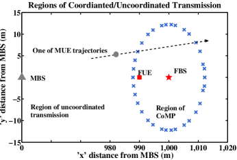
Figure 2: Region of coordination.

In the rest of the figures the trajectory of the MUE is on the $x$ axis ($y$ coordinate is $0$). Fig. 3 denotes the expansion of the CoMP region as the FBS transmit power increases. One also sees from the figure that $R_{\text{c, cor}}$ far exceeds $R_{\text{uc, cor}}$ as MUE approaches FBS. Fig. 4 shows, on the plan of $\left(x,\,y\right)$, the excess value of the coalition over the value of uncoordinated system.

Figure 3: Dependence of CoMP region on FBS transmit power.

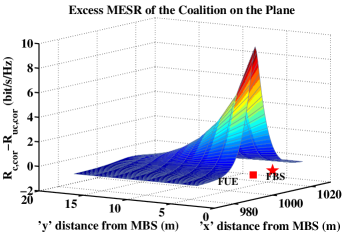
Figure 4: Geometric distribution of value of coalition, $v\left(\mathcal{N}\right),$ over uncoordinated system.

Fig. 5 demonstrates that as the amount of power allocated to MUE increases the diameter of the coordination region shrinks. The term diameter is loosely used to mean the distance between the entry point and exit point of CoMP region when the MUE’s trajectory is on $x$ axis ($y$ coordinate $0$). Consider the two MUE power ratios of $a$ and $c$ such that $c>a$. Then the explanation for the phenomenon seen in Fig. 5 is that while operating at ratio $c$ if the FBS switches to CoMP at the coordination boundary of the ratio $a$ then the reduction of FUE rate is higher than the increase in MUE rate as still MUE is further away from FBS than FUE, thus discouraging the formation of the coalition till MUE moves closer to FBS.

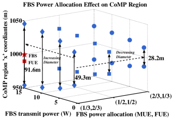
Figure 5: The variation of the diameter of the CoMP region with FBS power allocation ratio $\left(a,b\right)$. Here $\left(a,b\right)$ implies $a$ and $b$ fractions of power are assigned to MUE and FUE respectively.

V Conclusion

This paper considered the downlink of a HetNet consisting of a maro- and a femtocell. Two non-cooperative games were devised. The first game, $\mathtt{G}_{1}$, had the two cells in competition. In the second game, $\mathtt{G}_{2}$, the cells were in coordination (CoMP). In each game the cells operated in the respective maximum expected sum rate-correlated equilibria (MESR-CE). Then a third game, $\mathtt{G}_{3}$, was defined which is a coalition game in characteristic form with transferable utility. In $\mathtt{G}_{3}$ the value of the coalition was allowed to be arbitrarily transferred between the two cells via a payment. The solution mechanism of core, was used in the coalitional games $\mathtt{G}_{3}$ with value function based on MESR-CE of $\mathtt{G}_{1}$ and $\mathtt{G}_{2}$. Then the paper proved the existence of a region where the core of the game $\mathtt{G}_{3}$ is nonempty, which demonstrates that CoMP is a rational decision in some region and the CoMP decision making is reduced to identifying a threshold separation $d_{\text{th}}$. CoMP decision mechanisms for more complex channel models with more than two cells can be considered in future work.

Acknowledgment

We thank Prof. N. Rajatheva of University of Oulu, Finland and Dr. F. Poloni of University of Pisa, Italy, for their valuable insight in proofs. We also thank the StackExchange forums for providing a platform of discussion.

References

• [1] T. Zahir, K. Arshad, A. Nakata, and K. Moessner, “Interference management in femtocells,” IEEE Commun. Surveys Tuts., vol. 15, no. 1, pp. 293–311, 2013.
• [2] M. Sawahashi, Y. Kishiyama, A. Morimoto, D. Nishikawa, and M. Tanno, “Coordinated multipoint transmission/reception techniques for lte-advanced [coordinated and distributed mimo],” IEEE Wireless Commun. Mag., vol. 17, no. 3, pp. 26–34, 2010.
• [3] X. Kang, R. Zhang, and M. Motani, “Price-based resource allocation for spectrum-sharing femtocell networks: A stackelberg game approach,” IEEE J. Sel. Areas Commun., vol. 30, no. 3, pp. 538–549, 2012.
• [4] S. Buzzi, G. Colavolpe, D. Saturnino, and A. Zappone, “Potential games for energy-efficient power control and subcarrier allocation in uplink multicell ofdma systems,” IEEE J. Sel. Topics Signal Process., vol. 6, no. 2, pp. 89–103, 2012.
• [5] J. Huang and V. Krishnamurthy, “Cognitive base stations in LTE/3GPP femtocells: A correlated equilibrium game-theoretic approach,” IEEE Trans. Commun., vol. 59, no. 12, pp. 3485–3493, 2011.
• [6] M. Bennis, S. M. Perlaza, and M. Debbah, “Learning coarse correlated equilibria in two-tier wireless networks,” in Proc. IEEE International Conference on Communications (ICC), 2012, pp. 1592–1596.
• [7] W.-S. Lai, M.-E. Chiang, S.-C. Lee, and T.-S. Lee, “Game theoretic distributed dynamic resource allocation with interference avoidance in cognitive femtocell networks,” in Proc. IEEE Wireless Communications and Networking Conference (WCNC), 2013, pp. 3364–3369.
• [8] F. Pantisano, M. Bennis, W. Saad, R. Verdone, and M. Latva-aho, “Coalition formation games for femtocell interference management: A recursive core approach,” in Proc. IEEE Wireless Communications and Networking Conference (WCNC), 2011, pp. 1161–1166.
• [9] Z. Zhang, L. Song, Z. Han, W. Saad, and Z. Lu, “Overlapping coalition formation games for cooperative interference management in small cell networks,” in Proc. IEEE Wireless Communications and Networking Conference (WCNC), 2013, pp. 643–648.
• [10] F. Pantisano, M. Bennis, W. Saad, and M. Debbah, “Spectrum leasing as an incentive towards uplink macrocell and femtocell cooperation,” IEEE J. Sel. Areas Commun., vol. 30, no. 3, pp. 617–630, 2012.
• [11] B. Ma, M. Cheung, and W. V.W.S., “Interference management for multimedia femtocell networks with coalition formation game,” in Proc. IEEE International Conference on Communications (ICC), 2013, pp. 4705–4710.
• [12] S. Mathur, L. Sankar, and N. B. Mandayam, “Coalitions in cooperative wireless networks,” IEEE J. Sel. Areas Commun., vol. 26, no. 7, pp. 1104–1115, 2008.
• [13] E. Larsson and E. Jorswieck, “Competition versus cooperation on the miso interference channel,” IEEE J. Sel. Areas Commun., vol. 26, no. 7, pp. 1059–1069, 2008.
• [14] J. Zhang and J. Andrews, “Adaptive spatial intercell interference cancellation in multicell wireless networks,” IEEE J. Sel. Areas Commun., vol. 28, no. 9, pp. 1455–1468, December 2010.
• [15] S. Christensen, R. Agarwal, E. Carvalho, and J. Cioffi, “Weighted sum-rate maximization using weighted MMSE for MIMO-BC beamforming design,” IEEE Trans. Wireless Commun., vol. 7, no. 12, pp. 4792–4799, 2008.
• [16] Y. Hadisusanto, L. Thiele, and V. Jungnickel, “Distributed base station cooperation via block-diagonalization and dual-decomposition,” in Proc. IEEE Global Telecommunications Conference,(GLOBECOM ’08), Nov. 2008, pp. 1–5.
• [17] D. Tse and P. Viswanath, Fundamentals of Wireless Communication.   New York, NY, USA: Cambridge University Press, 2005.
• [18] N. Nisan, T. Roughgarden, E. Tardos, and V. V. Vazirani, Algorithmic game theory.   Cambridge University Press, 2007.
• [19] R. Horn and C. Johnson, Matrix Analysis.   Cambridge University Press, 2012.
• [20] J. Franklin, Matrix Theory, ser. Dover Books on Mathematics.   Dover Publications, 2000.