Variation in the dust emissivity index across M33 with Herschel and Spitzer (HerM33es)

We study the wavelength dependence of the dust emission as a function of position and environment across the disk of M33 at a linear resolution of 160 pc using Spitzer and Herschel photometric data. M33 is a Local Group spiral with a slightly subsolar metallicity, making it an ideal stepping-stone to less regular and lower metallicity objects such as dwarf galaxies and, probably, young universe objects. Expressing the emissivity of the dust as a power law, the power-law exponent ($\beta$) is estimated from two independent approaches designed to properly treat the degeneracy between $\beta$ and the dust temperature. Both $\beta$ and the dust temperature are higher in the inner disk than in the outer disk, contrary to reported $\beta-T$ anti-correlations found in other sources. In the cold $+$ warm dust model, the warm component and the ionized gas (H$\alpha$) have a very similar distribution across the galaxy, demonstrating that the model separates the components in an appropriate fashion. The flocculent spiral arms and the dust lanes are evident in the map of the cold component. Both cold and warm dust column densities are high in star forming regions and reach their maxima toward the giant star forming complexes NGC604 and NGC595. $\beta$ declines from close to 2 in the center to about 1.3 in the outer disk. $\beta$ is positively correlated with star formation and with molecular gas column, as traced by H$\alpha$ and CO emission. The lower dust emissivity index in the outer parts of M33 is likely related to the reduced metallicity (different grain composition) and possibly different size distribution. It is not due to the decrease in stellar radiation field or temperature in a simple way because the FIR-bright regions in the outer disk also have a low $\beta$. Like most spirals, M33 has a (decreasing) radial gradient in star formation and molecular-to-atomic gas ratio such that the regions bright in H$\alpha$ or CO tend to trace the inner disk, making it difficult to distinguish between their effects on the dust. The assumption of a constant emissivity index $\beta$ is obviously not appropriate.

1 Introduction

Dust and gas are thoroughly mixed in the interstellar medium (ISM), with approximately half of the metals (atomic number Z$>$2) in each. Unlike molecules, which radiate at specific frequencies, dust emission covers all frequencies and carries much more energy. Dust emission thus provides an alternative to spectral lines to study the mass distribution in the ISM. Dust has the advantage over the commonly-used CO molecule of not being photo-dissociated by UV photons. However, dust emission depends strongly on the grain temperature, such that it is not straightforward to measure the dust mass. In order to estimate the grain temperature or range in temperatures, it is necessary to know how grain emission varies with wavelength.

For dust grains in local thermal equilibrium, the temperature is usually obtained using a modified black body (MBB) emission given by

$$S_{\nu}=\,B_{\nu}(T)\,[1-exp(-\tau_{\nu})],$$ (1)

where $S_{\nu}$ is the intensity, $B_{\nu}$ represents the Planck function, and $\tau_{\nu}$ denotes the optical depth of the dust, depending on frequency $\nu$. In the optically thin limit, the above equation converts to

$$S_{\nu}=\,B_{\nu}(T)\,\tau_{\nu}=\,B_{\nu}(T)\,\kappa_{\nu}\,\Sigma_{\rm dust},$$ (2)

where $\Sigma_{\rm dust}$ is the dust mass surface density and $\kappa_{\nu}=\kappa_{0}\,(\nu/\nu_{0})^{\beta}$ is the dust emissivity with index $\beta$ ($\kappa_{0}$ is the grain cross-section per gram at frequency $\nu_{0}$).

There is some evidence supporting variations of the dust emission spectrum with environmental conditions from both Galactic [e.g. 48] and extra-galactic studies [e.g. 41]. The dust emissivity index $\beta$ could change depending on grain properties such as structure, size distribution, or chemical composition and is still a matter of debate. These properties may be affected by different physical/environmental processes like shattering, sputtering, grain - grain collisions [mainly due to shocks, see e.g. 33, and references therein], condensation of molecules onto grains, and coagulation [e.g. 16]. The extra-galactic observations presented here sample a beam of 160 pc with a depth of few 100 pc (Combes et al. 2012). Along each line-of-sight, we therefore expect to sample regions of widely different physical properties, e.g. temperatures and densities. The observed dust temperatures and $\beta$ indices are therefore weighted averages of the local conditions along the lines of sight. This is further discussed in Section 6. Neglecting the variation in the dust emissivity index could be misleading when determining the dust mass [e.g. 43]. For instance, from the long-wavelength COBE data [55], assuming a constant $\beta$, found a very massive cold dust component in the Milky Way (MW) but this was not confirmed by [39].

Nearby galaxies provide ideal astrophysical laboratories (1) with different chemical abundances and (2) where - for face on galaxies - the galactic disk is only crossed once by our line of sight, so it is straightforward to distinguish spiral arms, associate gas/dust clouds with star forming regions, and inter-arm regions.

The Herschel Space Observatory [49] provides far-infrared (FIR) and sub-millimeter (sub-mm) data at high angular resolution and sensitivity over the wavelengths required to investigate the physical properties of dust in galaxies. Recent studies have suggested that the emission of dust grains could differ from the standard MBB model (see Eq. 1) which assumes a $\beta$=2 emissivity law. This can lead to unphysical gas-to-dust mass ratios compared to those expected from the metallicity of the galaxies [44, 23, 24, 32]. The emissivity indices reported from observations range from $\beta=1$ to $\beta=2.5$ [10, 9, 4]. Theoretically, $\beta<1$ is excluded at the FIR and submm wavelengths, otherwise the Kramers-Kronig relation does not hold. Mie theory implies that $\beta=2$ for spherical grains of idealized dielectrics and metals, while $\beta=1$ if the complex optical constant does not depend on frequency [38, chapters 2, 3, and 8].

There is a systematic degeneracy between $\beta$ and the dust temperature $T$ given by Eq.(2), with an amplitude which depends on the signal-to-noise ratio, S/N, and the spectral coverage. Therefore, $\beta$ and $T$ cannot be reliably determined for a single position by fitting the FIR-submm dust emission, even for a homogeneous and single-temperature cloud [e.g. 35]. This is because equally good fits [i.e. well within observational noise even for high S/N data, see e.g. Fig. 3 in 52] can be obtained for different ($\beta$, $T$) pairs. The degeneracy is such that $\beta$ increases as $T$ decreases and vice-versa. The scatter in the fits can produce an apparent anti-correlation between $\beta$ and $T$ [61, 62].

The power of this degeneracy is illustrated in Fig. 1. For a modified black body of temperature 18 K and index $\beta$ = 1.8, we add noise with a standard deviation of 1, 2, and 5% (left pannels from top to bottom) of the signal, corresponding to S/N ratios of 100, 50, and 20. The mock data points are fit and the fits are plotted; this is done 100 times. The red triangles are the original no-noise data points at 160, 250, 350, and 500 microns. The right column shows the derived $\beta$ and T values and the large open star indicates the (T$=18$K, $\beta=1.8$) point. Despite the very high S/N ratios, the scatter is broad and follows a banana-shaped anti-correlation pattern. The anti-correlation is generated by the noise despite the unrealistically high signal to noise levels used in these plots. For the S/N ratios of 20, 50, and 100 used in Fig. 1, the uncertainties (standard deviation) are 3 K, 1.1 K, and 0.5 K in temperature and 0.4, 0.15, and 0.08 in $\beta$, respectively. For T$=18$K and $\beta=1.8$, the data can be fit by a variety of values varying such that $\beta\approx 1.8-0.155(T-18)$. Further below, we will present a more detailed statistical (Monte Carlo) analysis showing how we constrain the dust temperature and $\beta$.

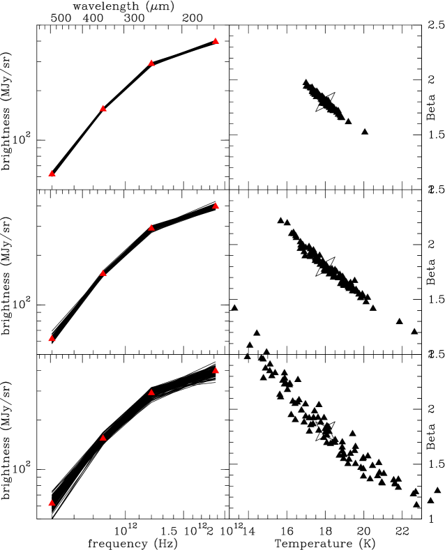
Figure 1: Illustration of the $\beta-T$ degeneracy: the panels on the left hand side show fits to the 4 data points to which noise has been added and the right column shows the values of $\beta$ and T. The large triangles on the left show the original data points (before adding noise) which follow a modified black-body law with $\beta=1.8$ and $T=18$, rather typical values for normal spiral galaxies. The large open stars show this position in the right-hand column. From bottom to top, the noise added follows a Gaussian distribution with standard deviation of 5% (bottom panels), 2% (middle panels) and 1% (top panels). Despite this very low noise level, the scatter in $\beta$ and T is significant and correlated. An enlargement of the spectral coverage, if no other processes like emission from small or spinning dust grains play a role within the extended wavelength range, would help reduce the degeneracy.

A number of authors have found an anti-correlation between $\beta$ and T [e.g. 18]. While many authors [e.g. 48, 73] believe the anti-correlation is not entirely due to the $\beta-T$ degeneracy, it remains difficult to isolate and identify the physical and degenerate parts of this relation [e.g. 22, 61].

Laboratory experiments have also found an anti-correlation between $\beta$ and $T$. However, in space, the anti-correlation is typically for dust temperatures of 10-20 K (the dominant temperatures of dust emitting in the submm) whereas laboratory experiments find the difference between 300 K dust (room temperature) and 10-20 K dust. The difference in dust spectra between 10 K and 20 K is very difficult to identify in laboratory experiments [e.g. 12]. It is currently not clear whether laboratory measurements support a physical $\beta-T$ anti-correlation for dust in the 10-20 K range.

Table 1: Positional data on M33.

Nucleus position (J2000)1	RA = $1^{h}33^{m}51.0^{s}$
	DEC = $30^{\circ}39\arcmin 37.0\arcsec$
Position angle of major axis2	23∘
Inclination3	56∘
Distance4 (1$\arcsec$= 4 pc)	840 kpc
1 [13]
2 [15]
3 [56]
4 [20]

The nearest Scd galaxy, M 33 (NGC 598), at a distance of 840 kpc [1$\arcsec\simeq$ 4 pc, 20] has been extensively studied at IR wavelengths. Its mild inclination [$i=56^{\circ}$, 56, Table 1] makes it a suitable target for mapping a large variety of astrophysical properties. Herschel observations of M 33 (HerM33es, Kramer et al. 2010) enable us to study the dust SED at a resolution where complexes of giant molecular clouds and star forming regions are resolved. Using the Herschel PACS and SPIRE data together with the Multiband Imaging Photometer Spitzer (MIPS) fluxes, [37] studied the dust SED in radial intervals of 2 kpc width (out to 8 kpc galactocentric radius) as well as the integrated SED of M 33. Assuming a constant $\beta$, they found that a two-component MBB fits the SEDs better than the isothermal models. They also showed that the global SED fits better with $\beta$=1.5 than with $\beta$=2. In a pixel-by-pixel approach, [72] derived the temperature and luminosity density distribution of a two-component MBB for the best-fitted $\beta$ of 1.5, which was fixed across the galaxy. This paper investigates possible variations of $\beta$ radially and in the disk of M33, using different single- and two-component MBB approaches in which the degeneracy between $\beta$ and $T$ is treated properly. Studying both single- and two-component MBBs are important to assess the temperature mixing along the line of sight, which could in principle lead to a lower $\beta$ value if a single MBB model is assumed [43]. In order to obtain as much information as possible about the warm dust and to avoid as much as possible contamination by non-thermalized grains (e.g. very small grains), we use the Herschel SPIRE/PACS and Spitzer MIPS maps at wavelengths $\lambda\geq$ 70 $\mu$m, probing primarily the dust emission from the big grains which are believed to be in thermal equilibrium with the interstellar radiation field [see e.g. 7]. In the diffuse Galactic interstellar medium (ISM), these grains emit as a MBB with an equilibrium temperature of $17-18$ K [e.g. 5].

The paper is organized as follows. The data sets used in this study are described in Sect. 2. We present our methods and approaches as well as their resulting physical parameters in Sect. 3. Then, we investigate the systematics of the two-component MBB approaches by performing a Monte-Carlo simulation (Sect. 4). Uncertainties of the physical parameters are presented in Sect. 5. We discuss and summarize the results in Sects. 6 and 7.

Table 2: Images of M 33 used in this study.

Wavelength	Resolution	rms noise	Telescope
500 $\mu$m	$37\arcsec$	8 mJy/beam	Herschel-SPIRE1
350 $\mu$m	$25\arcsec$	9.2 mJy/beam	Herschel-SPIRE1
250 $\mu$m	$18\arcsec$	14.1 mJy/beam	Herschel-SPIRE1
160 $\mu$m	$11\arcsec$	6.9 mJy pix-2	Herschel-PACS2
100 $\mu$m	$7\arcsec$	2.6 mJy pix-2	Herschel-PACS2
70 $\mu$m	$18\arcsec$	10 $\mu$Jy arcsec-2	Spitzer-MIPS3
6570Å (H$\alpha$)	$2\arcsec$	0.3 cm-6 pc	KPNO4
HI-21 cm	$17\arcsec$	50 K km s-1	VLA5
CO(2-1)	$12\arcsec$	0.06 K km s-1	IRAM-30m5
1 [37, 72]
2 [37, 3]
3 [64]
4 [31]
5 [27]

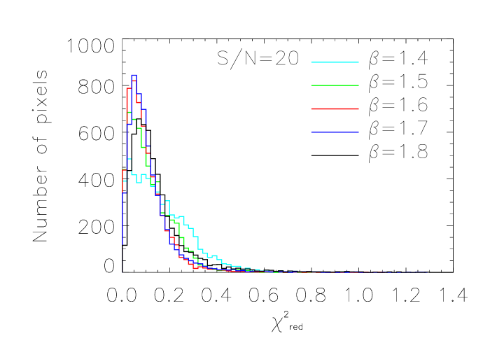
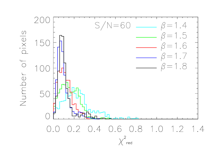
Figure 2: Histogram of the reduced $\chi^{2}$ in the single MBB fitting approach for selected $\beta$ values between 1.4 and 1.8. Results are shown for fits to the high (20$\sigma$, left) and very high (60$\sigma$, right) signal to noise data.

2 Data

Table 2 summarizes the data used in this study. M33 was observed at 250 $\mu$m, 350 $\mu$m, and 500 $\mu$m using the SPIRE photometer [28] onboard the Herschel space telescope. The data were reduced using the Herschel data reduction software HIPE 7.0 as detailed in [72]. We also used the 160 $\mu$m data taken with the Herschel PACS instrument [53]. The PACS data were reduced using the scanamorphos algorithm [58] as discussed in detail in [3]. At shorter wavelengths, we used the 70 $\mu$m Spitzer MIPS data in the two-component MBB approach[64].

The maximum calibration uncertainties (i.e., for diffuse emission) is 15% for the MIPS [7], 20% for the PACS [53], and 15% for the SPIRE bands [28].

We also used H$\alpha$, HI, and CO(2-1) line emission data to investigate the connection between the dust spectrum and tracers of the ionized and neutral gas phases. The CO(2-1) line emission was observed with the IRAM-30m telescope and detailed in [27]. The HI-21 cm line was mapped with the VLA [27]. The H$\alpha$ data is from the Kitt Peak National Observatory (KPNO) [31]. The maps used in our analysis were all convolved to the resolution of the 500 $\mu$m SPIRE image ($\sim 40\arcsec$) by using the dedicated convolution kernels provided by [2] and projected to the same grid of $10\arcsec$ pixel and center position.

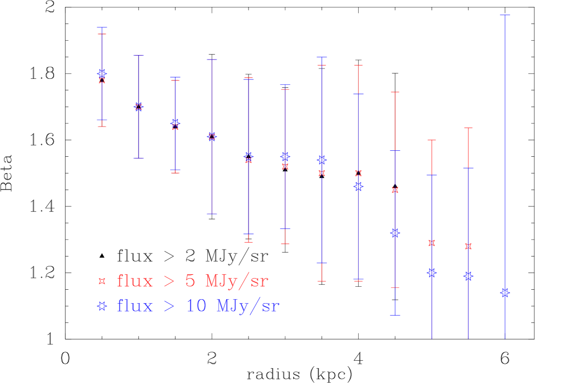
Figure 3: Radial variation of the ‘best-$\beta$’ calculated by minimizing the reduced $\chi^{2}$ for each of the annuli in the single modified black body (MBB) fitting approach (top). The different symbols show a coherent decrease in $\beta$ with radius and represent values obtained for different flux cutoffs as indicated. (Bottom): dust temperature calculated for each flux cutoff at each radius. The error bars show the 1 sigma dispersion.

3 Methodology and Results

We constrain independently $\beta$ and $T$ by using ($a$) single component MBB fits where it is assumed that the grains are described by a fixed $\beta$ but a varying temperature and all physically reasonable values of $\beta$ are tested to see which $\beta$ results in the lowest residuals and ($b$) 2-component MBB models where an iterative method is applied to solve systems of independent equations using the Newton-Raphson method. Approach ($a$) aims to derive $\beta$ and $T$ as a function of the galactocentric radius and to look for trends with FIR luminosity. We derive $\beta$, $T$, and mass surface densities pixel-by-pixel across the galaxy in approach ($b$).

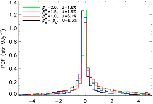
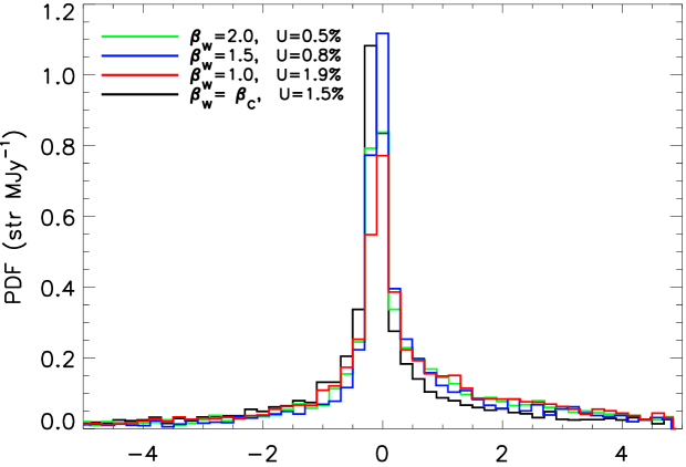
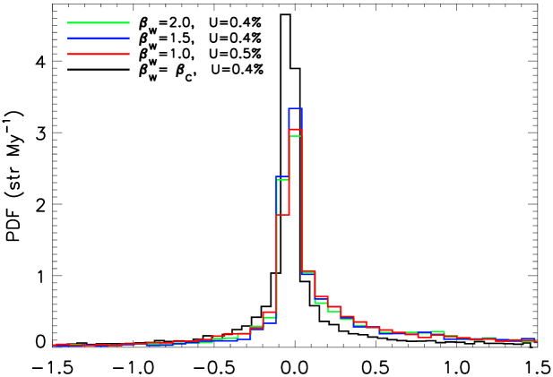
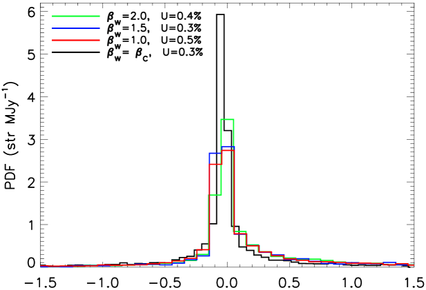
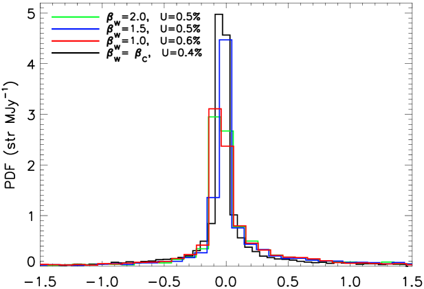
Figure 4: Probability density function (PDF) of residuals between observations and model for the two-component MBB approaches at (from top to bottom) 70, 160, 250, 350, and 500 $\mu$m. The uncertainty of each approach (U) is also given for comparison.

3.1 Single-component approach

In the single-component MBB model (Eq. 1), it is assumed that the grain properties do not change over the region or structure studied so for each pixel we fit only the temperature (and the optical depth, which acts as a general scaling). The temperature is fit for a fixed $\beta$ but we repeat the fitting process for many different values of $\beta$. For a given $\beta$, the overall quality of the fit is determined by minimizing the reduced $\chi^{2}$ as in [72] over the whole set of pixels. This process, while making the hypothesis that $\beta$, representing the grain properties, is unlikely to undergo real variations at the scale of the regions studied, avoids the $\beta-T$ degeneracy while allowing us to determine the ‘best $\beta$’.

For each pixel, fits are first made for the 160-500 $\mu$m bands where cold dust dominates [11]. At 100 $\mu$m, the emission comes from a mixture of cold and warm dust. The observed 100 $\mu$m emission thus represents an upper limit to the emission from the cool component which we fit from 160-500 $\mu$m. If the 100 $\mu$m flux derived from the fit is higher than the observed flux, then we refit using the 100 $\mu$m flux as well, resulting in a more realistic dust temperature.

Exploring the best $\beta$ for a selected set of $\beta$=1, 1.3, 1.5, 1.7 and 2, [72] showed that the data from all wavelengths above the $3\sigma$ rms noise level is best fitted by $\beta$=1.5. Similarly, we explore how the best $\beta$ value varies when selecting progressively higher S/N data. While choosing only high-quality data is desirable as long as enough pixels are available (which is the case), it introduces a selection of regions with more and more star formation and probably also a higher fraction of molecular gas as compared to the lower S/N regions. Comparing to the S/N=3 case [72, see Fig. 3 in], where $\beta=1.5$ yields the lowest residuals, we find that the more actively star-forming high S/N regions have steeper $\beta$, e.g. $\beta=1.6$ for S/N=20 and $\beta=1.7$ for S/N=60 (see Fig. 2).

In order to better investigate the change in $\beta$, we divided M33 into radial bins of 0.5 kpc and made the same calculations for each $\beta$ between 1 and 2.4 with steps of 0.1, looking for the lowest residuals. Figure 3 shows that the best value for $\beta$ decreases with radius from 1.8 to about 1.2. Though differently, the dust temperature also decreases with radius. The higher flux cutoff (10 MJy/sr) has a higher temperature for two reasons. First, at higher fluxes, dust tends to be warmer. Secondly, since the $\beta$ calculated at large radii are lower for the 10 MJy/sr cutoff, the temperatures obtained are higher. These results are very similar to those of Fig. 1 in [66] but using entirely different numerical techniques.

3.2 Two-component approaches

Here we introduce a second dust component heated mainly by young massive stars to a higher temperature (warm dust) in addition to the dust heated by the general interstellar radiation field (ISRF, cold dust). The aim of this approach is to differentiate the dust properties in arm/interarm and inner/outer disk regions, including diffuse emission. Hence, we perform this analysis pixel-by-pixel using the most sensitive Herschel and Spitzer maps available in the wavelength range of 70$\mu$m to 500$\mu$m. The specific intensity of a two-component MBB dust emission is given by

$$S_{\nu} = \,B_{\nu}(T_{c})[1\,-\,exp(-\tau_{\nu,{c}})]$$

$$+\,B_{\nu}(T_{w})[1\,-\,exp(-\tau_{\nu,{w}})],$$

where the indices $c$ and $w$ stand for the cold and warm dust, respectively. The Newton-Raphson iteration method from Numerical Recipes was used to solve the 5 equations corresponding to the five wavelengths at 70, 160, 250, 350, and 500 $\mu$m in order to derive $T_{c}$, $T_{w}$, $\Sigma_{{\rm dust},c}$, $\Sigma_{{\rm dust},w}$, and $\beta$.

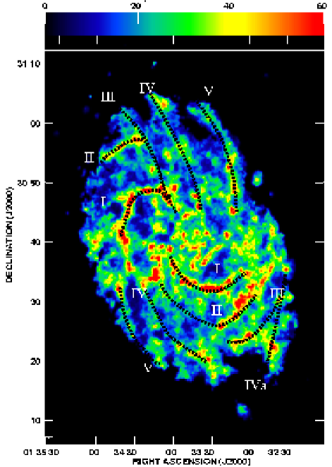
Figure 5: Distribution of the cold dust mass surface density in M33. A sketch of the optical spiral arms [59] is overlaid on top of the cold dust map. The wedge gives the surface density units in $\mu$g cm^-2.

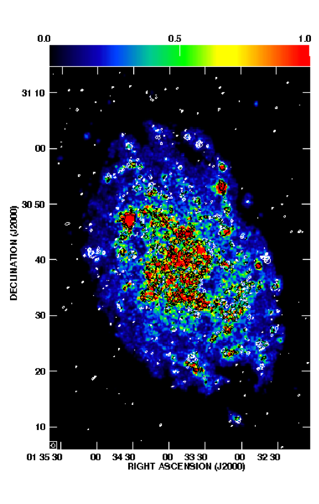
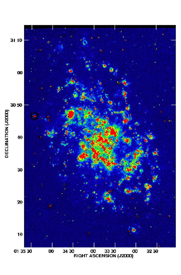
Figure 6: Left: Distribution of the warm dust mass surface density in M33. Overlaid are contours of the H$\alpha$ emission, shown in black or white for a better contrast against background. The wedge gives the surface density units in $\mu$g cm^-2. Right: The H$\alpha$ map of M33.

In order to decrease the probability of falling into a local minimum of the merit function, the initial guess for the physical parameters is determined through synthesizing the observed intensities. We first generate uniform samples of 5000 random sets of variables corresponding to each physical parameter: cold and warm dust temperatures, mass surface densities, and $\beta$. Each random set of physical parameters is then used to synthesize intensities given by Eq. (3) at each wavelength. To define the initial values for the Newton-Raphson method, 20 parameter sets leading to the synthesized intensities closest to the observed values are selected by maximizing the likelihood. Thus, the Newton-Raphson method is applied 20 times for each pixel of the maps resulting in 20 sets of solutions out of which the set minimizing the merit function ($\equiv\sum\frac{(S_{\rm model}-S_{\rm obs})^{2}}{\sigma^{2}_{\rm obs}}$, where $\sigma_{\rm obs}$ is the corresponding calibration uncertainty) was taken as the final set of solutions. The initialization scheme is completely independent for every two pixels. Hence, there is no correlated error due to this procedure.

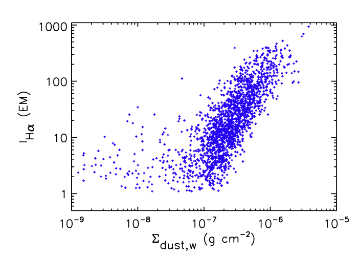
Figure 7: Linear correlation between the warm dust surface density $\Sigma_{{\rm dust},w}$ and the H$\alpha$ emission measure. The scatter in the low surface density tail coincides with the systematic of the approach for this range of surface density (see Sect. 4).

Considering the cold and warm dust, different treatments for $\beta$ are used:
I) Both components of dust are assumed to have the same variable emissivity index ($\beta_{c}=\beta_{w}$=$\beta$).
II) As most of the dust is in the cool phase, the variable $\beta$ is attributed to this major component ($\beta_{c}=\beta$), while the warm dust is assumed to emit with a fixed emissivity index across the disk. Although we are left with a fixed value of $\beta_{w}$ (note that the number of unknowns must be equal to the number of equations), we repeat the analysis for different possibilities of $\beta_{w}$=1, 1.5, and 2.

The above calculations are all performed for every pixel of the maps with intensities higher than the 3$\sigma$ noise level at each wavelength. The pixel-by-pixel analysis further helps to reduce dust temperature mixing as the range of temperatures is limited in a given pixel. Using a Monte-Carlo simulation, the two-component MBB approaches are then synthesized to determine the systematics and reliability of each method.

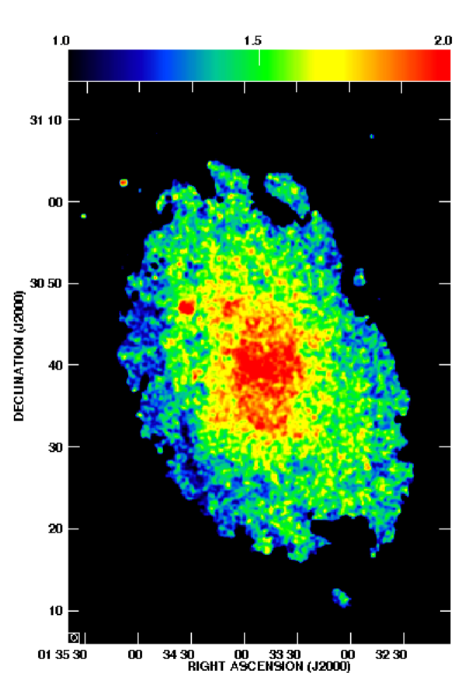
Figure 8: Distribution of the dust emissivity index $\beta$ in the disk of M 33 obtained using the two-component approach with $\beta_{w}$=2.

The temperature and surface density of the cold dust do not depend on the choice of $\beta_{w}$ but the physical parameters of the warm dust are best reproduced using the $\beta_{w}$=2 model (see Sect. 4). This agrees with [8] who derived a mid-infrared power law slope of $\simeq$2 indicative of optically-thin dust with a shallow radial density profile from clumpy, hot regions. Hence, we focus on the results of the two-component MBB with $\beta_{w}$=2, although the general distributions of the physical parameters across the galaxy are similar to those of other two-component MBB models. The PDF (probability density function) of residuals between the observed and modeled intensities (Fig. 4) further shows the preference for the $\beta_{w}$=2 case for the warm dust component as it results in a smaller uncertainty U at 70$\mu$m than the other 2-component MBB models (see the U values in Fig. 4, upper panel).

3.2.1 Distribution of cold and warm dust

Figures 5 and 6 show the resulting distributions of the mass surface densities of the cold and warm dust for the $\beta_{w}$=2 case. The cold dust has been found not only in the main spiral arms (arm I in the north and the south), but also in the weaker arms, flocculent structures and dust lanes. Dense patches of cold dust with surface densities of $\Sigma_{{\rm dust},c}>$ 45 $\mu$g cm^-2 occur along arm I and some parts of arms II and III (in both the north and the south). Moreover, filaments of dense dust have been detected in the central 2.5 kpc. The densest region corresponds to the high concentration of dust in the giant HII/star forming complex NGC 604.

The warm dust is mostly concentrated in the central 2.5 kpc and along the main spiral arm I showing clumpy structures. A good match between clumps of warm dust and star forming/HII regions is found by a comparison with the H$\alpha$ emission (Fig. 6, right). Apart from the central region and the main arms, the rest of the galaxy is covered by many spotty warm dust features, most of them can be found in the H$\alpha$ map as well. Therefore, not only the bright HII regions (like NGC 604, IC 133, NGC 595, NGC 588, and B690) but also the weaker ones can be traced in the warm dust map.

In addition to the tight spatial correlation between H$\alpha$ emission and the warm dust in Fig. 6, Fig. 7 shows that the warm dust column and the H$\alpha$ emission are proportional, with $I_{\rm H\alpha}\propto(0.92\pm\,0.02)\Sigma_{{\rm dust},w}$. The correlation is best (largest Pearson correlation coefficient, see Sect. 6) when $\beta_{w}=2$ and this is one of the reasons for preferring the $\beta_{w}=2$ model over $\beta_{w}=1$ and 1.5. The Monte-Carlo simulation presented in Sect. 4 provides further support for $\beta_{w}=2$.

The average mass surface density of the warm dust in star forming complexes in the central 4 kpc is $\Sigma_{{\rm dust},w}=0.8\pm 0.3\,\mu$g cm^-2. The cold-to-warm dust mass ratio has a gaussian distribution (in log) which peaks at $\sim$100, typical of spiral galaxies [45, 67], and a standard deviation of one order of magnitude. We stress that this result is derived without any pre-assumption about the filling factor of the cold or warm dust.

3.2.2 Distribution of the dust emissivity index $\beta$

Figure 8 shows that $\beta$ varies between 1.2 and 2 across the galaxy, in agreement with Fig. 3. The mean value of the dust emissivity index over the disk is $\beta=1.5\pm\,0.2$. This is in agreement with $\beta$ derived globally by [37] using the integrated SED and [72] by exploring the best $\beta$ described in Sect. 3.1. As in the inner disk, a steep dust spectrum with $\beta\simeq 2$ is found in NGC604. Out to NGC 604, the main spiral arms are visible in the $\beta$ map having a higher index ($\beta>$1.5) than their adjacent inter-arm regions with smaller $\beta$. This confirms the higher $\beta$ for the high S/N cutoffs derived for these radii in the single-component MBB approach (Sect. 3.1). All over the $\beta$ map, there are small-scale fluctuations with variations of $\lesssim$0.2 which could be due to noise or systematics of the approach (Sects. 4 and 5).

3.2.3 Cold and warm dust temperatures

The temperatures of both cold and warm dust components are in general lower in the outer disk than in the inner disk of M33. In the central 4 kpc, the cold dust temperature $T_{c}$ varies mainly between 20 K and 24 K with an average of 21$\pm$2 K (Figs. 9 and 3). In the outer parts, $T_{c}$ ranges between 14 K and 19 K with a mean value of 17$\pm$2 K. The higher cold dust temperature in the inner disk with respect to the outer disk is consistent with [37, 6, 72]. A similar trend was also found in other disk galaxies based on Herschel data [e.g. 54, 19, 21]. The corresponding $T_{c}$ values in HII regions agree with those derived by [57] using [17] models and following the prescription of [22]. Warm dust temperatures of $T_{w}\gtrsim$50 K are found in the spiral arms and star forming regions with a maximum of 60$\pm$10 K in NGC 604, NGC 595, and IC 133. In the outer parts, the warm dust has a temperature of $T_{w}=35\pm 10$ K on the average (the errors given are discussed in Sect. 5).

Based on the physical parameters retrieved, the modelled SEDs are shown for two selected pixels with different $\beta$ in Fig. 10.

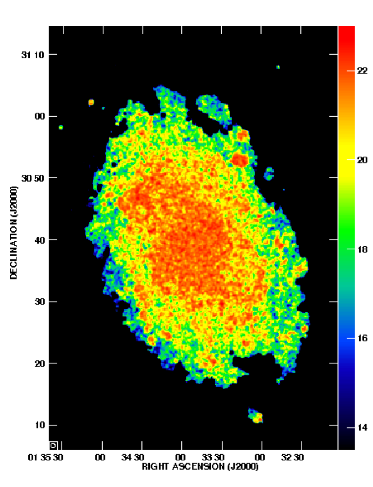
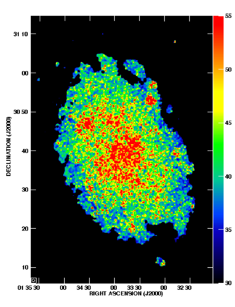
Figure 9: Distribution of the cold (left) and warm (right) dust temperatures in M33. The wedge shows the temperature values in Kelvin.

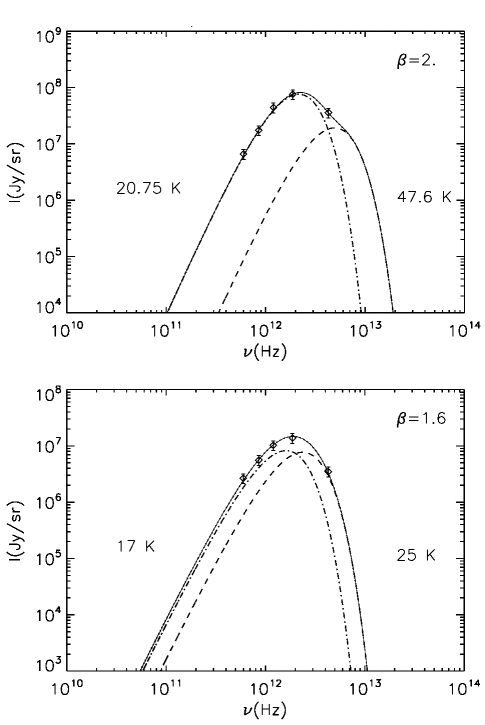
Figure 10: Modelled dust SED for the two-component modified black body for 2 different pixels with coordinates RA=1^h 33^m 31.35^s, DEC=$30:30:21.18$ (top) and RA=1^h 33^m 17.31^s, DEC=$30:21:47.99$ (bottom). The dashed, dot-dashed, and solid curves represent the SEDs of the warm, cold, and total dust emission, respectively.

4 Monte-Carlo simulations with the Newton-Raphson method

Using a Monte-Carlo simulation, we assess the systematics and reliability of the two-component approaches. This is particularly useful to check for an artificial correlation between $\beta$ and $T$. The Monte-Carlo simulations are performed assuming a uniform probability density function. We first generate random numbers for each of the physical parameters in a selected range given in Table 3. For surface densities, we use a uniform distribution in logarithmic space. The extreme values in the selected ranges may seem far from reality. Compared to more moderate values, however, this selection ensures that we cover the whole physical parameter space. Each set of physical parameters generated (input) leads to synthesized intensities using Eq. (3) as described in Sect. 3.2. The synthesized intensities are then treated as observed data in the Newton-Raphson method resulting in new sets of physical parameters (output). In the ideal case, i.e. when there are no systematics due to a specific model or approach, the output parameters are similar to the input parameters. This case is indicated by a one-to-one (equality) relation between the input and output parameters in Figs. 11 and 12.

In all the two-component MBB models, the simulations show that $T_{c}$ can be best reproduced between 10 K and 20 K and the scatter around the equality relation is symmetric for the $\beta_{w}=2$ case (other models tend to overestimate $T_{c}$). In this case, $T_{c}$ is reproduced with an accuracy better than 3 K in the range 10-20 K. This case also shows a symmetric scatter for $T_{w}$ for 35 K $<T_{w}<$ 50 K, where it is best reproduced (with a dispersion of 11 K), while other models tend to underestimate $T_{w}$ in this range. The mass surface density of the cold dust shows generally a small scatter for all models and it is much better constrained than that of the warm dust. The accuracy of reproducing the dust mass surface density is about 5.5 times better for the cold than the warm component in logarithmic scale for the $\beta_{w}=2$ case. This case is again more successful in reproducing $\Sigma_{{\rm dust},w}$ than other cases, especially for mass surface densities $\Sigma_{{\rm dust},w}<10^{-6}$ g cm^-2. Interestingly, we find a coincidence between the low density scatter in the H$\alpha$–$\Sigma_{{\rm dust},w}$ correlation plot (Fig. 7) and the low density deviations in the simulated $\Sigma_{{\rm dust},w}$ (Fig. 12). Where $T_{c}<$10 K and $\Sigma_{{\rm dust},c}>10^{-5}$ g cm^-2, there are points that follow a shallower slope than the equality relations. These points are likely local minima in the merit algorithm. Synthesizing the observed data, however, reduces the chance of falling into a local minimum, as explained in Sect. 3.2.

Figure 11 shows that $\beta$ is not as well constrained as $T_{c}$. To give an example, for an input value of $\beta$=1.5 (with $\beta_{w}$=2), the output value of $\beta$ varies between 1.1 and 2 with a dispersion of 0.3. The method tends to overestimate $\beta$ for $\beta<$1.5 and underestimate it for $\beta>$2.

To study the sensitivity of the different MBB approaches to noise, we add Gaussian noise with a width of 5$\sigma$ rms of the observed maps to the synthesized intensities at various wavelengths and re-run the simulations. Adding the noise increases the dispersion in $\beta$ by $\sim$50% in the two-component MBB with $\beta_{w}=2$. It is important to note that none of the model approaches lead to an artificial correlation between temperature, mass surface density, and $\beta$ for both simulated and real results (see Fig. 13 and Sect. 5.1).

Table 3: Setup of the numerical experiment in the two-component MBB approaches.

Approach	Tc [K]	Tw [K]	$\log$($\Sigma_{{\rm dust},c}$) [g cm-2]	$\log$($\Sigma_{{\rm dust},w}$)[g cm-2]	$\beta$	Statistics
$\beta_{w}$=1	5$-$25	26$-$70	(-6)$-$(-3)	(-9)$-$(-5)	0.8$-$2.5	15 000
$\beta_{w}$=1.5	5$-$25	26$-$70	(-6)$-$(-3)	(-9)$-$(-5)	0.8$-$2.5	15 000
$\beta_{w}$=2	5$-$25	26$-$70	(-6)$-$(-3)	(-9)$-$(-5)	0.8$-$2.5	15 000
$\beta_{w}$= $\beta_{c}$	5$-$25	26$-$70	(-6)$-$(-3)	(-9)$-$(-5)	0.8$-$2.5	15 000

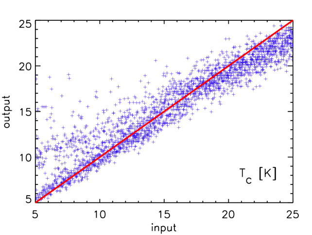
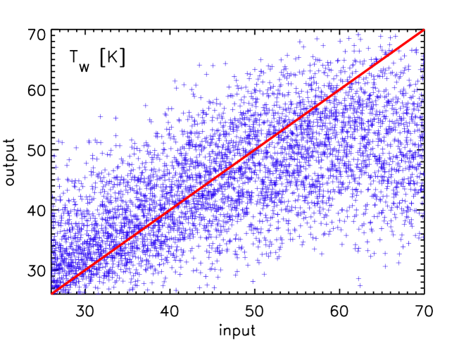
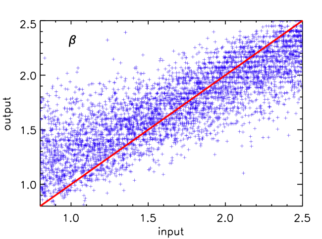
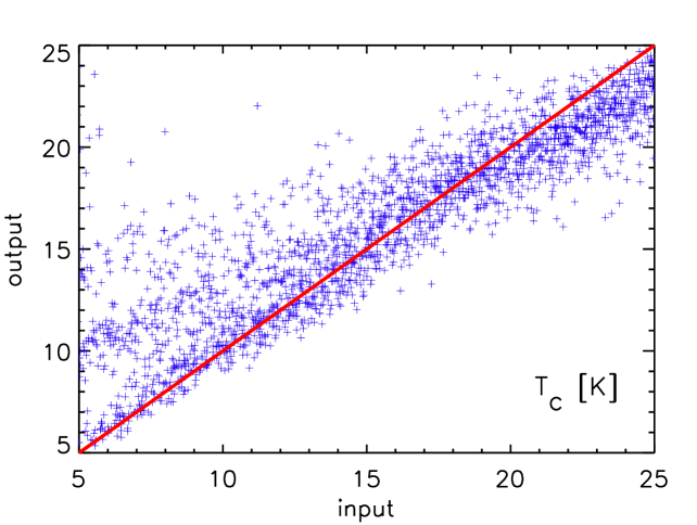
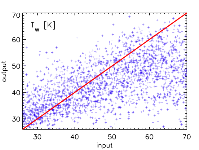
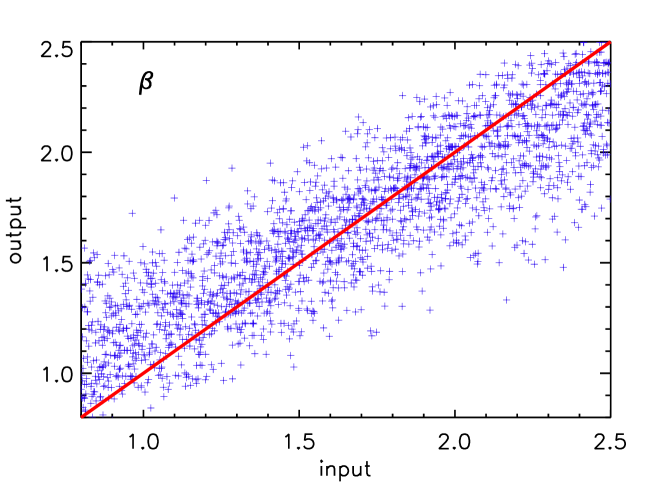
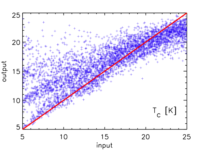
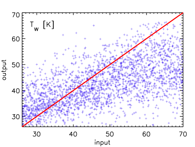
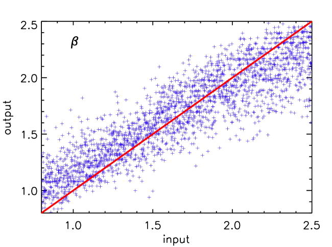
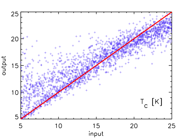
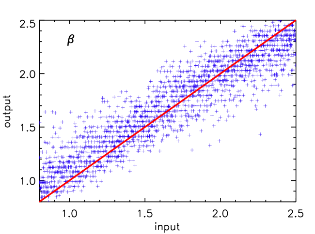
Figure 11: Monte-Carlo simulation of the two-component MBB model. From left to right: $T_{\rm c}$, $T_{\rm w}$, and $\beta_{c}(=\beta)$. From top to bottom: $\beta_{w}=2$, $\beta_{w}=1.5$, $\beta_{w}=1$, and $\beta_{w}=\beta_{c}$. The red line shows the equality between the output and input parameters.

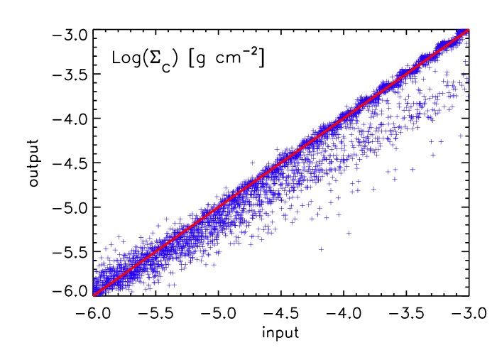
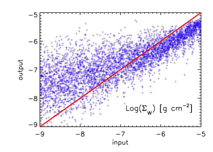
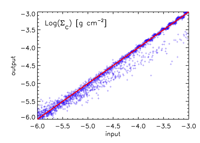
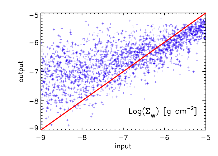
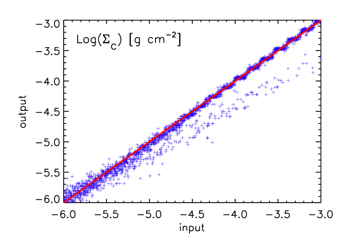
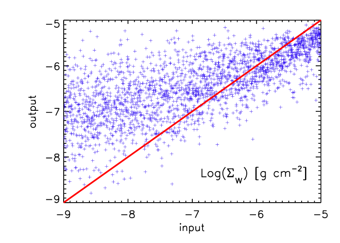
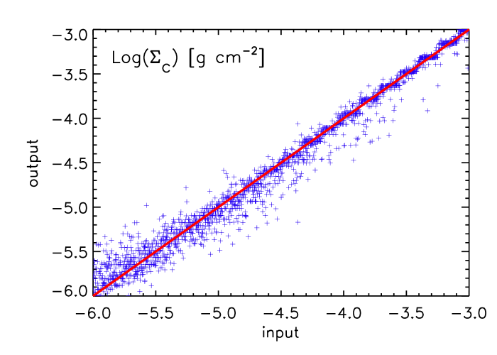
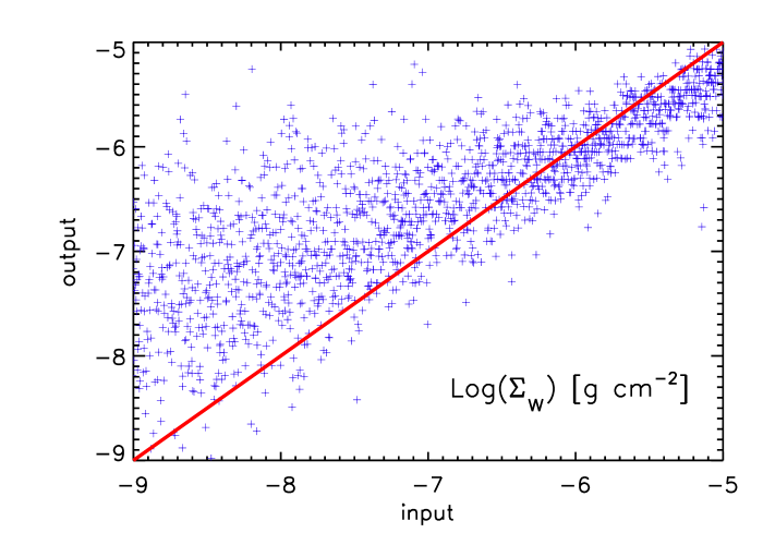
Figure 12: Monte-Carlo simulation of the two-component MBB model. Left: $\Sigma_{{\rm dust},c}$ and right: $\Sigma_{{\rm dust},w}$. From top to bottom: $\beta_{w}=2$, $\beta_{w}=1.5$, $\beta_{w}=1$, and $\beta_{w}=\beta_{c}$. The red line shows the equality between the output and input parameters.

5 Sources of uncertainties

In addition to the uncertainties due to the method, our results could be affected by statistical and systematic uncertainties on measured fluxes. To study the effect of the statistical uncertainties, we first measure the stochastic pixel noise by calculating the dispersion in intensities in background regions. In the reduced images, background dispersion could in principle be due to the propagation of original pixel noise and artifacts into the background pixels as well as possible imperfect foreground subtraction. We then simulated the observed intensities by adding random noise with normal distribution of 3$\sigma$ background noise level measured at each wavelength. Using this statistical experiment, we created 1000 mock datasets used as the data points (fluxes) in our two-component approach with $\beta_{w}=2$ resulting in a set of 1000 values for each physical parameter. The statistical uncertainties ($\delta_{\rm stat}$) were then determined from the standard deviation of the results (Table 4).

Table 4: Uncertainties of the obtained physical parameters.

Parameter	$\delta_{\rm sys}$	$\delta_{\rm stat}$	$\delta$
Tc [K]	2.0	0.1	2.0
Tw [K]	10.0	2.3	10.3
log($\Sigma_{{\rm dust},c}$) [dex]	0.08	0.00	0.08
log($\Sigma_{{\rm dust},w}$) [dex]	0.54	0.34	0.64
$\beta$	0.22	0.01	0.22

The flux uncertainty could also be due to systematic uncertainties, e.g., calibration errors and artifacts caused by observing cameras [e.g. 1], which do not have the same properties as the statistical errors. In most cases, systematics are addressed via calibration uncertainties, as the systematics due to cameras are not well-defined. For NGC 6946 and NGC 0628, [1] investigated the systematics due to the MIPS and PACS cameras by comparing their data at a same wavelength (after convolving them to the same resolution and pixel size). For M33, such a comparison is possible only at 160$\mu$m, as at other wavelengths the data are taken with only one camera. We consider the relative difference in the 160$\mu$m intensities obtained with MIPS and PACS as an estimate for the systematic error if it is larger than the calibration uncertainty at each pixel. In the region of interest $R<6$ kpc (inside the optical radius $R_{25}\sim 7.5$ kpc), the relative difference between the MIPS and PACS data is $\lesssim$ 20%, which is comparable to the calibration uncertainty. Hence, the systematics at 160$\mu$m are dominated by the calibration uncertainty. We assume a similar situation for the data at other wavelengths. This is supported by using the maximum calibration uncertainties at each wavelength (Sect. 2). The uncertainties in the physical parameters due to the systematics are then determined by adding the calibration uncertainties (see Sect. 2) to the synthesized intensities retrieved in the Monte-Carlo experiment in Sect. 4. These intensities were then used to derive the physical parameters using the Newton-Raphson method. This way the systematics due to the method are also taken into account. Table 4 shows the median of the absolute residuals ($\rvert$output -input$\rvert$), $\delta_{\rm sys}$.

The error on each physical parameter is then given by $\delta=\sqrt{\delta^{2}_{\rm sta}+\delta^{2}_{\rm sys}}$. As expected, $\delta$ is dominated by the systematics rather than the statistical noise.

To evaluate the role of the systematics on the decrease of $\beta$ with distance from the center shown in Sect. 3.2.2, yet another experiment is performed. After adding the systematic uncertainties to the observed intensities, a vertical cut passing through the center of M 33 was solved 100 times using the Newton-Raphson method. This resulted in 100 sets of solutions for each pixel along the vertical cut. The uncertainties in the physical parameters are then determined from the standard deviations of the parameter distributions. Fig. 14 (left) shows the distribution (profile) of $\beta$ and its uncertainty $\delta\beta$ along the cut. From the center to $R\simeq\,6$ kpc (indicated by the blue lines), $\delta\beta$ increases from $\simeq$ 0.15 to $\simeq$ 0.3. This is equivalent to a relative change in $\beta$ from $\simeq$ 6% to $\simeq$ 20% as shown in Fig. 14 (right). Hence, the magnitude of the derived radial decrease of beta is significant, i.e. larger than three times the uncertainty.

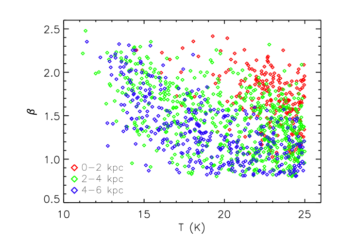
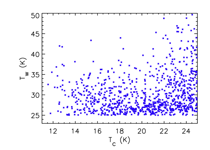
Figure 13: Up: scatter plot of the cold dust emissivity index $\beta$ vs. temperature, colour-coded for three radial intervals. Bottom: scatter plot of the cold dust temperature vs. the warm dust temperature showing no correlation.

6 Discussion

6.1 The $\beta$–$T$ correlation

One of the most important results of this work is that we clearly show that not only the temperature but also $\beta$ decreases with galactocentric distance in M 33. This is a real effect, shown by different physical and numerical approaches and because the effect is strong enough to be seen against the well-known numerical $\beta-T$ anti-correlation [62].

The techniques adopted in this work – solving a system of equations or deriving the ‘best-$\beta$’ leaving only the temperature as a variable – are robust despite the strength of the $\beta-T$ degeneracy. However, for any given pixel there is a tendency for $\beta$ and $T$ to be anti-correlated simply because dust temperatures derived with lower $\beta$ are higher, whatever the method. When averaged over radial annuli, it becomes clear that both $\beta$ and $T$ decrease with radius , though their decreasing trends are not similar (e.g. Fig. 3).

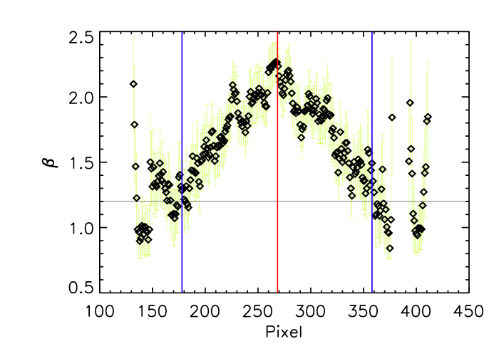
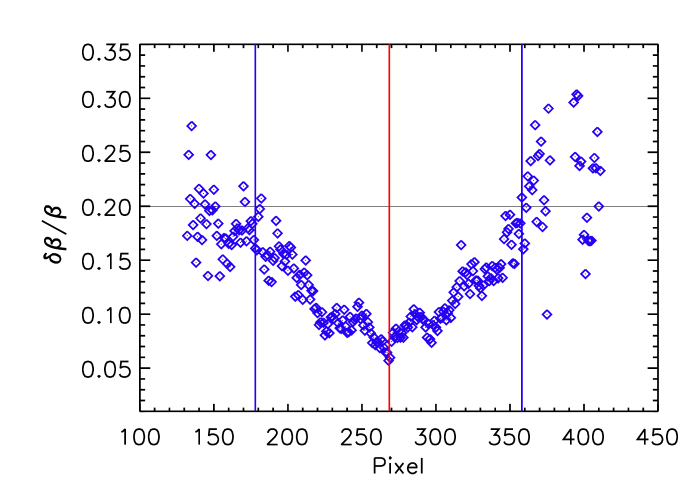
Figure 14: Distribution of the emissivity index $\beta$ (right) and its relative uncertainty $\delta\beta$ /$\beta$ (left) along a vertical cut passing through the center. The red and blue lines indicate the center of M 33 and $R\simeq$ 6 kpc, respectively.

In M31, with similar data and thus similar linear resolution as for M33, [63] find that $T$ and $\beta$ have opposite behavior as a function of radius (their Fig. 8), such that the temperature increases with radius and $\beta$ decreases. This may be linked to the $\beta-T$ degeneracy because the dust temperature decreases with radius in M31 as shown by [21] using the same data and in other studies [29, 65].

It is already known that the dust temperature decreases with radius in M33 due to the radial decrease in the interstellar radiation field at all wavelengths [69, 37, 6, 3, 72]. A trend of decreasing $\beta$ could only be expected if $\beta$ is also linked to a factor which varies (on average) with radius.

In addition to the ISRF, many properties of spiral galaxies vary with distance from the center: the metallicity decreases with radius as does the H₂/HI ratio, the stellar surface density, and the star formation rate. Thus, the gradient in $\beta$ we find could be due to any of these factors, among which the metallicity, the H₂/HI ratio, and the star formation rate are strongly linked. This motivates us to look for a correlation between $\beta$ and different environmental conditions imposed by star formation activity and different phases of the ISM.

6.2 Connection to star formation and ISM tracers

Within the inner disk, the spiral arms and NGC 604 are visible as high-$\beta$ regions (Fig. 8). In both Fig. 3 and Fig. 8, a clear change in $\beta$ is apparent at 4 kpc radius, where $\beta$ changes from approximately Galactic [$\beta\simeq 1.8$, 50] to lower than that of the LMC [$\beta\simeq 1.5$, 51]. This is also the radius at which [26] noticed a break in the H₂ formation efficiency in M33 (see their Fig. 13). Starting at the same radius, the [CII]/FIR ratio is also found to increase [36].

In Fig. 15, we investigate possible connections between the observed $\beta$ and star formation, via the H$\alpha$ brightness, the CO(2-1) and the HI line emission. After excluding pixels with a signal-to-noise ratio smaller than 3, the maps of the H$\alpha$, CO(2-1), and HI integrated intensities were used to perform cross-correlation with $\beta$ in the same way as in Sect. 5.1. Figure 15 shows that $\beta$ is higher in regions with star formation as traced by H$\alpha$ emission (top panel). The link between $\beta$ and the molecular gas (middle panel), which is the fuel for star formation, is slightly weaker and in agreement with the observation that most but not all molecular clouds in M33 host star formation [27]. The atomic gas surface density is only poorly linked to the current star formation and there is no clear correlation between HI surface density and $\beta$ (lower panel). The fact that, unlike H$\alpha$ emission and molecular gas, the atomic gas is not concentrated in the central disk and along the spiral arms could explain the weak $\beta$–HI correlation obtained.

Since both H$\alpha$ and molecular gas trace star formation, this indicates that the dust spectrum could differ in starforming and non-starforming regions. Star formation could in principle influence the grain composition and size distribution (via shattering of dust grains due to strong shocks or dust coagulation), which could modify the dust emissivity index $\beta$. Although such a difference has not been proven, it is possible that the properties of the dust in the atomic and molecular gas clouds differ due to the temperature and density differences.

Star formation replenishes the ISM with metals e.g. through stellar winds of young massive stars and supernovae. Concerning the dust grains, this is likely to increase the abundance ratio of silicates to carbonaceous grains [71]. According to the standard dust models, $\beta$=2 is consistent with silicate grains, while $\beta$=1 for carbonaceous grains [e.g. 14]. Observations of the Milky Way show that silicates dominate the ISM [e.g. 47, 46, crystalline silicates however are not found much in the diffuse ISM] which is consistent with the observed dust emissivity index of close to 2 [$\beta\simeq 1.8$ 50]. Galaxies with lower metallicity than the Milky Way, however, are found to have flatter SEDs [e.g. 25, 51], indicating the general role of metal abundance on the dust emissivity variation. Similarly, M33, which has a sub-solar metallicity by about a factor of 2 [42], shows a flatter average value of $\beta$ ($\sim 1.5$), higher in the central 4 kpc and lower in the outer parts. The fact that most of the young massive stars are concentrated in the central 4 kpc of M33, while the evolved carbon stars are smoothly distributed over the disk [e.g. 69], could provide a distinct difference in the dust composition and hence the emissivity index.

The dust grains in the ISM are subject to a variety of destruction and modification processes like vaporization, shattering, and coagulation with the latter two processes being more important in the ISM [e.g. 68, 34]. Shattering and fragmentation of dust grains occurs in grain-grain collisions caused by shocks which can shift the peak in the grain size distribution to smaller values [34] and may change crystalline grains into amorphous [70], leading to a flatter SED [60]. The small grains are more dominant in the diffuse and low-density ISM, considering that they have been accelerated by shock waves traversing the ISM, than in the spiral arms with sites of grain growth in dense molecular clouds.

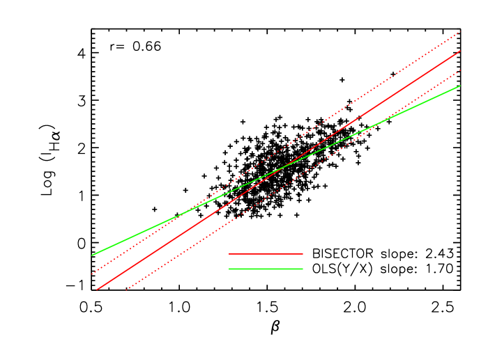
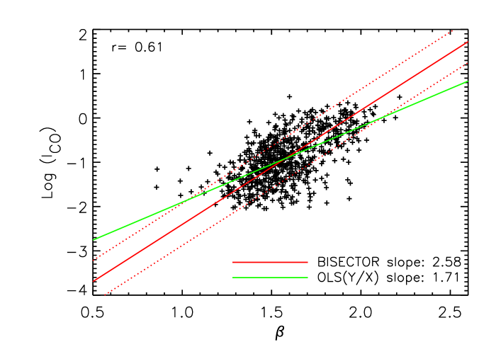
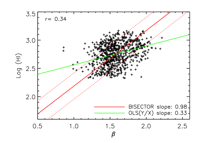
Figure 15: Scatter plots of the dust emissivity index $\beta$ versus the H$\alpha$, CO(1-0), and HI emission from M33. The y-axis presents the logarithm of the intensities in units of cm^-6 pc for the H$\alpha$ emission and K km $s^{-1}$ for the CO(1-0) and HI emssions. Also shown are Pearson correlation coefficients (r), the ordinary least square (OLS) fits, and the bisector fits.

We note the possibility of systematic deviations of the calculated $\beta$ values from the true $\beta$. As shown in Sect. 4, the dynamical range in the true (intrinsic) $\beta$ could be larger than that obtained in the 2-component MBB approach. The $\beta$ values smaller than $\sim$1.5 could be overestimated and those larger than $\sim$2 underestimated. The true variation in $\beta$ may be greater than that shown in Fig. 8.

In our observations, as in likely all astrophysical situations, the dust within the telescope beam is not at a single temperature. The emission spectrum of dust at similar but different temperatures is necessarily broader than single-temperature dust and, if fit by a single MBB, the resulting $\beta$ will be lower than for the real grains. This however depends strongly on the density [43].

Could the temperature mixing be particularly dominant for the outer disk of M 33, leading to the radial decrease in $\beta$ that we find? We have several arguments that suggest this is not the case.
- Firstly, it would appear somewhat counter-intuitive to have the broader mix of dust temperatures where there are fewer dust grains (the dust surface density is considerably lower in the outer disk), particularly with respect to the central regions. This agrees with [43], showing that the observed $\beta$ is closer to the true $\beta$ in regions with lower dust densities. A smaller temperature variation in the outer than the inner parts is already visible in Fig. 10 by comparing $T_{c}$ and $T_{w}$ in each of those regions.
 -Secondly, several flux cut-offs were used for the single-component model (Fig. 3) and irrespective of the cutoff a clear gradient in $\beta$ is observed. Selecting pixels with strong fluxes, we select outer disk regions with a level of star formation similar to what is observed in the inner disk and indeed the dust is fairly warm. However, these pixels have a low $\beta$. Similarly, using the two-component model, the two hot giant HII regions in the outer parts, IC 131 and IC 133, appear as weak sources in the $\beta$ map (Fig. 8), unlike the HII regions in the inner disk.
-Thirdly, not only the single-component but also the two-component MBB model, which is designed to disentangle the temperature mixing at first order of approximation, leads to a radial decrease in $\beta$. Comparing $\beta$ from the two methods, it is deduced that the single-component method indeed leads to a smaller $\beta$, particularly in the center. However, the difference in $\beta$ is not larger in the outer than in the inner disk (see Fig. 16, showing the difference in $\beta$ obtained from the two methods vs. radius).

Figure 16: Difference in the dust emissivity index $\beta$ derived using the two-component MBB and the single-component MBB models vs. radius.

7 Summary

Using the Herschel SPIRE/PACS and Spitzer MIPS maps at $\lambda\geq$ 70 $\mu$m, we investigate the physical properties of dust using single and two-component modified black body models and study the variation of the dust emissivity index $\beta$ across M 33. Although the single and two-component models use modified black-bodies, the procedures are very different and both have been designed to avoid the $\beta-T$ degeneracy. The single-component model assumes that $\beta$ does not vary rapidly from pixel to pixel at the scale observed in M33 (160 pc) and, by testing many values of $\beta$, determines the value leading to the lowest residuals. The two-component models solve exactly for the parameters ($T$, $\beta$, surface density) for a combination of warm and cold dust for data covering 70 $\mu$m to 500 $\mu$m whereas the single component models use the data from 160 $\mu$m to 500 $\mu$m.

Both analyses find that ($i$) $\beta$ is higher in actively star forming regions, ($ii$) $\beta$ is higher in the inner disk and decreases sharply beyond a galactocentric distance of 4 kpc, and of course ($iii$) that the dust temperature decreases with radius. Both $\beta$ and $T$ decrease with radius in M33, contrary to reported anti-correlations.

In addition, the two component model shows that within the inner disk, $\beta$ is higher along the spiral arms. The warm dust follows the H$\alpha$ emission, indicating that the separation into warm and cold dust is appropriate. Proper behavior of the two-component model has also been verified by extensive Monte-Carlo simulations.

In an attempt to identify the reason for the variation of $\beta$, we find that $\beta$ is correlated both with H$\alpha$ intensity and with CO(2-1) line strength but not significantly with the HI column density. As CO and H$\alpha$ emission decrease radially, we are not able to distinguish their effects on $\beta$. The radial decrease in $\beta$ appears not to be due to an increasingly broad mixture of dust temperatures.