Asteroseismological study of massive ZZ Ceti stars with fully evolutionary models

Abstract

We present the first asteroseismological study for 42 massive ZZ Ceti stars based on a large set of fully evolutionary carbon$-$oxygen core DA white dwarf models characterized by a detailed and consistent chemical inner profile for the core and the envelope. Our sample comprise all the ZZ Ceti stars with spectroscopic stellar masses between $0.72$ and $1.05M_{\odot}$ known to date. The asteroseismological analysis of a set of 42 stars gives the possibility to study the ensemble properties of the massive pulsating white dwarf stars with carbon$-$oxygen cores, in particular the thickness of the hydrogen envelope and the stellar mass. A significant fraction of stars in our sample have stellar mass high enough as to crystallize at the effective temperatures of the ZZ Ceti instability strip, which enables us to study the effects of crystallization on the pulsation properties of these stars. Our results show that the phase diagram presented in Horowitz et al. (2010) seems to be a good representation of the crystallization process inside white dwarf stars, in agreement with the results from white dwarf luminosity function in globular clusters.

1 Introduction

ZZ Ceti (or DAV) stars are the most numerous class of degenerate pulsators, with $\sim 160$ members known to date (Castanheira et al. 2013a). These stars have hydrogen atmospheres and are located in a narrow range in effective temperature $10\,500\mathrel{\hbox{\hbox to0.0pt{\hbox{\lower 4.0pt\hbox{$\sim$}}\hss}\hbox{$<$}}}T_{\rm eff}\mathrel{\hbox{\hbox to0.0pt{\hbox{\lower 4.0pt\hbox{$\sim$}}\hss}\hbox{$<$}}}12\,300$ K (e.g. Fontaine & Brassard 2008; Winget & Kepler 2008; Althaus et al. 2010a), mostly with temperatures close to the center of the instability strip, and masses $\sim 0.6M_{\odot}$ (Gianninas, Bergeron & Fontaine 2005: Castanheira & Kepler 2008). Their photometric variations are due to spheroidal, non-radial $g$-mode pulsations with low harmonic degree ($\ell\leq 2$) and periods in the range 70$-$2000 s, with amplitude variations of up to 0.3 mag. The driving mechanism thought to excite the pulsation near the blue edge of the instability strip is the $\kappa-\gamma$ mechanism acting on the hydrogen partial ionization zone (Dolez & Vauclair 1981; Winget et al. 1982). The “convective driving mechanism” proposed first by Brickhill (1991) and later revisited by Goldreich & Wu (1999) is thought to become dominant once a thick convective zone has developed in the outer layers.

The ZZ Cetis can be classified into three groups, depending on the effective temperature (Mukadam et al. 2006, Clemens et al. 1993). The hot ZZ Cetis, that define the blue edge of the instability strip, and exhibit a few modes with short periods ($<350$ s) and small amplitudes (1.5-20 mma). The pulse shape is sinusoidal or sawtooth shaped and is stable for decades. On the opposite side of the instability strip we have the cool DAV stars, showing several long periods (up to 1500 s), with large amplitudes (40-110 mma), and non sinusoidal light curves that can change dramatically from season to season due to the mode interference. Finally, Mukadam et al. (2006) suggested introducing a third class, the intermediate ZZ Cetis, that exhibit mixed characteristics from hot and cool DAV stars. Recently, Hermes et al. (2012, 2013a) extended the variability strip of pulsating DAV stars to cooler temperatures with the discovery of low mass pulsators. The variable low mass white dwarf stars are characterized by effective temperatures below $\sim 10\,000$ K and long periods in the range $1000-4500$ s.

Over the years, pulsation studies of ZZ Ceti stars through asteroseismology have become a valuable technique to study the details of the origin, internal structure and evolution of white dwarfs (Winget & Kepler 2008; Fontaine & Brassard 2008, Althaus et al. 2010a). In particular, the thickness of the outer envelope, the chemical composition of the core, magnetic fields and rotation rates can be determined from the observed periods. Also the rate of period change can be employed to measure their cooling rate (Kepler et al. 2005) and to study particles like neutrinos (Winget et al. 2004) or axions (Isern et al. 1992: Córsico et al. 2001; Bischoff-Kim et al. 2008; Isern et al 2010; Córsico et al. 2012ab) and the possible rate of variation of the Newton constant (Córsico et al. 2013), but also to look for extrasolar planet orbiting these stars (Mullally et al. 2008). In addition, asteroseismology of white dwarf stars is a valuable tool to place observational constraints on the crystallization process in the very dense interiors of white dwarf stars (Montgomery & Winget 1999; Córsico et al. 2004, 2005; Metcalfe et al. 2004; Kanaan et al. 2005).

The number of white dwarf stars, and consequently of ZZ Ceti stars, has dramatically increased with the Sloan Digital Sky Survey (SDSS) project (Mukadam et al. 2004; Mullally et al. 2005; Kepler et al. 2005, 2012; Castanheira et al. 2006, 2007, 2010, 2013a). In particular, Kleinman et al. (2013) reported $12\,843$ DA and 923 DB white dwarfs stars from the SDSS Data Release 7 (Abazajian et al. 2009). The mass distribution for DA white dwarf stars presented by Kleinman et al. (2013) shows a main components with stellar mass around $\sim 0.59M_{\odot}$, that comprise $\sim 80\%$ of the total sample, and also a low$-$mass and a high$-$mass components. The main population of high$-$mass white dwarfs has masses above 0.721$M_{\odot}$ and peaks at 0.822 $M_{\odot}$. It is thought that most of the white dwarf stars populating the high-mass component are likely to have carbon$-$oxygen cores, formed during the stable helium burning phase in the pre$-$white dwarf evolution. However, evolutionary computations show that stars with stellar mass in the Zero Age Main Sequence (ZAMS) of $\mathrel{\hbox{\hbox to0.0pt{\hbox{\lower 4.0pt\hbox{$\sim$}}\hss}\hbox{$>$}}}7M_{\odot}$ reach stable carbon ignition giving rise to an oxygen$-$neon or an oxygen$-$neon$-$magnesium core white dwarf star with stellar mass larger than $\sim 1.05M_{\odot}$ (Ritossa et al. 1999; Siess 2007). Therefore, the massive component of the DA white dwarf mass distribution is populated by carbon$-$oxygen core stars, with a progenitor star of $\sim 3-7M_{\odot}$, as well as oxygen$-$neon core white dwarf stars with stellar mass above $\sim 1.05M_{\odot}$, resulting from a progenitor star with masses between $\sim 7-8.5M_{\odot}$ .

High$-$mass white dwarf stars are not easy to find, not only because their intrinsically smaller number with respect to lower mass white dwarfs, but also because they evolve fast and have low luminosity due to their smaller radius. Therefore, the search for variable high$-$mass white dwarfs is quite challenging. The most studied massive DAV star is BPM 37093 with $M_{*}=1.1\pm 0.05M_{\odot}$, discovered to be variable by Kanaan et al. (1992). Because of its high mass, BPM 37093 was considered the only pulsator to have undergone partial crystallization and thus presented the opportunity to study the crystallization theory through asteroseismology (Metcalfe et al. 2004; Kanaan et al. 2005). In the past few years, pulsation variability have been searched for and detected in several other massive DAV stars (Kepler et al. 2005; Castanheira et al. 2006; Castanheira et al. 2010; Kepler et al. 2012, Castanheira et al. 2013a), but only a few of these objects have been analyzed using asteroseismology. The first attempt to study the general properties of massive DAV stars has been presented recently by Castanheira et al. (2013a). In addition to report the discovery of five new massive pulsators and perform seismological fits for these particular objects, they carried out a study of the observational properties of a set of massive pulsating DA stars with spectroscopic stellar mass higher than $0.8M_{\odot}$. They choose only 25 stars with SDSS spectra in order to have an homogeneous sample in terms of atmospheric determinations (Kleinman et al. 2004, Kleinman et al. 2013).

Currently, there is no asteroseismological study in the literature applied specifically to the massive variable white dwarfs as a group. This paper is intended to fill this gap. Specifically we perform an asteroseismological analysis of all massive DA variable white dwarf stars known to date, with spectroscopic masses in the range $0.72-1.05M_{\odot}$. Note that the stellar mass values in the target selection include only massive DAVs expected to have carbon$-$oxygen cores. We defer the study of very massive DAVs thought to harbor oxygen$-$neon core DAVs, like the classical BPM 37093 (Kanaan et al. 1998; Metcalfe et al. 2004) and the recently discovered GD 518 (Hermes et al. 2013b), for a future paper as our current evolutionary models are not appropriate. Our sample of massive DAV stars is composed by 42 objects, 36 of which were discovered within the SDSS DR7 (Kleinman et al. 2013), 5 objects are bright ZZ Ceti stars (e.g. Fontaine & Brassard 2008), and one was selected from the SuperCOSMOS Sky Survey catalog (Rowell & Hambly 2011). Most of these stars have observational data only from the discovery paper with only a few modes detected, in many cases a single mode. To perform our seismological study we employ a grid of full evolutionary models representative of white dwarf stars discussed in Romero et al. (2012) which have consistent chemical profiles for both the core and the envelope for various stellar masses, particularly intended for detailed asteroseismological fits of ZZ Ceti stars. The chemical profiles of our models are computed from the full and complete evolution of the progenitor stars from the ZAMS, through the thermally pulsing and mass$-$loss phases on the asymptotic giant branch (AGB). We consider the ocurrence of extra$-$mixing episodes during all stages prior to the thermally pulsing AGB, and time$-$dependent element diffusion during the white dwarf stage (Althaus et al. 2010b, Renedo et al. 2010). Our asteroseismological approach combines $(i)$ a significant exploration of the parameter space $(M_{*},T_{\rm eff},M_{\rm H}$) and $(ii)$ a detailed and updated input physics, in particular, regarding the internal structure, that is a crucial aspect for correctly disentangle the information encoded in the pulsation patterns of variable white dwarfs. The first version of this model grid was employed by Romero et al. (2012) to perform an asteroseismological study of a sample of 44 bright ZZ Ceti stars with stellar masses $\simeq 0.5-0.8M_{\odot}$, including G117$-$B15A. In this paper we present a second version of the model grid, where we extended our parameter space towards higher stellar mass values. In addition, we include different treatments of the crystallization process in our computations, as an extra parameter in our model grid.

The paper is organized as follows. In Section 2 we describe the evolutionary code and the input physics adopted in our computations and we present the model grid employed in our asteroseismological study. Section 3 is devoted to study the effects of crystallization process on the pulsation spectrum of massive white dwarf stars. In Section 4 we present our sample of massive DA variable white dwarfs and quote their properties from spectroscopy. Section 5 briefly introduces new observations performed for a few objects from our sample. In Section 6 we present our results from the asteroseismological procedure. We conclude in Section 7 by summarizing our findings.

2 Numerical tools and models

2.1 Input physics

The grid of full evolutionary models employed in this work were calculated with an updated version of the LPCODE evolutionary code (see Althaus et al. 2005a; Althaus et al. 2010b; Renedo et al. 2010 for details). Here, we comment the main input physics relevant for this work. Further details can be found in those papers.

The LPCODE evolutionary code considers a simultaneous treatment of no$-$instantaneous mixing and burning of elements (Althaus et al. 2003). The nuclear network accounts explicitly for 16 elements and 34 nuclear reactions, that include $pp-$chain, CNO$-$cycle, helium burning and carbon ignition (Renedo et al. 2010). In particular, the ¹²C$(\alpha,\gamma)^{16}$O reaction rate, of special relevance for the carbon$-$oxygen stratification of the resulting white dwarf, was taken from Angulo et al. (1999). As a consequence, our white dwarf models are characterized by systematically lower central oxygen abundances than the values found by Salaris et al. (1997), who use the larger rate of Caughlan et al. (1985) for this reaction.

Also, we consider the occurrence of extra$-$mixing episodes beyond each convective boundary following the prescription of Herwig et al. (1997), except for the thermally pulsating AGB phase. The occurrence of extra$-$mixing episodes during the core helium burning phase largely determines the final core chemical composition of the resulting white dwarf (Straniero et al. 2003). We treated the extra$-$mixing (overshooting) as a time dependent diffusion process — by assuming that the mixing velocities decay exponentially beyond each convective boundary — with a diffusion coefficient given by $D_{\rm EM}=D_{0}\exp(-2z/fH_{P})$, where $H_{P}$ is the pressure scale height at the convective boundary, $D_{O}$ is the diffusion coefficient of unstable regions close to the convective boundary, and $z$ is the geometric distance from the edge of the convective boundary (Herwing et al. 1997, 2000). The free parameter $f$ describes the efficiency of the extra$-$mixing process. It can take values as high as $f\sim 1.0$, for overadiabatic convective envelopes of DA white dwarfs (Freytag et. al 1996). However, for deep envelope and core convection $f$ is expected to be considerably smaller because the ratio of the Brunt$-$Väisälä timescales of the stable to unstable layers decrease with depth. In this study we have assumed f = 0.016, which accounts for the location of the upper envelope on the main sequence for a large sample of clusters and associations (Schaller et al. 1992, Herwig et al. 1997, 2000). Also it accounts for the intershell abundances of hydrogen$-$deficient post$-$AGB remnants (see Herwig et al. 1997; Herwig 2000; Mazzitelli et al. 1999). Finally, for the mass range considered in this work the mass of the outer convection zone on the tip of the RGB only increases by $\sim 1.5\%$ if we change the parameter $f$ by a factor of two. The suppression of extra$-$mixing events during the thermally pulsating AGB phase prevents the third dredge$-$up to occur in low mass stars (Lugaro et al. 2003; Herwig et al. 2007; Salaris et al. 2009), leading to the gradual increase of the hydrogen free core mass as evolution proceeds during this phase. As a result, the initial$-$final mass relationship by the end of the thermally pulsating AGB is markedly different from that resulting from considering the hydrogen free core mass right before the first thermal pulse. In fact, Althaus et al. (2010b) demonstrated that, depending on the stellar mass of the white dwarf, the central oxygen abundances can be underestimated up to a $\sim$15% if the white dwarf mass is taken as the mass of the hydrogen free core at the first thermal pulse. Finally, the breathing pulse instability occurring towards the end of the core helium burning are usually attributed to the adopted algorithm rather than to the physics of convection and therefore were suppressed in our computations (see Straniero et al. 2003 for a more detailed discussion).

We considered mass loss during the core helium burning and the red giant branch phases following Schröder & Cuntz (2005), and during the AGB and thermally pulsating AGB following the prescription of Vasiliadis & Wood (1993). Since there is a strong reduction of the third dredge$-$up, as is the case of the sequences computed in this work, mass loss plays an important role in determining the final mass of the hydrogen free core at the end of the thermally pulsating AGB evolution, and thus the initial$-$final mass relation. However, the residual helium burning in a shell, that increases the core mass during the thermally pulsating AGB and the hot stages of the white dwarf evolution, is also important in determining the white dwarf final mass.

During the white dwarf evolution, we consider the distinct physical process that modify the chemical abundances distribution. In particular, element diffusion strongly affects the chemical composition profile throughout the outer layers. Indeed, our sequences developed a pure hydrogen envelope with increasing thickness as evolution proceeds. Our treatment of time$-$dependent diffusion is based on the multicomponent gas treatment presented in Burgers (1969). We consider gravitational settling and thermal and chemical diffusion of $\textonesuperior$H, ³He, ⁴He, ¹²C, ¹³C, ¹⁴N and ¹⁶O (Althaus et al. 2003). To account for convection process we adopted the mixing length theory, in its ML2 flavor, with the free parameter $\alpha=1.61$ (Tassoul et al. 1990). Finally, we considered the chemical rehomogenization of the inner carbon$-$oxygen profile induced by Rayleigh$-$Taylor instabilities following Salaris et al. (1997).

The input physics of the code include the equation of state of Segretain et al. (1994) for the high density regime complemented with an updated version of the equation of state of Magni & Mazzitelli (1979) for the low density regime. Other physical ingredients considered in LPCODE are the radiative opacities from the OPAL opacity project (Iglesias & Rogers 1996) supplemented at low temperatures with the molecular opacities of Alexander & Ferguson (1994). During the white dwarf cooling, the metal mass fraction $Z$ is specified consistently according to the predictions of chemical diffusion. Conductive opacities are those from Cassisi et al. (2007), and the neutrino emission rates are taken from Itoh et al. (1996) and Haft et al. (1994). It is worth mentioning that the presence of rotation during the pre$-$white dwarf evolution may affect the chemical structure and the evolutionary properties of the models. For instance Georgy et al. (2013), based on a large grid of rotating and non$-$rotating MS models, found that rotation induces an increase in the MS lifetimes of about 20$-$25% for models with initial mass larger than 1.7 $M_{\odot}$. Also there is a nitrogen enrichment at the end of the MS for models with rotation. On the other hand, the final mass for rotating models is similar to that for non$-$rotating models.

Cool white dwarf stars are expected to crystallize as a result of strong Coulomb interactions in their very dense interior (van Horn 1968). Crystallization occur when the energy of the Coulomb interaction between neighboring ions is much larger than their thermal energy. This occurs when the ion coupling constant $\Gamma\equiv\langle Z^{5/3}\rangle e^{2}/a_{\rm e}k_{\rm B}T$ is larger than certain value, which depends on the adopted phase diagram. Here $a_{\rm e}$ is the interelectronic distance, $\langle Z^{5/3}\rangle$ an average (by number) over the ion charges, and $k_{\rm B}$ Boltzmann’s constant. The rest of the symbols have their usual meaning. The occurrence of crystallization leads to two additional energy sources: the release of latent heat and the release of gravitational energy associated with changes in the chemical composition of carbon$-$oxygen profile induced by crystallization (García$-$Berro et al. 1988ab, Winget et al. 2009). In our study, the inclusion of these two additional energy sources was done self$-$consistently and locally coupled to the full set of equations of stellar evolution, were the luminosity equation is appropriately modified to account for both the local contribution of energy released from the core chemical redistribution and the latent heat. At each timestep, the crystallization temperature and the change of the chemical profile resulting from phase separation are computed using the appropriate phase diagram. In particular, the carbon enhanced convectively unstable liquid layers overlying the crystallizing core are assumed to be instantaneously mixed, a reasonable assumption considering the long evolutionary timescales of white dwarfs (Isern et al. 1997). The chemical redistribution due to phase separation has been considered following the procedure described in Montgomery et al. (1999) and Salaris et al. (1997). To assess the enhancement of oxygen in the crystallized core we employed two phase diagrams: the spindle$-$type phase diagram of Segretain & Chabrier (1993) and the azeotropic$-$type phase diagram of Horowitz et al. (2010) (see Althaus et al. 2012 for details on the implementation). In our computations, crystallization begins for $\Gamma\sim 180$ when we employ the Segretain & Chabrier (1993) phase diagram and for $\Gamma\sim 220$ when we consider the Horowitz et al. (2010) phase diagram. For pure carbon crystallization occurs when $\Gamma=178.4$. After computing the chemical composition of both the solid and the liquid phases, we evaluated the net energy released in the process as in Isern et al. (1997). This energy is added to the, usually smaller, latent heat contribution, of the order of $0.77k_{B}T$ per ion. Both energy contributions were distributed over a small mass range around the crystallization front.

2.2 Model grid

The DA white dwarf models employed in this work are the result of full evolutionary calculations of the progenitor stars, from the ZAMS, through the hydrogen and helium central burning stages, thermally pulsating and mass loss in the AGB phase and finally the planetary nebula domain. They were generated employing LPCODE evolutionary code. The metallicity value adopted in the Main Sequence models is $Z=0.01$. Most of the sequences with masses $\leq 0.878M_{\odot}$ were employed in the asteroseismological study of 44 bright ZZ Ceti stars by Romero et al. (2012), and were extracted from the full evolutionary computations of Althaus et al. (2010b) (see also Renedo et al. 2010). In this work we extend the model grid towards the high mass domain. We computed five new full evolutionary sequences with initial masses on the ZAMS in the range $5.5-6.7M_{\odot}$ resulting in white dwarf sequences with stellar masses between $0.917$ and $1.024M_{\odot}$. In addition, we compute two new sequences with white dwarf masses of 0.721 and 0.800 $M_{\odot}$ in order to achieve a finer coverage of the low mass region of our sample. Finally, we obtained a sequence with a stellar mass 1.050 $M_{\odot}$ by artificially scaling the stellar mass from the 0.976$M_{\odot}$ sequence at high effective temperatures (Córsico et al. 2004). The values of stellar mass of our complete model grid are listed in column 1 of table LABEL:tabla-grid, along with the hydrogen (column 2) and helium (column 3) content as predicted by standard stellar evolution, and the carbon ($X_{\rm C}$) and oxygen ($X_{\rm O}$) central abundances by mass in columns 4 and 5, respectively. The values of stellar mass of our set of models accounts for the stellar mass of all the observed pulsating DA white dwarf stars with a probable carbon$-$oxygen core. Note that white dwarfs with masses higher than 1.05 $M_{\odot}$ probably have oxygen$-$neon cores, since they reach off$-$center carbon ignition in partial electron degenerate conditions before entering the white dwarf cooling sequence.

Our parameter space is build up by varying three quantities: stellar mass ($M_{*}$), effective temperature ($T_{\rm eff}$) and thickness of the hydrogen envelope ($M_{\rm H}$). Both the stellar mass and the effective temperature vary in a consistent way with the expectations from evolutionary computations. On the other hand, we decided to vary the thickness of the hydrogen envelope in order to expand our parameter space. The choice of varying $M_{\rm H}$ is not arbitrary, since there are uncertainties related to mass loss rates during the AGB phase leading to uncertainties on the amount of hydrogen remaining on the envelope of white dwarf stars. For instance, Althaus et al. (2005b) have found that the amount of hydrogen left in a DA white dwarf can be significantly reduced if the progenitor star experience a late thermal pulse. Tremblay & Bergeron (2008) show that a broad range in the thickness of the hydrogen envelope can lead to the observed increase in the He$-$ to H$-$rich white dwarfs, although the mixing has to occur for temperatures lower than $\sim 10\,000$ K (Tremblay et al. 2010). Recently, Kurtz et al. (2013) reported the discovery of a member of the so called “hot DAV” stars in the cooler edge of the DB gap, whose pulsation instability was predicted by Shibahashi (2005, 2007) based on the possible existence of very thin hydrogen envelope DA white dwarfs ($M_{\rm H}\sim 10^{-12}M_{*}$). The remaining amount of hydrogen in a white dwarf also depends on the metallicity adopted for the progenitor star. Renedo et al. (2010) show that, for a $\sim 0.6M_{\odot}$, the thickness of the hydrogen envelope increases by a factor of $\sim 2$ when the metallicity of the progenitor star is reduced from $Z=0.01$ to $Z=0.001$.

Other structural parameters are not thought to change considerably according to standard evolutionary computations. For instance, Romero et al. (2012) showed that the remaining helium content of DA white dwarf stars cannot be substantially lower (as much as 3$-$4 orders of magnitude) than that predicted by standard stellar evolution, and only at the expense of an increase in the the hydrogen free core ($\sim 0.2M_{\odot}$). The structure of carbon$-$oxygen chemical profiles are basically fixed by the evolution during the core helium burning stage and are not expected to vary during the following single evolution (we do not consider possible merger episodes)

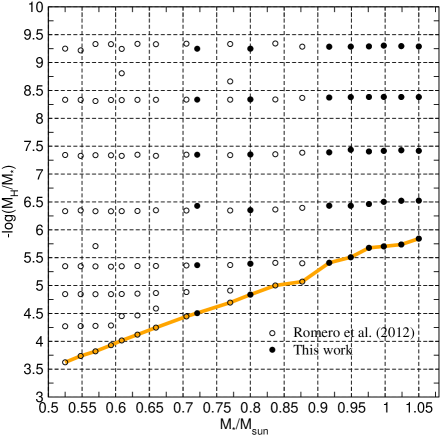
Figure 1: The grid of 163 DA white dwarf evolutionary sequences considered in this work in the $M_{*}-\log(M_{\rm H}/M_{*})$ plane. Each circle corresponds to a sequence of models representative of white dwarf stars characterized by a given stellar mass and hydrogen envelope mass. Open circles correspond to the evolutionary sequences computed in Romero et al. (2012), while filled circles correspond to sequences computed in this work. The orange thick line connects the sequences with the maximum values of the thickness of the hydrogen envelope, predicted by our evolutionary computations.

In order to get different values of the thickness of the hydrogen envelope, we follow the procedure described in Romero et al. (2012). Briefly, for each sequence with a given stellar mass and a thick H$-$envelope, as predicted by the full computation of the pre-white dwarf evolution (column 2 in Table LABEL:tabla-grid), we replaced ¹H with ⁴He at the bottom of the hydrogen envelope. This is done at high effective temperatures ($\mathrel{\hbox{\hbox to0.0pt{\hbox{\lower 4.0pt\hbox{$\sim$}}\hss}\hbox{$<$}}}90\,000$ K), so the transitory effects caused by the artificial procedure are completely washed out when the model reaches the ZZ Ceti instability strip. The resulting values of hydrogen content for different envelopes are shown in Figure 1 for each mass. The orange thick line connects the values of $M_{\rm H}$ predicted by standard stellar evolution (column 2 table LABEL:tabla-grid). Note that the maximum value of the hydrogen envelope shows a strong dependence on the stellar mass. It ranges from $2.4\times 10^{-4}M_{*}$ for $M_{*}=0.525M_{\odot}$ to $1.4\times 10^{-6}M_{*}$ for $M_{*}=1.050M_{\odot}$, with a value of $\sim 1\times 10^{-4}M_{*}$ for $M_{*}\sim 0.60M_{\odot}$. Computations from Romero et al. (2012) are depicted with open circles while computations done in this work are indicated as filled circles. In addition, for sequences with masses between 0.878 and 1.050 $M_{\odot}$ and all the values of the hydrogen envelope mass, we computed three evolutionary sequences with different treatments of the crystallization process and the additional energy sources related to it: (1) considering the release of latent heat and the release of gravitational energy due to phase separation using the phase diagram given by Horowitz et al. (2010), (2) the same as the former case but considering the phase diagram given by Segretain & Chabrier (1993), and (3) considering the release of latent heat but neglecting chemical redistribution due to phase separation. Thus, we can consider the crystallization treatment as a kind of extra parameter on our model grid. To our knowledge, this is the first time that the crystallization process is taken into account self consistently with these different prescriptions in an asteroseismological study of white dwarfs. Our goal is to use asteroseismology of massive white dwarfs to ascertain which treatment is favored. We devote Section 3 to study the effects of crystallization on the pulsation spectrum of massive carbon$-$oxygen mass white dwarf stars, and discuss the results from our asteroseismological fits. In closing, we mention that by adding the evolutionary sequences computed in this work ($\sim 80$) to those computed in Romero et al. (2012), we have available a grid of $\sim 170$ evolutionary sequences, widely covering the mass range in which carbon$-$oxygen white dwarfs are supposed to be.

2.3 Pulsation computations

We computed nonradial $g-$mode pulsations of our complete set of massive carbon$-$oxygen core white dwarf models employing the adiabatic version of the LP-PUL pulsation code described in Córsico & Althaus (2006). The pulsation code is based on the general Newton$-$Raphson technique that solves the full fourth order set of equations and boundary conditions governing linear, adiabatic, nonradial stellar pulsations following the dimensionless formulation of Dziembowski (1971). We used the so called “Ledoux modified” treatment to asses the run of the Brunt$-$Väisälä frequency ($N$) (see Tassoul et al. 1990), generalized to include the effects of having three different chemical components varying in abundance. This code is coupled with the LPCODE evolutionary code. In order to account for the effects of crystallization on the pulsation spectrum of $g-$modes we have appropriately modified the pulsation code considering the inner boundary conditions. In particular, we adopted a “hard sphere” boundary condition, that assumes that the amplitude of the eigenfunctions of $g-$modes is drastically reduced below the solid/liquid interface due to the non$-$shear modulus of the solid, as compared with the amplitude in the fluid region (Montgomery & Winget 1999). In our code, the inner boundary condition for the population of crystallized models is not the stellar center but instead the mesh$-$point corresponding to the crystallization front moving towards the surface (see Córsico et al. 2004; 2005 for details).

The asymptotic period spacing is computed as in Tassoul et al. (1990):

$$\Delta\Pi_{\ell}=\frac{2\pi^{2}}{\sqrt{\ell(\ell+1)}}\left(\int_{r_{1}}^{r_{2}}\frac{N}{r}dr\right)^{-1}$$ (1)

where $N$ is the Brunt$-$Väisälä frequency, and $r_{1}$ and $r_{2}$ are the radii of the inner and outer boundary of the propagation region, respectively. Note that when a fraction of the core is crystallized, $r_{1}$ coincides with the radius of the crystallization front, which is moving outwards as the star cools down, and the fraction of crystallized mass increases. Hence, the integral in eq. (1) decreases, leading to an increase in the asymptotic period spacing, and also in the periods themselves.

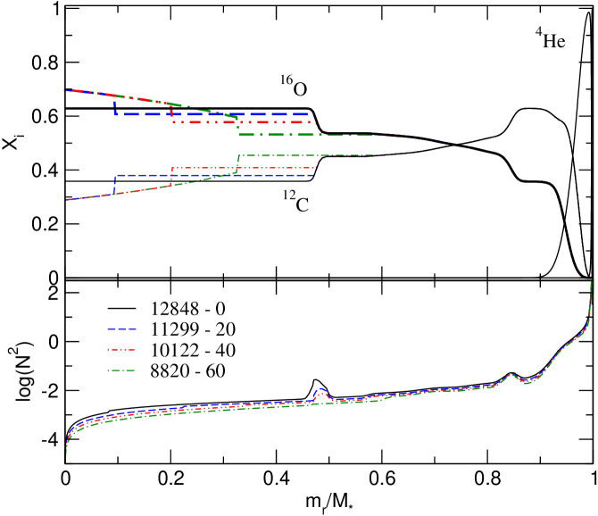
Figure 2: Internal chemical profiles (upper panel) and the logarithm of the square of the Brunt$-$Väisälä frequency (lower panel), in terms of the mass coordinate, corresponding to a DA white dwarf model with $0.998M_{\odot}$ at different stages of the cooling evolution. In this case, we consider the energy release of latent heat and phase separation upon crystallization according to Horowitz et al. (2010). Thick lines depict the oxygen chemical distribution, while thin lines depict the carbon abundance profile. For each model, the effective temperature and percentage of crystallized mass are indicated.

In Figure 2 we plot the inner chemical profiles (upper panel) and the logarithm of the square of the Brunt-Väisälä frequency (lower panel), for models with $M_{*}=0.998M_{\odot}$ and different values of effective temperature. This sequence belongs to computations where we employ the phase diagram given in Horowitz et al. (2010). The percentage of crystallized mass present in the model is indicated along with the effective temperature.

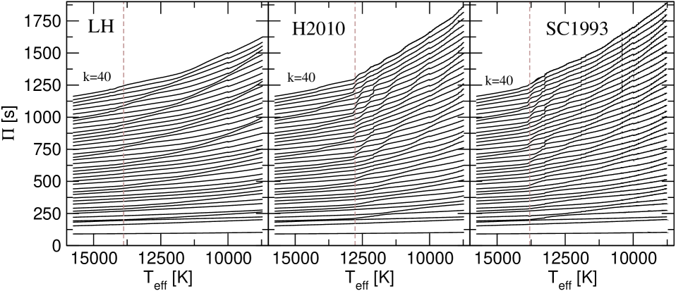
Figure 3: Evolution of the periods for $\ell=1$ modes with $k=1-40$ as a function of the effective temperature, corresponding to a sequence with $M_{*}=0.998M_{\odot}$ and canonical H envelope. Left panel: model where phase separation upon crystallization was neglected. Middle panel: result for H2010 phase diagram. Right panel: computation considering SC1993 phase diagram. The vertical line shows the value of $T_{\rm eff}$ when crystallization sets in.

Each chemical transition region leaves an imprint on the shape of the Brunt-Väisälä frequency, and consequently on the theoretical period spectrum (Althaus et al. 2003). In the core region, the presence of a pronounced step at $m_{r}/M_{*}\sim 0.49$, which is a result of the occurrence of extra$-$mixing episodes during central helium burning, leads to a narrow bump on the Brunt$-$Väisälä frequency profile. When crystallization finally sets in ($\sim 12\,800$ K for this stellar mass), rehomogenization due to phase separation modifies the structure of the carbon and oxygen abundances in the central region. As the crystallization front moves outwards, the carbon$-$oxygen chemical transition at $m_{r}/M_{*}\sim 0.49$ becomes smoother, leaving a weaker feature on the Brunt$-$Väisälä frequency. The feature related to this transition disappears for effective temperatures around $\sim 9\,000$ K (see lower panel of Figure 2). Additional features in the Brunt-Väisälä frequency are related to a oxygen/carbon/helium chemical transition region, product of nuclear burning during the AGB and thermally pulsating AGB stages, and to the outer helium/hydrogen transition (see, for instance, Figure 3 in Romero et al. 2012). These chemical interfaces are modified by diffusion process acting during the cooling evolution. In particular, the oxygen/carbon/helium chemical transition is usually quite wide and mode$-$trapping effects due to this transition are not expected to be too strong, as compared to other chemical interfaces. The outer helium/hydrogen chemical transition is also a source of mode trapping associated with modes trapped in the outer envelope. The features induced on the Brunt-Väisälä by the oxygen/carbon/helium and helium/hydrogen chemical transitions will have a strong influence on the properties of the period spectrum. In particular, they determine the mode$-$trapping properties of DA white dwarf stars models (Bradley & Winget 1991, Brassard et al. 1992, Córsico et al. 2002). Summarizing, we computed the theoretical pulsation spectrum for about $\sim 32\,600$ DA white dwarf models. We varied three structural parameters: the stellar mass in the range $0.721\leq M_{*}/M_{\odot}\leq 1.050$, the effective temperature in the range $\sim 15\,000-9\,000$ K, and the thickness of the hydrogen envelope in the range $-9.4\leq\log(M_{\rm H}/M_{*})\leq-4.5$, where the range of the values of $M_{\rm H}$ depends on the stellar mass. In addition, for sequences with stellar mass $\geq 0.878M_{\odot}$, for which crystallization might occur at the effective temperatures considered, we computed the theoretical pulsation spectrum considering three different treatments of the crystallization process. For each model we computed the adiabatic oscillation spectrum with harmonic degrees $\ell=1$ and 2 and periods in the range 80$-$2000 s.

3 Crystallization process in white dwarf stars

One of the additions we have done to the first model grid presented in Romero et al. (2012) is to include different treatments of the crystallization process in our computations. Specifically, for sequences with stellar masses higher than $\sim 0.878M_{\odot}$, we computed the white dwarf evolution employing three different treatments of crystallization. i.e. by using the phase diagrams from Horowitz et al. (2010) and Segretain & Chabrier (1993), and by only taking into account the release of latent heat as an additional energy source. In this section we study the impact of crystallization process on the theoretical pulsation spectrum of massive DAV white dwarfs. We analyze the main differences between the considered crystallization treatments on the pulsation properties and on the periods themselves.

3.1 Phase diagrams for dense carbon$-$oxygen mixtures

As it is known since Abrikosov (1960), Kirzhnitz (1960) and Salpeter (1961) a white dwarf star evolving on the cooling track, eventually will crystallize as a result of the strong Coulomb interactions in their very dense interior. Crystallization gives rise to two additional energy sources: latent heat (van Horn 1968) and the release of gravitational energy due to phase separation in the carbon$-$oxygen core (García$-$Berro et al. 1988ab). As the oxygen$-$enriched solid core grows at the center of the white dwarf, the lighter carbon$-$rich liquid mantle left behind is efficiently redistributed by Rayleigh$-$Taylor instabilities (Isern et al. 1997). This process release gravitational energy, and this additional energy source has a substantial impact in the computed cooling times of cool white dwarfs (Segretain et al. 1994; Salaris et al. 1997; Montgomery et al. 1999; Salaris et al. 2000; Isern et al. 2000; Renedo et al. 2010; Althaus et al. 2012).

For several years, the standard phase diagram for crystallization used in the stellar evolutionary computations of white dwarf stars was that presented in Segretain & Chabrier (1993). These authors used a density$-$functional approach to obtain a phase diagram for an arbitrary dense binary ionic mixture. For a carbon$-$oxygen mixture these authors obtained a phase diagram of the spindle type, strongly dependent on the charge ratio. Recently, the phase diagram of dense carbon$-$oxygen mixtures appropriate for white dwarf star interiors has been re-examined by Horowitz et al. (2010). This work was motivated by the results of Winget et al. (2009) who found that the crystallization temperature for white dwarfs stars in the globular cluster NGC 6397 was compatible with the theoretical luminosity function for $0.5-0.535M_{\odot}$ white dwarfs and pure carbon cores. Horowitz et al. (2010) used molecular dynamic simulations involving the liquid and solid phases simultaneously, allowing a direct determination of the melting temperature and the composition of the liquid and solid phases from a single simulation. These authors predict an azeotopic type phase diagram, and melting temperature considerably lower than that predicted by Segretain & Chabrier (1993). In fact, they conclude that constraining the melting temperature of white dwarfs cores to be close to that for pure carbon from Segretain & Chabrier (1993) computations, the oxygen concentration should be around $\mathrel{\hbox{\hbox to0.0pt{\hbox{\lower 4.0pt\hbox{$\sim$}}\hss}\hbox{$<$}}}60\%$. Schneider et al. (2012) use the same technique as in Horowitz et al. (2010) based on larger simulations with a larger number of ions and also included a more accurate identification of liquid, solid and interface regions using a bond angle metric formalism. As a result they obtain a phase diagram close to that obtained by Horowitz et al. (2010). Also, they found an excellent agreement with the results of Medin & Cumming (2010), who used a semi$-$analytic method to derive a phase diagram for multi$-$component plasma. In particular, the differences between the results from Horowitz et al. (2010) and Medin & Cumming et al. (2010) for oxygen abundances near $X_{\rm O}\sim 0.61-0.63$, corresponding to the $X_{\rm O}$ values for the sequences with higher stellar mass ($\mathrel{\hbox{\hbox to0.0pt{\hbox{\lower 4.0pt\hbox{$\sim$}}\hss}\hbox{$>$}}}0.878M_{\odot}$) computed in this work, are small and we do not expect strong effects in our evolutionary computation. Finally, Hugoto et al. (2012) extend the molecular dynamic simulation technique to a three component carbon$-$oxygen$-$neon mixture to determine the influence of ²²Ne on liquid phase equilibria. They found that the presence of a third component does not appear to impact the chemical separation found previously for two component systems.

Althaus et al. (2012) presented a detailed exploration of the effects of the new phase diagram given in Horowitz et al. (2010) on the evolutionary properties of white dwarfs, and mainly on the cooling ages. They employed the LPCODE evolutionary code used in this work and initial accurate white dwarf structures derive from full evolution of the progenitor star from Renedo et al. (2010), with stellar masses of $0.539$ and $0.878M_{\odot}$. These authors found that for a given stellar mass, the amount of matter redistributed by phase separation is smaller when the Horowitz et al. (2010) phase diagram is considered instead of the Segretain & Chabrier (1993) one, leading to a smaller energy release from carbon$-$oxygen differentiation. In addition, the composition changes are less sensitive to the initial chemical profile. This means that the magnitude of the cooling delay will be less affected by the uncertainties in the carbon$-$oxygen initial compositions and thus by the uncertainties in the ¹²C$(\alpha,\gamma)^{16}$O reaction rate.

3.2 The impact of crystallization on the pulsation spectrum

For this work we computed the pulsation spectrum for dipole and quadrupole $g-$modes for model sequences with stellar mass larger than $0.878M_{\odot}$ by employing both Horowitz et al. (2010) (H2010) and Segretain & Chabrier (1993) (SC1993) phase diagrams (see Section 2.2). In this way, we can study the impact of crystallization on the adiabatic pulsation spectrum in general, and the effects of the different crystallization treatments on the pulsation properties, in particular.

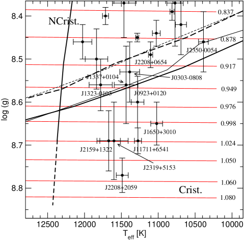
Figure 11: A zoom of Figure 5 on the region were crystallized DA white dwarf should be. The evolutionary tracks employed in our study are shown as red lines along with its value of the stellar mass. The thick full (dashed) lines indicate the limit between crystallization (Crist.) and no$-$crystallization (NCrist.) for the H2010 (SC1993) phase diagram corresponding to models with canonical H envelopes, and thin lines are for models with the thinner H envelope of each sequence.

As it is well known, the temperature at the onset of crystallization depends mainly on the stellar mass, as can be seen from Table LABEL:teff-crist, where we list the atmospheric parameters at which crystallization begins, for a given stellar mass. We only show our results for sequences with canonical hydrogen envelopes, meaning those with a $M_{\rm H}$ value obtained from full stellar evolutionary computations. As we can see, crystallization begins at a higher effective temperature for massive sequences. This comes from the fact that more massive white dwarf stars have higher central densities, and since the crystallization temperature is proportional to density ($\sim\rho^{1/3}$ for a carbon pure composition), it increases with the stellar mass. It is worth noting that the crystallization temperatures when only the release of latent heat is taken into account, are similar to those for SC1993 phase diagram. In addition to the dominant stellar mass dependence, there is a weak dependence of the crystallization effective temperature with the mass of the hydrogen envelope: thinner hydrogen envelope sequences usually begin to crystallize at slightly higher effective temperatures. For example, for a $\sim 0.998M_{\odot}$ model, the crystallization effective temperature goes from $12\,773$ K ($13\,802$ K) to $12\,930$ K ($13\,920$ K) when $M_{\rm H}$ decreases from $M_{\rm H}=1.98\times 10^{-6}M_{*}$ to $M_{\rm H}=4.96\times 10^{-10}M_{*}$, considering the H2010 (SC1993) phase diagram (see Figure 11). Also, for a given stellar mass, different crystallization phase diagrams leads to different crystallization temperatures, in agreement with the results of Horowitz et al. (2010) and Althaus et al. (2012) (see their Figure 1). In fact, the crystallization temperature predicted using the SC1993 phase diagram is $\sim 1000$ K higher than that predicted by the H2010 phase diagram. Finally, note that for sequences with a stellar mass lower than $0.878M_{\odot}$ for SC1993, and lower than $0.917M_{\odot}$ for H2010, crystallization begins at effective temperatures lower than the observational red edge of the instability strip.

From the results presented in Althaus et al. (2012), we not only expect differences in the amount of energy release, but also on the oxygen distribution in the white dwarf interior (see their Figures 2 and 3), which in turn should leave non$-$negligible imprints in the pulsation spectrum. We start by analyzing the impact of crystallization on the theoretical period spectrum. In Figure 3 we depict the evolution of the $\ell=1$ periods in terms of $T_{\rm eff}$ corresponding to sequences with stellar mass $0.998M_{\odot}$ and canonical H envelopes, for the cases when we only consider the release of latent heat as an additional energy source (left panel, LH), and when we employ the H2010 (left panel) and SC1993 (right panel) crystallization treatments. The vertical lines indicate the effective temperature at which crystallization begins (see Table LABEL:teff-crist). Note that low radial order modes, $k=1,2,3$, are almost unaffected when we include phase separation upon crystallization in our computations. On the other hand the period values for modes with radial order $k\geq 4$ begin to increase when crystallization sets in the models. This is because high radial order modes behave according to the predictions of the asymptotic theory, where the period values are given by $\Pi_{k}\propto k\times(\int_{r_{1}}^{r_{2}}|N|dr/r)^{-1}$ (Tassoul et al. 1990), while low radial order modes do not follow the asymptotic prescriptions and then are not affected by the crystallization process. In addition, the size of the propagation region becomes smaller as the crystallization front moves outwards leading to an increase in the period values. An important feature displayed in Figure 3 is that when crystallization begins the mode bumping/avoided crossing phenomena propagates to longer periods, and is reinforced in the H2010 and SC1993 cases. Since the crystallization temperature is higher for SC1993 treatment, at a given effective temperature the amount of crystallized mass should be larger when we employ this phase diagram than when we consider the H2010 phase diagram. In fact, for the $k=4$ mode and $T_{\rm eff}=11\,600$ K, the theoretical period value is 221.495 s when we only consider the release of latent heat, and 238.164 s and 244.370 s when we also take into account phase separation considering the H2010 and the SC1993 phase diagrams, respectively.

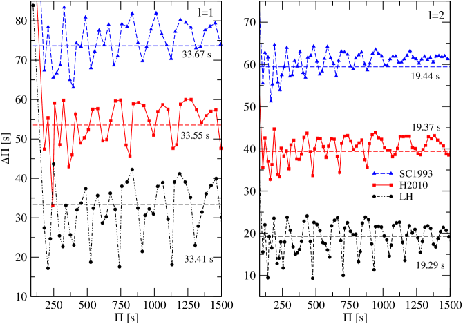
Figure 4: Theoretical period spacing in term of the periods for models with $M_{*}=0.998M_{\odot}$ and $T_{\rm eff}=11\,600$ K for modes with $\ell=1$ (left panel) and $\ell=2$ (right panel). We show our results obtained by considering only the release of latent heat (black circles) and by employing the SC1993 (blue triangles) and H2010 (red squares) phase diagrams. The value of the asymptotic period spacing (horizontal lines) is indicated in each case. The curves are shifted upwards in 20 s from the one below it, except for the bottom curve.

Finally, in Figure 4 we plot the forward period spacing in terms of the periods, for three models characterized by $M_{*}=0.998M_{\odot}$ and $T_{\rm eff}=11\,600$ K and different crystallization treatments. The left panel depicts our results for $\ell=1$ modes, while the right panel does it for the $\ell=2$ modes. Black circles depict the results in the case in wich we neglect phase separation upon crystallization and only include the release of latent heat in our computations (LH), while red squares and blue triangles depict the results when we employ the phase diagrams of Horowitz et al. (2010) and Segretain & Chabrier (1993), respectively.

As the crystallization front moves towards the surface of the model, not only the propagation region shortens but also the chemical structure of the crystallized region becomes invisible to the oscillation. This in turns will leave a signature on the periods spacing, as can be seen from Figure 4. Note that the structure of $\Delta\Pi$ has less features when phase separation upon crystallization is included in the computations. The minima in $\Delta\Pi$ are less pronounced and the departure from the asymptotic period spacing (straight horizontal line) is smaller for the H2010 and SC1993 models than for the LH model. This feature is more noticeable for $\ell=2$ modes. We also find these trends by comparing the run of the period spacing for the H2010 and SC1993 models. Since the computations using the Horowitz et al. (2010) phase diagram give a lower crystallization temperature (see Table LABEL:teff-crist), the percentage of crystallized mass is $\sim 10\%$ lower for the H2010 model than for the SC1993 model. Then the structure of the period spacing is smoother and shows less features for the SC1993 model.

In closing, note that the value of the asymptotic period spacing slightly increases with the amount of crystallized mass in the models, as predicted by Eq. 1. For $\ell=1$ modes this value goes from 33.41 s when we neglect the release of energy due to phase separation, to 33.55 s when we employ the H2010 phase diagram in our computations, and to 33.67 s when we consider the phase diagram from SC1993 instead. This increase, although small, is solely due to the change in the treatment of crystallization, since we are keeping the stellar mass and effective temperature fixed.

4 Stars analyzed and the spectroscopic mass

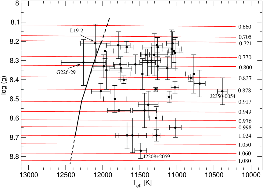
Figure 5: The location of the 42 ZZ Ceti stars analyzed in this paper in the spectroscopic $\log g-T_{\rm eff}$ plane. The thin red lines correspond to our set of DA white dwarf evolutionary tracks with thick (canonical) H envelope thickness and stellar masses ranging from 0.660$M_{\odot}$ to 1.080$M_{\odot}$. The thick line depicts the theoretical blue edge of the instability strip for massive DA white dwarf stars (see text for details).

We analyzed a set of 42 ZZ Ceti stars with spectroscopic stellar mass between 0.72$M_{\odot}$ and 1.05$M_{\odot}$. This sample belongs to the massive component of the white dwarf mass distribution presented in Kleinman et al. (2013). Note that the mass range considered for the sample corresponds to white dwarfs thought to harbor cores made of carbon and oxygen. Thus, the most massive DAV stars, like BPM 37093 ($M_{*}\sim 1.1M_{\odot}$) probably having an oxygen$-$neon core (Kanaan et al. 1998; Metcalfe et al. 2004; Kanaan et al. 2005), are not included in our current sample. The atmospheric parameters for each of these stars are listed in columns 2 and 3 of Table 3. For the first 36 objects, the atmospheric parameters were taken from Kleinman et al. (2013), based on spectra taken from the SDSS Data Release 7 (Abazajian et al. 2009). For J1916$+$3938 the $T_{\rm eff}$ and $\log g$ values were taken from Hermes et al. (2011). The last five objects are bright ZZ Ceti stars (e.g. Fontaine & Brassard 2008), four of which were already analyzed from an asteroseismological point of view in Romero et al. (2012). Since the classical ZZ Ceti stars have been targeted in several works, there are several determinations of their atmospheric parameters. Thus, within the uncertainties, the values listed in Table 3 include all the effective temperature and surface gravity determinations from the literature. The fact that the uncertainties for the stars from the SDSS are smaller that those for the classical ZZ Ceti, may indicate that these uncertainties are most probably underestimated. However, we must note that SDSS counts with better flux calibrations and also that the $T_{\rm eff}$ and $\log g$ values are determined considering all the spectrum and not only the Balmer$-$line profiles as in Bergeron et al. (2004). The location of the 42 DAV stars targeted in this work on the $\log g-T_{\rm eff}$ plane are shown in Figure 5, along with the evolutionary tracks with masses ranging from 0.660 to 1.080 $M_{\odot}$. Some objects are indicated by their denomination. In particular, the two bright ZZ Ceti stars G226-29 and L19-2, are the hottest stars in the sample. On the other hand, J2350$-$0054 is the coolest massive DA variable known to date (Mukadam et al. 2004). Finally, J2208$+$2059 shows the highest spectroscopic mass of our DAV sample (Castanheira et al. 2013b).

Evolutionary sequences characterized by stellar masses in the range of 0.660 $-$ 1.050$M_{\odot}$ correspond to carbon$-$oxygen core models (see section 2.2). The sequences with stellar mass of 1.060 and 1.080$M_{\odot}$ have an oxygen$-$neon core and were taken from Althaus et al. (2005c). The latter sequences were not considered in our asteroseismological analysis. It is important to note that all the sequences were generated with the LPCODE evolutionary code (Althaus et al. 2010b; Renedo et al. 2010).

The spectroscopic mass values (column 4 of Table 3) were estimated by a linear interpolation of the evolutionary tracks in the $\log g-T_{\rm eff}$ diagram given the values of $\log g$ and $T_{\rm eff}$ inferred from spectroscopy. The mean value for the spectroscopic mass of our sample of 42 DAV stars is $\langle M_{*}\rangle_{\rm spec}=0.841\pm 0.093M_{\odot}$. Kleinman et al. (2013) found a mean value of $\langle M_{*}\rangle=0.822M_{\odot}$ for the massive component in the mass distribution of DA white dwarf stars ($\sim 280$), including variable and non$-$variable stars but also for objects with masses above 1.050 $M_{\odot}$. Taking these differences into account, and our limited sample, the agreement between the mean mass obtained in this work and that of Kleinman et al. (2013) is excellent.

Finally, we include in Figure 5 the theoretical blue edge of the instability strip for massive DA white dwarf stars, depicted as a thick vertical line. This blue edge was obtained by means of non$-$adiabatic computations employing the non$-$adiabatic version of the LP-PUL pulsation code described in detail in Córsico et al. (2006), adopting a MLT parameter $\alpha=1.61$. Our computations rely on the frozen convection approximation, were the perturbation of the convective flux is neglected. While this approximation is known to give unrealistic locations of the $g$-mode red edge of instability, it leads to satisfactory predictions for the location of the blue edge of the ZZ Ceti (DAV) instability strip (see, e.g., Brassard & Fontaine 1999), for the V777 Her (DBV) instability strip (see, for instance, Beauchamp et al. 1999 and Córsico et al. 2009a), and also for the instability strip of low$-$mass pulsating DAV stars (Córsico et al. 2012c). In addition, the stability computations employing the time$-$dependent convection treatment show that the theoretical blue and red edges are not dramatically different from the ones found by applying the frozen convection approximation (Van Grootel et al. 2012; Saio 2013). The location of the theoretical blue edge of the instability strip is strongly dependent of the convective efficiency adopted in the envelope of the stellar models. Then the location of the blue edge can be hotter (cooler) if we adopt a larger (smaller) value for the mixing length parameter $\alpha$. From Figure 5 we find that the location of the theoretical blue edge agrees with the observations since most of the DAV stars are predicted to be pulsationally unstable. Although L19$-$2 and G226$-$29 are found to be hotter than our theoretical blue edge, within the uncertainties these objects are also inside the theoretical instability strip.

5 New Observations

As part of an ongoing program devoted to observe known DA variable white dwarfs, in order to increase the number of detected modes, and find new variable ZZ Ceti stars, we re-observed some of the objects from our sample of massive DAV stars. Here we present new observations for five targets, obtained at different campaigns from 2010 to 2013. All targets were observed with the Soar Optical Imager and the Goodman High Throughput Spectrograph on the 4.1 m SOAR telescope, in Chile. For details on the instruments used and the data reduction see e.g Castanheira et al. (2010). We present a journal of observations in Table 4.

6 Results: Asteroseismological fits

For each massive ZZ Ceti star listed in Table 3, we search for an asteroseismological representative model, that best matches the observed periods. To this end, we seek for the theoretical model that minimize the quality function given by Bradley (1998):

$$\Phi(M_{*},M_{\rm H},T_{\rm eff})=\frac{1}{N}\sum_{i=1}^{N}{\rm min}\left|\Pi_{k}^{\rm th}-\Pi_{i}^{\rm obs}\right|,$$ (2)

where $N$ is the number of periods observed in the target star. Since the period spacing for $\ell=2$ is smaller than that for $\ell=1$ modes, there are always more quadrupolar modes for a given model when we consider a fixed period interval. So, we require them to be closer to the observed period by a factor of $N_{\ell=2}/N_{\ell=1}$ in order to be chosen as a better match (Metcalfe et al. 2004).

We also considered the quality functions given by Córsico et al. (2009b):

$$\chi^{2}(M_{*},M_{\rm H},T_{\rm eff})=\frac{1}{N}\sum_{i=1}^{N}{\rm min}\left[\Pi_{k}^{th}-\Pi_{k}^{obs}\right]^{2},$$ (3)

and the quality function employed in Castanheira & Kepler (2008):

$$\Xi(M_{*},M_{\rm H},T_{\rm eff})=\sum_{i=1}^{N}\sqrt{\frac{\left[\Pi_{k}^{th}-\Pi_{k}^{obs}\right]^{2}A_{i}}{\sum_{i=1}^{N}A_{i}}},$$ (4)

where the observed amplitudes $A_{i}$ are used as weights for each period. In this way, the period fit is more influenced by those modes with large observed amplitudes. Since the three quality functions usually leads to similar results, we shall describe the quality of our period fits in terms of the function $\Phi(M_{*},M_{\rm H},T_{\rm eff})$ only.

The results from our asteroseismological study are presented in Tables Asteroseismological study of massive ZZ Ceti stars with fully evolutionary models and 6. In Table Asteroseismological study of massive ZZ Ceti stars with fully evolutionary models we list the results for the 18 stars showing three or more periods in their observed spectrum, while for those stars having one or two observed periods the results are presented in Table 6. Both tables are organized as follows. In the second, third and fourth columns, we show the values of the effective temperature, stellar mass and thickness of the hydrogen envelope for a given asteroseismological model. Columns 5 and 6 show the observed periods and amplitudes corresponding to each star, extracted from different works listed in column 12. The theoretical periods, along with the corresponding harmonic degree and radial order, are listed in columns 7, 8 and 9, respectively. The value of the quality function $\Phi(T_{\rm eff},M_{*},M_{\rm H})$ for each asteroseismological model is listed in column 10. In column 11 we list, whenever appropriate, the phase diagram considered in the treatment of crystallization and the fraction of the crystallized mass. For several objects we show more than one asteroseismological solution. The first model listed is the one we choose to be the best fit model for that particular object, and refer to the remaining solutions as the second and third solution, whenever it is the case.

In Table LABEL:tabla-sismology we list the structural parameters of the astroseismological models selected as best fit models for each star analyzed in this paper. The uncertainties for $M_{*}$, $T_{\rm eff}$, and $\log(L/L_{\odot})$ were computed by employing the following expression (Zhang, Robinson & Nather 1986; Castanheira & Kepler 2008)

$$\sigma^{2}_{i}=\frac{d_{i}^{2}}{(S-S_{O})},$$ (5)

where $S_{0}\equiv\Phi(M_{*}^{0},M_{\rm H}^{0},T_{\rm eff}^{0})$ is the minima of the quality function $\Phi$ reached at $(M_{*}^{0},M_{\rm H}^{0},T_{\rm eff}^{0})$ corresponding to the best fit model, and $S$ is the value of $\Phi$ when we change the parameter $i$ by an amount $d_{i}$, keeping fixed the other parameters. The quantity $d_{i}$ can be evaluated as the minimum step in the grid of parameter $i$. The uncertainties in the other quantities are derived from the uncertainties in $M_{*}$, $T_{\rm eff}$, and $\log(L/L_{\odot})$. These uncertainties represent the internal errors of the fitting procedure. Other uncertainties come from the modeling itself. For example, the treatment of extra$-$mixing process depends on a free parameter $f$, that can vary at different stages of the evolution, and also will depend on the chemical composition of the convective region (see sec. 2.1). Also, the final carbon and oxygen central abundances depend on the value of the ${}^{12}C(\alpha,\gamma)O^{16}$ reaction rate, which cannot be estimated experimentally, leading to uncertainties on the final composition of the white dwarfs core. Finally, mass loss episodes depend on several parameters, including the metallicity, the amount of helium and rotation. Unfortunately a value for these uncertainties is not easy to asses.

Because most of the stars in our sample of 42 DAVs show only a few periods, we can not rely only on the observed periods to select a single asteroseismological model, among all the possible and equally valid solutions, and we must apply some criteria. They are:

• First we looked for those models associated to minima in the quality function, to ensure that the theoretical periods are the closest match to the observed values.

• When we found several families of solutions with similar values of the quality function, we choose those models with values of $T_{\rm eff}$ and $\log g$ as close as possible to the spectroscopic values. In particular, we consider that the spectroscopic determination of the effective temperature is more accurate than that of the surface gravity, so we give more weight to the spectroscopic value of $T_{\rm eff}$, as we will discuss in the next section.

• When possible, we used the external identification of $\ell$ values for the observed periods, mainly inferred from splitting due to the presence of rotation and/or magnetic fields, even if not all the components of the multiplet reach observable amplitudes.

• When two or more modes have similar observed amplitudes in the power spectrum, we gave more weight to stellar models that fit those periods with theoretical periods having the same harmonic degree $\ell$.

• We give more weight to solutions that fit the largest amplitude modes with theoretical modes having $\ell=1$, since dipolar modes would exhibit larger amplitudes than $\ell=2$ modes, because geometric cancellations effects become more important for modes with higher harmonic degree (Dziembowski 1977; Robinson, Kepler & Nather 1982). However, for white dwarf stars having a large fraction of its mass in a crystallized state, the possible propagation region for $g-$modes is quite small, since oscillations cannot propagate in the crystallized regions of the star. In this context, quadrupolar modes may be favored to be excited to observable amplitudes since they have shorter wavelengths. Thus, this restriction can not be applied in these cases.

6.1 Particular cases

Next, we briefly summarize some details related to the asteroseismological analysis for a few cases of interest.

J0048$+$1521: This star shows two modes with very close periods at 615.3 and 604.19 s with similar amplitudes. In this case, the period spacing will be of $\sim 11.11$ s only compatible with modes trapped in the outer layers (Althaus et al. 2010b) or with unrealistic massive white dwarf (Nityananda & Konar 2013; Das et al. 2013). We assume that these two modes are the $m=\pm 1$ components of a $\ell=1$ rotation triplet in which the central component is absent from the pulsation spectrum. For our asteroseismological fit we consider a period at 609.75 s, corresponding to the $m=0$ component computed as the average value between the two observed components. By assuming rigid slow rotation we infer a mean rotation period of $\sim 9$ h, in line with the values derived for other ZZ Ceti stars from asteroseismology (see, for instance, Table 4 of Fontaine & Brassard 2008).

J0923$+$0120: Variability in J0923$+$0120 was reported by Mukadam et al. (2004), with one observed period at $\sim 595$ s. Further observations performed during 2006 in the McDonald Observatory, Apache Point, BOAO (Korea) and HCT in India (A. Mukadam, private communication) reveled three additional very long periods at 4145.0, 2032.3 and 1436.37 s. The longest period was dismissed since it is most likely to be low frequency noise. Surprisingly, no modes with periods between 600 and 1400 s were found. In our asteroseismological study we consider only two periods, 595.055 and 1436.37 s. Because the theoretical periods computed in this work reaches a longest value of $\sim$ 2000 s, the period at 2032.30 s was not included in our analysis.

J1323$+$0103: This star shows the most populated period spectrum of our sample, with 15 periods considered in our seismological fit. The periods listed in Table Asteroseismological study of massive ZZ Ceti stars with fully evolutionary models, are a combination of two sets of observations. The first set corresponds to those periods reported by Kepler et al. (2012), who performed asteroseismological fits employing the model grid presented in Romero et al. (2012) and Castanheira & Kepler (2008). The results from seismology by using the full evolutionary models following Romero et al. (2012) are: $M_{*}=0.88\pm 0.02M_{\odot}$, $T_{\rm eff}=12\,100\pm 140$ K, $M_{\rm H}=(4.0\pm 3.3)\times 10^{-7}M_{*}$, $M_{\rm He}=(2.6\pm 0.3)\times 10^{-3}M_{*}$, $X_{\rm C}=0.37\pm 0.01$ and $X_{\rm O}=0.62\pm 0.01$. The results obtained by employing the models described in Castanheira & Kepler (2008), which assume a central composition C/O = 50% and allow the hydrogen and helium layer mass to vary, are: $T_{\rm eff}=11\,900\pm 200$ K, $M_{*}=0.88\pm 0.08M_{\odot}$, $M_{\rm H}=10^{-4.5\pm 0.4}M_{*}$ and $M_{\rm He}=10^{-2.3\pm 0.5}M_{*}$. The large difference in the hydrogen content of the two seismological fits can be interpreted in terms of the core$-$envelope symmetry (Montgomery et al. 2003) and the differences in the chemical structures characterizing both model grids.

A second set of periods was obtained from observations performed at the SOuthern Astrophysical Research telescope (SOAR) in 2012 (see Sec. 5). Although some modes were already present in the first set, most of the observed modes in the second set have not been observed before. In our asteroseismological study we consider both set of observed periods, using an average value for those periods present in both sets. We obtain a best fit model characterized by $M_{*}=0.917\pm 0.020M_{\odot}$, $T_{\rm eff}=11\,535\pm 72$ K, $M_{\rm H}=3.90\times 10^{-6}M_{*}$, $M_{\rm He}=1.31\times 10^{-3}M_{*}$ and $X_{\rm O}=0.609$. The stellar mass is a bit higher than that obtained in the previous seismological study, but compatible with the spectroscopic determinations. On the other hand, the mass of the hydrogen layer is about one order of magnitude thicker than that obtained by employing the models from Romero et al. (2012), but still thin as compared with the solution obtained using the models of Castanheira & Kepler (2008).

J1612$+$0830: This star was reported to be variable by Castanheira et al. (2013a), with two very close observed periods, 115.17 and 117.21 s, and very similar observed amplitudes. A close inspection of the Fourier transform (see Figure 1 of Castanheira et al. 2013a) shows the presence of a low amplitude third peak at $\sim 112$ s. Therefore, the three observed periods are the components of a rotational $\ell=1$ triplet, being the central component at 115 s. We employ the two main components at 115 s and 117 s to derive a mean rotation period of $\sim 1$ h, considering slow rigid rotation. Note that J1612$+$0830 shows a $\ell=1$ triplet with very short periods, similar to G226$-$29. Also the seismological solutions obtained for both stars are very similar, with a thick hydrogen envelope and effective temperatures close to the blue edge. However, the rotation period derived for G226$-$29 is $\sim 9$ h (Kepler et al. 1995).

J1711$+$6541: As J0048$+$1521, this star shows two modes with very close periods at 612.6 and 606.3 s and similar amplitudes. We assume that these modes are the $m=\pm 1$ components of a $\ell=1$ rotation triplet, with a not observed $m=0$ component at 609.45 s. Considering rigid, slow rotation we derive a mean rotation period of $\sim 16.4$ h.

J2128$-$0007: Although the spectroscopic mass for J2128$-$0007 is close to the lower limit of our sample, $\sim 0.788M_{\odot}$, we obtain a seismological solution with a stellar mass of 0.976$M_{\odot}$. The second solution with $\sim 0.593M_{\odot}$ listed in Table Asteroseismological study of massive ZZ Ceti stars with fully evolutionary models is probably related to the presence of the two modes with periods at $\sim$ 274 s and $\sim$ 304 s, since they are close to the modes observed in G117$-$B15A at 270.46 s and 304.05 s (Kepler et al. 1982). Romero et al. (2012) found a seismological solution for G117$-$B15A with the same stellar mass, and a thin H envelope ($M_{\rm H}=1.25\times 10^{-6}M_{*}$). For J2128$-$0007 we obtain a solution with thick hydrogen envelope, since for G117$-$B15A this parameter is basically set by the mode at $\sim$ 215 s (see Romero et al. 2012 for details).

J1916$+$3938: This star is the first pulsating DA white dwarf star located in the Kepler mission field (Kepler ID 4552982) and identified through ground$-$base time series photometry by Hermes et al. (2011). As a result, these authors found seven possible modes that are listed in Table 5. The first seismological study applied to this object was performed by Córsico et al. (2013b) employing the model grid presented in Romero et al. (2012). In this work we reanalyze this star and obtain the same asteroseismological model. Note that the two shortest modes, with periods at 823.9 and 834.1 s are associated with theoretical modes showing different harmonic degrees. Other possibility is that these two modes are the $m=\pm 1$ components of a rotational triplet in which the central component is not present. The period of the missing $m=0$ component can be estimated as the average of the $m=\pm 1$ components, at 829 s. Under this assumption, we performed an asteroseismological fit replacing the two shortest periods by their average. As a result we obtained the same asteroseismological solution as before. Finally, by assuming rigid and slow rotation we can infer a mean rotation period of 18.77 h.

The classical ZZ Cetis: G226$-$29, L19$-$9, G207$-$9 and BPM 30551: of our sample of 42 massive DAV stars, four of them were also part of the sample studied by Romero et al. (2012). Since now we have available an expanded grid, and the additional parameter given by the crystallization treatment, we think it is worthwhile to reanalyze these objects. The observed periods and amplitudes are the same as in Romero et al. (2012), except for L19$-$2 that was re-observed (see Sec. 5). The asteroseismological models obtained for G226$-$29 and G207$-$9 are the same as those presented in Romero et al. (2012). For BPM 30551 we obtain a best fit model with $M_{*}=0.721M_{\odot}$ and $T_{\rm eff}=11\,157$ K and $\Phi=0.176$ s, in addition to a second solution with $M_{*}=0.705M_{\odot}$ and $T_{\rm eff}=11\,436$ K and $\Phi=0.175$ s, that corresponds to the seismological solution found in Romero et al. (2012) for this star. We select the seismological model with $M_{*}=0.721M_{\odot}$ over the model with $M_{*}=0.705M_{\odot}$ because the effective temperature and stellar mass are in best agreement with the spectroscopic values. Finally, for L19-2 we found a seismological solution corresponding to the same evolutionary sequence than the solution presented in Romero et al. (2012) but $\sim 70$ K cooler.

6.2 Very cool massive ZZ Ceti or low mass variable white dwarfs?

From our sample of 42 DAV stars, we focus here on three of them: J0000$-$0046 reported by Castanheira et al. (2006), J0940$+$0052 discovered by Castanheira et al. (2013a) and J2350$+$0054 reported by Mukadam et al. (2004). From spectroscopy, these stars show very low effective temperatures and high surface gravities, being J2350+0054 the most extreme, with $T_{\rm eff}=10\,387\pm 66$ K and $\log g=8.46\pm 0.07$. Since these stars are located near the red edge of the instability strip, they should have a period spectrum characterized by several modes with long periods (Mukadam et al. 2006). However, the three objects show only a few modes with short periods in their observed spectrum, characteristic of DAV stars near the blue edge of the instability strip. This is particularly true for J0940$+$0052 and J2350$+$0054 that show a few modes with periods between 250 and 400 s. Here, we consider two possible simple explanations: (1) the spectroscopic determination of the effective temperature is not correct and these stars are hotter than predicted, or (2) the surface gravity values are not correct and these stars are not massive white dwarfs but low mass white dwarf stars, that are also known to be variable (Hermes et al. 2012, 2013a). Since usually the $\log g$ value is the one that is most poorly determined from spectroscopy, as we discuss in Section 6.3, we consider the second possibility as the most likely. For low mass variable white dwarfs the blue edge of the instability strip is located at considerably lower effective temperatures than for the classical ZZ Ceti stars, as shown in Córsico et al. (2012c). In fact, if we consider the values of $T_{\rm eff}$ for J0000$-$0046, J0940$+$0052 and J2350+0054, we find that they are compatible with stars located close to the low mass stars blue edge, with stellar masses $\mathrel{\hbox{\hbox to0.0pt{\hbox{\lower 4.0pt\hbox{$\sim$}}\hss}\hbox{$>$}}}0.4M_{\odot}$ for the first two objects, and $\mathrel{\hbox{\hbox to0.0pt{\hbox{\lower 4.0pt\hbox{$\sim$}}\hss}\hbox{$>$}}}0.3M_{\odot}$ for J2350$+$0054. Further analysis on these objects needs to be done, both from the observational as well as from the asteroseismological point of view, but with more modes detected.

6.3 Stellar mass from asteroseismology

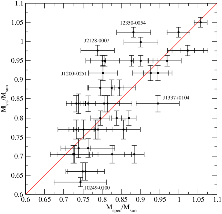
Figure 6: Comparison between the values of the stellar mass according to spectroscopy and asteroseismology. The uncertainties in the asteroseismological mass are the internal uncertainties of the fitting procedure. The red line represents the 1:1 correspondence.

In this section we compare the results obtained for the stellar mass from spectroscopy and seismology for our sample of 42 DAV stars. Since the evolutionary models employed to obtain a seismological representative model for each object are the same we use to derive the spectroscopic mass from the observed atmospheric parameters, this comparison is worth doing. In Figure 6 we compare both determinations of the stellar mass. The red diagonal line shows the 1:1 correspondence. As we can see from this figure, the agreement between both determination is not very good, reaching discrepancies as high as $\sim 0.2M_{\odot}$ for J2128$-$0007 and J1200$-$0251, $\sim 0.14M_{\odot}$ for J2350$-$0054 and around $\sim 0.1M_{\odot}$ for J1337+0104. On the other hand the bulk of the points does cluster around the 1:1 correspondence line, implicating that no significant offset is present between the asteroseismological and spectroscopic determinations of the stellar mass.

There are some shortcomings that can lead to erroneous determination of the observational parameters and thus affect further determinations of the stellar mass from spectroscopic data as well as from asteroseismology. As it is well known, determination of the surface gravity for cool DA white dwarf stars with effective temperatures $\mathrel{\hbox{\hbox to0.0pt{\hbox{\lower 4.0pt\hbox{$\sim$}}\hss}\hbox{$<$}}}12\,500$ K leads to higher values of $\log g$ than those of hotter stars. First it was thought that the presence of helium from convective mixing could mimic the effects of high surface gravities (Bergeron et al. 1991). However, this possibility was ruled out by Tremblay et al. (2010) who analyzed the high S/N spectrum of six DA white dwarfs with effective temperatures between $\sim 12\,500$ K and $\sim 10\,500$ K, and found no traces of helium. The most popular alternative explanation is related to the treatment of convective energy transport, which is currently represented by the mixing length theory in 1D models (Tremblay et al. 2010; Koester et al. 2009). In addition, Tremblay et al. (2011, 2013) show that 3D model spectra provide a much better characterization of the mass distribution of white dwarfs and the shortcomings in the 1D mixing length theory was in fact producing the high$-\log g$ problem.

Also, the presence of a magnetic fields can mimic the line broadening produced by a high surface gravity in the observed spectrum when the resolution in wavelength is not good enough to resolve the different components of the splitting, leading to an incorrect (higher) $\log g$ determination (Kepler et al. 2013). On the other hand, the presence of a magnetic field can inhibit the development of certain modes, and/or its components, if the displacement direction of the moving material is perpendicular to the magnetic field (Arras 2006). Therefore some normal modes could not be present in the observed pulsation spectrum of the star.

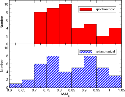
Figure 7: Histograms depicting the mass distribution for the sample of 42 ZZ Ceti massive stars with carbon$-$oxygen core, studied in this work, according to our spectroscopic (upper panel) and seismological (lower panel) analysis.

Figure 7 shows the mass distribution for the 42 massive ZZ Ceti stars analyzed in our work, according to spectroscopy (upper panel) and asteroseismology (lower panel). The spectroscopic mass distribution has its main contribution from the low mass range, for stellar masses below $0.85M_{\odot}$. On the other hand, the sesimological mass distribution shows two components, between $0.75-0.8M_{\odot}$ and $0.9-0.95M_{\odot}$. This could be due to the specific values of stellar mass in our model grid. The mean value of the asteroseismological mass is $\langle M_{*}\rangle_{\rm seis}=0.850\pm 0.110M_{\odot}$, slightly larger than the spectroscopic value $\langle M_{*}\rangle_{\rm spec}=0.841\pm 0.093M_{\odot}$. Note that the methods employed to derive both values of the stellar mass are quite different. Also, they rely on two different independent sets of observational data, being the spectrum for the spectroscopic mass, and the observed periods in the case of the seismological determinations. Taking this fact into account, the agreement between the spectroscopic and the seismological mean mass is satisfactory.

6.4 Effective temperature from asteroseismology

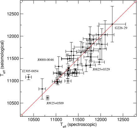
Figure 8: Comparison between the spectroscopic ($x$ axis) and seismological ($y$ axis) determination of effective temperature for our sample of 42 DAV stars. The red line indicates the 1:1 correspondence.

In Figure 8 we compare the spectroscopic ($x-$axis) and asteroseismological ($y-$axis) determinations for the effective temperature. Error bars in the asteroseismological values depict the internal uncertainties from the fitting procedure, while the uncertainties in the spectroscopic determination are the spectroscopic fitting uncertainties (see Table 3). The diagonal red line shows the 1:1 correspondence. As can be seen from this figure the correspondence between both determinations is quite good, specially in the high effective temperature domain. The larger discrepancies appear to be located at low effective temperatures. In particular, for J2305$-$0054, and J0000$-$0046, the seismological effective temperature is $\sim 700$ K and $\sim 580$ K higher than the spectroscopic value, respectively. Large discrepancies at low temperatures are expected since the atmosphere models employed to fit the observed spectra use the MLT theory of convection. The MLT theory is a good approximation for stars near the blue edge of the instability strip because the outer convective zone is still very thin. However, for lower effective temperatures closer to the red edge of the instability strip the outer convection region is quite thick, and the shortcomings from applying the MLT might be important. In addition, the convective properties do change considerably in the effective temperature range $13\,000-6\,000$ K, as is seen from 3D model atmosphere computations (Tremblay et al. 2013).

As we mention, one of the criteria applied to elect a seismological model as a possible solution is set by the atmospheric parameters determined from spectroscopy. In particular, we give more weight to the effective temperature determination than the $\log g$, therefore our seismological solutions tend to have a better agreement with the spectroscopic effective temperatures than with the spectroscopic stellar masses, as can be seen from Figures 6 and 8. If we gave more weight to the spectroscopic surface gravity, the differences between the spectroscopic and seismological values of $T_{\rm eff}$ would be as large as $\sim 500$ K for $T_{\rm eff}\mathrel{\hbox{\hbox to0.0pt{\hbox{\lower 4.0pt\hbox{$\sim$}}\hss}\hbox{$>$}}}11\,000$K.

6.5 The thicknesses of the Hydrogen envelope

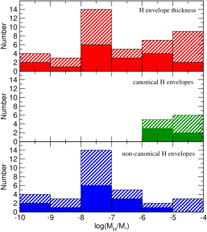
Figure 9: Upper panel: histogram showing the hydrogen envelope thickness distribution for our complete sample of 42 massive DAV stars (dashed). Middle panel: histogram for models with canonical values of the hydrogen envelope thickness, as predicted by stellar evolution theory for each mass. Lower panel: histogram for models with non$-$canonical values of the hydrogen envelope thickness, as obtained by means of our artificial procedure described in Section 2.2. We only consider the best fit model solutions for each star. In adition, with fill bars, we show the results corresponding to a sample composed only with stars having three or more modes in their spectrum (see Table Asteroseismological study of massive ZZ Ceti stars with fully evolutionary models).

Although there is some observational evidence of the existence of a range in the thickness of the hydrogen envelope, currently the hydrogen content can be determined only by asteroseismology. Since we analyze a large number of DAV stars, we can shed some light over the distribution of the hydrogen envelope mass. In the upper panel of Figure 9 we present our results for the 42 stars analyzed in this work (dashed bars). We only show the best fit model for each object. The distribution shows two maximums: for thick hydrogen envelopes, in the $\log(M_{\rm H}/M_{*})$ range $-$5 to $-$4, and for thin values in the range $-$7 to $-$8. In the middle panel of Figure 9 we show the histogram corresponding to the asteroseismological models having canonical envelopes, that amount to 10 stars. Note that the maximum amounts of hydrogen as predicted by canonical evolutionary computations, which depends on the stellar mass value, are in the range $-$4 to $-$6 for stellar masses considered in our grid. Then, the peak for thick envelopes is mostly composed by models with canonical envelopes. Finally, in the lower panel of the figure we present the histogram for the seismological models showing a non$-$canonical envelope thickness, that is, envelopes thinner than those predicted by our standard stellar evolution models. We recall that these thinner envelopes where generated via an artificial procedure described in Section 2.2 in order to extend the exploration of the parameter space of the models for asteroseismology. As it is expected, the second peak in the distribution in the range $-$7 to $-$8 is completely composed by models with non$-$canonical hydrogen envelopes, that amount to 14 objects. Also, it appears to exist a much less notorious third peak in the distribution for very thin envelopes in the range $-$10 to $-$9. The envelope distribution for a reduced sample, composed by the objects showing three or more observed modes (see Table Asteroseismological study of massive ZZ Ceti stars with fully evolutionary models), is depicted in Figure 9 with filled symbol. As can be seen from this figure, the envelope distribution has a similar shape when compared with the distribution for the full sample. There is a dominant peak in the range $-7$ to $-$8 and a weaker contribution from very thin envelopes in the range $-9$ to $-$10, both composed by non$-$canonical envelopes. In addition, five out of six seismological models with hydrogen envelopes in the range $-$4 to $-$6 correspond to canonical models. In this case, 72 % of the seismological models have non$-$canonical envelopes. Romero et al. (2012), using a different sample of DAV stars characterized with stellar masses around $0.6M_{\odot}$, also found a peak in the hydrogen envelope distribution corresponding to very thin envelopes (see their Figure 11), apart from the dominant component in the range $-$4 to $-$5. The hydrogen envelope distribution presented in that work does not show a thin component in the range $-$7 to $-$8. Finally, note that most of the seismological models obtained in our study, $\sim 76\%$, have non$-$canonical envelopes.

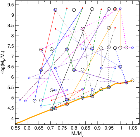
Figure 10: The values of the hydrogen envelope mass in terms of the stellar mass corresponding to all the asteroseismological models of the 42 massive ZZ Ceti stars studied in this work. Large black, medium blue and little full red circles correspond to the first, second and third asteroseismological solution, respectively, for each star (see Tables Asteroseismological study of massive ZZ Ceti stars with fully evolutionary models and 6). Solutions corresponding to the same object are joined together. The thick orange line depicts the canonical values of the hydrogen envelope thickness (color version of this figure is only available in the on-line version).

In Figure 10 we plot the thickness of the hydrogen envelope in terms of the stellar mass for the asteroseismological models listed in Tables Asteroseismological study of massive ZZ Ceti stars with fully evolutionary models and 6. With black large circles we plot the best fit models for each star, whereas blue medium and small full red circles represent the second and third solutions, when present. Solutions corresponding to the same object are joint together with a line. The gray thick line indicates the high limit of the hydrogen mass, as predicted by stellar evolution. Note that for several objects, we obtain two possible seismological solutions, one characterized by a high stellar mass and a thin hydrogen envelope and other characterized by a lower mass and a thicker hydrogen layer. For example, for J2128$-$0007 we obtained a best fit model characterized by $M_{*}=0.976M_{\odot}$ and $\log(M_{\rm H}/M_{*})=-9.29$ and a second solution with $M_{*}=0.593M_{\odot}$ and $\log(M_{\rm H}/M_{*})=-4.85$. This degeneracy in solutions is related to the so called “core $-$ envelope symmetry” discussed in Montgomery et al. (2003), where a sharp feature in the Brunt$-$Väisälä frequency in the envelope can produce the same period changes as a bump placed in the core.

The mean value of the hydrogen layer mass is $\langle M_{\rm H}/M_{*})=5.24\times 10^{-6}$ for our sample of 42 massive DAV stars, and $\langle M_{\rm H}/M_{*})=4.54\times 10^{-6}$ if we consider the reduced sample of 18 stars listed in Table Asteroseismological study of massive ZZ Ceti stars with fully evolutionary models. These values are about 4 times lower than the mean value obtained by Romero et al. (2012), with a different sample of stars but the same model grid, and about 10 times larger than that from Castanheira & Kepler (2009), with a sample with a broad range in stellar mass, including very massive ZZ Ceti stars, and employing different models. Notwithstanding these differences, our results agree with those obtained by Castanheira & Kepler (2009) and Romero et al. (2012) in that the possible values of the hydrogen mass are not around $10^{-4}M_{*}$ but span over a large range ($10^{.4}-10^{-10}M_{*}$) and that an important fraction of DA white dwarf stars might be formed with an hydrogen envelope much thinner than that predicted by standard evolutionary theory. This result should have a strong impact on the derived ages from white dwarf cooling sequences for globular clusters, since it is always assumed that the amount of hydrogen in the envelope is $\sim 10^{-4}M_{*}$.

As we mentioned earlier, there are observational evidence for the existence of a range in the hydrogen layer mass. Tremblay & Bergeron (2008) determined the ratio of helium to hydrogen atmosphere white dwarf stars in terms of $T_{\rm eff}$ from a model atmosphere analysis of the infrared photometric data from the Two Micron All Sky Survey combined with available visual magnitudes. These authors found that the He/H atmosphere ratio increases gradually from $\sim 0.25$ for $15\,000K\mathrel{\hbox{\hbox to0.0pt{\hbox{\lower 4.0pt\hbox{$\sim$}}\hss}\hbox{$>$}}}T_{\rm eff}\mathrel{\hbox{\hbox to0.0pt{\hbox{\lower 4.0pt\hbox{$\sim$}}\hss}\hbox{$>$}}}10\,000K$ to $\sim 0.50$ for $10\,000K\mathrel{\hbox{\hbox to0.0pt{\hbox{\lower 4.0pt\hbox{$\sim$}}\hss}\hbox{$>$}}}T_{\rm eff}\mathrel{\hbox{\hbox to0.0pt{\hbox{\lower 4.0pt\hbox{$\sim$}}\hss}\hbox{$>$}}}8\,000K$, due to convective mixing when the bottom of the hydrogen convection zone reaches the underlying convective He envelope. They conclude that about 15% of the DA white dwarf should have hydrogen mass layers in the range $\log(M_{\rm H}/M_{*})=-10$ to $-8$. Romero et al. (2012), based on a set of 44 bright ZZ Ceti stars with stellar mass $\sim 0.6M_{\odot}$, found that $\sim 11\%$ of the sample have a thin hydrogen envelope mass in the range $10^{-10}\mathrel{\hbox{\hbox to0.0pt{\hbox{\lower 4.0pt\hbox{$\sim$}}\hss}\hbox{$<$}}}M_{\rm H}/M_{\odot}\mathrel{\hbox{\hbox to0.0pt{\hbox{\lower 4.0pt\hbox{$\sim$}}\hss}\hbox{$<$}}}10^{-8}$. From our asteroseismological results, we found that 7 out of 42 objects in our sample, $\sim 17\%$, have thin hydrogen envelopes in this range, compatible with the predictions of Tremblay & Bergeron (2008).

Recently, Kurtz et al. (2013) reported the discovery of a new class of pulsating white dwarf star, the “hot DAV” stars, characterized by hydrogen atmospheres and effective temperatures in the cooler edge of the “DB gap”, located between $45\,000-30\,000$ K. The pulsational instability of the “hot DAV” white dwarfs was predicted by Shibahashi (2005, 2007). This author found that in models with thin hydrogen envelopes and temperatures around $30\,000$ K, the radiative heat exchange leads to an asymmetry in $g-$mode oscillatory motion such that the oscillating elements overshoot their equilibrium positions with increasing velocity (Kurtz et al. 2008). He predicted that high harmonic degree $g$-modes should be excited in DA stars at the cool edge of the DB gap. Since the existence of these objects in the DB gap requires that a fraction of the “hot DAV” stars to have a thin layer of hydrogen of $\sim 10^{-12}M_{\odot}$ on top of a much thicker helium layer, the discovery of the “hot DAV” stars is a confirmation of the existence of extremely thin hydrogen envelope DA white dwarf stars.

From our set of evolutionary sequences we found that the thickness of the hydrogen envelope decreases as the stars evolves towards lower effective temperatures, until it reaches a stable value. For sequences with hydrogen layer mass below $\log(M_{\rm H}/M_{*})\sim-8$, this usually happens before the star reaches the cold end of the DB gap, so the thickness of the hydrogen layer at $30\,000$ is practically the same than that in the instability strip. Therefore, the observed ZZ Cetis must have hydrogen envelopes thicker than $\sim 10^{-12}M_{*}$ in order to remain DA white dwarfs when they reach the DA instability strip. Additional computations performed for this work show that, for a sequence with $0.593M_{\odot}$ and an hydrogen envelope mass of $1.38\times 10^{-10}M_{*}$, the outer hydrogen convective zone reaches the helium rich layer underneath for effective temperatures around $\sim 9300$ K, mixing the hydrogen with the much more abundant helium so the star becomes a DB white dwarf.

6.6 Crystallization from asteroseismology

In Figure 11 we show a zoom of the high $\log g$ region of the $T_{\rm eff}-\log g$ plane from Figure 5. Diagonal lines show the limit between crystallization (Crist.) and no$-$crystallization (NCrist.) considering the phase diagrams from H2010 (solid) and SC1993 (dashed). Thick lines correspond to sequences with canonical hydrogen envelope (see Table LABEL:teff-crist), while thin lines depict the onset of crystallization for sequences with the thinnest hydrogen envelope of the grid, for each stellar mass. According to the spectroscopic values of $T_{\rm eff}$ and $\log g$, there are $\sim 11$ objects in our sample that should have a fraction of its mass in a crystallized state according to the SC1993 phase diagram, and 6 of them according to H2010 phase diagram. These number increase if we consider the error bars. Note that the crystallized mass fraction for a given object will differ, depending on which phase diagram we are employing in our computations, being usually $\sim 10\%$ lower for H2010. It is worth noting that the crystallization temperatures when only the release of latent heat is taken into account, are similar to those for SC1993 phase diagram.

Our asteroseismological results, listed in Tables Asteroseismological study of massive ZZ Ceti stars with fully evolutionary models and 6, show that 15 out of the 42 massive DAV stars analyzed in this work have best fit models corresponding to a sequence computed by considering the release of gravitational energy due to phase separation upon crystallization, and consequently showing some fraction of its mass in a crystallized state. For nine of them, the best fit model corresponds to a sequence computed by using the H2010 phase diagram, while for the remaining six stars we obtain a best fit model corresponding to sequences where we consider the SC1993 phase diagram. Note that from the 15 stars with crystallized models, nine also show three or more observed periods (see Table Asteroseismological study of massive ZZ Ceti stars with fully evolutionary models), six of them with seismological solutions corresponding to sequences computed using the H2010 phase diagram and three with the SC1993 phase diagram. Therefore, our results from asteroseismology suggest that the Horowitz et al. (2010) phase diagram should be the most accurate representation of the crystallization process inside white dwarf stars. We must admit that in most cases we present more than one possible solution for a single object, with quality functions values that are quite close in some cases. In addition, most of the stars analyzed in this work show only a few, and sometimes one, modes in their observed spectrum, that limits the information that can be extracted from asteroseismology. However, in spite of these, we must recall that a set of rigorous criteria is applied in order to select for each star in our sample the asteroseismological model that better matches not only the observed periods but also the spectroscopic parameters and any additional observational data. In this sense we consider that our results are robust, although it should be necessary to analyze a large number of objects to place our finding on a more firmer basis.

Finally, note that the carbon$-$oxygen abundances are not considered as free parameters in our model grid. Instead, the chemical abundances of the central regions are basically given by the evolution during the central helium burning stage, where we use the ¹²C($\alpha,\gamma$)¹⁶O reaction rate given by Angulo et al. (1999) in our computations. However, we must recall that the specific value of the ¹²C($\alpha,\gamma$)¹⁶O reaction rate is still one of the current uncertainties in the theory of stellar evolution. A higher ¹²C($\alpha,\gamma$)¹⁶O reaction rate will translate into a higher oxygen abundance, increasing the crystallization temperature of the model. Our additional computations show that if we increase by a factor of 1.4 the ¹²C($\alpha,\gamma$)¹⁶O reaction rate from Angulo et al. (1999) the amount of oxygen left in a $0.998M_{\odot}$ white dwarf model will increase by $\sim 14.5\%$, and the crystallization temperature given by the phase diagram presented by Horowitz et al. (2010) increases by about $\sim 700$ K from that listed in Table LABEL:teff-crist. Thus, higher crystallization temperatures can be achieved by increasing the ¹²C($\alpha,\gamma$)¹⁶O reaction rate, within its uncertainty.

7 Conclusions

In this paper we have carried out the first asteroseismological study applied to massive variable DA white dwarf stars supposed to harbor carbon$-$oxygen cores. To this end we employ a set of fully evolutionary models characterized by detailed chemical profiles from the center to the surface. We study a sample of 42 objects with spectroscopic stellar mass in the range of $0.72-1.05M_{\odot}$. A first version of our model grid was employed by Romero et al. (2012) in an asteroseismological study of 44 bright ZZ Ceti, including the most stable G117$-$B15A. In this work we extend our model grid to higher stellar masses to achieve a full coverage of the stellar mass range where massive DA stars are found. In addition, we introduce an additional parameter given by the crystallization treatment. Besides the computations where we only include the release of latent heat, we compute evolutionary sequences by employing the phase diagrams presented in Horowitz et al. (2010) and Segretain & Cheabier (1993), accounting for the release of energy due to phase separation upon crystallization.

Our main results from our asteroseismological study are the following:

• We redetermine the spectroscopic mass of all the 42 objects using our DA white dwarf evolutionary tracks, including sequences with stellar masses higher than 1.05$M_{\odot}$, with oxygen$-$neon cores, in order to achieve a better determination in the higher limit of our sample. We obtain a mean spectroscopic mass of $\langle M_{*}\rangle_{\rm spec}=0.841\pm 0.093M_{\odot}$. From our asteroseismological fits, we obtain a mean seismological mass of $\langle M_{*}\rangle_{\rm seis}=0.850\pm 0.110M_{\odot}$, slightly higher than the spectroscopic value. Since both values are obtained based on two different techniques we consider that the agreement is excellent.

• In line with previous asteroseismological studies (Castanheira & Kepler 2009; Romero et al. 2012), we find a range of thickness of the hydrogen envelope. The distribution is not homogeneous, but shows three peaks. One peak for thick envelopes at $\log(M_{\rm H})\sim-5.5$ mostly composed by models with canonical envelopes, as predicted by evolutionary computations, a second strong peak around $\log(M_{\rm H})\sim-7.5$, and a weak third peak at very thin envelopes $\log(M_{\rm H})\sim-9.5$.

• We find that 32 out of the 42 ZZ Ceti stars analyzed have a best fit model characterized by an hydrogen envelope thinner than predicted by standard evolutionary theory, with a strong component between $\log(M_{\rm H})=-7$ and $-8$.

• We find a mean hydrogen envelope mass of $\langle M_{\rm H}/M_{*}\rangle=5.24\times 10^{-6}$, 4 times lower than the value obtained by Romero et al. (2012). This difference may be due to the stellar mass dependence of the hydrogen mass, since the range of stellar masses of our sample is higher than that in Romero et al. (2012), so the hydrogen envelope of our sample should be intrinsically thinner. Finally, if we consider only those stars having three or more periods the mean hydrogen envelope mass is $4.54\times 10^{-6}M_{*}$.

We also study the impact of the crystallization process on the pulsation spectrum of massive variable white dwarfs. We find that crystallization does affect the pulsation properties of these stars. We find that the periods increases $\sim 10-20$ s when phase separation upon crystallization is considered in the computations. This increase is noticeable for modes with periods larger than $\sim 250$ s, or radial order $k\mathrel{\hbox{\hbox to0.0pt{\hbox{\lower 4.0pt\hbox{$\sim$}}\hss}\hbox{$>$}}}4$. The period spacing is also affected by the action of crystallization process, mostly because of the changes in the inner chemical profile due to the growing crystallized core. As the fraction of crystallized mass increases the period spacing becomes smoother and the modes are closer to an harmonic configuration, with a $\Delta\Pi$ close to its asymptotic value.

From our asteroseismological fits, we find that 15 stars have best fit models showing a fraction of its mass in a crystallized state. Nine of them are best fitted by sequences where the Horowitz et al. (2010) phase diagram was employed. The remaining six are best fitted by sequences characterized by a Segretain & Chabrier (1993) phase diagram. Then, our asteroseismological results indicate that the phase diagram presented in Horowitz et al. (2010) is the one that better represent the crystallization process in white dwarf stars. Our result is in agreement with the results of Winget et al. (2009, 2010) based on the study of the white dwarf luminosity function in globular clusters.

Table 1: The main characteristics of our set of DA white dwarf models. The values of the stellar mass are listed in column 1. The hydrogen mass corresponding to standard evolutionary computations is listed, for each mass, in column 2, along with the helium mass (column 3). Columns 4 and 5 show the central abundances of carbon and oxygen for each sequence.

$M_{*}/M_{\odot}$	$-\log(M_{\rm H}/M_{*})$	$-\log(M_{\rm He}/M_{*})$	$X_{\rm C}$	$X_{\rm O}$
0.525	3.62	1.31	0.278	0.709
0.548	3.74	1.38	0.290	0.697
0.570	3.82	1.46	0.301	0.696
0.593	3.93	1.62	0.283	0.704
0.609	4.02	1.61	0.264	0.723
0.632	4.25	1.76	0.234	0.755
0.660	4.26	1.92	0.258	0.730
0.705	4.45	2.12	0.326	0.661
0.721	4.50	2.14	0.328	0.659
0.770	4.70	2.23	0.332	0.655
0.800	4.84	2.33	0.339	0.648
0.837	5.00	2.50	0.347	0.640
0.878	5.07	2.59	0.367	0.611
0.917	5.41	2.88	0.378	0.609
0.949	5.51	2.92	0.373	0.614
0.976	5.68	2.96	0.374	0.613
0.998	5.70	3.11	0.358	0.629
1.024	5.74	3.25	0.356	0.631
1.050	5.84	2.96	0.374	0.613

Table 2: Effective temperature and surface gravity when crystallization process starts for a given stellar mass, considering Horowitz et al. (2010) (columns 2 and 3) and Segretain & Chabrier (1993) (columns 4 and 5) phase diagrams. These values correspond to the sequences with thick hydrogen envelopes, as predicted by standard stellar evolution.

	Horowitz et al. (2010)		Segretain & Chabrier (1993)
$M_{*}/M_{\odot}$	$T_{\rm eff}$ [K]	$\log g$	$T_{\rm eff}$ [K]	$\log g$
0.800	8401	8.34	9150	8.33
0.837	9053	8.39	9874	8.39
0.878	9753	8.45	10618	8.45
0.917	10666	8.52	11585	8.51
0.949	11470	8.57	12308	8.57
0.976	12142	8.61	13203	8.61
0.998	12773	8.64	13802	8.64
1.024	13594	8.69	14664	8.69
1.050	14462	8.73	15611	8.73

Table 3: Spectroscopic parameters and the derived spectroscopic mass for the massive ZZ Ceti stars of our sample.

${\rm Star}$	$T_{\rm eff}$ [K]	$\log g$	$M_{*}/M_{\odot}$	Ref.
J0000$-$0046	$10\,772\pm 111$	$8.37\pm 0.10$	$0.825\pm 0.063$	1
J0048$+$1521	$11\,260\pm 131$	$8.33\pm 0.07$	$0.801\pm 0.044$	1
J0102$-$0032	$11\,024\pm 106$	$8.26\pm 0.08$	$0.756\pm 0.050$	1
J0111$+$0018	$11\,765\pm 91$	$8.32\pm 0.04$	$0.795\pm 0.025$	1
J0249$-$0100	$11\,070\pm 129$	$8.24\pm 0.10$	$0.743\pm 0.068$	1
J0303$-$0808	$11\,387\pm 134$	$8.53\pm 0.07$	$0.926\pm 0.043$	1
J0322$-$0049	$11\,040\pm 70$	$8.25\pm 0.06$	$0.749\pm 0.038$	1
J0349$+$1036	$11\,715\pm 41$	$8.40\pm 0.02$	$0.845\pm 0.012$	1
J0825$+$0329	$11\,969\pm 117$	$8.25\pm 0.04$	$0.751\pm 0.025$	1
J0825$+$4119	$11\,837\pm 153$	$8.50\pm 0.07$	$0.901\pm 0.044$	1
J0843$+$0431	$11\,268\pm 71$	$8.22\pm 0.04$	$0.732\pm 0.025$	1
J0855$+$0635	$11\,026\pm 53$	$8.44\pm 0.03$	$0.870\pm 0.019$	1
J0923$+$0120	$11\,280\pm 86$	$8.60\pm 0.06$	$0.969\pm 0.037$	1
J0925$+$0509	$10\,813\pm 28$	$8.39\pm 0.02$	$0.838\pm 0.013$	1
J0939$+$5609	$11\,790\pm 160$	$8.22\pm 0.07$	$0.732\pm 0.047$	1
J0940$-$0052	$10\,692\pm 75$	$8.42\pm 0.07$	$0.856\pm 0.044$	1
J1105$-$1613	$11\,677\pm 87$	$8.23\pm 0.03$	$0.738\pm 0.018$	1
J1200$-$0251	$11\,986\pm 143$	$8.33\pm 0.06$	$0.802\pm 0.038$	1
J1216$+$0922	$11\,344\pm 125$	$8.30\pm 0.07$	$0.782\pm 0.044$	1
J1218$+$0042	$11\,060\pm 80$	$8.21\pm 0.06$	$0.725\pm 0.042$	1
J1222$-$0243	$11\,421\pm 52$	$8.27\pm 0.03$	$0.763\pm 0.019$	1
J1257$+$0124	$11\,465\pm 156$	$8.37\pm 0.08$	$0.826\pm 0.051$	1
J1323$+$0103	$11\,781\pm 157$	$8.56\pm 0.06$	$0.945\pm 0.037$	1
J1337$+$0104	$1\,1436\pm 161$	$8.56\pm 0.09$	$0.945\pm 0.056$	1
J1612$+$0830	$12\,026\pm 126$	$8.46\pm 0.04$	$0.884\pm 0.026$	1
J1641$+$3521	$11\,306\pm 185$	$8.27\pm 0.11$	$0.763\pm 0.070$	1
J1650$+$3010	$11\,021\pm 80$	$8.65\pm 0.05$	$0.999\pm 0.030$	1
J1711$+$6541	$11\,275\pm 48$	$8.69\pm 0.03$	$1.023\pm 0.018$	1
J2128$-$0007	$11\,395\pm 106$	$8.31\pm 0.07$	$0.788\pm 0.044$	1
J2159$+$1322	$11\,672\pm 159$	$8.69\pm 0.07$	$1.023\pm 0.041$	1
J2208$+$0654	$11\,104\pm 29$	$8.49\pm 0.03$	$0.901\pm 0.019$	1
J2208$+$2059	$11\,488\pm 81$	$8.77\pm 0.04$	$1.057\pm 0.017$	1
J2209$-$0919	$11\,756\pm 148$	$8.34\pm 0.06$	$0.807\pm 0.038$	1
J2214$-$0025	$11\,560\pm 95$	$8.32\pm 0.05$	$0.795\pm 0.031$	1
J2319$+$5153	$11\,600\pm 192$	$8.69\pm 0.09$	$1.023\pm 0.053$	1
J2350$-$0054	$10\,387\pm 66$	$8.46\pm 0.07$	$0.882\pm 0.044$	1
J1916$+$3938	$11\,129\pm 115$	$8.34\pm 0.06$	$0.805\pm 0.040$	2
G226$-$29	$12\,260\pm 300$	$8.31\pm 0.12$	$0.789\pm 0.075$	3,4,5*
L19$-$2	$12\,100\pm 200$	$8.21\pm 0.10$	$0.727\pm 0.062$	3,4*
G207$-$9	$11\,950\pm 200$	$8.35\pm 0.10$	$0.814\pm 0.064$	3,4*
EC0532$-$560	$11\,285\pm 21$	$8.45\pm 0.01$	$0.877\pm 0.068$	6
BPM30551	$11\,260\pm 200$	$8.23\pm 0.05$	$0.738\pm 0.032$	3*

Table 4: Journal of observations for the ZZ Ceti stars reobserved using the 4.1 m SOAR telescope.

Star	Date of Obs.	Length (h)
SDSS J092511.61+050932.44	2010-04-13	2.0
	2010-04-14	3.0
L19-2	2011-06-15	3.2
SDSS J132350.28+010304.22	2012-06-13	3.1
	2012-06-14	3.1
SDSS J122229.58-024332.54	2013-05-13	4.0
SDSS J125710.50+012422.89	2013-05-13	4.0

Table 5: Results from asteroseismological fits for the 18 massive ZZ Ceti stars with carbon$-$oxygen core that show three or more observed periods in their spectrum. For each star we list the main structure parameters from the seismological solutions, along with the observed and theoretical periods and the corresponding value of the quality function $\Phi$. The values of the harmonic degree $\ell$ and radial order $k$ are listed for each theoretical period. The observed periods and amplitudes are extracted from different works listed in the last column (see text for details).

${\rm star}$	$T_{\rm eff}$	$M_{*}/M_{\odot}$	$\log(M_{\rm H}/M_{*})$	$\Pi_{i}^{\rm obs}$	A	$\Pi_{k}^{\rm th}$	$\ell$	$k$	$\Phi$	Crist.	Ref.
	$[$K$]$			$[$s$]$	(mma)	$[$s$]$				%
J0000$-$0046	11352	0.878	-9.29	584.82	15.9	584.679	2	21	0.541		Castanheira et al. (2006)
				601.35	8.97	601.493	2	22
				611.42	23.0	610.278	1	12
	11417	0.705	-4.45	584.82	15.9	584.342	1	12	0.5776
				601.35	8.97	601.440	2	23
				611.42	23.0	610.369	1	13
J0048$+$1521	11470	0.949	-5.51	323.14	14.75	323.052	2	14	1.983	H NCrist.	Mullally et al. (2005)
				333.18	8.58	333.448	1	7
				609.75	22.10	606.328	1	16
				636.41	8.71	636.586	2	30
				672.30	8.49	673.282	1	18
				698.36	18.29	705.145	1	19
J0825$+$0329	11419	0.770	-5.37	640.23	5.18	640.319	2	25	0.936		Kepler et al. (2005)
				657.36	4.42	655.806	1	14
				704.11	3.74	705.206	1	15
	11406	0.660	-4.87	640.23	5.18	639.955	2	23	0.618
				657.36	4.42	658.140	1	13
				704.11	3.74	704.699	1	14
J1200$-$0251	11715	0.917	-6.43	257.10	6.69	256.478	1	4	1.714	H (Ncrist.)	Castanheira et al. (2013a)
				271.30	13.09	274.495	2	10
				294.10	6.69	294.399	1	5
				304.78	23.72	304.506	2	12
	12180	0.998	-6.50	257.10	6.69	253.244	1	4	1.135	SC 21.34
				271.30	13.09	271.340	2	11
				294.10	6.69	293.150	2	12
				304.78	23.72	305.308	1	6
J1216$+$0922	11658	0.770	-7.34	409	30.1	409.092	1	6	1.671		Kepler et al. (2005)
				570	24.6	568.389	2	20			Castanheira & Kepler (2009)
				626	21.6	625.764	1	12
				823	45.2	824.526	2	30
				840	42.0	838.389	1	17
				967	20.5	970.565	1	20
	11554	0.570	-4.89	409	30.1	407.208	2	12	1.395
				570	24.6	567.609	1	9
				626	21.6	625.430	2	20
				823	45.2	822.982	1	15
				840	42.0	840.050	2	28
				967	20.5	968.756	1	18
J1222$-$0243	11180	0.837	-7.36	350.371	3.393	351.761	2	12	1.932		This paper
				395.976	18.215	395.955	1	6
				842.173	2.716	843.878	2	32
				1177.309	3.834	1175.985	2	45
	11396	0.721	-9.25	350.371	3.393	353.032	1	4	1.352
				395.976	18.215	394.044	1	5
				842.173	2.716	841.962	2	22
				1177.309	3.834	1177.751	1	27
J1257$+$0124	11172	0.705	-4.45	377.838	6.607	377.792	2	13	3.005		This paper
				398.056	6.707	400.262	1	7
				466.274	8.941	461.018	2	17
				507.060	8.404	506.337	2	19
				644.501	21.944	658.082	1	14
				786.884	8.909	785.373	1	17
				946.257	10.451	947.977	1	21
				1070.455	7.903	1068.627	1	24
	11287	0.976	-7.41	377.838	6.607	378.074	1	7	3.370	H 14.453
				398.056	6.707	411.607	1	8
				466.274	8.941	474.110	1	10
				507.060	8.404	506.212	2	20
				644.501	21.944	665.955	1	15
				786.884	8.909	786.427	2	32
				946.257	10.451	945.425	1	22
				1070.455	7.903	1069.601	1	25
J1323$+$0103	11535	0.917	-5.41	432.483	5.13	431.038	1	10	2.794		Kepler et al. (2012)
				497.402	6.35	489.319	1	12			This paper
				525	3.6	526.144	1	13
				550.474	8.60	549.806	2	25
				564.552	18.31	566.150	2	26
				590.13	7.1	590.280	2	27
				603.623	8.27	600.018	1	15
				612.23	11.9	613.221	2	28
				636.39	4.8	635.727	2	29
				656.025	15.25	657.536	2	30
				675.363	6.35	676.435	2	31
				698.64	4.3	693.277	1	18
				731.632	5.17	730.338	2	34
				831.06	4.6	831.918	2	39
				884.17	4.1	880.046	2	41
J1711$+$6541	11280	0.976	-6.46	214.3	1.7	215.168	2	7	3.114	SC 28.56	Mukadam et al. (2009)
				234.0	1.2	233.238	2	8			Castanheira & Kepler (2009)
				561.5	3.0	561.030	2	23
				609.5	5.5	610.004	1	14
				690.2	3.3	690.971	1	16
				934.8	2.9	933.899	2	39
				1186.6	3.3	1191.376	2	47
				1248.2	3.2	1241.512	1	30
	11418	0.949	-5.51	214.3	1.7	217.413	1	3	3.265	H 0.28
				234.0	1.2	231.744	1	4
				561.5	3.0	556.284	1	14
				609.5	5.5	609.576	1	16
				690.2	3.3	692.162	2	33
				934.8	2.9	935.107	2	45
				1186.6	3.3	1187.254	2	57
				1248.2	3.2	1250.833	2	58
J2128$-$0007	11569	0.976	-9.29	274.9	11.0	274.859	2	9	0.333	H 9.14	Castanheira et al. (2006)
				289.0	9.7	289.158	2	10
				302.2	17.1	301.545	1	5
	11999	0.593	-4.85	274.9	11.0	275.925	1	3	0.667
				289.0	9.7	289.274	2	8
				302.2	17.1	301.711	1	4
	11792	0.976	-9.29	274.9	11.0	274.786	2	9	0.578	SC 17.84
				289.0	9.7	289.581	2	10
				302.2	17.1	301.684	1	5
J2208$+$2059	11355	1.050	-5.84	249.72	1.536	248.722	2	11	2.215	H 41.39	Castanheira et al. (2013b)
				477.35	1.609	473.525	2	23
				538.84	5.178	538.684	2	26
				558.89	8.537	559.430	1	15
				576.05	2.714	577.352	2	28
				592.60	4.500	593.614	2	29
J2209$-$0919	11944	0.949	-7.44	221.9	4.7	220.647	2	7	1.653	SC 6.46	Castanheira et al. (2007)
				294.7	5.1	293.546	2	11
				448.2	10.9	448.078	2	18
				789.5	10.2	788.763	2	33
				894.7	43.8	894.858	1	21
				968.7	6.3	973.022	1	23
	11378	0.609	-5.96	221.9	4.7	219.543	2	5	1.868
				294.7	5.1	295.898	1	4
				448.2	10.9	450.580	2	13
				789.5	10.2	788.924	1	14
				894.7	43.8	894.099	1	15
				968.7	6.3	968.758	2	32
	11953	1.024	-5.74	221.9	4.7	224.665	2	9	1.927	H 22.51
				294.7	5.1	294.523	1	6
				448.2	10.9	445.364	1	11
				789.5	10.2	791.684	1	21
				894.7	43.8	895.161	2	42
				968.7	6.3	968.218	2	46
J2319$+$5153	11755	0.976	-7.41	354.491	6.297	353.301	2	14	2.714	H 6.18	Castanheira et al. (2013b)
				383.893	5.917	390.465	1	8
				428.659	5.347	427.649	1	9
				454.468	9.343	455.173	1	10
				714.787	34.01	713.629	1	17
				766.637	7.677	769.345	2	33
	12104	1.024	-5.70	354.491	6.297	355.722	1	8	2.576	H 19.51
				383.893	5.917	382.162	1	9
				428.659	5.347	428.272	2	20
				454.468	9.343	454.433	2	21
				714.787	34.01	710.236	1	19
				766.637	7.677	770.813	2	37
J2350$-$0054	11082	1.024	-7.43	273.3	6.2	272.840	2	10	0.644	H 38.29	Mukadam et al. (2004)
				304.3	17.0	304.115	1	5
				391.1	7.5	391.645	2	15
	11690	0.998	-9.30	273.3	6.2	273.974	1	4	0.414	SC 28.58
				304.3	17.0	303.793	1	5
				391.1	7.5	391.135	2	14
	10225	0.660	-7.33	273.3	6.2	272.951	2	6	0.628
				304.3	17.0	305.474	1	4
				391.1	7.5	390.196	1	5
J1916$+$3938	11391	0.837	-7.36	823.9	0.44	825.248	1	18	1.522		Hermes et al. (2011)
				834.1	0.32	832.759	2	32			amplitudes are in %
				934.5	0.36	932.693	2	36
				968.9	0.44	971.579	1	21
				1089.0	0.25	1089.111	1	24
				1169.9	0.23	1169.587	1	26
				1436.7	0.24	1437.089	2	56
L19$-$2	12033	0.705	-4.45	113.8	2.4	113.672	2	2	1.263		Castanheira & Kepler (2009)
				118.7	1.2	114.615	1	1
				143.6	0.6	143.499	2	3
				192.6	6.5	193.167	1	2
	11180	0.770	-4.91	113.8	2.4	113.293	2	2	1.303
				118.7	1.2	117.948	1	1
				143.6	0.6	145.601	2	3
				192.6	6.5	192.735	1	2
G207$-$9	12030	0.837	-6.36	259.1	17.3	258.853	1	4	1.025		Castanheira & Kepler (2009)
				292.0	49.0	290.059	2	10
				318.0	64.0	318.256	1	5
				557.4	63.4	556.024	1	12
				740.4	46.4	740.499	1	17
EC0532$-$5605	11281	0.949	-8.38	522.4	2.1	522.957	2	19	1.687	SC 16.13	Fontaine et al. (2003)
				563.7	2.5	565.264	2	21
				599.7	2.5	599.172	1	12
				686.1	5.5	681.622	1	14
				723.7	7.8	723.550	1	15
				753.8	4.8	753.922	2	28
				822.3	3.4	824.200	2	31
				881.7	2.9	881.062	2	33
	11197	0.949	-5.51	522.4	2.1	520.114	1	13	1.996	H 2.02
				563.7	2.5	563.324	1	14
				599.7	2.5	610.122	1	15
				686.1	5.5	691.119	1	18
				723.7	7.8	721.031	1	19
				753.8	4.8	753.882	1	20
				822.3	3.4	824.317	2	38
				881.7	2.9	880.211	1	23

References. — References: (1) Kleinman et al. (2013), (2) Hermes et al. (2011), (3) Bergeron et al. (2004), (4) Koester & Allard (2000), (5) Gianninas et al. (2005), (6) Koester et al. (2009)

Note. — * Analyzed in Romero et al. (2012)

Table 6: Same as Table Asteroseismological study of massive ZZ Ceti stars with fully evolutionary models but for the 24 massive ZZ Ceti stars with carbon$-$oxygen core, with less than three observed periods.

${\rm star}$	$T_{\rm eff}$	$M_{*}/M_{\odot}$	$\log(M_{\rm H}/M_{*})$	$\Pi_{i}^{\rm obs}$	A	$\Pi_{k}^{\rm th}$	$\ell$	$k$	$\Phi$	Crist.	Ref.
	$[$K$]$			$[$s$]$	(mma)	$[$s$]$				%
J0102$-$0032	10985	0.660	-6.35	830.3	29.2	830.227	1	15	0.250		Castanheira & Kepler (2009)
				926.1	37.2	826.527	1	17
	11644	0.721	-9.25	830.3	29.2	830.516	1	15	0.143
				926.1	37.2	926.029	1	17
J0111$+$0018	11826	0.800	-8.34	255.50	12.95	254.883	1	3	1.737		Mukadam et al. (2004)
				292.97	22.13	295.827	1	4
J0249$-$0100	11177	0.632	-4.86	1006.5	8.60	1006.741	1	20	0.129		Castanheira & Kepler (2009)
				1045.3	8.89	1045.316	1	21
	11015	0.660	-6.35	1006.5	8.60	1006.268	1	19	0.261
				1045.3	8.89	1045.134	2	35
	11310	0.837	-9.34	1006.5	8.60	1006.662	1	21	0.239
				1045.3	8.89	1044.984	1	22
J0303$-$0808	11178	0.917	-7.39	707	4.1	706.454	1	15	0.462	SC 5.47	Castanheira et al. (2006)
				1128	3.5	1128.220	2	44
	11755	0.917	-6.43	707	4.1	706.667	2	21	0.502	H (NCrist.)
				1128	3.5	1128.254	2	50
J0322$-$0049	10967	0.660	-7.33	767.5	15.1	767.449	1	13	0.051		Mukadam et al. (2004)
	11016	0.770	-4.91	767.5	15.1	767.573	1	17	0.073
J0349$+$1036	11724	0.878	-7.38	184.50	3.76	184.508	1	1	0.009		Castanheira et al. (2013a)
J0825$+$4119	11921	0.998	-7.42	611.0	11.2	610.937	1	14	0.106	SC 26.20	Mukadam et al. (2004)
				653.4	17.1	653.548	1	15
	11750	0.998	-9.31	611.0	11.2	610.994	1	13	0.210	H 16.44
				653.4	17.1	653.764	1	14
	11903	0.770	-4.70	611.0	11.2	611.332	1	14	0.454
				653.4	17.1	653.976	1	15
J0843$+$0431	10995	0.837	-5.00	1049	11.4	1048.458	1	26	0.279		Kepler et al. (2005)
				1085	7.42	1085.017	1	27
	10907	0.660	-4.59	1049	11.4	1049.282	1	22	0.221
				1085	7.42	1084.905	2	40
	11417	0.770	-9.33	1049	11.4	1048.507	2	36	0.500
				1085	7.42	1084.838	1	21
J0855$+$0635	10989	0.800	-6.35	433	15	432.696	2	15	0.261		Castanheira et al. (2006)
				850	44	849.996	1	18
	11152	0.770	-7.34	433	15	432.964	2	14	0.042
				850	44	850.013	2	30
	11179	0.837	-9.33	433	15	433.221	1	7	0.279
				850	44	849.808	2	30
J0923$+$0120	11123	0.949	-9.29	595.055	2.73	595.960	1	12	0.172	H 6.46	A. Mukadam, T. Metcalfe 2006
				1436.370	1.44	1436.112	1	31
	11007	0.800	-6.35	595.055	2.73	595.206	1	12	0.118
				1436.370	1.44	1436.421	2	55
	11407	0.998	-5.70	595.055	2.73	594.765	1	15	1.156	SC 30.18
				1436.370	1.44	1436.383	2	66
J0925$+$0509	10617	0.800	-9.25	1159	2.72	1158.840	1	22	0.194		This paper
				1341	4.00	1341.229	1	26
	10930	0.800	-8.34	1159	2.72	1158.874	1	23	0.332
				1341	4.00	1341.357	1	27
J0939$+$5609	11672	0.770	-4.91	249.9	7.2	249.897	1	4	0.003		Mukadam et al. (2004)
	11660	0.837	-5.41	249.9	7.2	249.895	1	4	0.005
	11339	0.705	-4.88	249.9	7.2	249.901	1	3	0.001
J0940$+$0052	10817	0.770	-4.91	254.98	17.13	255.118	1	4	0.002		Castanheira et al. (2013a)
	11091	0.721	-6.43	254.98	17.13	255.118	1	3	0.003
J1105$-$1613	11336	0.837	-7.36	192.66	12.09	192.581	1	2	0.632		Castanheira et al. (2010)
				298.25	7.09	298.223	2	10
	11811	0.721	-9.25	192.66	12.09	192.528	1	1	0.187
				298.25	7.09	298.113	2	8
J1218$+$0042	11321	0.705	-7.35	258	16	258.000	1	3	0.0003		Kepler et al. (2005)
	10769	0.721	-6.43	258	16	258.000	1	3	0.0007
J1337$+$0104	11245	0.837	-8.34	715	10.0	715.001	1	14	0.001		Kepler et al. (2005)
	11622	0.878	-5.07	715	10.0	715.002	2	33	0.004
	11377	0.976	-8.38	715	10.0	715.006	1	15	0.006	SC 25.55
J1612$+$0830	11818	0.705	-4.45	115	$\cdots$	114.982	1	1	0.018		Castanheira et al. (2013a)
J1641$+$3521	11499	0.721	-4.50	809.3	27.3	809.303	1	18	0.003		Castanheira et al. (2006)
	11367	0.878	-5.40	809.3	27.3	809.297	1	21	0.003
J1650$+$3010	11169	1.024	-5.74	339.06	14.71	339.065	1	7	0.005	SC 44.35	Castanheira et al. (2006)
	11269	0.998	-6.50	339.06	14.71	339.056	2	14	0.007	H 20.97
	11017	0.721	-8.33	339.06	14.71	339.067	1	5	0.007
J2159$+$1322	11670	0.976	-7.41	683.7	11.7	683.574	1	16	0.170	H 7.73	Mullally et al. (2005)
				801.0	15.1	801.124	2	34
	11372	1.050	-7.42	683.7	11.7	683.324	1	16	0.201	SC 52.77
				801.0	15.1	800.974	1	19
J2208$+$0654	11139	0.949	-5.51	668.07	4.05	667.388	1	17	0.361	H 2.86	Castanheira et al. (2013a)
				757.23	4.46	757.190	1	20
	11483	0.837	-5.00	668.07	4.05	668.102	1	13	0.109
				757.23	4.46	757.043	1	15
	11058	0.917	-9.28	668.07	4.05	668.799	2	13	0.338	SC 7.41
				757.23	4.46	757.484	1	27
J2214$-$0025	11635	0.878	-7.38	195.2	6.1	195.365	1	2	0.102		Mullally et al. (2005)
				255.2	13.1	255.323	1	4
	11358	0.837	-8.37	195.2	6.1	195.137	2	5	0.096
				255.2	13.1	255.282	1	3
G2226$-$29	12270	0.770	-4.69	109.278	$\cdots$	109.246	1	1	0.032		Kepler et al. (2005)
BPM 30551	11157	0.721	-5.37	606.8	11.5	606.728	1	12	0.176		Castanheira & Kepler (2009)
				744.7	10.5	744.979	1	15
	11436	0.705	-5.36	606.8	11.5	607.055	1	12	0.175
				744.7	10.5	744.605	1	15

Table 7: Structural parameters for the best fit models corresponding to each DAV star analyzed in this paper. We list the star denomination, surface gravity, effective temperature, stellar mass, hydrogen and helium mass in terms of the stellar mass, luminosity, radius and oxygen central abundance by mass. The uncertainties are the internal errors of the fitting procedure.

Star	$\log g$	$T_{\rm eff}$ [K]	$M_{*}/M_{\odot}$	$M_{\rm H}/M_{*}$	$M_{\rm He}/M_{*}$	$\log(L/L_{\odot})$	$\log(R/R_{\odot})$	$X_{\rm O}$
J0000$-$0046	$8.46\pm 0.03$	$11\,352\pm 53$	$0.878\pm 0.021$	$5.17\times 10^{-10}$	$2.59\times 10^{-3}$	$-2.909\pm 0.009$	$-2.041\pm 0.014$	$0.611$
J0048$+$1521	$8.57\pm 0.03$	$11\,470\pm 110$	$0.949\pm 0.014$	$3.11\times 10^{-6}$	$1.19\times 10^{-3}$	$-2.958\pm 0.017$	$-2.075\pm 0.017$	$0.614$
J0102$-$0032	$8.12\pm 0.03$	$10\,985\pm 43$	$0.660\pm 0.023$	$4.46\times 10^{-7}$	$1.22\times 10^{-2}$	$-2.747\pm 0.007$	$-1.931\pm 0.011$	$0.730$
J0111$+$0018	$8.34\pm 0.17$	$11\,826\pm 385$	$0.800\pm 0.019$	$4.58\times 10^{-9}$	$4.74\times 10^{-3}$	$-2.762\pm 0.056$	$-2.001\pm 0.078$	$0.648$
J0249$-$0100	$8.07\pm 0.02$	$11\,177\pm 34$	$0.632\pm 0.012$	$1.40\times 10^{-5}$	$1.75\times 10^{-2}$	$-2.678\pm 0.006$	$-1.911\pm 0.009$	$0.755$
J0303$-$0808	$8.52\pm 0.02$	$11\,178\pm 19$	$0.917\pm 0.020$	$4.07\times 10^{-8}$	$1.34\times 10^{-3}$	$-2.977\pm 0.003$	$-2.061\pm 0.007$	$0.609$
J0322$-$0049	$8.12\pm 0.06$	$10\,967\pm 58$	$0.660\pm 0.023$	$4.70\times 10^{-8}$	$1.22\times 10^{-2}$	$-2.754\pm 0.013$	$-1.933\pm 0.023$	$0.730$
J0349$+$1036	$8.46\pm 0.08$	$11\,724\pm 181$	$0.878\pm 0.021$	$4.13\times 10^{-8}$	$2.58\times 10^{-3}$	$-2.851\pm 0.027$	$-2.040\pm 0.038$	$0.611$
J0825$+$0329	$8.29\pm 0.03$	$11\,419\pm 57$	$0.770\pm 0.025$	$4.28\times 10^{-6}$	$5.97\times 10^{-3}$	$-2.781\pm 0.009$	$-1.981\pm 0.012$	$0.655$
J0825$+$4119	$8.65\pm 0.03$	$11\,921\pm 88$	$0.998\pm 0.013$	$3.83\times 10^{-8}$	$7.74\times 10^{-4}$	$-2.957\pm 0.013$	$-2.107\pm 0.015$	$0.629$
J0843$+$0431	$8.39\pm 0.04$	$10\,995\pm 47$	$0.837\pm 0.021$	$9.96\times 10^{-6}$	$3.18\times 10^{-3}$	$-2.913\pm 0.008$	$-2.013\pm 0.018$	$0.640$
J0855$+$0635	$8.34\pm 0.05$	$10\,989\pm 56$	$0.800\pm 0.019$	$4.43\times 10^{-7}$	$4.47\times 10^{-3}$	$-2.883\pm 0.009$	$-1.999\pm 0.020$	$0.648$
J0923$+$0120	$8.58\pm 0.02$	$11\,123\pm 30$	$0.949\pm 0.014$	$5.18\times 10^{-10}$	$1.20\times 10^{-3}$	$-3.023\pm 0.004$	$-2.080\pm 0.010$	$0.614$
J0925$+$0509	$8.34\pm 0.04$	$10\,617\pm 46$	$0.800\pm 0.019$	$5.62\times 10^{-10}$	$4.74\times 10^{-3}$	$-2.948\pm 0.008$	$-2.002\pm 0.018$	$0.648$
J0939$+$5609	$8.28\pm 0.12$	$11\,672\pm 239$	$0.770\pm 0.025$	$1.23\times 10^{-5}$	$5.96\times 10^{-3}$	$-2.738\pm 0.037$	$-1.979\pm 0.053$	$0.655$
J0940$-$0052	$8.29\pm 0.12$	$10\,817\pm 230$	$0.770\pm 0.025$	$1.23\times 10^{-5}$	$5.96\times 10^{-3}$	$-2.872\pm 0.037$	$-1.980\pm 0.053$	$0.655$
J1105$-$1613	$8.22\pm 0.14$	$11\,336\pm 133$	$0.837\pm 0.021$	$4.32\times 10^{-7}$	$3.19\times 10^{-3}$	$-2.757\pm 0.020$	$-1.963\pm 0.036$	$0.640$
J1200$-$0251	$8.52\pm 0.06$	$11\,715\pm 230$	$0.917\pm 0.020$	$3.69\times 10^{-7}$	$1.33\times 10^{-3}$	$-2.892\pm 0.034$	$-2.059\pm 0.024$	$0.609$
J1216$+$0922	$8.30\pm 0.10$	$11\,658\pm 205$	$0.770\pm 0.025$	$4.57\times 10^{-8}$	$5.97\times 10^{-3}$	$-2.753\pm 0.030$	$-1.985\pm 0.044$	$0.655$
J1218$+$0042	$8.20\pm 0.11$	$11\,321\pm 221$	$0.705\pm 0.023$	$4.48\times 10^{-8}$	$7.66\times 10^{-3}$	$-2.741\pm 0.035$	$-1.954\pm 0.049$	$0.661$
J1222$-$0243	$8.40\pm 0.06$	$11\,180\pm 85$	$0.837\pm 0.020$	$4.41\times 10^{-8}$	$3.19\times 10^{-3}$	$-2.893\pm 0.013$	$-2.019\pm 0.024$	$0.640$
J1257$+$0124	$8.18\pm 0.06$	$11\,172\pm 72$	$0.705\pm 0.023$	$3.59\times 10^{-5}$	$7.63\times 10^{-3}$	$-2.744\pm 0.018$	$-1.944\pm 0.022$	$0.661$
J1323$+$0103	$8.51\pm 0.04$	$11\,535\pm 72$	$0.917\pm 0.020$	$3.90\times 10^{-6}$	$1.31\times 10^{-3}$	$-2.914\pm 0.011$	$-2.057\pm 0.016$	$0.609$
J1337$+$0104	$8.40\pm 0.02$	$11\,245\pm 30$	$0.837\pm 0.021$	$4.58\times 10^{-9}$	$3.19\times 10^{-3}$	$-2.884\pm 0.004$	$-2.020\pm 0.005$	$0.640$
J1612$+$0830	$8.17\pm 0.19$	$11\,818\pm 350$	$0.705\pm 0.023$	$3.59\times 10^{-5}$	$7.63\times 10^{-3}$	$-2.645\pm 0.092$	$-1.943\pm 0.087$	$0.661$
J1641$+$3521	$8.20\pm 0.04$	$11\,499\pm 62$	$0.721\pm 0.025$	$3.13\times 10^{-5}$	$7.22\times 10^{-3}$	$-2.710\pm 0.010$	$-1.952\pm 0.016$	$0.659$
J1650$+$3010	$8.69\pm 0.05$	$11\,169\pm 100$	$1.024\pm 0.013$	$1.83\times 10^{-6}$	$5.56\times 10^{-4}$	$-3.099\pm 0.016$	$-2.121\pm 0.026$	$0.631$
J1711$+$6541	$8.61\pm 0.02$	$11\,280\pm 83$	$0.976\pm 0.014$	$3.44\times 10^{-7}$	$1.09\times 10^{-3}$	$-3.0336\pm 0.013$	$-2.721\pm 0.011$	$0.613$
J2128$-$0007	$8.62\pm 0.10$	$11\,569\pm 150$	$0.976\pm 0.014$	$5.12\times 10^{-10}$	$1.10\times 10^{-3}$	$-2.985\pm 0.022$	$-2.095\pm 0.051$	$0.613$
J2159$+$1322	$8.57\pm 0.04$	$11\,670\pm 41$	$0.976\pm 0.014$	$3.93\times 10^{-8}$	$1.10\times 10^{-3}$	$-2.936\pm 0.007$	$-2.079\pm 0.015$	$0.613$
J2208$+$0654	$8.57\pm 0.04$	$11\,138\pm 61$	$0.949\pm 0.014$	$3.11\times 10^{-6}$	$1.19\times 10^{-3}$	$-3.012\pm 0.010$	$-2.076\pm 0.019$	$0.614$
J2208$+$2059	$8.74\pm 0.06$	$11\,355\pm 110$	$1.050\pm 0.013$	$1.44\times 10^{-6}$	$1.09\times 10^{-3}$	$-3.103\pm 0.017$	$-2.138\pm 0.029$	$0.613$
J2209$-$0919	$8.57\pm 0.04$	$11\,943\pm 102$	$0.949\pm 0.014$	$3.66\times 10^{-8}$	$1.19\times 10^{-3}$	$-2.897\pm 0.015$	$-2.078\pm 0.018$	$0.614$
J2214$-$0025	$8.40\pm 0.17$	$11\,635\pm 246$	$0.878\pm 0.021$	$4.13\times 10^{-8}$	$2.58\times 10^{-3}$	$-2.825\pm 0.038$	$-2.019\pm 0.074$	$0.611$
J2319$+$5153	$8.57\pm 0.06$	$11\,755\pm 98$	$0.976\pm 0.014$	$3.93\times 10^{-8}$	$1.10\times 10^{-3}$	$-2.925\pm 0.015$	$-2.079\pm 0.023$	$0.613$
J2350$-$0054	$8.70\pm 0.04$	$11\,082\pm 59$	$1.024\pm 0.013$	$3.74\times 10^{-8}$	$5.58\times 10^{-4}$	$-3.117\pm 0.009$	$-2.123\pm 0.021$	$0.631$
J1916$+$3938	$8.40\pm 0.03$	$11\,391\pm 50$	$0.837\pm 0.021$	$4.41\times 10^{-8}$	$3.16\times 10^{-3}$	$-2.860\pm 0.008$	$-2.019\pm 0.010$	$0.640$
G226$-$29	$8.28\pm 0.08$	$12\,270\pm 401$	$0.770\pm 0.025$	$2.02\times 10^{-5}$	$5.95\times 10^{-3}$	$-2.647\pm 0.056$	$-1.977\pm 0.092$	$0.655$
L19$-$2	$8.17\pm 0.08$	$12\,033\pm 316$	$0.705\pm 0.023$	$3.59\times 10^{-5}$	$7.63\times 10^{-3}$	$-2.613\pm 0.046$	$-1.943\pm 0.037$	$0.661$
G207$-$9	$8.40\pm 0.12$	$12\,030\pm 198$	$0.837\pm 0.021$	$4.32\times 10^{-7}$	$3.19\times 10^{-3}$	$-2.761\pm 0.029$	$-2.017\pm 0.058$	$0.640$
EC0532$-$560	$8.58\pm 0.05$	$11\,281\pm 64$	$0.949\pm 0.014$	$4.16\times 10^{-9}$	$1.20\times 10^{-3}$	$-2.998\pm 0.010$	$-2.080\pm 0.022$	$0.634$
BPM30551	$8.21\pm 0.07$	$11\,157\pm 106$	$0.721\pm 0.025$	$4.31\times 10^{-6}$	$7.25\times 10^{-3}$	$-2.772\pm 0.016$	$-1.957\pm 0.029$	$0.659$

References

- (1) Abazajian, K.N., Adelman-McCarthy, J.K., Agüeros, M.A., et al. 2009, ApJS, 182, 543
- (2) Abrikosov, A. 1960, Zh. Eksp. Teor. Fiz., 39, 1798
- (3) Alexander, D.R., & Ferguson, J.W. 1994, ApJ, 437, 879
- (4) Althaus, L.G., García-Berro, E., Isern, J., Córsico, A.H., & Miller Bertolami, M.M. 2012, A& A, 537, A33
- (5) Althaus, L. G., Córsico, A. H., Isern, J., & García-Berro, E. 2010a, A&AR, 18, 471
- (6) Althaus, L.G., Córsico, A.H., Bischoff-Kim, A., et al. 2010b, ApJ, 717, 897
- (7) Althaus, L.G., Serenelli, A.M., Panei, J.A., et al. 2005a, A& A, 435, 631
- (8) Althaus, L. G., Miller Bertolami, M. M., Córsico, A. H., García-Berro, E., & Gil-Pons, P. 2005b, A&A, 440, L1
- (9) Althaus, L.G., García-Berro, E., Isern, J., & Córsico, A.H. 2005c, A& A, 441, 689
- (10) Althaus, L.G., Serenelli, A.M., Córsico, A.H., & Montgomery, M.H. 2003, A& A, 404, 593
- (11) Angulo, C., et al. 1999, Nuclear Physics A, 656, 3
- (12) Arras, P., Blaes, O., & Turner, N.J. 2006, ApJL, 645, L65
- (13) Beauchamp, A., Wesemael, F., Bergeron, P., et al. 1999, ApJ, 516, 887
- (14) Bergeron, P., Fontaine, G., Billères, M., Boudreault, S., & Green, E. M. 2004, ApJ, 600, 404
- (15) Bergeron, P., Wesemael, F., & Fontaine, G. 1991, ApJ, 367, 253
- (16) Bischoff-Kim, A., Montgomery. M. H., Winget, D. E. 2008, ApJ, 675, 1512
- (17) Bradley, P. A. 1998, ApJS, 116, 307
- (18) Bradley, P.A., & Winget, D.E. 1991, ApJS, 75, 463
- (19) Brassard, P., & Fontaine, G. 1999, Stellar Structure: Theory and Test of Connective Energy Transport, 173, 329
- (20) Brassard, P., Fontaine, G., Wesemael, F., & Tassoul, M. 1992, ApJS, 81, 747
- (21) Brickhill, A. J. 1991, MNRAS, 251, 673
- (22) Burgers, J. M. 1969, “Flow Equations for Composite Gases”, New York: Academic Press
- (23) Cassisi, S., Potekhin, A.Y., Pietrinferni, A., Catelan, M., & Salaris, M. 2007, ApJ, 661, 1094
- (24) Castanheira, B.G., Kepler, S.O., Kleinman, S.J., Nitta, A., & Fraga, L. 2013a, MNRAS, 430, 50
- (25) Castanheira, B. G., et al. 2013b, in preparation
- (26) Castanheira, B. G., Kepler, S. O., Kleinman, S. J., Nitta, A., & Fraga, L. 2010, MNRAS, 405, 2561
- (27) Castanheira, B. G., Kepler, S. O. 2009, MNRAS, 396, 1709
- (28) Castanheira, B. G., Kepler, S. O. 2008, MNRAS, 385, 430
- (29) Castanheira, B. G., et al. 2007, A&A, 462, 989
- (30) Castanheira, B. G., et al. 2006, A&A, 450, 227
- (31) Caughlan, G. R., Fowler, W. A., Harris, M. J., & Zimmermann, B. A. 1985, At. Data Nucl. Data Tables, 32, 197
- (32) Clemens, J.C. 1993, Baltic Astronomy, 2, 407
- (33) Córsico, A.H., Althaus, L.G., García-Berro, E., & Romero, A.D. 2013, JCAP, 6, 32
- (34) Córsico, A. H., Romero, A. D., Althaus, L. G., Miller Bertolami, M. M. 2013b, ASP Conference Series, 469, 41.
- (35) Córsico, A.H., Althaus, L.G., Miller Bertolami, M.M., et al. 2012a, MNRAS, 424, 2792
- (36) Córsico, A.H., Althaus, L.G., Romero, A.D., et al. 2012b, JCAP, 12, 10 792
- (37) Córsico, A.H., Romero, A.D., Althaus, L.G., & Hermes, J.J. 2012c, A& A, 547, A96
- (38) Córsico, A.H., Althaus, L.G., Miller Bertolami, M.M., & García-Berro, E. 2009a, Journal of Physics Conference Series, 172, 012075
- (39) Córsico, A. H., Althaus, L. G., Miller Bertolami, M. M., & García-Berro, E. 2009b, A&A, 499, 257
- (40) Córsico, A.H., & Althaus, L.G. 2006, A& A, 454, 863
- (41) Córsico, A.H., Althaus, L.G., & Miller Bertolami, M.M. 2006, A& A, 458, 259
- (42) Córsico, A.H., Althaus, L.G., Montgomery, M.H., García-Berro, E., & Isern, J. 2005, A& A, 429, 277
- (43) Córsico, A.H., García-Berro, E., Althaus, L.G., & Isern, J. 2004, A& A, 427, 923
- (44) Córsico, A. H., Althaus, L. G., Benvenuto, O. G., & Serenelli, A. M. 2002, A&A, 387, 531
- (45) Córsico, A. H., Benvenuto, O. G., Althaus, L. G., Isern, J., García-Berro, E. 2001, New Astr., 6, 197
- (46) Das, U., Mukhopadhyay, B., & Rao, A.R. 2013, ApJL, 767, L14
- (47) Dolez, N., & Vauclair, G. 1981, A&A, 102, 375
- (48) Dziembowski, W. 1977, Acta Astron., 27, 203
- (49) Dziembowski, W.A. 1971, Acta Astron., 21, 289
- (50) Fontaine, G., & Brassard, P. 2008, PASP, 120, 1043
- (51) Fontaine, G., Bergeron, P., Billères, M., & Charpinet, S. 2003, ApJ, 591, 1184
- (52) Freytag, B., Ludwig, H.-G., & Steffen, M. 1996, A& A, 313, 497
- (53) Garcia-Berro, E., Hernanz, M., Mochkovitch, R., & Isern, J. 1988a, A& A, 193, 141
- (54) Garcia-Berro, E., Hernanz, M., Isern, J., & Mochkovitch, R. 1988b, NATURE, 333, 642
- (55) Georgy, C., Ekström, S., Eggenberger, P., et al. 2013, arXiv:13082914
- (56) Gianninas, A., Bergeron, P., & Fontaine, G. 2005, ApJ, 631, 1100
- (57) Goldreich, P., Wu, Y. 1999, ApJ, 511, 904
- (58) Haft, M., Raffelt, G., & Weiss, A. 1994, ApJ, 425, 222
- (59) Hermes, J.J., Montgomery, M.H., Winget, D.E., et al. 2013a, ApJ, 765, 102
- (60) Hermes, J.J., Kepler, S.O., Castanheira, B.G., et al. 2013b, ApJ, in press
- (61) Hermes, J.J., Montgomery, M.H., Winget, D.E., et al. 2012, ApJL, 750, L28
- (62) Hermes, J.J., Mullally, F., Østensen, R.H., et al. 2011, ApJL, 741, L16
- (63) Herwig, F. 2000, A& A, 360, 952
- (64) Herwig, F., Freytag, B., Fuchs, T., Hansen, J. P., Hueckstaedt, R. M., Porter, D. H., Timmes, F. X., & Woodward, P. R. 2007,Why Galaxies Care About AGB Stars: Their Importance as Actors and Probes, 378, 43
- (65) Herwig, F., Blöcker, T., Schönberner, D., & El Eid, M. 1997, A&A, 324, L81
- (66) Horowitz, C.J., Schneider, A.S., & Berry, D.K. 2010, Physical Review Letters, 104, 231101
- (67) Hughto, J., Horowitz, C.J., Schneider, A.S., et al. 2012, Physical Review E, 86, 066413
- (68) Iglesias, C.A., & Rogers, F.J. 1996, ApJ, 464, 943
- (69) Isern, J., García-Berro, E., Althaus, L.G., & Córsico, A.H. 2010, A& A, 512, A86
- (70) Isern, J., García-Berro, E., Hernanz, M., & Chabrier, G. 2000, ApJ, 528, 397
- (71) Isern, J., Mochkovitch, R., Garcia-Berro, E., & Hernanz, M. 1997, ApJ, 485, 308
- (72) Isern, J., Hernanz, M., García-Berro, E. 1992, ApJ, 392, L23
- (73) Itoh, N., Hayashi, H., Nishikawa, A., & Kohyama, Y. 1996, ApJS, 102, 411
- (74) Kanaan, A., Nitta, A., Winget, D.E., et al. 2005, A& A, 432, 219
- (75) Kanaan, A., Kepler, S.O., Giovannini, O., et al. 1998, Baltic Astronomy, 7, 183
- (76) Kanaan, A., Kepler, S.O., Giovannini, O., & Diaz, M. 1992, ApJL, 390, L89
- (77) Kepler, S.O., Pelisoli, I., Jordan, S., et al. 2013, MNRAS, 429, 2934
- (78) Kepler, S.O., Pelisoli, I., Peçanha, V., et al. 2012, ApJ, 757, 177
- (79) Kepler, S. O., Castanheira, B. G., Saraiva, M. F. O., Nitta, A., Kleinman, S. J., Mullally, F., Winget, D. E., & Eisenstein, D. J. 2005, A&A, 442, 629
- (80) Kepler, S.O., Giovannini, O., Wood, M.A., et al. 1995, ApJ, 447, 874
- (81) Kepler, S.O., Nather, R.E., McGraw, J.T., & Robinson, E.L. 1982, ApJ, 254, 676
- (82) Kirzhnitz, D. A. 1960, Soviet PhysJETP Lett., 11, 365
- (83) Kleinman, S.J., Kepler, S.O., Koester, D., et al. 2013, ApJS, 204, 5
- (84) Kleinman, S.J., Harris, H.C., Eisenstein, D.J., et al. 2004, ApJ, 607, 426
- (85) Koester, D., Voss, B., Napiwotzki, R., et al. 2009, A& A, 505, 441
- (86) Koester, D., & Allard, N. F. 2000, Balt Astron 9, 119
- (87) Kurtz, D.W., Shibahashi, H., Dhillon, V.S., et al. 2013, MNRAS, 1215
- (88) Kurtz, D.W., Shibahashi, H., Dhillon, V.S., Marsh, T.R., & Littlefair, S.P. 2008, MNRAS, 389, 1771
- (89) Lugaro, M., Herwig, F., Lattanzio, J. C., Gallino, R., & Straniero, O. 2003, ApJ, 586, 1305
- (90) Magni, G., & Mazzitelli, I. 1979, A& A, 72, 134
- (91) Mazzitelli, I., D’Antona, F., & Ventura, P. 1999, A& A, 348, 846
- (92) Medin, Z., & Cumming, A. 2010, Physical Review E, 81, 036107
- (93) Metcalfe, T. S., Montgomery, M. H., & Kanaan, A. 2004, ApJ, 605, L133
- (94) Montgomery, M.H., Metcalfe, T.S., & Winget, D.E. 2003, MNRAS, 344, 657
- (95) Montgomery, M.H., & Winget, D.E. 1999, ApJ, 526, 976
- (96) Montgomery, M.H., Klumpe, E. W., Winget, D.E., & Wood, M.A. 1999, ApJ, 525, 482
- (97) Mukadam, A. S., et al. 2004, ApJ, 607, 982
- (98) Mukadam, A.S., Montgomery, M.H., Winget, D. E., Kepler, S.O., & Clemens, J.C. 2006, ApJ, 640, 956
- (99) Mullally, F., Winget, D. E., De Gennaro, S., Jeffery, E., Thompson, S. E., Chandler, D., & Kepler, S. O. 2008, ApJ, 676, 573
- (100) Mullally, F., Thompson, S. E., Castanheira, B. G., Winget, D. E., Kepler, S. O., Eisenstein, D. J., Kleinman, S. J., & Nitta, A. 2005, ApJ, 625, 966
- (101) Nityananda Rajaram, Konar Sushan 2013, submitted to PRD, arXiv:1306.1625
- (102) Renedo, I., Althaus, L. G., Miller Bertolami, M. M., Romero, A. D., Córsico, A. H., Rohrmann, R. D., & García-Berro, E. 2010, ApJ, 717, 183
- (103) Ritossa, C., García-Berro, E., & Iben, I., Jr. 1999, ApJ, 515, 381
- (104) Robinson, E.L., Kepler, S.O., & Nather, R.E. 1982, ApJ, 259, 219
- (105) Romero, A.D., Córsico, A.H., Althaus, L.G., et al 2012, MNRAS, 420, 1462
- (106) Rowell, N., & Hambly, N.C. 2011, MNRAS, 417, 93
- (107) Saio, H. 2013, European Physical Journal Web of Conferences, 43, 5005
- (108) Salaris, M., Serenelli, A., Weiss, A., & Miller Bertolami, M. 2009, ApJ, 692, 1013
- (109) Salaris, M., García-Berro, E., Hernanz, M., Isern, J., & Saumon, D. 2000, ApJ, 544, 1036
- (110) Salaris, M., Domínguez, I., García-Berro, E., Hernanz, M., Isern, J., Mochkovitch, R. 1997, ApJ, 486, 413
- (111) Salpeter, E.E. 1961, ApJ, 134, 669
- (112) Schaller, G., Schaerer, D., Maynet, G. & Maeder, A. 1992, A& A, 145, 179
- (113) Schneider, A.S., Hughto, J., Horowitz, C.J., & Berry, D.K. 2012, Physical Review E, 85, 066405
- (114) Schröder, K. P., & Cuntz, M. 2005, ApJL, 630, L73
- (115) Segretain, L., Chabrier, G., Hernanz, M., et al. 1994, ApJ, 434, 641
- (116) Segretain, L., & Chabrier, G. 1993, A& A, 271, L13
- (117) Shibahashi, H. 2007, Unsolved Problems in Stellar Physics: A Conference in Honor of Douglas Gough, 948, 35
- (118) Shibahashi, H. 2005, EAS Publications Series, 17, 143
- (119) Siess, L. 2007, A& A, 476, 893
- (120) Smartt, S. J. 2009, Annu. Rev. Astro. Astrophys., 47, 63
- (121) Straniero, O., Domínguez, I., Imbriani, G., & Piersanti, L. 2003, ApJ, 583, 878
- (122) Tassoul, M., Fontaine, G., Winget, D. E. 1990, ApJS, 72, 335
- (123) Tremblay, P.-E., Ludwig, H.-G., Steffen, M., & Freytag, B. 2013, A& A, 552, A13
- (124) Tremblay, P.E., Ludwig, H.G., Steffen, M., Bergeron, P., & Freytag, B. 2011, A& A, 531, L19
- (125) Tremblay, P.E., Bergeron, P., Kalirai, J.S., & Gianninas, A. 2010, ApJ, 712, 1345
- (126) Tremblay, P.-E., & Bergeron, P. 2008, ApJ, 672, 1144
- (127) Van Grootel, V., Dupret, M.A., Fontaine, G., et al. 2012, A& A, 539, A87
- (128) van Horn, H.M. 1968, ApJ, 151, 227
- (129) Vassiliadis, E. & Wood, P. R. 1993, ApJ, 413, 641
- (130) Winget, D. E., van Horn, H. M., Tassoul, M., Fontaine, G., Hansen, C. J., Carroll, B. W. 1982, ApJ, 252, L65
- (131) Winget, D.E., Sullivan, D.J., Metcalfe, T.S., Kawaler, S.D., & Montgomery, M.H. 2004, ApJL, 602, L109
- (132) Winget, D. E., & Kepler, S. O. 2008, ARAA, 46, 157
- (133) Winget, D.E., Kepler, S.O., Campos, F., et al. 2009, ApJL, 693, L6
- (134) Winget, D.E., Montgomery, M.H., Kepler, S.O., Campos, F., & Bergeron, P. 2010, American Institute of Physics Conference Series, 1273, 146
- (135) Zhang, E.-H., Robinson, E. L., & Nather, R. E. 1986, ApJ, 305, 740