Nonlinear Oscillations and Bifurcations in Silicon Photonic Microresonators

Abstract

Silicon microdisks are optical resonators that can exhibit surprising nonlinear behavior. We present a new analysis of the dynamics of these resonators, elucidating the mathematical origin of spontaneous oscillations and deriving predictions for observed phenomena such as a frequency comb spectrum with MHz-scale repetition rate. We test predictions through laboratory experiment and numerical simulation.

A remarkable self-oscillation Orozco et al. (1984); Segard and Macke (1988); Joshi and Xiao (2003); Armaroli et al. (2011); Gu et al. (2012); Kwon et al. (2013) effect has recently been observed in silicon photonic microresonators Priem et al. (2005); Johnson et al. (2006); Soltani et al. (2012), where excitation of the device with a continuous wave input field can yield a periodically time-varying output field. Here, we present a new analysis of bifurcations and oscillations in silicon microresonators, predicting the location and period of oscillation in parameter space.

Previous work has examined this phenomenon through direct numerical integration Johnson et al. (2006) and two-timescale approximation Soltani et al. (2012). By analyzing the structure of the coupled equations and the timescales over which different physical effects occur, we are able to reduce the dimensionality of the system and derive approximate closed-form expressions for characteristic physical phenomena. As one example, our analysis predicts that the intracavity field can exhibit a stable limit cycle manifested by a comb of equally spaced frequency components.

The physical insight derived from this approach may be valuable in efforts to make use of these devices as compact, optically-driven oscillators. More generally, improved understanding of nonlinear phenomena in silicon resonators is important given their wide range of applications in photonics Xu et al. (2005); *ref:Green_Vlasov_modulator; *ref:Reed_modulator_review; Xia et al. (2007); *ref:Melloni_delay_line; *ref:Mookherjea_CROW; Foster et al. (2006); *ref:Foster_Lipson_FWM_microring; Mabuchi (2009).

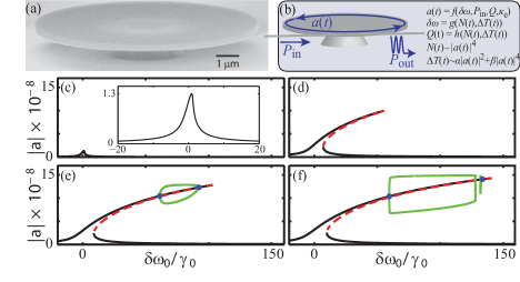
Figure 1: (a) Scanning electron microscope image of a silicon microdisk resonator. (b) Schematic of the physical system, in which a continuous-wave input field results in a periodically oscillating output field. (c)–(f) Steady-state resonance curves for the intracavity field amplitude as a function of normalized detuning. (c) At low power the curve is stable and single valued. (d) As power increases, nonlinear effects grow and the resonance curve bends over, leading to an unstable middle branch (dashed red). (e) Further increase in pump power leads to two simultaneous Hopf bifurcations (blue dots) and the birth of a stable limit cycle (envelope shown in green). (f) When the limit cycle grows sufficiently large, it collides with the middle branch and is destroyed via a homoclinic bifurcation (this collision occurs in four dimensions, and is not visible in this projection.) Pump powers: 0.71 $\mu$W, 45 $\mu$W, 86 $\mu$W, and 120 $\mu$W.

Physical system and model—The physical system we study is a microdisk cavity (Fig. 1(a)) coupled to a single mode optical waveguide. The waveguide is driven with a continuous-wave laser at a specified frequency detuning with respect to a microdisk optical mode. For simplicity, we neglect backscattering effects common in these types of resonators Weiss et al. (1995), and assume that the forward propagating mode of the waveguide excites only the clockwise traveling-wave mode of the microdisk Harayama et al. (1999), which in turn couples back out to the forward propagating mode. Our analysis neglects the Kerr nonlinearity, which has been the focus of considerable experimental Del’Haye et al. (2007); *foster2011; *matsko2013 and theoretical work Lugiato and Lefever (1987); *leo2010; *chembo2010; *matsko2011; *herr2013 in the context of parametric oscillation and frequency comb generation. It also neglects Raman scattering, and instead, focuses on the role of two-photon absorption (TPA). As summarized in Supplemental Material and in Fig. 1(b), a strong enough intracavity field produces two-photon absorption in the silicon material, resulting in heating and thermo-optic dispersion, as well as the generation of free carriers, which cause additional absorption (FCA) and dispersion. The change in the optical loss rate and laser-cavity detuning caused by these effects means that the intracavity field $a(t)$ is coupled to the cavity temperature change $\Delta T(t)$ and the free carrier population $N(t)$.

The physical effects summarized above are described by the following set of coupled differential equations Johnson et al. (2006):

$$\frac{da}{dt}= -\frac{1}{2}\left(\gamma_{0}+\gamma_{e}+\frac{\Gamma_{TPA}\beta_{Si}c^{2}}{V_{TPA}n_{g}^{2}}\left|a(t)\right|^{2}+\frac{\sigma_{Si}cN(t)}{n_{g}}\right)a(t)+i\left(\frac{\omega_{0}\frac{dn_{Si}}{dT}\Delta T(t)}{n_{Si}}+\frac{\omega_{0}\frac{dn_{Si}}{dN}N(t)}{n_{Si}}-\delta\omega_{0}\right)a(t)-i\kappa P_{in}^{1/2}~{},$$ (1a)

$$\frac{dN}{dt}= -\gamma_{fc}N(t)+\frac{\Gamma_{FCA}\beta_{Si}c^{2}}{2\hbar\omega_{0}n_{g}^{2}V_{FCA}^{2}}\left|a(t)\right|^{4}~{},$$ (1b)

$$\frac{d\Delta T}{dt}= -\gamma_{Th}\Delta T(t)+\frac{\Gamma_{disk}}{\rho_{Si}c_{p}V_{disk}}\bigg{(}\gamma_{lin}$$

$$+ \frac{\sigma_{Si}cN(t)}{n_{g}}+\frac{\Gamma_{TPA}\beta_{Si}c^{2}}{V_{TPA}n_{g}^{2}}\left|a(t)\right|^{2}\bigg{)}\left|a(t)\right|^{2}~{},$$ (1c)

(see Supplemental Material Section S2).

Key parameters that we allow to vary include the input laser’s detuning frequency $\delta\omega_{0}=\omega_{0}-\omega_{in}$ (sign is opposite of typical optics convention) and the input power $P_{in}$. We refer the reader to Supplemental Material sections S2 and S3 for details on the system and the values of parameters. For simplicity in analysis, we separate Eq. (1a) into real and imaginary parts, then nondimensionalize to obtain

$$\frac{dU}{d\tau}=- A_{1}U-A_{2}S^{2}U(U^{2}+V^{2})-A_{3}\eta U+A_{4}\eta V$$

$$+ A_{5}xV-A_{6}\theta V~{},$$ (2a)

$$\frac{dV}{d\tau}=- A_{1}V-A_{2}S^{2}V(U^{2}+V^{2})-A_{3}\eta V-A_{4}\eta U$$

$$- A_{5}xU+A_{6}\theta U-A_{7}~{},$$ (2b)

$$\frac{d\eta}{d\tau}=- A_{8}\eta+A_{9}S^{4}(U^{2}+V^{2})^{2}~{},$$ (2c)

$$\frac{d\theta}{d\tau}=- A_{10}\theta+A_{11}S^{2}(U^{2}+V^{2})+A_{12}S^{4}(U^{2}+V^{2})^{2}$$

$$+ A_{13}S^{2}\eta(U^{2}+V^{2})~{},$$ (2d)

where $\tau=\frac{\gamma_{0}}{\sqrt{Q}}t$, $U=\frac{\sqrt{\omega_{0}}}{6Q^{1/4}\sqrt{P_{in}}}\text{Re}(a)$, $V=\frac{\sqrt{\omega_{0}}}{6Q^{1/4}\sqrt{P_{in}}}\text{Im}(a)$, $\eta=\frac{V_{eff}}{Q}N$, and $\theta=\frac{c_{p}}{\gamma_{0}^{2}\sigma_{Si}Q}\Delta T$ are dimensionless real variables of order 1, $A_{1}$ through $A_{13}$ are positive real constants (see Supplemental Material), and $x=\delta\omega_{0}/\gamma_{0}$, $S=(\beta_{Si}\omega_{0}c^{-1}Q^{2}P_{in})^{1/2}$ are the nondimensional corollaries to control parameters $\delta\omega_{0}$ and $P_{in}$.

Regions of Oscillation and Bistability—Figure 1 shows the field amplitude $\left|a\right|$ vs detuning for various driving powers. As power increases, the resonance curve becomes multivalued—bistability and hysteresis becomes possible. At a critical pump power, two simultaneous Hopf bifurcations occur (two pairs of eigenvalues cross the imaginary axis), destabilizing part of the upper branch and leading to the birth of a limit cycle between the two Hopf bifurcations. As pump power is further increased, this limit cycle collides with the unstable fixed point (middle branch), undergoing a homoclinic bifurcation that destroys its stability within a range of detunings—see Fig. 1 panel (f).

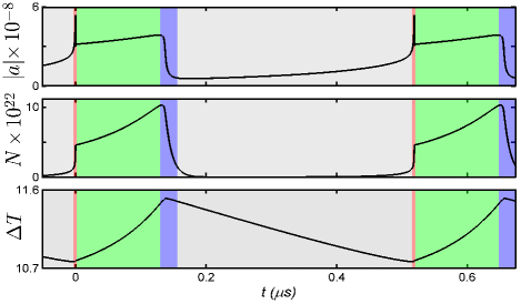
Figure 2: Limit cycle oscillation. Panels show (a) field amplitude $\left|a\right|$, (b) free carrier population $N$ and (c) temperature change $\Delta T$ vs. time. Colors indicate different stages of limit cycle. Pump power is 1 mW ($S=56$) and pump detuning is 0.84 nm above resonance ($\delta\omega_{0}/\gamma_{0}=168$).

Time Domain Behavior—Figure 2 shows the periodic behavior of the system with high pump power and a stable limit cycle. It consists roughly of four stages and can be interpreted physically as follows: the first stage (red) starts at minimum temperature and is driven by rapid TPA. A sharp spike in the field is tempered by linear and nonlinear optical losses and the blue shift of the disk’s resonant frequency due to a denser free carrier population. The free carrier population stabilizes when free carrier recombination ($\gamma_{fc}$) balances with free carrier generation via TPA. Thermal decay ($\gamma_{Th}$) happens more slowly, so cavity temperature doesn’t equilibrate during the spike. The second stage (green) is driven by an increasing temperature red-shifting the disk’s resonant frequency, and consists of steady increases in all variables. A critical temperature is reached (blue), and both the field and free carrier population collapse in conjunction with a sudden drop in TPA. The fourth stage (gray) takes up most of the limit cycle and consists of low activity in the disk while the temperature decreases smoothly.

Figure 3 shows bifurcations that occur in the parameter space of $\delta\omega_{0}/\gamma_{0}$ and $P_{in}$. The limit cycle is “born” in parameter space on the boundary defined by the Hopf-condition (red line) with non-zero period $T$. At powers above a threshold (black asterisk), the limit cycle transitions from supercritical (born with zero amplitude) to sub-critical (born with finite amplitude). In the low power limit, we use a local asymptotic expansion about the Hopf condition to accurately approximate the limit cycle (see Supplemental Material). At higher power we use a multiple-time-scale analysis to ultimately reduce the limit cycle to a one-dimensional relaxation oscillation, and predict the Hopf and homoclinic bifurcations Kuznetsov (1998).

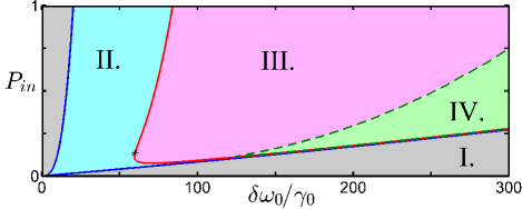
Figure 3: Phase space diagram of system in parameter space of power ($P_{in}$) and detuning ($\delta\omega_{0}/\gamma_{0}$). Region I (gray): monostable (one stable equilibrium), region II (blue): bistable (two stable, one unstable equilibria), region III (pink): stable oscillations (one stable, two unstable equilibria), region IV (green): monostable (one stable, two unstable equilibria). Blue boundary: saddle-node bifurcation, red boundary: Hopf bifurcation, dashed green boundary: homoclinic bifurcation. Black asterisk indicates point where Hopf bifurcation goes from subcritical to supercritical. Power ranges from 0 mW to 1 mW, detuning ranges from 0 nm to 1.5 nm above resonance.

Multiple Time Scales—In their analysis, Johnson et al. suggested that the observed limit cycle can be separated into fast and slow time scales Johnson et al. (2006). Soltani et al. carried out a two-time-scale approximation by assuming changes in temperature are much slower than changes in other variables Soltani et al. (2012); these time scales are apparent in Fig. 2. Here we extend that idea to a convenient approximation in terms of three well-separated time scales. Specifically, the equations governing the field (2a)-(2b), the free carriers (2c), and the temperature (2d) each appear to operate on a different time scale.

Our approach is based upon order of magnitude comparison between the model’s coefficients (see Supplemental Material). The ratio of the coefficients in Eqs. (2a) and (2b) to $A_{1}$ is at least of order one, while the ratio of the coefficients in Eqs. (2c) and (2d) to $A_{1}$ is much less than one Note1 , as long as $A_{3}\gg A_{8}$, which implies that $\sigma_{Si}cQ\gg V_{eff}n_{Si}\gamma_{fc}$ (a less restrictive but necessary relation is $A_{1}\gg A_{8}$, or $\gamma_{0}\gg\gamma_{fc}$). When these relations hold, Eqs. (2a) and (2b), Eq. (2c), and Eq. (2d) evolve on time scales $\tau_{1}=\gamma_{0}t$, $\tau_{2}=\gamma_{fc}t$, and $\tau_{3}=\gamma_{Th}t$ respectively, with $\tau_{1}\gg\tau_{2}$ and $\tau_{1}\gg\tau_{3}$.

Taking the free carrier population $\eta$ and the temperature change $\theta$ to be constant, the solution to equations (2a) and (2b) approach fixed points $U^{\star}=\frac{c_{2}A_{7}}{c_{1}^{2}+c_{2}^{2}}$, $V^{\star}=\frac{c_{1}A_{7}}{c_{1}^{2}+c_{2}^{2}}$ exponentially fast, where $c_{1}=A_{1}+A_{3}\eta$ and $c_{2}=-A_{5}x+A_{6}\theta-A_{4}\eta$. Numerical simulation verifies that the values of $U$ and $V$ are well approximated by these fixed points during the limit cycle. We conclude that the apparent fast dynamics observed in Fig. 2 are slaved to the dynamics of the free carrier population.

Thus, assuming field variables $U$ and $V$ reach equilibrium nearly instantaneously in response to changes in $\eta$ and $\theta$, system (2) reduces to

$$\frac{d\eta}{d\tau}= -A_{8}\eta+{\scriptstyle\frac{A_{9}A_{7}^{4}S^{4}}{\left[(-A_{5}x+A_{6}\theta-A_{4}\eta)^{2}+(A_{1}+A_{3}\eta)^{2}\right]^{2}}}$$ (3a)

$$\frac{d\theta}{d\tau}= -A_{10}\theta+{\scriptstyle\frac{(A_{11}A_{7}^{2}+A_{13}A_{7}^{2}\eta)S^{2}}{(-A_{5}x+A_{6}\theta-A_{4}\eta)^{2}+(A_{1}+A_{3}\eta)^{2}}}$$

$$+ \frac{A_{12}A_{7}^{4}S^{4}}{\left[(-A_{5}x+A_{6}\theta-A_{4}\eta)^{2}+(A_{1}+A_{3}\eta)^{2}\right]^{2}}~{}.$$ (3b)

As expected, this 2D system behaves nearly identically to the 4D system when the above assumptions are satisfied. Figure 4 shows the limit cycle in the phase plane of $\eta$ and $\theta$ along with the nullcline $\frac{d\eta}{d\tau}=0$ (dashed).

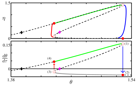
Figure 4: Limit cycle for 2D and 1D reduction in the space of nondimensional free carrier population $\eta$ and temperature change $\theta$ (Eqns. (3) and (4)/(Nonlinear Oscillations and Bifurcations in Silicon Photonic Microresonators) respectively). Top panel: stable periodic solution to 2D model (solid), nullcline $d\eta/d\tau=0$ (dashed), unstable fixed points (filled diamonds), and points of interest in the 1D reduction (filled and open circles). Lower panel: same labeling scheme, solid lines represent branches of nullcline corresponding to 1D limit cycle, arrows indicate instantaneous jumps. Input power is 1 mW ($S=56$) and pump detuning is 0.84 nm above resonance ($x=168$). Color coding indicates portion of cycle with same scheme as Fig. 2.

Note that in Fig. 4 the value of $\eta$ is nearly always either on the nullcline, or changing rapidly with respect to $\theta$. That is, $\frac{d\eta}{d\tau}\gg\frac{d\theta}{d\tau}$ when not on a nullcline. This observation allows us to simplify the system further through a second separation of time scales: we’ll assume that $\eta$ is nearly always at a fixed point. This is valid when $A_{10}\ll A_{8}$ and $A_{10}\ll A_{9}S^{4}$, with the former relation implying that $\gamma_{fc}\gg\gamma_{Th}$. For a disk resting on a pedestal of SiO₂, $\gamma_{Th}\approx 0.2\ \textrm{MHz}$, while $\gamma_{fc}$ is typically $\mathcal{O}(100\ \textrm{MHz})$ Johnson et al. (2006), so the assumption should be valid in our experiments. As long as these conditions and the fast field conditions hold, Eqs. (2a) and (2b), Eq. (2c), and Eq. (2d) evolve on time scales $\tau_{1}=\gamma_{0}t$, $\tau_{2}=\gamma_{fc}t$, and $\tau_{3}=\gamma_{Th}t$ respectively, with $\tau_{1}\gg\tau_{2}\gg\tau_{3}$ ($\gamma_{0}\gg\gamma_{fc}\gg\gamma_{Th}$).

Setting Eq. (3a) equal to zero gives the following parameterization in terms of $\eta$:

$$\theta = \frac{A_{5}x+A_{4}\eta}{A_{6}}\pm\frac{\sqrt{f(\eta)}}{A_{6}\eta}~{},$$ (4)

$$f(\eta) = -A_{3}^{2}\eta^{4}-2A_{1}A_{3}\eta^{3}-A_{1}^{2}\eta^{2}+S^{2}\sqrt{\frac{A_{7}^{4}A_{9}}{A_{8}}}\eta^{3/2}~{},$$

and plugging Eq. (4) into Eq. (3b) gives $\dot{\theta}=\frac{d\theta}{d\tau}$ in terms of $\eta$:

$$\dot{\theta}= -\frac{A_{10}A_{5}x}{A_{6}}+\frac{\sqrt{A_{8}}A_{11}}{\sqrt{A_{9}}}\sqrt{\eta}+\frac{\sqrt{A_{8}}A_{13}}{\sqrt{A_{9}}}\eta^{3/2}$$

$$+\left(\frac{A_{8}A_{12}}{A_{9}}-\frac{A_{10}A_{4}}{A_{6}}\right)\eta\pm\frac{A_{10}\sqrt{f(\eta)}}{A_{6}\eta}$$

Figure 4 illustrates this 1D reduction of the 2D limit cycle. The limit cycle occurs in the region of the graph that is multivalued. The boundaries of the region (maximum and minimum values of $\theta$) mark transition points between the two solution curves.

Estimating the Period of the Limit Cycle—The 1D reduction assumes that the transition between “jump” and “collection” points is instantaneous, separating the limit cycle into four sections: two fast (red and blue sections of Figs. 2 and 4) and two slow (gray and green sections of Figs. 2 and 4). Integrating $\frac{1}{\dot{\theta}(\eta)}\frac{d\theta}{d\eta}$ with respect to $\eta$ along the nullcline from the collection points to the jump points gives the period of the 1D limit cycle. Using approximations to the phase plane branches, we found

$$T \approx 2\frac{\theta^{*}_{1}-\theta^{*}_{3}}{(\dot{\theta}^{*}_{2}-\dot{\theta}^{*}_{3})^{2}}\left[\dot{\theta}^{*}_{3}\ln{\left(\frac{\dot{\theta}^{*}_{3}}{\dot{\theta}^{*}_{2}}\right)}+(\dot{\theta}^{*}_{2}-\dot{\theta}^{*}_{3})\right]$$ (6)

$$+ \frac{\theta^{*}_{1}-\theta^{*}_{3}}{\dot{\theta}^{*}_{1}-\dot{\theta}^{*}_{4}}\ln{\left(\frac{\dot{\theta}^{*}_{1}}{\dot{\theta}^{*}_{4}}\right)}~{},$$

where starred variables indicate known jump and collection points (subscripts refer to numbered critical points in Fig. 4).

Limits of Oscillation—The 1D reduction yields intuitive and simple expressions for the limits of oscillation with respect to detuning. Equations (4) and (Nonlinear Oscillations and Bifurcations in Silicon Photonic Microresonators) imply that changes in detuning simply translate the limit cycle. With increasing detuning, the onset of oscillations occurs when the bottom left “elbow” Fig. 4 (open circle) crosses the $\theta$ axis ($\dot{\theta}^{*}_{3}=0$). The collapse of oscillations through homoclinic bifurcation occurs when the limit cycle collides with the nearby unstable fixed point ($\dot{\theta}^{*}_{4}=0$). The period of the limit cycle diverges near this instability. By using Eqs. (4) and (Nonlinear Oscillations and Bifurcations in Silicon Photonic Microresonators) we can express the bounds of oscillation in terms of all free parameters.

Figure 5 compares the predictions of the 4D model (Eq. (2)), the 2D model (Eq. (3)), and the 1D model (Eqs. (4)/(Nonlinear Oscillations and Bifurcations in Silicon Photonic Microresonators) and (6)) to laboratory data (see Supplemental Material), indicating that they capture the dependence of the period of oscillation on detuning. The 1D reduction overestimates the detuning at which the homoclinic bifurcation occurs due to failure to capture the “overshoot” near instantaneous jumps between branches.

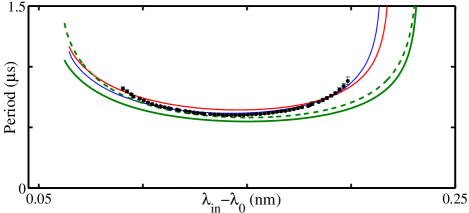
Figure 5: Existence and period of limit cycle. Comparison of 4D (blue), 2D (red), and 1D (green) models from equations (2), (3), (4)/(Nonlinear Oscillations and Bifurcations in Silicon Photonic Microresonators), and (6) to experiment (black points; vertical error bars stem from Lorentzian fits to determine frequency peak locations, and represent one standard deviation in the comb spacing) for $P_{in}=400\ \mu\textrm{W}$, $\lambda_{0}=1609$ nm, $Q=6\times 10^{5}$, $V_{eff}$ = 60 $\left(\frac{\lambda_{0}}{n_{Si}}\right)^{3}$ (fit), $\gamma_{lin}/\gamma_{0}=0.53$ (fit), $\gamma_{Th}=1.4\times 10^{5}$Hz (fit), and $\gamma_{e}/\gamma_{0}=0.08$. Solid line=numerical solution, dashed=analytical approximation.

The dependency of period on other system parameters is generally similar to Fig. 5. Increasing the strength of nonlinear terms usually increases the period of oscillation. In general, changes in period are more severe at the bounds of the limit cycle in parameter space (red and dashed green curves in Fig. 3, see Supplemental Material section S6 for a numerical survey).

Frequency Comb—The self-sustained oscillations of the field inside the cavity produce a frequency comb with spacing on the order of 1 MHz Johnson et al. (2006) (data presented in Supplemental Material). This spacing corresponds to the frequency of the limit cycle, and multiple lines appear since multiple Fourier modes are necessary to represent its non-sinusoidal shape. The amplitude of successive peaks in the comb can be deduced from the structure of the time-domain oscillation. The spike and subsequent abrupt slope-change visible in Fig. 2 is primarily responsible for generating the higher harmonics in the comb and suggest the use of a modified pulse wave for approximate theoretical prediction of the comb envelope. We find that the frequency comb’s higher harmonics decay according to a power law with $n^{-x}$ where $n$ is the index of the harmonic and $x\approx 2$. The power spectrum of a sawtooth pulse wave oscillates about the decay rate of $n^{-2}$ with an oscillatory period (in spikes) of $T/w$, where $T$ is the fundamental period and $w$ is the pulse width. Figure 6 shows the fit of both the data and the 4D numerics to the frequency comb of a sawtooth pulse wave.

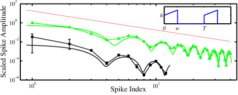
Figure 6: Frequency comb envelope. The frequency comb’s decay for both experimental data (connected black circles) and 4D numerics (connected green triangles) is compared with a best fit saw-tooth pulse wave (solid lines, see inset). Primary spike height is arbitrarily scaled for visual purposes. Red reference line shows $n^{-2}$. Error bars indicate 90$\%$ bootstrap confidence interval derived from Lorentzian fit.

Discussion of Results—We have presented a new approach to modeling the multi-scale oscillatory behavior brought on by nonlinear absorption and dispersion in silicon microdisks. Perturbation theory allows us to reduce dimensionality and gain insight into the underlying dynamics of this nonlinear system, even producing analytic predictions for key properties of the system and key transitions and behavior. The heart of the analysis lies in the separation of time scales between optical, electro-optical, and thermal effects which are characteristic of multiple optoelectronic devices, including the silicon microdisks considered in our work.

Acknowledgements—The authors thanks V. Akysuk, L. Chen, and H. Miao for helpful discussions regarding fabrication of silicon microdisk devices.

See pages - of Microdisk_draft_arXiv2_supplemental.pdf

References

- Orozco et al. (1984) L. A. Orozco, A. T. Rosenberger, and H. J. Kimble, Phys. Rev. Lett. 53, 2547 (1984).
- Segard and Macke (1988) B. Segard and B. Macke, Phys. Rev. Lett. 60, 412 (1988).
- Joshi and Xiao (2003) A. Joshi and M. Xiao, Phys. Rev. Lett. 91, 143904 (2003).
- Armaroli et al. (2011) A. Armaroli, S. Malaguti, G. Bellanca, S. Trillo, A. de Rossi, and S. Combrié, Phys. Rev. A 84, 053816 (2011).
- Gu et al. (2012) T. Gu, N. Petrone, J. F. McMillan, A. van der Zande, M. Yu, G.-Q. Lo, D.-L. Kwong, J. Hone, and C. W. Wong, Nature Photon. 6, 554-559 (2012).
- Kwon et al. (2013) Y.-D. Kwon, M. A. Armen, and H. Mabuchi, arXiv preprint arXiv:1305.1077 (2013).
- Priem et al. (2005) G. Priem, P. Dumon, W. Bogaerts, D. van Thourhout, G. Morthier, and R. Baets, Opt. Express 13, 9623 (2005).
- Johnson et al. (2006) T. J. Johnson, M. Borselli, and O. Painter, Opt. Express 14, 817 (2006).
- Soltani et al. (2012) M. Soltani, S. Yegnanarayanan, Q. Li, A. A. Eftekhar, and A. Adibi, Phys. Rev. A 85, 053819 (2012).
- Xu et al. (2005) Q. Xu, B. Schmidt, S. Pradhan, and M. Lipson, Nature (London) 435, 325 (2005).
- Green et al. (2007) W. M. Green, M. J. Rooks, L. Sekaric, and Y. A. Vlasov, Opt. Express 15, 17106 (2007).
- Reed et al. (2010) G. T. Reed, G. Mashanovich, F. Y. Gardes, and D. J. Thomson, Nature Photon. 4, 518 (2010).
- Xia et al. (2007) F. Xia, L. Sekaric, and Y. Vlasov, Nature Photon. 1, 65 (2007).
- Melloni et al. (2008) A. Melloni, F. Morichetti, C. Ferrari, and M. Martinelli, Opt. Lett. 33, 2389 (2008).
- Cooper et al. (2010) M. L. Cooper, G. Gupta, M. A. Schneider, W. M. J. Green, S. Assefa, F. Xia, Y. A. Vlasov, and S. Mookherjea, Opt. Express 18, 26505 (2010).
- Foster et al. (2006) M. A. Foster, A. C. Turner, J. E. Sharping, B. S. Schmidt, M. Lipson, and A. L. Gaeta, Nature (London) 441, 960 (2006).
- Turner et al. (2008) A. C. Turner, M. A. Foster, A. L. Gaeta, and M. Lipson, Opt. Express 16, 4881 (2008).
- Mabuchi (2009) H. Mabuchi, Phys. Rev. A 80, 045802 (2009).
- Weiss et al. (1995) D. S. Weiss, V. Sandoghdar, J. Hare, V. Lefèvre-Seguin, J.-M. Raimond, and S. Haroche, Opt. Lett. 20, 1835 (1995).
- Harayama et al. (1999) T. Harayama, P. Davis, and K. S. Ikeda, Phys. Rev. Lett. 82, 3803 (1999).
- Del’Haye et al. (2007) P. Del’Haye, A. Schliesser, O. Arcizet, T. Wilken, R. Holzwarth, and T. Kippenberg, Nature 450, 1214 (2007).
- Foster et al. (2011) M. A. Foster, J. S. Levy, O. Kuzucu, K. Saha, M. Lipson, and A. L. Gaeta, Opt. Express 19, 14233 (2011).
- Matsko et al. (2013) A. B. Matsko, W. Liang, A. A. Savchenkov, and L. Maleki, Opt. Lett. 38, 525 (2013).
- Lugiato and Lefever (1987) L. A. Lugiato and R. Lefever, Phys. Rev. Lett. 58, 2209 (1987).
- Leo et al. (2010) F. Leo, S. Coen, P. Kockaert, S.-P. Gorza, P. Emplit, and M. Haelterman, Nature Photon. 4, 471 (2010).
- Chembo and Yu (2010) Y. K. Chembo and N. Yu, Phys. Rev. A 82, 033801 (2010).
- Matsko et al. (2011) A. B. Matsko, A. A. Savchenkov, W. Liang, V. S. Ilchenko, D. Seidel, and L. Maleki, Opt. Lett. 36, 2845 (2011).
- Herr et al. (2013) T. Herr, V. Brasch, J. Jost, C. Wang, N. Kondratiev, M. Gorodetsky, and T. Kippenberg, Nature Photon. 8, 145-152 (2013).
- Kuznetsov (1998) A. Kuznetsov, Elements of applied bifurcation theory, vol. 112 (Springer, 1998).
- (30) The single exception to this separation is the ratio , which is much less than one. This nonlinearity has an insignificant effect on the solution, and excluding it greatly simplifies the analysis (see Supplemental Material).