Supermassive black holes with high accretion rates in active galactic nuclei:
I. First results from a new reverberation mapping campaign

Abstract

We report first results from a large project to measure black hole (BH) mass in high accretion rate active galactic nuclei (AGNs). Such objects may be different from other AGNs in being powered by slim accretion disks and showing saturated accretion luminosities, but both are not yet fully understood. The results are part of a large reverberation mapping (RM) campaign using the 2.4-m Shangri-La telescope at the Yunnan Observatory in China. The goals are to investigate the gas distribution near the BH and the properties of the central accretion disks, to measure BH mass and Eddington ratios, and to test the feasibility of using such objects as a new type of cosmological candles. The paper presents results for three objects, Mrk 335, Mrk 142 and IRAS F12397+3333 with H$\beta$ time lags relative to the 5100Å continuum of $10.6^{+1.7}_{-2.9}$, $6.4^{+0.8}_{-2.2}$ and $11.4^{+2.9}_{-1.9}$ days, respectively. The corresponding BH masses are $(8.3_{-3.2}^{+2.6})\times 10^{6}M_{\odot}$, $(3.4_{-1.2}^{+0.5})\times 10^{6}M_{\odot}$ and $(7.5_{-4.1}^{+4.3})\times 10^{6}M_{\odot}$, and the lower limits on the Eddington ratios 0.6, 2.3, and 4.6 for the minimal radiative efficiency of 0.038. Mrk 142 and IRAS F12397+333 (extinction corrected) clearly deviate from the currently known relation between H$\beta$ lag and continuum luminosity. The three Eddington ratios are beyond the values expected in thin accretion disks and two of them are the largest measured so far among objects with RM-based BH masses. We briefly discuss implications for slim disks, BH growth and cosmology.

1 Introduction

Active galactic nuclei (AGNs) are powered by accretion onto supermassive black holes (SMBHs) located at the centers of their host galaxies. Most of the information about the physical conditions in the vicinity of the BH is obtained through spectroscopy of such sources. In addition, the temporal behaviors of the continuum and emission lines in such objects provide useful information about the distribution and emissivity of the line emitting gas and, through reverberation mapping (RM), a way to measure the mass of the central BH (Bahcall et al. 1972; Blandford & McKee 1982; Netzer 1990; Peterson 1993; Netzer & Peterson 1997; Peterson 2013 and references therein). RM experiments, based on the response of the broad emission lines to the continuum variations, have provided reliable estimates of the lag between the continuum and the broad emission line light curves in about 50 AGNs (e.g., Kaspi et al. 2000; Peterson et al 2004; Kaspi et al. 2005; Bentz et al. 2009a,b; Denney et al. 2010; Bentz et al. 2013). This information, combined with a measure of the gas velocity in the broad line region (BLR) was used to obtain an estimate of the BH mass. This involves expressions of the type,

$$M_{\bullet}=f_{{}_{\rm BLR}}\frac{R_{{}_{\rm BLR}}v^{2}}{G},$$ (1)

where $M_{\bullet}$ is the BH mass, $f_{{}_{\rm BLR}}$ is a factor that includes information about the geometry and kinematics of the BLR gas, $R_{{}_{\rm BLR}}$ is the responsivity weighted radius of the BLR for the emission line in question, and $v$ is a measure of the velocity in the line emitting gas, e.g., the full width at half maximum (FWHM) ($V_{{}_{\rm FWHM}}$) or the “line dispersion” ($\sigma_{\rm line}$, see Peterson et al. 2004 and references therein). For a virialized BLR with close to a spherical geometry, $f_{{}_{\rm BLR}}\sim 1$ for velocity characterized by $V_{{}_{\rm FWHM}}$ (e.g., Netzer and Marziani 2010) and $f_{{}_{\rm BLR}}\sim 5.5$ for velocity characterized by $\sigma_{\rm line}$ (Park et al 2012; Woo et al. 2013 and references therein). The only practical way to calibrate the value of $f_{{}_{\rm BLR}}$ is in AGNs with measured stellar velocity dispersion in the bulge of the galaxy, $\sigma_{*}$, through comparison with BH mass estimates based on the well-established $M_{\bullet}-\sigma_{*}$ relationship in non-active galaxies (Ferrarese et al. 2001; Onken et al. 2004; Park et al. 2012; Woo et al. 2013). The data presented in Woo et al. (2013), suggests that $f_{{}_{\rm BLR}}$ does not depend on the Eddington ratio. This includes the 7 narrow line Seyfert 1 galaxies (NLS1s) in that sample: Mrk 110, Mrk 202, Mrk 590, Mrk 766, NGC 4051, NGC 4748 and NGC 7469.

All RM campaigns show tight $R_{{}_{\rm BLR}}-L$ relations, where $L$ is a measure of $\lambda L_{\lambda}$ in the optical-UV part of the spectral energy distribution (SED), for both H$\beta$ and the C iv$\lambda 1549$ emission lines (Kaspi et al. 2007; Denney et al. 2013; Bentz et al. 2013). Such relationships provide an indirect way to estimate the BLR size, and hence $M_{\bullet}$, from “single epoch” spectra assuming virialized BLRs. Such methods are routinely used in studies of BH mass and accretion rate distributions in large AGN samples such as the Sloan Digital Sky Survey (SDSS, see e.g., McLure & Dunlop 2004; Wang et al. 2006, 2009; Netzer et al. 2007; Netzer & Trakhtenbrot 2007; Hu et al. 2008; Vestergaard & Osmer 2009; Shen 2009; Trakhtenbrot & Netzer 2012; Kelly & Shen 2013). The more reliable measurements of $M_{\bullet}$ based on RM experiments, are available for only about 50 AGNs with directly measured $R_{{}_{\rm BLR}}$. Most of these sources are “slow accretors”, i.e., their luminosities are well below the Eddington limit.

In this paper we assume that all BHs are powered by accretion via a central, optically thick accretion flow that takes the shape of an accretion disk (AD). We use the same general notation for all such flows, where

$$\dot{m}=\frac{L_{\rm Bol}}{L_{\rm Edd}}=\frac{\eta\dot{M}c^{2}}{L_{\rm Edd}}=\eta\dot{\mathscr{M}},$$ (2)

is the “Eddington ratio”. Here, $L_{\rm Bol}$ and $L_{\rm Edd}$ are the bolometric and Eddington luminosity, respectively, $\dot{M}$ is the mass accretion rate through the disk, $\eta$ is the efficiency of converting accreted mass to radiation and $\dot{\mathscr{M}}=\dot{M}c^{2}/L_{\rm Edd}$ is the “Eddington rate”. The Eddington luminosity we use assumes solar composition gas and is given by $L_{\rm Edd}=1.5\times 10^{45}\left(M_{\bullet}/10^{7}M_{\odot}\right)\rm erg~{}s^{-1}$.

In principle, the Eddington ratio $(\dot{m}$) is a measurable property obtained from the measured $M_{\bullet}$ and the known SED. The Eddington rate is a more theoretical concept that is related to the physics and geometry of the accretion flow. The radiation of geometrically thin ADs, like those based on the black body disk model of Shakura and Sunyaev (1973; hereafter SS disk) depend only on the location of the last stable orbit (Bardeen et al. 1972). Thus, $\eta_{{}_{\rm SS}}\approx(0.057,0.32,0.038)$ for spin parameters of $a=(0,0.998,-1)$, respectively. However, thicker “slim disks” are subject to radial advection which can significantly reduce the efficiency. Here, $\eta_{{}_{\rm Slim}}\propto\dot{\mathscr{M}}^{-1}$ and is only weakly dependent on the BH spin. The canonic models of slim disks (e.g., Wang & Zhou 1999a; Wang & Netzer 2003) suggest a logarithmic relation between $\dot{m}$ and $\dot{\mathscr{M}}$ in such systems. For example, in such cases $\dot{m}\approx(2-3)$ for $1\lesssim\dot{\mathscr{M}}\lesssim 200$ (Abramowicz et al. 1988; Wang et al. 1999b Mineshige et al. 2000). In principle, $\dot{m}$ can be determined by observations but the determination of $\dot{\mathscr{M}}$ is more problematic since it depends on the specific slim disk model. This has important implications to the process of cosmic growth of BHs, the duty cycle of activity, etc.

A recent paper by Wang et al. (2013) suggests that super-Eddington accreting massive black holes (SEAMBHs), those objects with $\dot{\mathscr{M}}\gg 1$ and 2-10 keV photon index ($\Gamma_{2-10}$) larger than 2, can be used as a new type of cosmological candles. The method is based on the fact that the bolometric luminosity of slim accretion disks around massive BHs tends to saturate at super-Eddington rates. Under such conditions, $L_{\rm Bol}\propto M_{\bullet}$ with only a weak logarithmic dependence on $\dot{\mathscr{M}}$. This idea, if confirmed by more accurate measurements, can provide a useful tool for measuring cosmological distances at high redshifts, where supernovae (SNe) are hard to detect or are rare (Hook 2012) because of their slow evolution (Kobayashi & Nomota 2009). SEAMBHs are very luminous, and can be easily detected in large numbers up to very high redshifts (Netzer and Trakhtenbrot 2013). In addition, their properties may not depend in any way on galaxy evolution. However, there are a very small number of such sources with accurately measured BH mass in the local universe and a systematic study is necessary to test these ideas.

We have started a large observational project, in China, aimed at increasing considerably the number of high$-\dot{m}$ systems with good RM measurements that will allow reliable estimates of $M_{\bullet}$. The main scientific goals are: 1) Understand the physical properties of slim accretion disks. 2) Probe the physics and dynamics of the BLR gas in very fast accretors. 3) Improve the understanding of co-evolution of galaxies and their central BHs in extreme cases where mass accretion, and hence BH growth, are very fast. 4) Use the improved mass and accretion rate measurements to calibrate SEAMBHs as cosmological candles.

In this paper, the first in a series, we outline the overall program, explain the observational aspects and introduce our first results for three BHs that are very fast accretors. In §2 we describe the target selection, the observational setup and the data reduction procedure. In §3 we present the first results of the project and draw preliminary conclusions. Throughout this work we assume a $\Lambda$CDM cosmology with $H_{0}=67\,{\mathrm{km~{}s^{-1}Mpc^{-1}}}$, $\Omega_{m}=0.32$ and $\Omega_{\Lambda}=0.68$ in light of Planck observations (Ade et al. 2013).

2 Observations and reduction

2.1 Target selections

The most important criterion for the selection of targets is based on their normalized accretion rate as estimated by the (less accurate) single-epoch method. In particular, we search for objects with $\dot{m}\geq 1$. As explained, the suggestion is that in such cases, the radiative efficiency $\eta$ is no longer a simple function of the BH spin and advection becomes an important process that affects the source luminosity. We decided to avoid radio loud AGNs although, in a few cases, a radio loud source was discovered after the project had begun. Such cases will be discussed separately.

Selecting AGNs by their high accretion rates depends on their $L_{\rm Bol}$ which in itself depends on the SED. Unfortunately, in standard ADs, much of the radiation is emitted beyond the Lyman limit at 912Å  (Laor and Netzer 1989; Elvis et al. 1994; Marconi et al. 2004; Richards et al. 2006; Davis and Laor 2011; Elvis et al. 2012). According to the standard SS model, the optical bolometric correction factor, $\kappa_{\rm B}$, i.e., the factor converting $\lambda L_{\lambda}$ measured at optical wavelengths to $L_{\rm Bol}$, depends on the accretion rate and BH mass such that $\kappa_{\rm B}\propto(\dot{m}/M_{\bullet})^{1/3}$. For ADs around $10^{8}-10^{9}M_{\odot}$ black holes, this agrees with global empirical estimates that suggest $\kappa_{\rm B}\sim 5-10$ (e.g., Marconi et al. 2004). However, much larger and much smaller values of $\kappa_{\rm B}$ are predicted by thin AD models for smaller and larger BHs, respectively (see specific examples in Netzer and Trakhtenbrot 2013). Since most of the $\sim 50$ measured BH masses in the RM campaign have BH masses that fall below $10^{8}$$M_{\odot}$, we suspect that $\dot{m}$ in at least several of these sources has been underestimated in the past. Thus, at least some of these sources can be SEAMBHs.

Alternatively, we can select targets based on the slope of their 2-10 keV X-ray continuum. As argued in Wang et al. (2013), some SEAMBH models predict that such objects would show steeper X-ray slopes compared with low-$\dot{m}$ sources. While a possible $\dot{m}-\Gamma_{2-10}$ relation has been suggested by Wang et al. (2013), this depends on the poorly understood disk-corona structure. The underlying physics is based on the link between the accretion rate in the cold gas phase, the increased emission from the UV and optical bands, and the enhancement of Comptonization cooling, leading to a suppressed hot corona emission. A correlation between $\dot{m}$ and $\Gamma_{2-10}$ has indeed been reported in both low and high luminosity AGNs (see e.g., Wang et al. 2004; Risaliti et al. 2009; Zhou & Zhang 2010; Shemmer et al. 2006; Brightman et al. 2013). A sample of 60 SEAMBH candidates selected from the literature was presented by Wang et al. (2013). The $\dot{m}-\Gamma_{2-10}$ correlation in this sample is strong but with a large scatter. Much of the scatter can be the result of the uncertain BH masses and bolometric luminosities of these sources.

Our target selection follows several criteria that remove the dependence of the disk structure on the uncertain $L_{\rm Bol}$:

1. The sources are NLS1s suspected to be SEAMBHs. Their $L_{\rm Bol}$ and $M_{\bullet}$ are based on the single epoch mass determination method and satisfy $\dot{m}>1$. Their Eddington rates are based on the SS thin disk model and hence:

   $$\dot{m}_{{}_{\rm SS}}\simeq 20.1\left(\frac{L_{44}}{\cos i}\right)^{3/2}M_{7}^{-2}\eta_{{}_{\rm SS}}\,,$$ (3)

   where $L_{44}=\lambda L_{\lambda}/10^{44}\rm erg~{}s^{-1}$ at $\lambda=5100$Å, $M_{7}=M_{\bullet}/10^{7}M_{\odot}$ and $i$ is the inclination angle. We require that $\dot{m}_{{}_{\rm SS}}>1$ for $\cos i=0.75$ (an inclination typical of type-I AGNs that cannot be observed from a much larger inclination angle due to obscuration by the central torus). This expression contains the unknown value of $\eta$ due to the unknown BH spin ($a$). However, a lower limit on $\dot{m}_{{}_{\rm SS}}$ can be obtained by assuming the lowest possible efficiency of thin ADs, $\eta_{{}_{\rm SS}}=0.038$, corresponding to a spin parameter of $a=-1$. We should point out, again, that $\dot{m}_{{}_{\rm SS}}$ given by Eqn. 3 is a lower limit for the Eddington ratios $\dot{m}$ if BH accretion proceeds via a slim AD.

2. The targeted S/N is high enough to enable 2D velocity-resolved RM in the H$\beta$ and Mg ii $\lambda 2798$ lines.

3. The 2-10 keV photon index is very steep, $\Gamma_{2-10}>2$.

4. Targets can be followed from the ground for a period of at least 80 to 180 days for low and high redshift AGNs, respectively.

5. Objects with proven continuum variations. We note that there is some evidence that the variability amplitudes of AGNs are anti-correlated with Eddington ratios (e.g., Ai et al. 2013; Zuo et al. 2012). In particular, some NLS1s show small optical continuum variations (Giannuzzo et al 1996, 1998), but some are very small (Shemmer & Netzer 2000; Klimek et al. 2004; Yip et al. 2009). However, significant variations are found in many SDSS NLS1s located in the Strip 82 region (Ai et al. 2013). We chose sources from the Catalina database and excluded candidates showing variations of less than 10% in the Catalina light curves.

2.2 Photometric and spectrophotometric observations

2.2.1 The Shangri-La telescope and spectrograph

All the spectroscopy and imaging observations reported here were obtained with the Shangri-La telescope (SLT: IAU site code O44) at the Lijiang Station of the Yunnan Observatory of the Chinese Academy of Sciences. The SLT started its operation in 2008. This is a 2.4 m alt-azimuth mounted Ritchey-Chr$\mathrm{\acute{e}}$tien telescope with a field de-rotator enabling to position two objects along the same long slit. The RMS pointing error is about 2 arcsec rms, and the tracking accuracy with autoguiding is better than $0.5^{\prime\prime}/$hour. The longitude of the station is $100^{\circ}~{}01^{\prime}~{}51^{\prime\prime}$ E, the latitude $26^{\circ}~{}42^{\prime}~{}32^{\prime\prime}$ N, and the altitude 3193 m. The site has two observing seasons: a rainy season that lasts from June to mid-September, with very little clear time, and a dry season, from mid-September until May, when most nights are clear. The annually averaged seeing is $\sim 1^{\prime\prime}.5$ in terms of the FWHM of stars (measured with YFOSC), ranging from $0^{\prime\prime}.7$ to $2^{\prime\prime}.0$.

The YFOSC (Yunnan Faint Object Spectrograph and Camera), built in 2010 by the astronomical instrumentation team at the Niels Bohr Institute, is similar to the EFOSC (ESO Faint Object Spectrograph and Camera), but with an additional focal reducer. It started its operation in 2011. YFOSC is a versatile instrument for low resolution spectroscopy and imaging, working at the Cassegrain focus. The CCD chip is an e2v CCD42-90 Back Illuminated Deep Depletion $2048\times 4608$ pixel Scientific CCD Sensor whose pixel size is 13.5 mm, pixel scale $0.283^{\prime\prime}$ pixel^-1, covering a $10^{\prime}\times 10^{\prime}$ field of view. Switching from photometry to spectroscopy is done automatically and takes less than one second. The spectrograph is equipped with a large number of grisms with different dispersions and can be used in a long slit mode as well as with several fixed apertures.

2.2.2 Spectrophotometry

Our RM campaign started in October 2012. We focused on objects whose $L_{5100}$ indicates H$\beta$ lag of up to 30 days as judged by the expression given in Bentz et al. (2009a). The typical sampling frequency is very high and for most sources we managed to obtain high quality spectra almost every night. Observations of a particular object were terminated when a clear line-to-continuum lag was detected and measured. The mean number of nights per source was about $90$ and the mean monitoring period about 8 times the H$\beta$ delay.

We took advantage of the long slit capability of the YFOSC and observed a nearby standard star along the slit for all objects. As explained in detail in the original papers adopting this method (Maoz et al. 1990; Kaspi et al. 2000), this ensures high accuracy relative flux measurements even during times of relatively poor observing conditions. Selection of comparison stars is based on the images of the SDSS and the typical separation between targets and comparison stars is $\sim 1^{\prime}-3^{\prime}$. Given the seeing conditions, the entrance slit was fixed at projected width of $2^{\prime\prime}.5$.

All the spectra were obtained using YFOSC with Grism 14 which provides a resolution of 92 Å mm^-1 (1.8Å pixel^-1) and covers the wavelength range of $3800-7200$Å. For each object/comparison star, we obtained three consecutive exposures in order to remove cosmic-rays and estimate the systematic flux calibration errors. Standard neon and helium lamps are used for wavelength calibration. The spectroscopic data are reduced using standard IRAF v2.16 routines before absolute flux calibration. All spectra are extracted in a uniform, rather large extraction aperture of 30 pixels ($\sim$ 8.5 arcsec) to avoid light losses.

The flux calibration is done in two steps: (1) Absolute flux spectra of the comparison stars are generated using the observations of spectrophotometric standards in several nights of good weather conditions. This results in fiducial fluxed spectra for all comparison stars. (2) For each object/comparison star pair, a sensitivity function is obtained by comparing the spectrum of the star to the fiducial spectrum. This produces a sensitivity function that is applied to calibrate the observed AGN spectrum. This step resembles the IRAF sensfunc and calibration, and it also resembles the method of AGN/star ratio that was used by Maoz et al. (1990) and Kaspi et al. (2000).

2.2.3 Photometric observations

We also made photometric observations through a Johnson $V$-filter of all targets and comparison stars. This allows us to test the quality of the comparison star calibration and the continuum light curves. The observations are done just before the spectroscopic observations with typical exposure times of 4–5 minutes for a $m_{V}=15-16$ target.

The images are reduced using standard IRAF procedures. We perform differential photometry of the targets relative to several other stars in the same field. The number of comparison stars is typically $3-4$. The radius of the aperture photometry is $10^{\prime\prime}$ and the typical photometric accuracy 1–2%.

2.3 Line and continuum light curves

2.3.1 light curve measurements

We use two continuum bands, 4760-4790Å  and 5085-5115Å, in the rest frame, to set the continuum underneath the H$\beta$ emission line. We then integrate the continuum-subtracted H$\beta$ flux between 4810 and 4910Å. The red limit of the band is chosen to exclude the Fe ii  line at around 4924Å, which is strong in some of the objects. Two kinds of error bars are calculated for the continuum flux. First, for the consecutive exposures in the same night, after flux calibration by the comparison star described above, the mean flux of each exposure over the entire wavelength range is calculated. Then the mean fluxes of exposures are divided by that of the combined spectrum in that night to yield flux ratios. The largest deviation of the ratios from unity is used as an error bar. Second, the Poisson error of the measured continuum flux is calculated from the combined spectrum in the corresponding continuum band. Typically the two error bars are comparable (both $\sim 1\%$), but there are exceptions where one of the two dominates. The two error bars are summed in quadrature as the final uncertainty of the continuum flux. For the error bar of the emission line flux, only Poisson noise is calculated. The first kind of error, difference between consecutive exposures, includes the change in the host galaxy contamination. The emission line fluxes should be unaffected by such changes. Thus, the difference between consecutive exposures is not inherited.

The above error bars on the continuum flux do not account for systematic uncertainties that can be caused by poor weather conditions, bright moon, telescope tracking inaccuracies, slit positioning, etc. These are manifested as flux differences between adjacent nights that are significantly larger than the mean continuum variations over this period (the variability time scale for all sources is much longer than one day). To estimate these uncertainties we first smooth the continuum light curve with a median filter of 5–6 points. We then subtract this median-smoothed light curve from the original light curve and obtained the standard deviation from the residuals. This serves as an estimate of the systematic uncertainty. The systematic uncertainties are usually larger than those associated with the measurements in one night and are therefore the largest contributors to the total errors that go into the CCF analysis and the calculated time-lag uncertainties (there are several exceptions where errors on individual points are larger than the systematic uncertainties). This method is very similar to the one described by Peterson et al. (1998) and Bentz et al. (2009).

We constructed line and continuum light curves for all of the sources. Some of the photometric observations are seriously influenced by moon light when a target is close to the moon. While the spectroscopic light curves follow the photometric ones, the agreement between the two is influenced by host galaxy contamination. This is the result of the constant slit width in all observations that may result in different host galaxy contributions on different nights. The leading factors are seeing variations, inaccurate centering of the target and inaccurate tracking. The host galaxy contribution can change slightly from one night to the next, which can affect the AGN light curve.

2.3.2 Variability characteristics

To characterize the continuum variability of the sources we use the variability characteristic $F_{var}$ defined by Rodríguez-Pascual et al. (1997),

$$F_{\rm var}=\frac{\left(\sigma^{2}-\Delta^{2}\right)^{1/2}}{\langle F\rangle}\,,$$ (4)

where $\langle F\rangle=N^{-1}\sum_{i}^{N}F_{i}$ is the averaged flux, $N$ is the number of observations and

$$\sigma^{2}=\frac{1}{N-1}\sum_{i}^{N}\left(F_{i}-\langle F\rangle\right)^{2};~{}~{}~{}~{}\Delta^{2}=\frac{1}{N}\sum_{i}^{N}\Delta_{i}^{2}.$$ (5)

Here $\Delta_{i}$ represents the uncertainty on the flux $F_{i}$. Below we apply Eqn (4) to the $V$-band, $F_{\rm H\beta}$ and $F_{5100}$ light curves.

2.3.3 Cross correlation analysis

We employed two standard methods to analyze the correlation between the line and continuum light curves: the interpolated cross-correlation function (ICCF, Gaskell & Sparke 1986; Gaskell & Peterson 1987) and the Z-transformed discrete correlation function (ZDCF, Alexander 1997). The latter is an improvement on the discrete correlation function (DCF) of Edelson & Krolik (1988). The results of the two are in excellent agreement and we only quote the time lags obtained with the ICCF.

The delay of the emission lines relative to the continuum variations is determined either by measuring the location of the peak of the cross-correlation function (CCF) ($r_{\mathrm{max}}$) or the centroid of the points around the peak above a certain threshold, e.g., 80% ($r\geq 0.8r_{\mathrm{max}}$). We note the two by $\tau_{\mathrm{peak}}$ and $\tau_{\mathrm{cent}}$. The uncertainties on $\tau_{\mathrm{peak}}$ and $\tau_{\mathrm{cent}}$ were calculated with the “flux randomization(FR)/random subset sampling (RSS)” method. This procedure is described in Peterson et al. (1998; 2004) and will not be repeated here.

2.4 Host galaxy contamination

In order to obtain the Eddington ratios (Eqn. 3), we have to subtract the contaminations of host galaxies. Following the scheme described in Bentz et al. (2009a), we estimated the host galaxy contribution to the observed AGN flux at 5100Å  using archival Hubble Space Telescope (HST) images that are available for all our targets. In a case of more than one HST observation, we chose those images with the longest exposure times in the optical band.

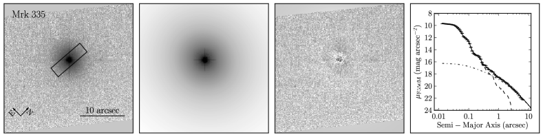
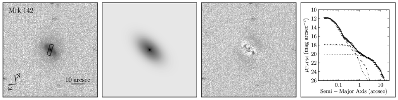
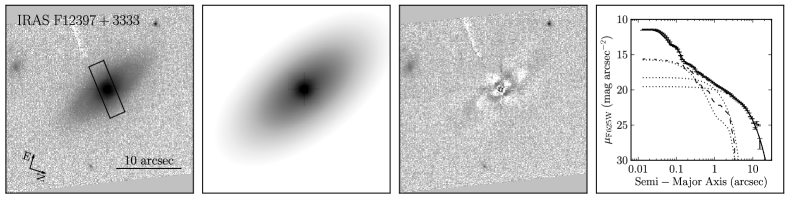
Figure 1: Hubble Space Telescope images of Mrk 335, Mrk 142 and IRAS F12397+3333. The left panels show the original images and the small boxes illustrate the spectroscopic aperture used to extract the spectrum. The 2nd column shows model images, the 3rd one the residuals obtained after subtracting the fitted model. The 4th column shows one-dimensional surface profiles of the three galaxies. Points with error bars are observed data, solid lines are the best-fit models, dashed lines are PSFs, dash-dotted lines are host profiles and dotted lines are the components (Sérsic profiles) used to model the host galaxy light.

The procedure used here is quite standard and its main features are summarized here for clarity. We retrieve from the archive the calibrated data that were reduced by the latest version of the pipeline, and the best reference files. All of the exposures for a single object are combined with AstroDrizzle v1.0.2 task in the DrizzlePac package to clean cosmic rays and make one distortion-corrected image of the host galaxy. Only the pixels flagged as good in the data quality frames are included in the combined images. Some exposures include saturated pixels. These were removed prior to the final combination of all data. Thus, all pixels marked with zeros in weighting Astrodrizzle output, (i.e., no good pixel from any exposure) are masked out in the following fitting processes. Examples of the final combined distortion-free images are shown in the left panels of Figure 1 with spectroscopic monitoring apertures overlaid. The diagram confirms that galaxy contribution to the observed fluxes at 5100Å is non-negligible in all three cases.

We use GALFIT v3.0 (Peng et al. 2002; 2010) to model the surface brightness distribution of the three host galaxies. The GALFIT algorithm fits two dimensional analytic functions to galaxies and point sources. Each of the objects in this study is fitted with a point-spread function (PSF) to model the AGN, one to several Sérsic profiles to model the host galaxy, and a constant to model the sky background. PSFs were generated for each AGN by creating a distorted PSF model at its detector position in each of the exposed frames using TinyTim package (Krist 1993) and combining these models by Astrodrizzle using the same configuration that was used to combine the AGN images. Sérsic profiles are employed to model the various host galaxy components such as bulges, disks and bars. Thus the surface brightness is expressed as

$$\Sigma(R)=\Sigma_{e}\exp\left\{-\kappa_{0}\left[\left(\frac{R}{R_{e}}\right)^{1/n}-1\right]\right\}\,,$$ (6)

where $\Sigma_{e}$ is the surface brightness at the effective radius $R_{e}$, $n$ is the Sérsic power-law index and $\kappa_{0}$ is coupled to $n$ to make sure that half of the flux is within $R_{e}$ (see details in Peng et al. 2002; 2010) ($n=1$ represents a galactic disk and $n=4$ a bulge). We set no constraint on $n$ when fitting bulge, bar or elliptical host, but fix $n=1$ to model the disk component.

At least one Sérsic component was required to model the galaxy in addition to the PSF and sky components, and more were added if needed. For some cases where the PSF modeled by TinyTim does not match the nuclear surface brightness distribution well (see Krist 2003; Kim et al. 2008), an additional Sérsic component with small effective radius was used to modify the mismatch. When the field of view (FOV) of the HST instrument [e.g., High Resolution Channel (HRC) of the Advanced Camera for Surveys (ACS)] is small, the area in the edge of the image used to constrain the fitted sky value was limited. We carefully adjusted the initial parameters to make sure the residuals and $\chi^{2}$ were minimized. Other bright objects in the FOV of our targets were masked out.

Having completed the host galaxy modeling, we subtracted the PSF and sky components from the images of each object and extracted from the PSF-sky-free images the total counts due to the host galaxy inside the slit of the spectrograph. These counts were transformed to flux density units. Because of the difference between the pivot wavelength of the HST filter and the rest-frame 5100Å, we used a bulge template spectrum (Kinney et al. 1996) to determine the required color correction. The template is redshifted and reddened by Galactic extinction based on the dust extinction map of Schlafly & Finkbeiner (2011). The synphot package is then employed to convolve the HST passband with the template to simulate the photometry.

Normalizing the counts to the observed total counts in the aperture provides the host galaxy flux at 5100Å. We adopted a nominal 10% uncertainty on the host galaxy contributions due to the modeling procedures (see also analysis in Bentz et al. 2013).

3 Results and discussion

3.1 General results

In this first paper of the series we report the observations of three objects: Mrk 142, Mrk 335 and IRAS F12397+3333. Information on the three targets and comparison stars is given in Table 1 as well as the variability parameters ($F_{\rm var}$) for the continuum and the H$\beta$ emission line. Table 2 gives the data for the continuum and H$\beta$ light curves. Mrk 142 was previously mapped by the LAMP collaboration (Bentz et al. 2009b). Mrk 335 has been monitored in 2 earlier campaigns (Kassebaum et al. 1997; Grier et al. 2012) and IRAS F12397+3333 is reported here for the first time. Table 3 and Fig. 1 present data and images related to the host galaxy treatment in the three sources (see captions for details). The HST images of Mrk 142 and Mrk 335 have been analyzed by Bentz et al. (2009a; 2013) and the one for IRAS F12397+3333 has been treated by Mathur et al. (2012) who followed the same scheme described in Bentz et al. (2009a). Our results are consistent with both these earlier studies.

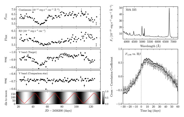
Figure 2: Results for Mrk 335. From top to bottom and from left to right: 1. $F_{5100}$ light curve. 2. H$\beta$ light curve. 3. $V-$band light curve 4. $V-$band light curve of the comparison star. 5. Moon phases and angular separation, in degrees, between the target and the moon (red line). The Moon brightness is coded on the right side of the panel (1.0 is full moon). 6. Mean observed spectrum. 7. The CCF of $F_{5100}$$-$H$\beta$ light curves. Points with error bars are from the ZDCF method and solid line from the ICCF method. Note the effect of the moon on the comparison star magnitude. The bars plotted in the right lower corners of $F_{5100}$ and $F_{\rm H\beta}$ light curves are the systematic uncertainties (see details in §2.3.1).

Figures $2-4$ show mean observed spectra, light curves and CCFs for the three sources. As described below, we found that moon phases and the angular separation between the Moon and the target are the main factors affecting the $V-$band light curve. We demonstrate this in Fig. 2 for one of the sources (Mrk 335) and do not use these light curves any more since they are inferior to the $F_{5100}$ light curves in all three sources. The variability characteristics, $F_{\rm var}$, calculated from the light curves are given in Table 1. The averaged variability is typically $\sim 5\%$ over the monitoring campaign. The largest peaks or dips are significantly larger than this value. For Mrk 335, Mrk 142 and IRAS F12397+3333, they show $F_{5100}$ and H$\beta$ variations of $(F_{5100},{\rm H}\beta)\approx$ $(15\%,10\%)$, $(25\%,20\%)$, $(15\%,10\%)$, respectively. All values are significantly larger than the uncertainties associated with our line and continuum measurements.

The lags computed from the CCFs of the H$\beta$ emission line versus the $F_{5100}$ light curves are tabulated in Table 4 and discussed in §3.2. We prefer the use of $F_{5100}$ over the $V$-band since the latter may be influenced by the strong emission lines of H$\beta$ and Fe ii  that can slightly affect the lag determination. The monochromatic luminosities, $L_{5100}$, calculated after allowing for Galactic extinction based on Schlafly & Finkbeiner (2011), are listed in Table 5. We used the centroid time lag ($\tau_{\rm cent}$) to indicate our best value of $R_{{}_{\rm BLR}}$ that enters the calculation of the BH mass.

Our BH mass measurements are based on the FWHM of the broad H$\beta$ lines as measured from the mean spectra. The subtraction of the narrow H$\beta$ component is rather uncertain because of the very smooth line profiles and the limited spectral resolution of our observations (about 500 km/sec based on a comparison with the SDSS spectra). Similar to the approach used in Hu et al. (2012), we fitted the entire H$\beta$ profile with a narrow Gaussian component ($F_{\rm N}$) and a broad Gaussian-Hermite component ($F_{\rm B}$). For a typical AGN with luminosity similar to the ones measured in our sample, $F_{\rm N}/F_{\rm[O~{}III]}\simeq 0.1$, where $F_{\rm[O~{}III]}$ is the flux of the narrow [O iii]$\lambda 5007$ line. We used this ratio, and the shift and FWHM of the [O iii]$\lambda 5007$ line, to define $F_{\rm N}$. This was subtracted from the total profile to obtain the measured FWHM(broad H$\beta$). The uncertainty is obtained by following the same procedure assuming a) $F_{\rm N}=0$ and b) $F_{\rm N}=0.2F_{\rm[O~{}III]}$. Finally we obtained the intrinsic FWHM(broad H$\beta$) by allowing for the instrumental broadening. The FWHMs and their uncertainties are listed in Table 5.

Regarding the preferred velocity measure, there are two options: $V_{{}_{\rm FWHM}}$ and $\sigma_{\rm line}$ (see §1 for definitions and references). The mean values for both are obtained through a comparison with the $M_{\bullet}-\sigma_{*}$ relationship in non-active galaxies. The most recent results based on 25 AGNs with reliably measured $\sigma_{*}$ are those of Woo et al (2013) who obtained $f_{{}_{\rm BLR}}(\sigma_{\rm line})=5.1-5.9$, depending on the exact method used. The uncertainty on these numbers are about $\pm 1.5$. Netzer and Marziani (2010) used the $V_{{}_{\rm FWHM}}$-based method and the somewhat inferior samples of Onken et al. (2004) and of Woo et al. (2010) to obtain $f_{{}_{\rm BLR}}(V_{{}_{\rm FWHM}})=1.0$. This is confirmed by the more recent results of Woo (2013, private communication) that provides $f_{{}_{\rm BLR}}(V_{{}_{\rm FWHM}})$ for the above sample of 25 AGNs. The results of this work is $f_{{}_{\rm BLR}}(V_{{}_{\rm FWHM}})=0.98^{+0.28}_{-0.22}$, i.e. similar to the scatter of $f_{{}_{\rm BLR}}(\sigma_{\rm line}$). Since for a Gaussian line profile $V_{{}_{\rm FWHM}}\simeq 2.35\times\sigma_{\rm line}$, the two methods are basically identical given the uncertainties.

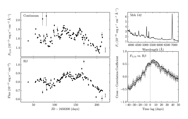
Figure 3: Results for Mrk 142. The left two panels are light curves of continuum at 5100Å  and H$\beta$, and the right two panels are mean spectrum and CCF.

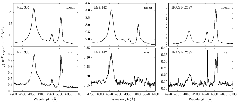
Figure 5: Mean and RMS spectra (observed flux vs. rest-frame wavelength) of the three objects. The spectra are normalized to roughly the same vertical scale to enable a clearer comparison. Note the much noiser RMS spectrum and the similar line widths.

The RMS spectra over the region of the H$\beta$ line are shown in Figure 5 where they are compared with the same parts of the mean spectra. The quality of the RMS spectra depends on the seeing and the position of the target in the slit. The spectra tend to be noisy in particular in cases of small variability amplitude. Strong residuals may be present depending on the exact positioning of the slit and the accuracy of the wavelength calibration. In the cases studied here, this is most noticeable for the [O iii]$\lambda$5007 line, the strongest narrow feature in the spectrum, where the residual noise, at a level of about 3% of the line intensity, is clearly visible. This phenomenon is well known from earlier reverberation mapping campaigns (e.g. Figures 1-3 in Peterson et al. 1998, Kaspi et al. 2000, Park et al. 2012). We have also checked the measured fluxes of the [O iii]$\lambda$5007 lines in all spectra and found that they fluctuated in a random way, uncorrelated with the continuum variations, by 3%, 4% and 4% for Mrk 335, Mrk 142 and IRAS F12397, respectively.

We measured FWHM(H$\beta$) from the RMS spectra after smoothing the profiles with a nine pixels boxcar filter. The uncertainty on the width was estimated by repeating the procedure with a 3-pixel boxcar filter that resulted in a narrower profile. These measurements resulted in FWHMs of $1418\pm 118$, $1623\pm 110$ and $1510\pm 194$ km s^-1, for Mrk 335, Mrk 142 and IRAS F12397+3333, respectively. The uncertainties derived in this way are only due to the noisy RMS profiles. The comparison with the FWHMs measured from the mean spectra suggests a somewhat narrower RMS profile for Mrk 335, and similar witdthes, within the uncertainties, for the other two objects.

In this work we adopt the combination of the $V_{{}_{\rm FWHM}}$ method and the mean spectrum for several reasons: First, the measurement of $V_{{}_{\rm FWHM}}$, given our spectral resolution, is less uncertain than $\sigma_{\rm line}$. Second, NLS1s tend to have Lorentzian-shaped line profiles that can result in a considerable increase of $\sigma_{\rm line}$ which is very sensitive to the accuracy of the very extended wings measurement. Finally, in many cases the combination of the RMS spectrum and $\sigma_{\rm line}$ gives similar BH mass to the combination of $V_{{}_{\rm FWHM}}$ and the mean spectrum (Kaspi et al. 2000). This is not surprising given that the scaling factor $f_{{}_{\rm BLR}}$ is an average over a large number of BLRs, with different radial gas distributions and inclinations to the lines of sight, some described better by $V_{{}_{\rm FWHM}}$ and some by $\sigma_{\rm line}$. Regardless of the exact method, the only secure way to obtain the correct mass and its normalization is by calibrating the entire sample against the $M_{\bullet}-\sigma_{*}$ relationship.

The results of the three BH mass measurements are listed in Table 5 with their associated uncertainties. We also list lower limits on Eddington ratios that were computed by adopting the most conservative estimate on the radiation efficiency (see discussion below). All three sources are super-Eddington accretors.

3.2 Notes on individual objects

3.2.1 Mrk 335

Mrk 335 is a well-known NLS1. It has been monitored for 6 years by Kassebaum et al. (1997) and re-analyzed by Zu et al. (2011). The X-ray observations show large variations at soft and hard X-ray energies (Arévalo et al. 2008). The optical monitoring shows variability at a level of 10% (Peterson et al. 1998). Figure 2 shows the line and continuum light curves obtained by us with variability amplitudes of $\sim 15\%$ in both. The measured lag, $10.6^{+1.7}_{-2.9}$ days, is similar to the previous measurements that range from 12.5 to 16.8 days (see Table 6 for details and references). This lag is still in reasonable agreement with the Bentz et al. (2013) expression for the $R_{{}_{\rm BLR}}-L$ relationship. The virial mass of the black hole measured by us is $8.3\times 10^{6}M_{\odot}$ and the Eddington ratios $\dot{m}_{{}_{\rm SS}}\approx 1.6$, large enough to indicate a SEAMBH. The more conservative approach assuming $\eta_{{}_{\rm SS}}=0.038$, gives $\dot{m}_{{}_{\rm SS}}\approx 0.6$ which is also beyond the SS regime of thin ADs (Laor & Netzer 1989).

Comparison with previous RM experiments for this source, listed in Table 6, suggest that the present response of the BLR is shorter than in all previous campaigns although the deviation is still consistent with the estimated uncertainties. We suggest that the size of the BLR in this source changed significantly, over a period of about 10 years since the earlier RM measurements. The corresponding change in the 5100Å luminosity is smaller. This interesting possibility requires more data to instigate in detail.

3.2.2 Mrk 142

This object was mapped by the LAMP project (Bentz et al. 2009b) who reported a time lag of $\tau=2.7\pm 0.8$ days measured from the peak correlation coefficient ($r_{\rm max}\approx 0.5$). The significance of this measurement was the lowest among all sources monitored in that project. The reason was the lack of a clear peak in the H$\beta$ light curve.

Figure 3 shows the light curves of Mrk 142 obtained by the SLT. Our observations are superior to the measurements of Bentz et al. (2009b) for several reasons: the sampling is more homogeneous, the error bars are smaller, and the light curves exhibit two clear minima and maxima. The CCF shows a very sharp peak around $\tau_{\rm cent}\approx 6.4$ days with a correlation coefficient of $r_{\rm max}\approx 0.7$. Our measured lag is larger than the previously measured value by more than a factor 2 which brings the source closer to the $R_{{}_{\rm BLR}}-L$ relationship of Bentz et al. (2013). However, the object is still a clear outlier of the relationship.

According to Eqn. 3 and Table 4, the value of $\dot{m}_{{}_{\rm SS}}$ derived for Mrk 142 is at least 2.3 ($\eta_{{}_{\rm SS}}=0.038$) and more likely around 5.9 ($\eta_{{}_{\rm SS}}=0.1$). This is at the high end of the $\dot{m}_{{}_{\rm SS}}$ distribution of all AGNs with reliable RM-based BH mass measurements. As alluded to earlier, such accretion rates are inconsistent with the thin disk idea and we expect that the real accretion rate, $\dot{m}$, is even larger making Mrk 142 a clear case of a SEAMBH.

3.2.3 IRAS F12397+3333

IRAS F12397+3333 is an infrared luminous source identified as an AGN by Keel et al. (1988). The optical SED of the source is “red” compared with most AGNs, including those in the RM sample. This is typical of other IRAS sources. The hypothesis of significant dust attenuation is supported by polarization measurements (Grupe et al. 1998) and by the weak signal obtained by GALEX at $\lambda=1528$Å (Atlee & Mathur 2009) which, when combined with our own measurements, gives $L_{5100}/L_{1528}\simeq 4-8$, far above what is observed in unreddened AGNs, like those in the SDSS sample (note that these are not contemporaneous observations).

To further check this point, we fitted the SDSS spectrum of the source and decomposed the H$\alpha$ and H$\beta$ lines into narrow and broad components. We found FWHMs of 380 and 1680 km s^-1, for the narrow and broad components, respectively. This results in $\left({\rm H\alpha/H\beta}\right)_{\rm broad}\approx 5.71$ and $\left({\rm H\alpha/H\beta}\right)_{\rm narrow}\approx 6.14$. This steep Balmer decrement suggests that reddening significantly affects the narrow emission lines and possibly also the broad emission lines. Finally, the X-ray spectrum of the source shows strong and broad K$\alpha$ line emission at around 6.4 keV (Bianchi et al. 2009; Zhou & Zhang 2010) but the hydrogen column density is low, $N_{\rm H}=(2.74\pm 1.38)\times 10^{20}{\rm cm^{-2}}$ (Grupe et al. 2001). Assuming galactic dust-to-gas ratio, this corresponds to $A_{v}\simeq 0.15$.

Given the likely continuum extinction, and the conflicting results obtained from the X-ray column density and the GALEX results, we considered two different possibilities regarding the reddening. The first is no attenuation but extreme value of ${\rm H\alpha/H\beta}$ in the BLR and the second is dust extinction with an intrinsic Balmer decrement of $\left({\rm H\alpha/H\beta}\right)_{\rm broad}=3.5$, a ratio typical of a large number of “blue” AGNs with no suspected continuum attenuation (e.g., Vanden Berk et al. 2001). Balmer decrements in this range are fairly typical and are consistent with the conditions expected in the BLR (Netzer 2013).

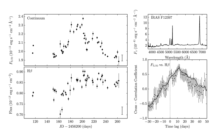
Figure 4: Results for IRAS F12397+3333 (same as Fig. 3).

Assuming first no reddening, we get $L_{5100}=3.9\times 10^{43}\rm erg~{}s^{-1}$. Using Eqn. 3 and our measured BH mass ($7.5\times 10^{6}M_{\odot}$) we get $\dot{m}_{{}_{\rm SS}}\simeq 1.3$. In the second case, $L_{5100}=1.69\times 10^{44}\rm erg~{}s^{-1}$ which results in $\dot{m}_{{}_{\rm SS}}\simeq 12.1$. The corresponding values for $\eta_{{}_{\rm SS}}=0.038$ are 0.5 and 4.6. All values are above or close the limiting case of $\dot{m}_{{}_{\rm SS}}=1$ and the ones corrected for reddening are the largest among all cases published so far in AGNs with directly measured BH mass. Comparing Eddington ratio estimations in other samples of NLS1s with estimates based on the virial method, e.g. the one shown in Figure 4 of Wang & Netzer 2003, we find that IRAS F12397+3333 and Mrk 142 have the highest Eddington ratios measured so far.

3.3 BH mass, Eddington rates, growth times and cosmological implications

As argued in numerous publications (e.g., Kelly et al. 2011 and references therein), understanding AGN variability is key to the understanding of the accretion mechanism, including the AD properties (Liu et al. 2008). Thus, the results of our monitoring campaign shed new light on several aspects of NLS1s in general and SEAMBHs in particular. First, we detected significant line and continuum variations, $\sim 15\%$, in three fast accreting black holes. Such variations have not been detected in most other known cases of NLS1s. The variations can provide important constraints on the properties of slim accretion disks (Mineshige et al 2000), a topic that we are currently investigating.

Second, all three objects are accreting close to or above the limit of $\dot{m}_{{}_{\rm SS}}\approx 1$ even under the most conservative estimate of $\eta_{{}_{\rm SS}}=0.038$. Two of the sources, Mrk 142 and IRAS F12397+3333, show the highest values of $\dot{m}_{{}_{\rm SS}}$ measured so far. They indicate physical conditions that are far outside the nominal conditions for thin SS type disks. Among reverberation-mapped AGNs, these are perhaps the best candidates for having slim accretion disks.

Third, the newly measured lag for Mrk 335 is smaller than the earlier measurements but still in reasonable agreement with the $R_{{}_{\rm BLR}}-L$ relation obtained by Bentz et al. (2013). This is not the case for Mrk 142, and for IRAS F12397+3333 assuming there is extinction along the line of sight to this source. Both these objects fall well below the above correlation. This leads to a suggestion that SEAMBHs may exhibit a somewhat different $R_{{}_{\rm BLR}}-L$ relationship. One possibility is that in such cases, the very different geometry of the slim disk results in a different radiation pattern. In particular, the face-on luminosity can be very large compared with the equatorial value leading to the possibility that equatorial BLR gas clouds are exposed to much weaker radiation than assumed in isotropic radiation fields, which affect their location. Such ideas have been around for some time (Netzer 1987; Korista, Ferland & Baldwin 1997; Netzer 2013) but have never been studied in relation to slim disks. In addition, the balance between gravity and radiation pressure force, which is proportional to $\dot{m}$, may affect BLR gas around slim disks in SEAMBHs more than in other AGNs. This can lead to marginally bound, or perhaps even unbound cloud systems (see discussion of these ideas in Marconi et al. 2008 and Netzer and Marziani 2010). If correct, the BH mass determination in such sources may be less secure. On the other hand, 7 of the sources with measured $\sigma_{*}$ studied by Woo et al (2013) are NLS1s and their virial-based BH mass is in reasonable agreement with the mass obtained by the $M_{\bullet}-\sigma_{*}$ relationship. Unfortunately none of the three sources studied here is included in the Woo et al. (2013) sample.

Fourth, the normalized accretion rates obtained here, at least for two of the cases, are so large that they must be important to the general issue of BH growth and BH duty cycle. In particular, in the exponential growth scenario, the growth time of massive BHs is inversely proportional to $\dot{m}$. Typical continuous growth times for local active BHs, based on typical Eddington rates of such sources ($\sim 0.1$), are of order the Salpeter time, $\sim 4\times 10^{8}$ yr (e.g., Netzer & Trakhtenbrot 2007). For the objects considered here, the growth time could be an order of magnitude or much shorter (see Netzer and Trakhtenbrot 2013 for similar considerations regarding growth times of SDSS AGNs).

Finally, the direct measurements of SEAMBH masses will allow us to estimate the cosmological distance to such objects using the relationship between the BH mass and the saturated luminosity of such objects (Wang et al. 2013). This can provide a new way to measure cosmological distances up to very high redshifts. We are extending the monitoring project to larger numbers and to higher redshifts in order to provide more precise calibration of this method.

4 Conclusions

We introduced the first results from a new project aimed at measuring accurate masses in AGNs hosting the fastest accreting active BHs. The first stage of the project includes 10 targets that were monitored with the Shangri-La telescope at the Lijiang station of the Yunnan observatory. The results pertain to three NLS1s for which we obtained detailed light curves and meaningful CCFs that can be used to derive accurate time lags and reliable BH masses. We find H$\beta$ time lags of $10.6_{-2.9}^{+1.7}$, $6.4_{-2.2}^{+0.8}$ and $11.4_{-1.9}^{+2.9}$ days for Mrk 335, Mrk 142 and IRAS F12397, respectively. For Mrk 142 and IRAS F12397 (assuming its continuum is extincted), the lags are shorter than expected from the most recent $R_{{}_{\rm BLR}}-L$ relationships for the general AGN population. The corresponding BH masses are $(8.3_{-3.2}^{+2.6})\times 10^{6}M_{\odot}$, $(3.4_{-1.2}^{+0.5})\times 10^{6}M_{\odot}$ and $(7.5_{-4.1}^{+4.3})\times 10^{6}M_{\odot}$ and the corresponding Eddington ratios ($\dot{m}_{{}_{\rm SS}}$) 1.6, 5.9 and 12.1 (extincted) or 1.3 (unextincted). All these values assume $\eta_{{}_{\rm SS}}=0.1$. Values of $\dot{m}$ as high as those measured for Mrk 142 and IRAS F12397 have never been directly measured in other AGNs. All three BHs are undergoing super-Eddington accretion with important consequences to the BH accretion mechanism, BH growth rate and, perhaps, cosmology.

Table 1: Basic data and variability amplitude

Object	$\alpha_{2000}$	$\delta_{2000}$	redshift	$E$(B-V)	monitoring period	$N_{\rm spec}$	variability amplitude($\%$)∗				Comparison stars
							$F_{\rm var}$(5100Å)	$F_{\rm var}$(V)	$F_{\rm var}({\rm H\beta}$)		$R_{*}$	P.A.
Mrk 335	00 06 19.5	+20 12 10	0.0258	0.030	2012 Oct$-$2013 Feb	91	5.2$\pm$0.5	3.9$\pm$0.3	3.4$\pm$0.3		$80^{\prime\prime}.7$	174.5∘
Mrk 142	10 25 31.3	+51 40 35	0.0449	0.015	2012 Nov$-$2013 Apr	119	8.1$\pm$0.6	5.5$\pm$0.4	7.8$\pm$0.5		$113^{\prime\prime}.1$	155.2∘
IRAS F12397+3333	12 42 10.6	+33 17 03	0.0435	0.017	2013 Jan$-$2013 May	51	5.6$\pm$0.6	3.2$\pm$0.4	4.5$\pm$0.6		$189^{\prime\prime}.0$	130.0∘

Note. — $E(B-V)$ is the Galactic extinction using the maps in Schlafly & Finkberiner (2011). $N_{\rm spec}$ is the number of spectroscopic observing epochs, $R_{*}$ is the angular distance to the target and P.A. is the position angle. ^∗Amplitudes were calculated using Eqn. 4. The uncertainties of $F_{\rm var}$ is calculated according to Edelson et al. (2002).

Table 2: Continuum and H$\beta$ light curves

Mrk 335				Mrk 142				IRAS F12397+3333
JD	$F_{5100}$	$F_{\rm H\beta}$		JD	$F_{5100}$	$F_{\rm H\beta}$		JD	$F_{5100}$	$F_{\rm H\beta}$
22.1913	$6.120\pm 0.118$	$5.904\pm 0.017$		37.4339	$1.552\pm 0.010$	$0.800\pm 0.007$		115.4571	$1.982\pm 0.009$	$0.789\pm 0.007$
23.3037	$6.478\pm 0.040$	$6.231\pm 0.033$		54.4214	$1.701\pm 0.010$	$0.798\pm 0.006$		116.4462	$2.069\pm 0.008$	$0.804\pm 0.006$
24.0274	$6.285\pm 0.023$	$6.002\pm 0.021$		55.4262	$1.811\pm 0.019$	$0.807\pm 0.008$		150.4556	$1.973\pm 0.017$	$0.820\pm 0.011$
25.0172	$6.056\pm 0.016$	$5.814\pm 0.017$		59.4444	$1.619\pm 0.012$	$0.825\pm 0.006$		151.4504	$1.936\pm 0.014$	$0.769\pm 0.010$
26.0242	$6.167\pm 0.021$	$5.797\pm 0.026$		60.4155	$1.631\pm 0.009$	$0.823\pm 0.008$		152.4339	$1.966\pm 0.022$	$0.813\pm 0.009$

Note. — The full version of this table is also available in machine-readable form in the electronic edition of the Astrophysical Journal. JD: Julian dates from 2456200; $F_{5100}$ and $F_{\rm H\beta}$ are fluxes at $(1+z)5100$Å  and H$\beta$ emission line in units of $10^{-15}\mathrm{~{}erg~{}s^{-1}~{}cm^{-2}~{}\AA^{-1}}$ and $10^{-13}\mathrm{~{}erg~{}s^{-1}~{}cm^{-2}}$, respectively. The systematic uncertainties of $F_{5100}$ and $F_{\rm H\beta}$ are ($\Delta F_{5100}$, $\Delta F_{\rm H\beta})=(0.138,0.091),(0.045,0.018)$ and $(0.035,0.018)$ for Mrk 335, Mrk 142 and IRAS F12397 respectively.

Table 3: Host galaxy decomposition

Object	Data set	Observational setup	$m_{\rm st}^{*}$	$R_{e}$	$n$	$b/a$	P.A.	Note	$\chi_{\nu}^{2}$
				(′′)			(deg)
Mrk 335	J9MU010	ACS, HRC, F550M	14.73					PSF	1.700
			17.78	0.09	0.89	0.04	44.45	Add’l PSF
			14.81	5.02	3.58	0.93	95.81	Elliptical
			-0.007					Sky
Mrk 142	IB5F010	WFC3, UVIS1, F547M	16.13					PSF	1.424
			18.27	0.41	0.45	0.78	14.25	Bulge
			16.34	4.73	[1.0]	0.56	39.53	Disk
			0.014					Sky
IRAS F12397	J96I090	ACS, HRC, F625W	16.27					PSF	1.630
			18.36	0.16	1.16	0.72	42.65	Nuclear Spiral?
			17.40	0.79	0.75	0.96	146.4	Bulge
			16.51	3.69	[1.0]	0.49	53.84	Disk
			0.007					Sky

Note. — The values in square brackets are fixed in the fitting procedure. *$m_{\rm st}$ is the ST magnitude, an $f_{\lambda}$-based magnitude system, $m_{\rm ST}=-2.5\log_{10}(f_{\lambda})-21.10$, for $f_{\lambda}$ in erg s^-1cm^-2Å^-1 (see Sirianni et al. 2005). The units of sky are electrons/s.

Table 4: Results of CCF analysis in rest frame of sources

	$F_{5100}{\rm~{}versus~{}H\beta}$
Object	$\tau_{\rm cent}$	$\tau_{\rm peak}$	$r_{\rm max}$
	(days)	(days)
Mrk 335	$10.6_{-2.9}^{+1.7}$	$8.2_{-1.1}^{+4.4}$	0.67
Mrk 142	$6.4_{-2.2}^{+0.8}$	$5.3_{-2.2}^{+2.6}$	0.68
IRAS F12397+3333	$11.4_{-1.9}^{+2.9}$	$11.9_{-2.2}^{+1.4}$	0.71

Table 5: Luminosity, BH mass and Eddington ratios

Object	FWHMa	$F_{\rm gal}^{b}$	$F_{\rm AGN}^{b}$	$L_{5100}$	$M_{\bullet}^{c}$	$\dot{m}_{{}_{\rm SS}}$
	(km s-1)	($10^{-15}~{}{\rm erg~{}s^{-1}~{}cm^{-2}~{}\AA^{-1}}$)		($10^{43}\rm erg~{}s^{-1})$	($10^{6}M_{\odot}$)	$\eta_{{}_{\rm SS}}=0.1$	$0.038$
Mrk 335	1997$\pm$265	0.99$\pm$0.10	5.20$\pm$0.37	4.9$\pm$0.4	$8.3_{-3.2}^{+2.6}$	1.6	0.6
Mrk 142	1647$\pm$ 69	0.37$\pm$0.04	1.27$\pm$0.15	3.7$\pm$0.4	$3.4_{-1.2}^{+0.5}$	5.9	2.3
IRAS F12397(I)	1835$\pm$473	0.65$\pm$0.06	1.44$\pm$0.14	16.9$\pm$1.7	$7.5_{-4.1}^{+4.3}$	12.1	4.6
IRAS F12397(II)	1835$\pm$473	0.65$\pm$0.06	1.44$\pm$0.14	3.9$\pm$0.4	$7.5_{-4.1}^{+4.3}$	1.3	0.5

Note. — IRAS F12397(I)/(II) mean with/without intrinsic reddening, respectively.

^aFWHM stands for $V_{\rm FWHM}$ in the text of the paper and is measured from the mean spectra.

^b$F_{\rm gal}$ and $F_{\rm AGN}$ are host galaxy and mean AGN fluxes at $(1+z)5100{\rm\AA}$. $F_{\rm gal}+F_{\rm AGN}=F_{\rm obs}$, where $F_{\rm obs}$ is the observed flux.

^c$M_{\bullet}$ are calculated using the centroid time lag, $V_{\rm FWHM}$ and $f_{\rm BLR}=1.0$. Uncertainties on $M_{\bullet}$ are the results of the errors on the time lags and the FWHMs. $L_{5100}$ is the mean AGN luminosity at rest-frame wavelength of 5100Å after the subtraction of the host galaxy contribution and allowing for Galactic extinction.

Table 6: Mrk 335: BLR size and continuum luminosity at different epochs

Epoch	$\tau_{\rm cent}$	$\tau_{\rm peak}$	$F_{\rm AGN}[5100{\rm\AA}(1+z)]$	$L_{5100}$	Reference
(JD2400000+)	(days)	(days)	(${\rm 10^{-15}~{}erg~{}s^{-1}~{}cm^{-2}~{}\AA^{-1}}$)	(${\rm 10^{43}erg~{}s^{-1}}$)
49156$-$49338	$16.8^{+4.8}_{-4.2}$	$18^{+5}_{-6}$	$6.12\pm 0.19$	$5.8\pm 0.2$	P04, B13
49889$-$50118	$12.5^{+6.6}_{-5.5}$	$13^{+9}_{-7}$	$7.25\pm 0.21$	$6.8\pm 0.2$	P04, B13
55440$-$55568	$14.3^{+0.7}_{-0.7}$	$14.0^{+0.9}_{-0.9}$	$5.84\pm 0.29$	$5.5\pm 0.3$	G12, B13
56222$-$56328	$10.6^{+1.7}_{-2.9}$	$8.2^{+4.4}_{-1.1}$	$5.20\pm 0.37$	$4.9\pm 0.4$	this paper

Note. — P04: Peterson et al. (2004); G12: Grier et al. (2012); B13: Bentz et al. (2013)

References

- (1) Abramowicz, M. et al. 1988, ApJ, 332, 646
- (2) Ade, P. A. R. et al. 2013, A&A, in press (arXiv:1303.5076)
- (3) Ai, Y. et al. 2013, AJ, 145, 90
- (4) Alexander, T. 1997, in Astronomical Time Series, ed. D. Maoz, A. Sternberg, & E. M. Leibowitz (Dordrecht: Kluwer), 163
- (5) Arévalo, P., McHardy, I. M. & Summnons, D. P. 2008, MNRAS, 388, 211
- (6) Atlee, D. W. & Mathur, S. 2009, ApJ, 703, 1597
- (7) Bahcall, J. N., Kozlovsky, B. Z. & Salpeter, E. E. 1972, ApJ, 171, 467
- (8) Bardeen, J. M., Press, W. H. & Teukolsky, S. A. 1972, ApJ, 178, 347
- (9) Bentz, M. et al. 2009a, ApJ, 697, 160
- (10) Bentz, M. et al. 2009b, ApJ, 705, 199
- (11) Bentz, M. et al. 2013, ApJ, 767, 149
- (12) Bianchi, S. et al. 2009, A&A, 495, 421
- (13) Blandford, R. D. & McKee, C. F., 1982, ApJ, 255, 419
- (14) Brightman, M. et al. 2013, MNRAS, 433, 2485
- (15) Collin, S. et al. 2002, A&A, 388, 771
- (16) Davis, S. & Laor, A. 2011, ApJ, 728, 98
- (17) Denney, K. et al. 2010, ApJ, 721, 715
- (18) Denney, K. et al. 2013, ApJ, 775, 60
- (19) Edelson, R. A. & Krolik, J. H. 1988, ApJ, 333, 646
- (20) Edelson, R. A. et al. 2002, ApJ, 568, 610
- (21) Elvis, M. et al. 1994, ApJS, 95, 1
- (22) Elvis, M. et al. 2012, ApJ, 759, 6
- (23) Ferrarese, L. et al. 2001, ApJ, 555, L79
- (24) Hook, I. M., 2012, IAUS, 285, 63
- (25) Hu, C., Wang, J.-M., Ho, L. C. et al. 2008, ApJ, 687, 78
- (26) Gaskell, C. M. & Peterson, B. M. 1986, ApJS, 65, 1
- (27) Gaskell, C. M. & Sparke, L. S. 1986, ApJ, 305, 175
- (28) Giannuzzo, M. Z. & Stirpe, G. M. 1996, A&A, 314, 419
- (29) Giannuzzo, M. Z. et al. 1998, A&A, 330, 894
- (30) Grier, J. A. et al. 2012, ApJ, 755, 60
- (31) Grupe, D., Wills, B. J., Wills, D. & Beuermann, K. 1998, A&A, 333, 827
- (32) Grupe, D. et al. 2001, A&A, 367, 470
- (33) Kaspi, S. et al. 2000, ApJ, 533, 631
- (34) Kaspi, S. et al. 2005, ApJ, 629, 61
- (35) Kaspi, S. et al. 2007, ApJ, 659, 997
- (36) Kassebaum, T. M. et al. 1997, ApJ, 475, 106
- (37) Keel, W. C., de Grijp, M. & Miley, G. K. 1988, A&A, 203, 250
- (38) Kelly, B. C., Sobolewska, M. & Siemiginowska, A. 2011, ApJ, 730, 52
- (39) Kelly, B. C. & Shen, Y. 2013, ApJ, 764, 45
- (40) Kim, M. et al. 2008, ApJS, 179, 283
- (41) Kinney, A. L. et al. 1996, ApJ, 467, 38
- (42) Klimek, E. S., Gaskell, C. M. & Hedrick, C. H., 2004, ApJ, 609, 69
- (43) Kobayashi, C. & Nomoto, K. 2009, ApJ, 707, 1466
- (44) Korista, K., Ferland, G. & Baldwin, J. 1997, ApJ, 487, 555
- (45) Krist, J. 1993, in ASP Conf. Ser. 52, Astronomical Data Analysis Software and Systems II, ed. R. J. Hanisch, R. J. V. Brissenden, and J. Barnes (San Francisco, CA: ASP), 536
- (46) Krist, J. 2003, ACS Instrument Science Report (ISR 2003-06; Baltimore, MD: STScI)
- (47) Laor, A. & Netzer, H. 1989, MNRAS, 238, 897
- (48) Liu, H.-T., Bai, J.-M., Zhao, X.-H. & Ma, L. 2008, ApJ, 677, 884
- (49) McLure, R. J. & Dunlop, J. S. 2004, MNRAS, 352, 1390
- (50) Maoz, D., et al. 1990, ApJ, 351, 75
- (51) Marconi, A. et al. 2004, MNRAS, 351, 169
- (52) Marconi, A. et al. 2008, ApJ, 678, 693
- (53) Mathur, S. et al. 2012, ApJ, 754, 146
- (54) Mineshige, S. et al. 2000, PASJ, 52, 499
- (55) Netzer, H. 1987, MNRAS, 225, 55
- (56) Netzer, H. 1990, Saas-Fee Advanced Course of the Swiss Society for Astrophysics and Astronomy: Active Galactic Nuclei, p. 57 - 160
- (57) Netzer, H. 2013, Physics and Evolution of Active Galactic Nuclei, Cambridge University Press.
- (58) Netzer, H. & Marziani, P. 2010, ApJ, 724, 318
- (59) Netzer, H. & Peterson, B. M. 1997, Astronomical Time Series, Eds. D. Maoz, A. Sternberg, and E.M. Leibowitz, 1997 (Dordrecht: Kluwer), p. 85.
- (60) Netzer, H. & Trakhtenbrot, B., 2013 (submitted to MNRAS)
- (61) Netzer, H. et al. 2007, ApJ, 671, 1256
- (62) Netzer, H. & Trakhtenbrot, B. 2007, ApJ, 654, 754
- (63) Onken, C. et al. 2004, ApJ, 615, 645
- (64) Park, D. et al. 2012, ApJ, 747, 30
- (65) Peng, C. Y. et al. 2002, AJ, 124, 266
- (66) Peng, C. Y. et al. 2010, AJ, 139, 2097
- (67) Peterson, B. M. 1993, PASP, 105, 247
- (68) Peterson, B. M. 2013, SSRv, tmp..60p
- (69) Peterson, B. M. et al. 1998, ApJ, 501, 82
- (70) Peterson, B. M. et al. 2004, ApJ, 613, 682
- (71) Richards, G. et al. 2006, ApJS, 166, 470
- (72) Risaliti, G. Young, M. & Elvis, M. 2009, ApJ, 700, L6
- (73) Rodríguez-Pascual, P. M. et al. 1997, ApJS, 110, 9
- (74) Schlafly, E. F. & Finkbeiner, D. P. 2011, ApJ, 737, 103
- (75) Shakura, N. I. & Sunyaev, R. 1973, A&A, 24, 337
- (76) Shemmer, O. & Netzer, H. 2000, arXiv:astro-ph/0005163
- (77) Shemmer, O. et al. 2006, ApJ, 646, L29
- (78) Shen, Y. 2009, ApJ, 704, 89
- (79) Sirianni, M. et al. 2005, PASP, 117, 1049
- (80) Trakhtenbrot, B. & Netzer, H., 2012, MNRAS, 427, 3081
- (81) Vanden Berk, D. E. et al. 2001, AJ, 122, 549
- (82) Vestergaard, M. & Osmer, P. S. 2009, ApJ, 699, 800
- (83) Wang, J.-M. & Zhou, Y.-Y. 1999a, ApJ, 516, 420
- (84) Wang, J.-M., Szuszkiewicz, E., Lu, F.-J. & Zhou, Y-.Y. 1999b, ApJ, 522, 839
- (85) Wang, J.-M. & Netzer, H. 2003, A&A, 398, 927
- (86) Wang, J.-M., Watarai, K.-Y. & Mineshige, S. 2004, ApJ, 607, L107
- (87) Wang, J.-M., Chen, Y.-M. & Zhang, F. 2006, ApJ, 647, L17
- (88) Wang, J.-M., Hu, C. et al. 2009, ApJ, 697, L141
- (89) Wang, J.-M., Du, P., Valls-Gabaud, D., Hu, C. & Netzer, H., 2013, Phy. Rev. Lett., 110, 081301
- (90) Woo, J.-H. et al. 2010, ApJ, 716, 269
- (91) Woo, J.-H. et al. 2013, ApJ, 772, 49
- (92) Yip, C. W. et al. 2009, AJ, 137, 5120
- (93) Zhou, X.-L. & Zhang, S.-N. 2010, ApJ, 713, L11
- (94) Zu, Y. et al. 2011, ApJ, 735, 80
- (95) Zuo, W.-W. et al. 2012, ApJ, 758, 104