Collective effects in vortex movements in complex (dusty) plasmas

Abstract

We study the onset and characteristics of vortices in complex (dusty) plasmas using two-dimensional simulations in a setup modeled after the PK-3 Plus laboratory. A small number of microparticles initially self-arranges in a monolayer around the void. As additional particles are introduced, an extended system of vortices develops due to a non-zero curl of the plasma forces. We demonstrate a shear-thinning effect in the vortices. Velocity structure functions and the energy and enstrophy spectra show that vortex flow turbulence is present that is in essence of the “classical” Kolmogorov type.

Introduction—Complex plasmas consist of micrometer-sized particles embedded in a low temperature plasma. Experimenters can record the trajectories of the microparticles with digital cameras and study the microparticle behavior in detail. Complex plasmas are ideal model systems for nano fluids, phase transitions, transport processes, etc Morfill and Ivlev (2009). They display many collective effects. For instance, vortices in which the microparticles move in circles are common. They appear when gravity is compensated by thermophoresis Morfill et al. (2004); Rubin-Zuzic et al. (2007); Schwabe et al. (2009) and in weightless systems Morfill et al. (1999); Fortov et al. (2003); Nefedov et al. (2003) and can be induced externally, for instance by a laser Klindworth et al. (2000); Miksch and Melzer (2007), by a probe Law et al. (1998); Uchida et al. (2009), or by gas flow Vladimirov et al. (2001); Mitic et al. (2008); Schwabe et al. (2011); Fink et al. (2013). Vortices can convoy nucleation Nosenko et al. (2007) and lead to shear flow instabilities at their edges Heidemann et al. (2011). The origin of self-excited vortices in complex plasmas has long been a topic of discussion. They could be induced by the microparticle size dispersion Rubin-Zuzic et al. (2007); Yokota and Honda (1996), charge gradients Vaulina et al. (2000, 2003), the void Mamun and Shukla (2004), or a non-zero curl of the forces that the plasma exerts on the microparticles Akdim and Goedheer (2003); Goedheer and Akdim (2003).

As we show in the following, vortices in complex plasmas are an ideal test-bed for studying the onset of turbulence and collective effects on the microcanonical level Morfill et al. (2004). The description and dynamics of a turbulent complex plasma is an outstanding problem. Turbulence can be present in the background gas Robertson and Sternovsky (2007); Schwabe et al. (2011) or plasma Klinger et al. (2001); Benkadda and Tsytovich (2002) or induced by instabilities or waves in the dusty plasma itself Shukla et al. (2004); Pramanik et al. (2003); Tsai et al. (2012). In comparison with traditional experiments on turbulence (see, e.g., Lewis and Swinney (1999); Arnèodo et al. (2008); Monchaux (2012)), the particles that transmit the interaction can be visualized directly. Still many physical questions remain unanswered partly because the adequate simulations are lacking. Simulations help identify relevant experimental parameters and lead the way to designing related experiments.

Hybrid simulations are especially well suited to study self-excited vortices. In these simulations, the plasma is typically simulated as a fluid and coupled with a separate simulation of the microparticle dynamics. This allows taking into account the forces that the plasma exerts on the microparticles and letting vortices develop naturally. Then, the reason for the self-excitation of vortices and the exact process of the onset of vortices can be determined.

Here, we present two-dimensional simulations of vortices in complex plasmas to investigate the onset of turbulence and collective effects. We model the discharge plasma and the cooperative dynamics of the microparticles embedded in it and demonstrate that the microparticle shear flow is relevant to that observed experimentally, and subjected to shear-thinning and turbulence.

Simulation particulars—We use the simulation setup described in Schwabe and Graves (2013), which is a two-dimensional model of the central plane of the PK-3 Plus chamber Thomas et al. (2008). It consists of a hybrid fluid-analytical description of the plasma by Kawamura et al. (2011), coupled to a molecular-dynamics (MD) simulation of the microparticle dynamics. The MD simulation is based on the Large-scale Atomic/Molecular Massively Parallel Simulator (LAMMPS) Plimpton (1995), modified to take into account the plasma forces. The microparticles interact via Yukawa pair potentials and are subject to random forces mimicking interactions with background atoms bumping into them. There is also a background friction force exerted by the neutral gas on the microparticles, the so-called Epstein drag force Epstein (1924). The ion flux and ambipolar electric field from the plasma simulation are used to calculate the ion drag and confinement forces acting on the microparticles. A naturally occurring non-vanishing curl of the sum of these forces leads to the generation of vortices.

For the simulations presented here, we use argon at a pressure of 10 Pa as buffer gas. The microparticles have a diameter of 3.4 $\mu$m, a mass of $3.1\times 10^{-14}$ kg, and a charge of -3481 e. The friction constant with the background gas is $\gamma_{\text{Ep}}=37\,\text{s}^{-1}$. The electron temperature is 2.4 eV, the ion and neutral gas temperatures 300 K. The mean electron and ion number densities are $3.4\times 10^{14}\,\text{m}^{-3}$, with a maximum in the center of the simulation box (see Schwabe and Graves (2013)). We do not take into account the effect of the microparticles on the plasma. Unless otherwise mentioned, we used 7100 particles in the simulations runs presented here. The areal density of the cloud is $1.4\times 10^{7}\,\text{m}^{-2}$.

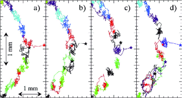
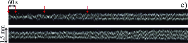
Figure 1: (color online) (a-d) Trajectories that show the process of adding single particles to a monolayer. The trajectories of individual particles are distinguished by color. The start point of each trajectory is indicated by a star. e) Space-time plot (periodgram) that demonstrates the development of the width of the central part of the microparticle cloud with time. To make this picture, we added the pixel intensities of images showing the particle positions in the region $y=9.5-10.5$ mm as a function of $x$ position for frames corresponding to a total of 50 particle injections and plot the resulting graphs next to each other. In the periodgram, the vertical axis corresponds to $x$-position, and the horizontal axis to time. Injections occur every minute. The arrows indicate the injections a)-d).

Onset of vortices—We mimic the experimental injection process by placing microparticles near the sheath edge. They are then pushed into the plasma by the ambipolar electric field. Inside the plasma bulk, the ion drag force drives the microparticles around the void, where they arrange in a monolayer along the equilibrium line where the counteracting ion drag and ambipolar electric force are balanced. Figure 1 shows trajectories of particles inside this monolayer as progressively more particles are added. A single particle added to the monolayer rapidly finds a place inside (Fig. 1(a)). The next added particle is also incorporated into the monolayer, but the propagation of forces along the monolayer leads to a particle further down (shown in light green) being ejected from the layer. The ejected particle hops along the inside of the monolayer (Fig. 1(b)). The next particles that are injected disturb the layer, causing transverse displacement of other particles, but no vortices appear yet (Fig. 1(c)). Two layers of particles form, and vortex motion ensues only after the 12th particle injection (Fig. 1(d)). The space-time plot (periodgram) (Fig. 1(e)) demonstrates the growth of the cloud width with additional injections of single particles. An additional particle is injected every 60 s.

Figure 2: (color online) (top) The sum of the ion drag $F_{i}$ and electric force $F_{e}$ acting on the particles (vectors, color online, right color map) overlaid a map of the curl of the force field (greyscale, left color map). The equilibrium line is clearly visible in the vector field. The edge of the cloud in the curl map is enhanced, which is an artefact of the way curl F was calculated. (bottom) Map of the absolute value of the curl of the force field. Both curl maps uses a threshold of $\pm 5\times 10^{-12}$ N/m to enhance the contrast.

Figure 2 shows the vector plot of the combined plasma forces acting on the particles, the ion drag force $F_{i}$ and the ambipolar electric force $F_{e}$. There is a single line around the void at which the sum of these two forces vanishes. This equilibrium line is visible in Fig. 2 as the line to which the vectors point. On the outside of the equilibrium line, the confining ambipolar electric force dominates, whereas on the inside of the equilibrium line, the ion drag force dominates, keeping the central ’void’ particle-free. The cause of the finite width of the microparticle cloud is the mutual interparticle repulsion.

The gray-scaled background of Fig. 2 maps the non-zero component of the curl of the plasma force field, $\nabla\times({\bf F_{i}}+{\bf F_{e}})$ footnote1 . The magnitude of the curl of the vector field is largest near the edges of the microparticle cloud, on the outside of the equilibrium line, whereas it nearly vanishes on the inside of the equilibrium line and in the mid-plane of the simulation box. This qualitatively confirms the basic result of Akdim and Goedheer (2003): The vortices can be caused by a non-vanishing curl of the plasma force (see also footnote2 ).

Fully developed system of vortices—Once several layers of microparticles are present, the vortices are fully developed. Figure 3 visualizes the movement of microparticles inside a cloud with two vortices. The particles move towards the simulation box center along the outside of the cloud and back towards the cloud edge in the central plane, as in the experiments in the PK-3 Plus laboratory on board the International Space Station footnote3 .

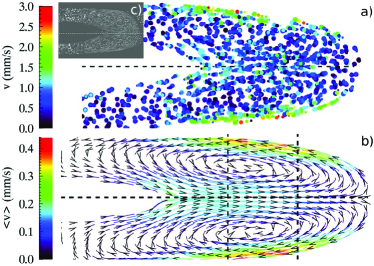
Figure 3: (color online) Simulated (a,b) and experimental vortices (c). The horizontal dashed lines mark the chamber midplane/simulation box center. The field of view is (a,b) $23\times 10$ mm² and (c) $30\times 20$ mm². a) Positions of 1/10 of all particles in the simulation. The dots indicate four particle positions 0.2 s apart for each particle and grow with time. The color of the dots indicates the total particle velocity, which is shown with a threshold of 3 mm/s. b) Streamlines and arrows indicate the mean velocity field of the simulated vortices. The mean was calculated by averaging over at least five particles for each position. The vertical dashed lines indicate the position of the sliding window used for Fig. 5. c) Overlay of 60 pictures (30 s) taken with the PK-3 Plus laboratory, courtesy of the PK-3 Plus team Thomas et al. (2008). The images are mirrored horizontally to correspond to the simulation.

The particles move fastest at the edge of the vortices, where the rotational energy is concentrated, see Fig. 4 showing the enstrophy density of system. We calculate the enstrophy density following Heidemann et al. (2011): Firstly, we determine the 16 closest neighbors of every particle $i$ and find the vectors to their positions $\bf{r_{ij}}=\bf{r_{j}}-\bf{r_{i}}$ and the relative velocities $\bf{v_{ij}}=\bf{v_{j}}-\bf{v_{i}}$. The vorticity $\omega_{i}$ is a function of the projections $c_{ij}$ of the relative velocity onto the vectors orthogonal to $\bf{r_{ij}}$:

$$\omega_{i}={\bf e_{z}}\cdot(\text{\bf curl}\,{\bf v})_{i}=\frac{1}{nn}\sum_{j=1}^{nn}c_{ij},$$ (1)

where $nn=16$ is the number of neighbors used in the calculation, $\bf{e_{z}}=\bf{e_{x}}\times\bf{e_{y}}$ is the unit vector in direction perpendicular to the plane of the simulation, and $c_{ij}=({\bf e_{z}}\times{\bf r_{ij}})\cdot{\bf v_{ij}}/r_{ij}^{2}$. Finally, we calculate the enstrophy density $\Omega_{kl}$ in every grid cell (k,l) from the average squared vorticity

$$\Omega_{kl}=\left(\frac{1}{n}\sum_{i=0}^{n}\omega_{i}\right)^{2},$$ (2)

where n is the number of particles in the cell.

Figure 4: (color online) Enstrophy density $\Omega$ of the vortices. Field of view: $23\times 12\,\text{mm}^{2}$.

Figure 4 shows that the enstrophy density is concentrated at the edges of the microparticle cloud, where the microparticles move the fastest. As there are considerable velocity differences across the cloud, we shall next see whether the vortices produce any shear stress.

Shear thinning—We follow Nosenko et al. (2013) to calculate the shear stress $\sigma_{xy}$, i.e., the off-diagonal elements of the pressure tensor, that is build up from the contributions of each particle’s neighbors, neglecting the kinetic component. For a two-dimensional system in polar coordinates, $\sigma_{xy}$ is given by

$$\sigma_{xy}=-\frac{1}{2}n^{2}\int_{0}^{r_{max}}dr\,r^{2}\frac{dV}{dr}\int_{0}^{2\pi}d\phi\cos\phi\sin\phi\,g(r,\phi),$$ (3)

where $n$ is the number density of the microparticles, $V$ is the Yukawa potential, and $g(r,\phi)$ is the radial pair distribution function. The insets (a) and (b) in Fig. 5 show the pair correlation functions at the upper and lower edges of the cloud. As in Nosenko et al. (2013), the elliptical distortion of $g(r,\phi)$ shows strong shear stress.

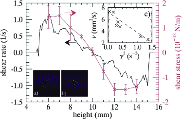
Figure 5: (color online) Shear rate and shear stress as a function of height above the lower sheath edge. Insets: Radial pair correlation functions at the lower (a) and upper (b) edges of the cloud, c) viscosity $\nu$ as a function of squared shear stress $\gamma^{2}$, demonstrating shear thinning. The dashed line is a guide to the eye.

The main part of Fig. 5 shows the shear rate $\gamma=(\partial v_{x}/\partial y)+(\partial v_{y}/\partial x)$, calculated from the velocity maps, and the shear stress $\sigma_{xy}$ as a function of height above the lower sheath edge in a sliding window of size $5\times 2\,\text{mm}^{2}$ at a horizontal distance of 12 mm from the plasma center (see Fig. 3). The vertical center of the simulation box is at a height of 10 mm. Both the shear rate and the shear stress vanish in the middle, where all particles are moving towards the edge of the cloud. Their absolute values are largest close to the area where the opposite fluxes induced by the vortices meet, as expected. Numerically, the values are close to those found in experiments by Nosenko et al. (2013), in which laser-induced motion of microparticles is studied. We also observe shear-thinning, as can be seen in Fig. 5(c) footnote4 : The viscosity $\nu=\sigma_{xy}/(\rho\gamma)$, with $\rho$ being the areal mass density, decreases as a function of squared shear stress.

Flow velocity—The parameters of the simulated vortex flow fit real experiments performed with complex plasmas. For instance, using a mean viscosity of $\nu=5\,\text{mm}^{2}\text{/s}$, a flow velocity of $v=2\,\text{mm/s}$ and a typical size of the vortices of $L=10\,\text{mm}$ (see Figs. 3,5), we obtain a Reynolds number $\mathcal{R}=vL/\nu\sim 4$, which is well in-line with observations Morfill et al. (2004); Heidemann et al. (2011). At such a low value, e.g., water flow is typically laminar. Nevertheless, we do find evidence that turbulence is present in the system of vortices, as we shall see next.

Turbulence—The origin of the turbulent pulsations in our simulations is twofold. It is the external normally-distributed random forces and the mutual interparticle interactions leading to randomization as well. Speaking about turbulence, first of all it is necessary to scale the fluctuations. Using the average viscosity $\nu=5\,\text{mm}^{2}/\text{s}$ and the mean enstrophy density of $\Omega=0.4\,\text{s}^{-2}$ obtained in simulations, we get an energy dissipation rate per unit mass Frisch (1995) of the order of $\epsilon=2\nu\Omega=4\,\text{mm}^{2}/\text{s}^{3}$. This results in a Kolmogorov length scale of $L_{K}=\left(\nu^{3}/\epsilon\right)^{1/4}=2.4\,\text{mm}$, which is an intermediate scale between the size of the simulation box ($20\times 45\,\text{mm}^{2}$) and the interparticle distance ($0.15\,$mm).

Traditionally, the scaling of vortices is studied by computing structure functions. The longitudinal structure functions of order $p$, $S_{p}(r)$, are given by

$$S_{p}(r)=\left<(\Delta u_{r})^{p}\right>=\left<[u(x+r)-u(x)]^{p}\right>,$$ (4)

where $u(x)$ is the velocity component parallel to the relative displacement r. We use the absolute value of the velocity difference in the calculations, as this is more numerically stable and does not significantly change the results Lewis and Swinney (1999). For fully developed turbulence, the structure functions show a power law scaling Frisch (1995)

$$S_{p}\propto r^{\zeta_{p}}.$$ (5)

Kolmogorov (1941) predicted the exponents to be given by $\zeta_{p}=p/3$. Figure 6 shows the horizontal velocity structure functions measured in the region to the right of the void, where the particles are flowing mainly in horizontal direction. As recommended by Lewis and Swinney (1999), we use extended self-similarity Benzi et al. (1993), i.e., we plot $S_{p}$ vs. $S_{3}$ on a log-log plot and use the fact that $\zeta_{3}=1$ according to Kolmogorov’s theory. The slopes of the plots are then given by $\zeta_{p}/\zeta_{3}=\zeta_{p}$. Figure 6 shows that the slopes are very close to those predicted by Kolmogorov (as the overplotted solid lines in the figure indicate).

Figure 6: (color online) Squares: First (p=1) through sixth (p=6) order longitudinal velocity structure functions $S_{p}$ as a function of the third order structure function $S_{3}$. The lines are those predicted by classical Kolmogorov theory $S_{p}\propto r^{\zeta_{p}}$, with $\zeta_{p}=p/3$. Inset: Energy (bottom) and Enstrophy density spectrum (top). The slopes of the lines overplotted on the energy spectrum are -3 and -5/3.

The inset in Fig. 6 shows the energy and enstrophy density spectra. The energy spectrum is calculated from the sum of the squares of the Fourier transformed velocity maps (see Fig. 3), the enstrophy spectrum from the enstrophy map (see Fig. 4). The two lines that are overplotted on the energy spectrum have the slopes -3 and -5/3, as expected: The $\propto k^{-5/3}$ dependence is typical inside the inertial range, and the cross-over to $\propto k^{-3}$ is due to friction Frisch (1995).

Summary—To conclude, we numerically studied two-dimensional vortices in a complex plasma. We showed how these vortices develop from a monolayer around the void, and that a non-zero curl of the combined ion drag and electric forces causes the vortex movement of the microparticles. We then investigated the properties of fully developed system of vortices, for instance the flow field and shear stress. In particular, we showed that turbulence is present in the flow induced by the vortices and demonstrated that the velocity structure functions scale very close to the predictions by Kolmogorov theory. These results show that it should be possible to use common experimental situations like vortices in complex plasmas to study turbulence on the level of individual particles.