Adaptive input design for LTI systems^⋆

Abstract

Optimal input design for parameter estimation has obtained extensive coverage in the past. A key problem here is that the optimal input depends on some unknown system parameters that are to be identified. Adaptive design is one of the fundamental routes to handle this problem. Although there exist a rich collection of results on this problem, there are few results that address dynamical systems. This paper presents sufficient conditions for convergence/consistency and asymptotic optimality for a class of adaptive systems consisting of a recursive prediction error estimator and an input generator depending on the time-varying parameter estimates. The results apply to a general family of single input single output linear time-invariant systems. An important application is adaptive input design for which the results imply that, asymptotically in the sample size, an adaptive scheme recovers the same accuracy as the off-line prediction error method that uses data from an experiment where perfect knowledge of the system has been used to design an optimal input spectrum.

I Introduction

With the rapid developments in model based engineering, compare with the petrochemical industry where it is reported that all plants employ model predictive control, the high cost of modeling is coming more and more into focus as a limiting factor [79]. Often the only practical means to modeling is data-driven modeling, i.e. system identification. For this type of modeling, the major part of the cost is associated with performing experiments on the plant in question. A key variable here is the duration of the experiments since it strongly couples to costs in terms of personell, energy, material and production losses.

For dynamical systems it has been shown that careful design of the experiment can lead to quite drastic reduction in the required experimental time as compared to standard white noise excitation or step testing [7, 80]. It has also been stressed that the experimental conditions are essential for making system identification robust with respect to many of the design variables that are involved, e.g. model structure and orders, and with respect to the resulting end performance [36].

The aforementioned observations have prompted renewed interest in optimal experiment design – a topic that has been studied extensively over the past century, see, e.g., [4], [5], [10], [19], [31], [57], [68], [78] and references therein. Recent advances include novel computationally tractable algorithms [40], least-costly and application oriented frameworks [11, 36], closed-loop methods [34, 33, 69, 60, 49], and extensions to non-linear models [77, 21, 17].

A key problem in optimal experiment design is that the optimal experiment typically depends on the system parameters that are to be identified. One of the fundamental routes to cope with this problem is to employ adaptive schemes, meaning that as information from the system is gathered the experimental conditions are changed. Adaptive design is usually called sequential design in the statistics literature, where there exist a rich collection of results and applications (see, e.g., [46] and the references therein).

When only the input excitation is considered part of the experiment design, we will use the terminology input design. Adaptive input design has been studied in many works in engineering literature (see, e.g., [51], [66], [72], [27], [28] and [39]). However, as pointed out in [35] and [28], there are few results that address this problem for dynamical systems. Given the increasing practical relevance of input design, it is becoming urgent to provide a solid theoretical foundation for such methods.

When the system is linear time-invariant and belongs to the model set, and the input is (quasi-)stationary, it is only the second order properties of the input that asymptotically (in the sample size) influence the model quality. Thus in this case it is the spectrum, or equivalently the autocorrelation sequence, of the input that is the design variable in optimal input design. The actual input sequence can be generated by filtering white noise through an input spectrum shaping filter corresponding to a stable spectral factor of the optimal input spectrum [40]. Building on this, an obvious approach to adaptive input design is to combine a recursive identification scheme with a time-varying input spectrum shaping filter, computed from the solution of the optimal input design problem using the the most recent model estimate as a substitute for the true system.

Such a certainty equivalence approach leads to an adaptive feedback system where, similar to adaptive control, the input properties change over time depending on the response of the system. From a performance perspective there are several issues that are non-trivial to analyze:

• Under which conditions will the parameter estimates of such a procedure converge?

• If the algorithm converges, will it be consistent, i.e. will the model parameters correspond to the true system parameters?

• If the algorithm converges to a correct system description, how does the resulting (large sample) accuracy compare to the accuracy an oracle, having access to the unknown true parameters for the experiment design already at the beginning of the experiment, could achieve?

In regards to (iii), notice that even if the parameters converge to the true values so that, as the experiment time progresses towards infinity, the input behaves closer and closer to a stationary signal having the optimal spectrum, suboptimal experimental conditions prevail in the meantime and it is not evident that the algorithm is able to catch up with the loss of accuracy this causes – this strongly depends on the rate of convergence of the algorithm.

An early version of the above concept was presented in [51]. A severe limitation was that the parameter estimation was not recursive, requiring re-identification using all past data for each new measurement. Furthermore, no statistical analysis was provided and even if, for this off-line algorithm, (i) and (ii) can be dealt with rather straightforwardly using results from [53], (iii) is non-trivial to analyze since the input signal is non-stationary.

Subsequently, the recursive certainty equivalence approach adopted in this contribution was outlined in [27], but without formal treatment of (i)–(iii). Recently, [28] takes a different approach and focus on a smaller class of problems, namely, identification of ARX systems with input filter of finite impulse response (FIR) type as in [51]. The advantage of using ARX-models is that the analysis of the recursive least-squares method can be carried out with a powerful result in [47].

There exists an extensive body of literature on general recursive stochastic algorithms, e.g. [52, 45, 56, 13, 15, 25, 26, 14]. Building on this work, the objective of this paper is to strengthen the theoretical foundations of the adaptive input design framework outlined in [27], providing results for (i)–(iii), hereby validating current practice in input design.

While we will cover (i) and (ii), our primary objective will be to deal with (iii). In particular, with $\theta^{\ast}$, $\theta_{n}$ and $\theta_{n}^{\ast}$ denoting the true parameter vector, the parameter estimate in the adaptive algorithm, and the off-line parameter estimate obtained from an experiment using the optimal input, respectively, we will be interested in establishing conditions for when adaptive input design asymptotically yields the same asymptotic accuracy as the optimal non-adaptive design in the sense that

$$\sqrt{n}(\theta_{n}-\theta^{\ast})$$

and

$$\sqrt{n}(\theta_{n}^{\ast}-\theta^{\ast})$$

have the same asymptotic distribution. A pre-requisite for this is (of course) that the recursive estimation algorithm is able to achieve this when the optimal input is used. Another ambition has been to cover the general class of single-input single-output (SISO) linear time-invariant (LTI) systems and associated model structures considered in [54]. The recursive prediction error (RPE) approach [52, 56] fulfills these objectives. However, this algorithm requires a projection mechanism and one generally cannot exclude the possibility that the sequence of estimates gets trapped at the boundary where the projection takes place. In the closely related approach [25, 26], the projection is replaced by a resetting mechanism which allows almost sure convergence to the true parameter vector to be established. A restrictive assumption here is that the asymptotic prediction error criterion is only allowed to have the true parameter vector as stationary point. This is a more severe conditition than identifiability. However, for a method that, as in the case of RPE, is based on gradient based non-linear search the best one can hope for is that convergence takes place to the set of stationary points. Notice that the corresponding off-line result [53], which proves convergence to the global minimum, makes the assumption that the global minimum can be found - something that is not easy to guarantee in practice using gradient based methods, being on-line or off-line. However, as our focus is (iii), which has convergence to the true system parameters as a pre-requisite, we have chosen to base our algorithm and analysis on the work [25, 26], thus avoiding the issue of clustering at the boundary. Recently, a novel recursive algorithm for ARMAX models has been proposed in [14] for which a powerful convergence result has been established. Unfortunately, for our considerations, this convergence result applies only when the input is white and, furthermore, the asymptotic accuracy of this algorithm is not known, and hence, at least at present, this algorithm is not suited to our purpose.

The paper starts off in Section II by introducing the system and model assumptions, together with the input signal generation mechanism that will be employed. The latter depends on the estimated parameter vector. Prediction error identification is discussed in Section III, leading up to the presentation of the complete adaptive algorithm, comprising the true system, the recursive estimation algorithm and the input generator, at the end of the section. Formal results on convergence/consistency and asymptotic distribution for the adaptive system are provided in Section IV. These results are quite general in that they make no specific use of the functional relationship between the parameter estimate and the input generator, other than that this is a sufficiently smooth map. These results are then placed in the context of adaptive input design in the following Section V, where a complete adaptive input design algorithm is presented, together with the result that this algorithm achieves the same asymptotic accuracy as an oracle. The algorithm is illustrated on a numerical example in Section VI. Conclusions are provided in Section VII. Proofs are provided in the appendices.

Notation: Throughout the paper, unless otherwise specified, we will employ the following notation. Our problem will be embedded in an underlying complete probability space $(\Omega,{\mathcal{F}},{\mathbb{P}})$, where $\Omega$ is the sample space, ${\mathcal{F}}$ is the $\sigma$-algebra that defines events $E$ in $\Omega$ which are measurable, i.e., for which the probability ${\mathbb{P}}(E)$ is defined. Let ${\mathbb{E}}[\cdot]$ be the expectation operator with respect to the probability measure. If $A$ is a vector or matrix, its transpose is denoted by $A^{T}$. If $P$ is a square matrix, $P>0$ ($P<0$) means that $P$ is a symmetric positive (negative) definite matrix of appropriate dimensions while $P\geq 0$ ($P\leq 0$) is a symmetric positive (negative) semidefinite matrix. If the square matrix $P$ is nonsingular, its inverse is denoted by $P^{-1}$. $I_{m}$ stands for the identity matrix of order $m$, $0_{m\times n}$ stands for the zero matrix of dimensions $m\times n$, $0_{m}=0_{m\times 1}$ stands for the zero vector of dimension $m$, and $0$ denotes the zero matrix of appropriate dimensions. Denote by $\lambda_{M}(\cdot)$, $\lambda_{m}(\cdot)$ and $\rho(\cdot)$ the maximum eigenvalue, minimum eigenvalue and spectral radius of a matrix, respectively. For a vector, let $|\cdot|$ denote the Euclidean norm and for a matrix the norm induced by the Euclidean norm. Unless explicitly stated, matrices are assumed to have real entries and compatible dimensions.

II LTI system and input signal

Let us consider a general form of SISO LTI models (see, e.g., [54])

$$A(q,\theta_{A})y_{n}=\frac{B(q,\theta_{B})}{F(q,\theta_{F})}u_{n}+\frac{C(q,\theta_{C})}{D(q,\theta_{D})}e_{n}$$ (1)

where $A(q,\theta_{A})$, $B(q,\theta_{B})$, $C(q,\theta_{C})$, $D(q,\theta_{D})$ and $F(q,\theta_{F})$ are polynomials in the backward shift operator $q^{-1}$ of degrees $p_{a}$, $p_{b}$, $p_{c}$, $p_{d}$ and $p_{f}$, respectively,

$$A(q,\theta_{A})=1+\sum_{j=1}^{p_{a}}a_{j}q^{-j},\quad B(q,\theta_{B})=\sum_{j=1}^{p_{b}}b_{j}q^{-j},\quad C(q,\theta_{C})=1+\sum_{j=1}^{p_{c}}c_{j}q^{-j},$$

$$D(q,\theta_{D})=1+\sum_{j=1}^{p_{d}}d_{j}q^{-j},\quad F(q,\theta_{F})=1+\sum_{j=1}^{p_{f}}f_{j}q^{-j},$$ (2)

where the parameters to be estimated are $\theta_{A}=\left(a_{1}\,\,\,a_{2}\,\,\,\cdots\,\,\,a_{p_{a}}\right)^{T}$, $\theta_{B}=\left(b_{1}\,\,\,b_{2}\,\,\,\cdots\,\,\,b_{p_{b}}\right)^{T}$, $\theta_{C}=\left(c_{1}\,\,\,c_{2}\,\,\,\cdots\,\,\,c_{p_{c}}\right)^{T}$, $\theta_{D}=\left(d_{1}\,\,\,d_{2}\,\,\,\cdots\,\,\,d_{p_{d}}\right)^{T}$ and $\theta_{F}=\left(f_{1}\,\,\,f_{2}\,\,\,\cdots\,\,\,f_{p_{f}}\right)^{T}$. We collect all parameters into $\theta=\begin{bmatrix}\theta_{A}^{T}&\theta_{B}^{T}&\theta_{F}^{T}&\theta_{C}^{T}&\theta_{D}^{T}\end{bmatrix}^{T}\in{\mathbb{R}}^{p_{\theta}}$ where $p_{\theta}=p_{a}+p_{b}+p_{f}+p_{c}+p_{d}\geq 1$. We will assume that $\theta\in D_{\theta}\subset{\mathbb{R}}^{p_{\theta}}$, where the set $D_{\theta}$ will be specified below.

The model (1) is very general, allowing the dynamics from input $u$ to output $y$ to be modeled separately from the measurement noise, but also allowing for the input and noise to share dynamics. We will make the following assumptions on the system.

Assumption 1

The true system is given by (1) for some $\theta$. Labeling true parameters with asterisks, e.g. $\theta^{\ast}$, $\theta_{A}^{\ast}$, and $a_{1}^{\ast}$, and the true polynomials by $A^{\ast}(q)=A(q,{\theta^{\ast}_{A}})$, etc, it holds that $A^{\ast}(z)\neq 0$, $F^{\ast}(z)\neq 0$, $C^{\ast}(z)\neq 0$ and $D^{\ast}(z)\neq 0$ for all $|z|\geq 1$, and also that $\theta^{\ast}\in{\rm int}D_{\theta}$. Furthermore, the system is at rest prior to time $n=0$, i.e., $y_{n}=u_{n}=e_{n}=0$ for $n<0$.

The conditions in Assumption 1 on $C^{\ast}(z)$ and $D^{\ast}(z)$ are not restrictive [54], while those on $A^{\ast}(z)$ and $F^{\ast}(z)$ impose stability of the system. Let a minimal state-space representation of the true system be given by

$$\begin{array}[]{rcl}\xi_{n+1}&=&A_{\xi}\xi_{n}+B_{\xi}u_{n}+K_{\xi}e_{n}\\ y_{n}&=&C_{\xi}\xi_{n}+e_{n}\end{array}$$ (3)

where $\xi_{n}\in{\mathbb{R}}^{n_{\xi}}$, $u_{n}\in{\mathbb{R}}$ and $y_{n}\in{\mathbb{R}}$ represent the states, input and output of the system, respectively. Assumption (1) implies that the transition matrix $A_{\xi}$ has all its eigenvalues strictly inside the unit circle, i.e., the system (3) is internally stable, and that the matrix $A_{\xi}-K_{\xi}C_{\xi}$ has all its eigenvalues strictly inside the unit circle, i.e., the system (3) is inversely stable from $\{y_{n}\}$ to $\{e_{n}\}$. For the noise process we have the following assumption.

Assumption 2

The noise process $\{e_{n}\}$ is a sequence of independent random variables such that

$${\mathbb{E}}[e_{n}]=0,\quad{\mathbb{E}}[e_{n}^{2}]={\sigma^{\ast}_{e}}^{2},\quad\sup_{n}{\mathbb{E}}[\exp{(\alpha_{e}e_{n}^{2})}]<\infty$$ (4)

for some $\alpha_{e}>0$, where ${\sigma^{\ast}_{e}}^{2}>0$ is unknown.

Assumption 2 on the noise is certainly satisfied for independent and identically distributed (i.i.d.) Gaussian sequences (see [15, 25, 26]). We will impose a standard identifiability condition.

Assumption 3

The model structure (1) is globally identifiable at ${\theta^{\ast}}$ (see [54, Theorem 4.1, p116]), i.e.,

• there is no common factor to all $z^{p_{a}}A^{\ast}(z)$, $z^{p_{b}}B^{\ast}(z)$ and $z^{p_{c}}C^{\ast}(z)$,

• there is no common factor to $z^{p_{b}}B^{\ast}(z)$ and $z^{p_{f}}F^{\ast}(z)$,

• there is no common factor to $z^{p_{c}}C^{\ast}(z)$ and $z^{p_{d}}D^{\ast}(z)$,

• if $p_{a}\geq 1$, then there must be no common factor to $z^{p_{f}}F^{\ast}(z)$ and $z^{p_{d}}D^{\ast}(z)$,

• if $p_{d}\geq 1$, then there must be no common factor to $z^{p_{a}}A^{\ast}(z)$ and $z^{p_{b}}B^{\ast}(z)$,

• if $p_{f}\geq 1$, then there must be no common factor to $z^{p_{a}}A^{\ast}(z)$ and $z^{p_{c}}C^{\ast}(z)$;

The convex set $D_{\theta}$ to which $\theta$ is restricted is in this paper defined as

$$D_{\theta}=\{\theta:g(\theta)\leq 1,\theta_{C}\in D_{C},\theta_{F}\in D_{F}\},$$ (5)

where $g:{\mathbb{R}}^{p_{\theta}}\to{\mathbb{R}}_{+}$ is a continuous function, $D_{C}$ and $D_{F}$ are both compact sets corresponding to stable polynomials, i.e., $C(z,\theta_{C})\neq 0$ and $F(z,\theta_{F})\neq 0$ for all $|z|\geq 1$ on $D_{\theta}$. In fact, we will impose a stricter condition. For this we introduce the joint spectral radius for a set of bounded matrices $\Sigma$, defined as

$$\rho(\Sigma)=\limsup_{n\to\infty}\rho_{n}(\Sigma),\;\text{where }\rho_{n}(\Sigma)=\sup\{[\rho(A)]^{1/n}:A\in\Sigma^{n}\}$$ (6)

where $\Sigma^{n}=\{A_{n}\cdots A_{1}:A_{k}\in\Sigma,k=1,\cdots,n\}$. Let $\widetilde{C}(\theta_{C})\in{\mathbb{R}}^{p_{c}\times p_{c}}$ and $\widetilde{F}(\theta_{F})\in{\mathbb{R}}^{p_{f}\times p_{f}}$ be the companion matrices of $C(q,\theta_{C})$ and $F(q,\theta_{F})$, that is,

$$\widetilde{C}(\theta_{C})=\begin{bmatrix}-c_{1}&-c_{2}&\cdots&-c_{p_{c}-1}&-c_{p_{c}}\\ 1&0&\cdots&0&0\\ 0&1&\cdots&0&0\\ \vdots&\vdots&\ddots&\vdots&\vdots\\ 0&0&\cdots&1&0\end{bmatrix}\,\,{\rm and}\,\,\widetilde{F}(\theta_{F})=\begin{bmatrix}-f_{1}&-f_{2}&\cdots&-f_{p_{f}-1}&-f_{p_{f}}\\ 1&0&\cdots&0&0\\ 0&1&\cdots&0&0\\ \vdots&\vdots&\ddots&\vdots&\vdots\\ 0&0&\cdots&1&0\end{bmatrix}.$$

Then we will use the following assumption.

Assumption 4

The sets $D_{C}$ and $D_{F}$ are compact and the joint spectral radii of $\Sigma_{C}=\{\widetilde{C}(\theta_{C}):\theta_{C}\in D_{C}\}$ and $\Sigma_{F}=\{\widetilde{F}(\theta_{F}):\theta_{F}\in D_{F}\}$ are less than one. Furthermore, the function $g:{\mathbb{R}}^{p_{\theta}}\to{\mathbb{R}}_{+}$ in (5) is continuous.

A common way, see, e.g., Condition 4.5 in [25], to ensure Assumption 4 is to assume that there are positive definite matrices $V_{c}\in{\mathbb{R}}^{p_{c}\times p_{c}}$, $V_{f}\in{\mathbb{R}}^{p_{f}\times p_{f}}$ satisfying

$$\widetilde{C}^{T}(\theta_{C})V_{c}\widetilde{C}(\theta_{C})<\lambda V_{c},\qquad\forall\,\theta_{C}\in D_{C}$$ (7)

$$\widetilde{F}^{T}(\theta_{F})V_{f}\widetilde{F}(\theta_{F})<\lambda V_{f},\qquad\forall\,\theta_{F}\in D_{F}$$ (8)

for some $0<\lambda<1$, respectively.

Remark II.1

Suppose that $D_{C}$ and $D_{F}$ are convex polyhedra with vertices $\theta_{C,k}$, $k=1,\cdots,n_{c}$, and $\theta_{F,j}$, $j=1,\cdots,n_{f}$, respectively. The positive definite matrices $V_{c}$ and $V_{f}$ satisfy (7) and (8) for all $\theta_{C}\in D_{C}$ and $\theta_{F}\in D_{F}$ if the following linear matrix inequalities (LMIs)

$$\widetilde{C}_{k}^{T}V_{c}\widetilde{C}_{k}<\lambda V_{c},\quad k=1,\cdots,n_{c},\quad{\rm and}\quad\widetilde{F}_{j}^{T}V_{f}\widetilde{F}_{j}<\lambda V_{f},\quad j=1,\cdots,n_{f},$$

hold, respectively, where $\widetilde{C}_{k}=\widetilde{C}(\theta_{C,k})$ and $\widetilde{F}_{j}=\widetilde{F}(\theta_{F,j})$. This can be easily shown by using that $[\widetilde{C}_{1}^{T}V_{c}\widetilde{C}_{2}+\widetilde{C}_{2}^{T}V_{c}\widetilde{C}_{1}]\leq[\widetilde{C}_{1}^{T}V_{c}\widetilde{C}_{1}+\widetilde{C}_{2}^{T}V_{c}\widetilde{C}_{2}]$ and hence

$$[a\widetilde{C}_{1}+b\widetilde{C}_{2}]^{T}V_{c}[a\widetilde{C}_{1}+b\widetilde{C}_{2}]<(a^{2}+b^{2})\lambda V_{c}+ab[\widetilde{C}_{1}^{T}V_{c}\widetilde{C}_{1}+\widetilde{C}_{2}^{T}V_{c}\widetilde{C}_{2}]<(a^{2}+2ab+b^{2})\lambda V_{c}=\lambda V_{c}$$

for all $a\geq 0$, $b\geq 0$ such that $a+b=1$.

Remark II.2

Assumption 4 is certainly restrictive, but notice that Conditions (7)-(8) represent the state-of-the art in recursive parameter estimation (see the remark below Condition 4.5 in [25]).

Remark II.3

Observe that Assumption 4 is trivially satisifed for ARARX systems, i.e., model (1) with $p_{c}=p_{f}=0$. The ARARX is a stochastic model commonly used in economics, engineering, health and medical science literature (see, e.g., [3, 18, 30, 43, 63, 64, 65, 67, 75] and the references therein). As an application example of our proposed method, a problem of adaptive input design for a class of ARARX models will be considered in Section VI.

For ARMAX systems, i.e. when $p_{d}=p_{f}=0$, Assumption 4 can be relaxed when the input is not adaptively updated, e.g. the method in [14] applies to white inputs. See also [38].

Remark II.4

By continuity of the model structure (1) (see also Appendix A), there exists a compact subset $D_{\theta 0}\subseteq D_{\theta}$ with ${\theta^{\ast}}\in{\rm int}D_{\theta 0}$ such that Assumption 3 holds for all $\theta\in D_{\theta 0}$, or say, the model structure (1) is globally identifiable at all $\theta\in D_{\theta 0}$, where $D_{\theta}$ is given by (5).

The input signal $\{u_{n}\}$ is defined in terms of an external source represented by a state-space system that is at rest prior to time $n=0$,

$$\begin{array}[]{rcl}z_{n+1}&=&A_{z}(r(\theta_{n}))z_{n}+B_{z}(r(\theta_{n}))s_{n},\,n\geq 0,\quad z_{n}=0,\,n<0\\ u_{n}&=&C_{z}(r(\theta_{n}))z_{n}+D_{z}(r(\theta_{n}))s_{n}.\end{array}$$ (9)

Here $\theta_{n}$ is the estimate of ${\theta^{\ast}}$ and the state-space matrices $A_{z}\in{\mathbb{R}}^{m\times m}$, $B_{z}\in{\mathbb{R}}^{m}$, $C_{z}^{T}\in{\mathbb{R}}^{m}$, $D_{z}\in{\mathbb{R}}$, with $m$ being a finite non-negative integer, are functions of the variable $r$, which in turn is a function of the model parameters, i.e. $r:\;{\mathbb{R}}^{p_{\theta}}\rightarrow{\mathbb{R}}^{p_{r}}$.

We will need bounded-input bounded-output (BIBO) stability of the input signal generator (9). According to [41, Corollary 1.1, p21] (see also [16] and [9]) and Lemma 27.4 in [70], the time-varying system (9) is BIBO stable the following assumption holds.

Assumption 5

The set of matrices $\{A_{z}(r(\theta)),\;B_{z}(r(\theta)),\;C_{z}(r(\theta)),\;D_{z}(r(\theta)):\theta\in D_{\theta}\}$ is bounded, and the joint spectral radius of $\Sigma_{z}=\{A_{z}(r(\theta)):\theta\in D_{\theta}\}$ is less than one.

Furthermore, the process $\{s_{n}\}$ is a sequence of independent random variables, independent of $\{e_{n}\}$, such that

$${\mathbb{E}}[s_{n}]=0,\;\;\;{\mathbb{E}}[s_{n}^{2}]=1,\;\;\;\sup_{n}{\mathbb{E}}[\exp{(\alpha_{s}s_{n}^{2})}]<\infty$$ (10)

for some $\alpha_{s}>0$.

Since the input generator (9) is in the hands of the user, Assumption 5 can be ensured by appropriate design using techniques from the theory on stability of linear time-varying systems, see, e.g., the discussion after Assumption 4. As we will see in Section V, in adaptive input design $A_{z}(\cdot)$ does typically not depend on $\theta$, in which case the condition on the joint spectral radius of $\Sigma_{z}$ is trivially satisfied.

III Prediction error estimation

For any $\theta\in D_{\theta}$, define the prediction error process by

$$\overline{\varepsilon}_{n}(\theta)=y_{n}-\hat{y}_{n}(\theta)$$ (11)

for all $n\geq 0$, where $y_{n}$ is the output of the true system (i.e. (1) with $\theta=\theta^{\ast}$) with a persistently exciting input signal $u_{n}=u_{n}({\theta^{\ast}})$ and $\hat{y}_{n}(\theta)$ is the one-step predictor for the LTI model (1)

$$\hat{y}_{n}(\theta)=\frac{D(q,\theta_{D})B(q,\theta_{B})}{C(q,\theta_{C})F(q,\theta_{B})}u_{n}+\left[1-\frac{D(q,\theta_{D})A(q,\theta_{A})}{C(q,\theta_{C})}\right]y_{n},$$ (12)

which can also be written as a recursion

$$C(q,\theta_{C})F(q,\theta_{B})\hat{y}_{n}(\theta)=F(q,\theta_{B})\left[C(q,\theta_{C})-D(q,\theta_{D})A(q,\theta_{A})\right]y_{n}+D(q,\theta_{D})B(q,\theta_{B})u_{n}.$$ (13)

Introducing the auxiliary variables

$$w_{n}(\theta)=\frac{B(q,\theta_{B})}{F(q,\theta_{F})}u_{n}\quad\Rightarrow\quad w_{n}(\theta)=\sum_{j=1}^{p_{b}}b_{j}u_{n-j}-\sum_{j=1}^{p_{f}}f_{j}w_{n-j}(\theta)$$ (14)

and

$$v_{n}(\theta)=A(q,\theta_{A})y_{n}-w_{n}(\theta)\quad\Rightarrow\quad v_{n}(\theta)=y_{n}+\sum_{j=1}^{p_{a}}a_{j}y_{n-j}-w_{n}(\theta),$$ (15)

we have (see, e.g., [56] and [54])

$$\overline{\varepsilon}_{n}(\theta)=y_{n}-\hat{y}_{n}(\theta)=y_{n}-\theta^{T}\varphi_{n-1}(\theta)$$ (16)

for all $n$, where $\varphi_{n}$ is a function of $\theta$ defined by

$$\varphi_{n}(\theta)=\begin{bmatrix}-\widetilde{y}_{n-1}^{T}&\widetilde{u}_{n-1}^{T}&-\widetilde{w}_{n-1}^{T}(\theta)&\tilde{\varepsilon}_{n-1}^{T}(\theta)&-\widetilde{v}_{n-1}^{T}(\theta)\end{bmatrix}^{T}$$ (17)

with $\widetilde{y}_{n-1}=[y_{n-1}\,\cdots\,y_{n-p_{a}}]^{T}\in{\mathbb{R}}^{p_{a}}$, $\widetilde{u}_{n-1}=[u_{n-1}\,\cdots\,u_{n-p_{b}}]^{T}\in{\mathbb{R}}^{p_{b}}$, $\widetilde{w}_{n-1}(\theta)=[w_{n-1}(\theta)\,\cdots\,w_{n-p_{f}}(\theta)]^{T}\in{\mathbb{R}}^{p_{f}}$, $\tilde{\varepsilon}_{n-1}(\theta)=[\overline{\varepsilon}_{n-1}(\theta)\,\cdots\,\overline{\varepsilon}_{n-p_{c}}(\theta)]^{T}\in{\mathbb{R}}^{p_{c}}$, $\widetilde{v}_{n-1}(\theta)=[v_{n-1}(\theta)\,\cdots\,v_{n-p_{d}}(\theta)]^{T}\in{\mathbb{R}}^{p_{d}}$.

The asymptotic cost function is defined by (see [55] and [25])

$$W(\theta)=\lim_{n\to\infty}\frac{1}{2}{\mathbb{E}}[\overline{\varepsilon}_{n}^{2}(\theta)].$$ (18)

Then the gradient and the Hessian of $W$ are given by

$$W_{\theta}(\theta) = \frac{\partial}{\partial\theta}W(\theta)=\lim_{n\to\infty}{\mathbb{E}}[\overline{\varepsilon}_{\theta,n}(\theta)\overline{\varepsilon}_{n}(\theta)],$$ (19)

$$W_{\theta\theta}(\theta) = \frac{\partial^{2}}{\partial\theta^{2}}W(\theta)=\frac{\partial^{2}}{\partial\theta\partial\theta^{T}}W(\theta)$$ (20)

respectively, where $\overline{\varepsilon}_{\theta,n}(\theta)=\overline{\varepsilon}_{\theta,n}(\theta)=\frac{\partial}{\partial\theta}\overline{\varepsilon}_{n}(\theta)=[\frac{\partial}{\partial\theta_{1}}\overline{\varepsilon}_{n}(\theta)\,\,\,\cdots\,\,\,\frac{\partial}{\partial\theta_{p_{\theta}}}\overline{\varepsilon}_{n}(\theta)]^{T}$. Define

$$G(\theta)=\lim_{n\to\infty}{\mathbb{E}}[\overline{\varepsilon}_{\theta,n}(\theta)\overline{\varepsilon}_{\theta,n}^{T}(\theta)]$$ (21)

for all $\theta\in D_{\theta}$. Then $W_{\theta\theta}({\theta^{\ast}})=G({\theta^{\ast}})$.

Note that $y_{n}=0$, $u_{n}=0$, $\overline{\varepsilon}_{n}=0$ and $\overline{\varepsilon}_{\theta,n}=0$ for all $n<0$ since the system is at rest prior to time $n=0$. Let $({\mathcal{F}}_{n},{\mathcal{F}}_{n}^{+})$, $n\geq 0$, be a pair of families of $\sigma$-algebras such that (i) ${\mathcal{F}}_{n}\subset{\mathcal{F}}$ is monotone increasing, (ii) ${\mathcal{F}}_{n}^{+}\subset{\mathcal{F}}$ is monotone decreasing, and (iii) ${\mathcal{F}}_{n}$ and ${\mathcal{F}}_{n}^{+}$ are independent for all $n\geq 0$. In this paper, we set ${\mathcal{F}}_{n}=\sigma\{e_{t},s_{t}:0\leq t\leq n\}$ and ${\mathcal{F}}_{n}^{+}=\sigma\{e_{t},s_{t}:t\geq n+1\}$. For simplicity, we write $\overline{\varepsilon}_{n}=\overline{\varepsilon}_{n}(\theta)$, $\overline{\varepsilon}_{\theta,n}=\overline{\varepsilon}_{\theta,n}(\theta)$, etc. where there is no ambiguity. The overline indicates that (11) is defined as a frozen-parameter process (for fixed $\theta\in D_{\theta}$). Denote by $\varepsilon_{n}$ and $\varepsilon_{\theta,n}$ the online estimates of $\overline{\varepsilon}_{n}$ and $\overline{\varepsilon}_{\theta,n}$, respectively.

According to the model (16), the gradient $\overline{\varepsilon}_{\theta,n}$ is given by (see, e.g., [25, 56])

$$C(q,\theta_{C})\overline{\varepsilon}_{\theta,n}(\theta)=-\varphi_{n}(\theta)+\Psi_{n}(\theta),$$ (22)

where

$$\Psi_{n}(\theta)=\begin{bmatrix}\left[D(q,\theta_{D})-1\right]\widetilde{y}_{n-1}\\ \widetilde{u}_{n-1}\\ -\widetilde{w}_{n-1}(\theta)\\ 0\\ 0\end{bmatrix}-D(q,\theta_{D})w_{\theta,n}(\theta)$$ (23)

with $\widetilde{y}_{n-1}$, $\widetilde{u}_{n-1}$, $\widetilde{w}_{n-1}(\theta)$ given by (16) and $w_{\theta,n}=w_{\theta,n}(\theta)$ is defined by

$$F(q,\theta_{F})w_{\theta,n}(\theta)=\begin{bmatrix}0&\widetilde{u}_{n-1}^{T}&-\widetilde{w}_{n-1}^{T}(\theta)&0&0\end{bmatrix}^{T}.$$ (24)

Hence $\varphi_{n}(\theta)$, $\Psi_{n}(\theta)$, $\overline{\varepsilon}_{\theta,n}(\theta)$ are ${\mathcal{F}}_{n-1}$-measurable. That is,

$$\overline{\varepsilon}_{\theta,n}(\theta)=-\varphi_{n}(\theta)+\Psi_{n}(\theta)-\sum_{j=1}^{p_{c}}c_{j}\overline{\varepsilon}_{\theta,n-j}(\theta).$$ (25)

By (16), we have

$$\overline{\varepsilon}_{n}(\theta) = \widetilde{y}_{n-1}^{T}(\theta_{A}-{\theta^{\ast}_{A}})-\widetilde{u}_{n-1}^{T}(\theta_{B}-{\theta^{\ast}_{B}})+\widetilde{w}_{n-1}^{T}(\theta_{F}-{\theta^{\ast}_{F}})-\tilde{\varepsilon}_{n-1}^{T}(\theta_{C}-{\theta^{\ast}_{C}})$$ (26)

$${}+\widetilde{v}_{n-1}^{T}(\theta_{D}-{\theta^{\ast}_{D}})+\Delta\widetilde{w}_{n-1}^{T}{\theta^{\ast}_{F}}-\Delta\tilde{\varepsilon}_{n-1}^{T}{\theta^{\ast}_{C}}+\Delta\widetilde{v}_{n-1}^{T}{\theta^{\ast}_{D}}+e_{n},$$

where $\Delta\widetilde{w}_{n-1}=\Delta\widetilde{w}_{n-1}(\theta,{\theta^{\ast}})=\widetilde{w}_{n-1}(\theta)-\widetilde{w}_{n-1}({\theta^{\ast}})$, $\Delta\widetilde{v}_{n-1}=\Delta\widetilde{v}_{n-1}(\theta,{\theta^{\ast}})=\widetilde{v}_{n-1}(\theta)-\widetilde{v}_{n-1}({\theta^{\ast}})$ and $\Delta\tilde{\varepsilon}_{n-1}=\Delta\tilde{\varepsilon}_{n-1}(\theta,{\theta^{\ast}})=\tilde{\varepsilon}_{n-1}(\theta)-\tilde{e}_{n-1}$ with $\tilde{e}_{n-1}=\tilde{\varepsilon}_{n-1}({\theta^{\ast}})=[e_{n-1}\,\,\,\cdots\,\,\,e_{n-p_{c}}]^{T}$.

The true parameter ${\theta^{\ast}}$ is obtained as the solution to the equation

$${\mathbb{E}}[\overline{\varepsilon}_{\theta,n}(\theta)\overline{\varepsilon}_{n}(\theta)] = -{\mathbb{E}}[\varphi_{n}(\theta)\overline{\varepsilon}_{n}(\theta)]+{\mathbb{E}}[\Psi_{n}(\theta)\overline{\varepsilon}_{n}(\theta)]-\sum_{j=1}^{p_{c}}{\mathbb{E}}[c_{j}\overline{\varepsilon}_{\theta,n-j}(\theta)\overline{\varepsilon}_{n}(\theta)]$$ (27)

$$= {\mathbb{E}}[\varphi_{n}(\theta)\varphi_{n}^{T}(\theta)](\theta-{\theta^{\ast}})-{\mathbb{E}}[\varphi_{n}(\theta)\Delta\widetilde{w}_{n-1}^{T}]{\theta^{\ast}_{F}}+{\mathbb{E}}[\varphi_{n}(\theta)\Delta\tilde{\varepsilon}_{n-1}^{T}]{\theta^{\ast}_{C}}$$

$${}-{\mathbb{E}}[\varphi_{n}(\theta)\Delta\widetilde{v}_{n-1}^{T}]{\theta^{\ast}_{D}}-{\mathbb{E}}[\varphi_{n}(\theta)e_{n}]+{\mathbb{E}}[\Psi_{n}(\theta)\overline{\varepsilon}_{n}(\theta)]-\sum_{j=1}^{p_{c}}{\mathbb{E}}[c_{j}\overline{\varepsilon}_{\theta,n-j}(\theta)\overline{\varepsilon}_{n}(\theta)]$$

$$= {\mathbb{E}}[\varphi_{n}(\theta)\varphi_{n}^{T}(\theta)](\theta-{\theta^{\ast}})-{\mathbb{E}}[\varphi_{n}(\theta)\Delta\widetilde{w}_{n-1}^{T}]{\theta^{\ast}_{F}}+{\mathbb{E}}[\varphi_{n}(\theta)\Delta\tilde{\varepsilon}_{n-1}^{T}]{\theta^{\ast}_{C}}$$

$${}-{\mathbb{E}}[\varphi_{n}(\theta)\Delta\widetilde{v}_{n-1}^{T}]{\theta^{\ast}_{D}}+{\mathbb{E}}[\Psi_{n}(\theta)\overline{\varepsilon}_{n}(\theta)]-\sum_{j=1}^{p_{c}}{\mathbb{E}}[c_{j}\overline{\varepsilon}_{\theta,n-j}(\theta)\overline{\varepsilon}_{n}(\theta)]$$

$$= 0\quad\;{\rm as}\;\,n\to\infty.$$

Notice that $\overline{\varepsilon}_{n}({\theta^{\ast}})=e_{n}$ is independent of $\varphi_{n}({\theta^{\ast}})$, $\Psi_{n}({\theta^{\ast}})$, $\overline{\varepsilon}_{\theta,n}({\theta^{\ast}})$ which are ${\mathcal{F}}_{n-1}$-measurable. Therefore, $\theta={\theta^{\ast}}$ is a solution to equation (27). We will impose the following assumption.

Assumption 6

$\theta={\theta^{\ast}}$ is the unique solution to the normal equation (27) on $D_{\theta}$.

Assumption 6 implies that ${\theta^{\ast}}$ is consistently estimated when the input is generated by (9) with $\theta_{n}$ kept fixed in the input generator. Assumption 6 requires that the transfer function $G_{u}(q,r(\theta))=C_{z}(r(\theta))\big{[}qI_{m}-A_{z}(r(\theta))\big{]}^{-1}B_{z}(r(\theta))+D_{z}(r(\theta))$ is not identically zero, in turn implying that the corresponding input spectrum (see, e.g., [54, Theorem 2.2, p.40])

$$\Phi_{u}(e^{i\omega},r(\theta))=\big{|}G_{u}(e^{i\omega},r(\theta))\big{|}^{2}\geq 0\;\forall\omega,$$ (28)

is not identically zero. In fact, since $G_{u}$ is finite-dimensional it can only have a finite number of zeros on the unit circle, it must hold that

$$\Phi_{u}(e^{i\omega},r(\theta))>0\;\text{for almost all }\omega,$$ (29)

which means that the input signal $\{u_{n}\}$ is persistently exciting (see, e.g., [54, Definition 13.2, p.414]) when the input filter is fix. It is possible to influence the uniqueness of the solution to (27) by appropriate choice of the input spectrum, see [20] and references therein. However, the shape of such spectra depend on the unknown $\theta^{\ast}$. It would be interesting to develop adaptive schemes based on this type of result so that Assumption 6 could be relaxed.

The model (11) together with the gradient expression (25) immediately suggests a Newton-type recursive prediction error estimate of ${\theta^{\ast}}$ as follows (see, e.g., [27] and [56])

$$\theta_{n+1} = \theta_{n}-\frac{1}{n+1}R_{n}^{-1}\varepsilon_{\theta,n+1}\varepsilon_{n+1},$$ (30)

$$R_{n+1} = R_{n}+\frac{1}{n+1}(\varepsilon_{\theta,n+1}\varepsilon_{\theta,n+1}^{T}-R_{n}),$$ (31)

where $\varepsilon_{n+1}$ and $\varepsilon_{\theta,n+1}$ are the online estimates of $\overline{\varepsilon}_{n}$ and $\overline{\varepsilon}_{\theta,n}$ given by (16) and (25), respectively.

In order to ensure that the estimates do not leave their domain of definition $D_{\theta}$, and even stay in a bounded domain, recursive estimation schemes such as (30)-(31) typically need to be complemented with either a projection or a resetting mechanism (see [13], [25], [26], [28], [37], [44], [45] and [52]). In this work, we consider the recursive estimation algorithm (30)-(31) with a resetting mechanism, which is part of the entire adaptive system (33)-(41) below.

Obviously, we have $G(\theta)=\lim_{n\to\infty}{\mathbb{E}}[\overline{\varepsilon}_{\theta,n}(\theta)\overline{\varepsilon}_{\theta,n}^{T}(\theta)]\geq 0$ for all $\theta\in D_{\theta}$. Under the above assumptions, we have the following result ensuring local identifiability:

Lemma III.1

There is a subset $D_{\theta^{\ast}}\subseteq D_{\theta}$ such that ${\theta^{\ast}}\in{\rm int}D_{\theta^{\ast}}$ and $G(\theta)>0$ for all $\theta\in D_{\theta^{\ast}}$.

Proof: See Appendix A.
Lemma III.1 implies that

$$R^{\ast}=G({\theta^{\ast}})=W_{\theta\theta}({\theta^{\ast}})=\lim_{n\to\infty}{\mathbb{E}}[\overline{\varepsilon}_{\theta,n}({\theta^{\ast}})\overline{\varepsilon}_{\theta,n}^{T}({\theta^{\ast}})]>0.$$ (32)

Let $D_{R}$ be a compact set of symmetric positive definite matrices defined as $D_{R}=\{P\in{\mathbb{R}}^{p_{\theta}\times p_{\theta}}:\kappa_{1}I_{p_{\theta}}\leq P\leq\kappa_{2}I_{p_{\theta}}\}$, denoted by (34) below, where $\kappa_{1}$ and $\kappa_{2}$ are sufficiently small and large positive constants (that will be given by (94) in Appendix D), respectively.

In summary, the adaptive system consists of the system (3), the input generator (9), the on-line versions of the prediction-error gradient (25), the prediction-error itself (26), the Newton updates (30)–(31), and the parameter resetting mechanism. The entire system is given by (33)-(41), where $\Phi_{n}$ contain all state variables of the system. The exact definitions of all quantitites are given in Appendix B.

Adaptive system $\displaystyle D_{\theta}=\{\theta:g(\theta)\leq 1,\theta_{C}\in D_{C},\theta_{F}\in D_{F}\},$ (33) $\displaystyle D_{R}=\{P\in{\mathbb{R}}^{p_{\theta}\times p_{\theta}}:\kappa_{1}I_{p_{\theta}}\leq P\leq\kappa_{2}I_{p_{\theta}}\},$ (34) $\displaystyle\quad\theta_{0}\in{\rm int}D_{\theta},\quad R_{0}\in{\rm int}D_{R},$ (35) $\displaystyle\Phi_{n+1}=A_{\Phi}(\theta_{n})\Phi_{n}+B_{\Phi}(\theta_{n})\eta_{n},$ (36) $\displaystyle\theta_{n+1-}=\theta_{n}-\frac{1}{n+1}R_{n}^{-1}\varepsilon_{\theta,n+1}\varepsilon_{n+1},$ (37) $\displaystyle R_{n+1-}=R_{n}+\frac{1}{n+1}(\varepsilon_{\theta,n+1}\varepsilon_{\theta,n+1}^{T}-R_{n}),$ (38) $\displaystyle(\theta_{n+1},R_{n+1})=\left\{\begin{array}[]{cc}(\theta_{n+1-},R_{n+1-}),&\theta_{n+1-}\in D_{\theta},\,R_{n+1-}\in D_{R}\\ (\theta_{0},R_{0}),&{\rm otherwise.}\end{array}\right.$ (41)

IV Convergence and accuracy analysis

In this section, we consider the convergence of the recursive estimation algorithm (33)-(41). It is well known that the algorithm (33)-(41) can be viewed as finite-difference equations, which has a natural connection with ordinary differential equations (ODEs) (see [52], [56], [44] and [45]). The ODE associated with the algorithm is given as follows (see, e.g., [52], [25] and [26])

$$\frac{{\mathrm{d}}}{{\mathrm{d}}t}\theta_{t} =-R_{t}^{-1}W_{\theta}(\theta_{t})$$ (42a)

$$\frac{{\mathrm{d}}}{{\mathrm{d}}t}R_{t} =G(\theta_{t})-R_{t}$$ (42b)

for $t\geq 0$ with initial condition $(\theta_{0},R_{0})$, where $W_{\theta}(\theta_{t})$ and $G(\theta_{t})$ are defined by (19) and (21), respectively.

Assume the following condition (see Condition 3.4 in [26] and Condition C.4 in Appendix Appendix C. Some useful results in literature).

Assumption 7

Let $D_{0}\subseteq D_{\theta}$ be a compact set such that $\theta^{\ast}\in{\rm int}D_{0}$. We assume the following: (i) There exists a compact convex set $D_{0}^{\prime}\subset D_{\theta}$ such that

$$\theta(t,s,\xi)\in D_{\theta}\quad{\it for}~{}\xi\in D_{0}~{}~{}{\it and}~{}\theta(t,s,\xi)\in D~{}~{}{\it for}~{}\xi\in D_{0}^{\prime}$$ (43)

for all $t\geq s\geq 0$. In addition $\lim_{t\rightarrow\infty}\theta(t,s,\xi)=\theta^{\ast}$ for $\xi\in D_{0}^{\prime},$ and

$$\left|{\partial\over\partial\xi}\theta(t,s,\xi)\right|\leq C_{0}e^{\alpha(s-t)}$$ (44)

with some $C_{0}\geq 1,\alpha>0$ for all $\xi\in D_{0}^{\prime}$ and $t\geq s\geq 0$. (ii) We have an initial estimate $\theta_{0}=\xi_{0}$ such that for all $t\geq s\geq 0$ we have $\theta(t,s,\xi_{0})\in{\rm int}D_{0}$.

Remark IV.1

The condition on the existence of $D_{0}^{\prime}$ can be removed if $D_{\theta}$ itself is convex. Note that $D_{\theta}$ defined by (5) is convex and hence set $D_{0}^{\prime}$ is not needed in our paper.

Moreover, another condition is imposed on the generator (9) of the input signal

Assumption 8

The functions $A_{z}(r(\cdot))$, $B_{z}(r(\cdot))$, $C_{z}(r(\cdot))$ and $D_{z}(r(\cdot))$ are triply continuously differentiable with bounded partial derivatives up to second order on $D_{\theta}$.

According to (1) and (9), $\{\eta_{n}\}$ with $\eta_{n}=[e_{n+1}\,\,\,s_{n}]^{T}$ is i.i.d. and $\{\eta_{n}^{2}\}$ is in class $M^{\ast}$ (see [25]). It is also noticed that $\{\eta_{n}\}$ is $L$-mixing, see Definition C.1, with respect to the $\sigma$-algebras $({\mathcal{F}}_{n},{\mathcal{F}}_{n}^{+})$ (see Appendix C). We establish the following theorem on convergence by applying the main results in [25] (see also [26]), which are listed in Appendix C. First we need to introduce the concept of M-boundedness.

Definition 4.1: A random process $\{\bar{s}_{n}\}_{n\geq 0}$ is said to be M-bounded, which is denoted by $\bar{s}_{n}=O_{M}(1)$, if $M_{k}(\bar{s})=\sup_{n\geq 0}{\mathbb{E}}^{1/k}\big{[}|\bar{s}_{n}|^{k}\big{]}<\infty$ for all $1\leq k<\infty$.

Suppose that $\{t_{n}\}$ is a sequence of positive numbers. We write $\bar{s}_{n}=O_{M}(t_{n})$ if $\bar{s}_{n}/t_{n}=O_{M}(1)$.

Theorem IV.1

If Assumptions 1-8 hold, then $\{(\theta_{n},R_{n})\}$ computed by the recursive algorithm (33)-(41) satisfies

$$\theta_{n}-{\theta^{\ast}}=O_{M}\big{(}n^{-1/2}\big{)}\quad{\rm and}\quad R_{n}-R^{\ast}=O_{M}\big{(}n^{-1/2}\big{)}.$$ (45)

In particular, $\{(\theta_{n},R_{n})\}$ converges to $({\theta^{\ast}},R^{\ast})$ a.s. as $n\to\infty$, where $R^{\ast}=G({\theta^{\ast}})$ is defined by (32).

Proof: See Appendix D.

Let the input signal denoted by $\{u^{\ast}_{n}\}$ be generated by (9) with $\theta_{n}={\theta^{\ast}}$ for all $n$. Note that $H(n,{\theta^{\ast}})=-(R^{\ast})^{-1}\varepsilon_{\theta,n}({\theta^{\ast}})e_{n}$ is asymptotically a wide-sense stationary process with zero mean and hence [26, Condition 6.1] is satisfied. Under Assumptions 1-8 (see Theorem IV.1), [26, Theorem 6.2] implies that $S^{\ast}=\lim_{n\to\infty}n\,{\mathbb{E}}\left[(\theta_{n}-{\theta^{\ast}})(\theta_{n}-{\theta^{\ast}})^{T}\right]$ exists and it satisfies the Lyapunov equation

$$(A^{\ast}+I_{p_{\theta}}/2)S^{\ast}+S^{\ast}(A^{\ast}+I_{p_{\theta}}/2)^{T}+P^{\ast}=0$$

with $A^{\ast}=\frac{\partial}{\partial\theta}\big{[}-R^{-1}(\theta)W_{\theta}(\theta)\big{]}\Big{|}_{\theta={\theta^{\ast}}}=-I_{p_{\theta}}$ (see, e.g., [59, (12), p.175]) and therefore $S^{\ast}=P^{\ast}$, where

$$P^{\ast}=\sum_{n=-\infty}^{\infty}{\mathbb{E}}\left[H(n,{\theta^{\ast}})H^{T}(0,{\theta^{\ast}})\right]={\sigma^{\ast}_{e}}^{2}(R^{\ast})^{-1}$$ (46)

is the covariance matrix of $\sqrt{n}(\theta_{n}-{\theta^{\ast}})$ as $n\to\infty$ when the input signal is generated by (9) with $\theta_{n}={\theta^{\ast}}$ for all $n$.

Denoting by $\theta_{n}^{*}$ the estimate given by the off-line prediction error method under the same input excitation, it holds that $\lim_{n\to\infty}n\,{\mathbb{E}}\left[(\theta_{n}^{\ast}-{\theta^{\ast}})(\theta_{n}^{\ast}-{\theta^{\ast}})^{T}\right]$ exists and equals (46) as well [54]. Furthermore, the asymptotic distribution of $\sqrt{n}(\theta_{n}^{\ast}-{\theta^{\ast}})$ is ${\mathcal{N}}(0_{p_{\theta}},P^{\ast})$.

Now we turn to the case where the input generator (9) is used instead of a stationary input.

Theorem IV.2

Suppose that Assumptions 1-8 hold. Then $\{(\theta_{n},R_{n})\}$ computed by the recursive algorithm (33)-(41) satisfies

$$\sqrt{n}\,(\theta_{n}-{\theta^{\ast}})\,\,\,\xrightarrow{{\mathcal{L}}}\,\,\,{\mathcal{N}}(0_{p_{\theta}},P^{\ast})\quad{\rm as}\quad n\to\infty,$$ (47)

where $P^{\ast}$ is the covariance matrix given by (46).

Proof: See Appendix E.

Comparing with the discussion before the theorem, Theorem IV.2 implies that the asymptotic distribution of $\sqrt{n}\,(\theta_{n}-{\theta^{\ast}})$ is the same as if the input $\{u^{\ast}_{n}\}$ is generated by (9) with $\theta_{n}={\theta^{\ast}}$ for all $n$, and the off-line prediction error method is used.

It is observed that Assumptions 1-2 are descriptions of the nature, i.e., the LTI system (1) with $\theta=\theta^{\ast}$, while, in practice, Assumptions 5 and 8 should be ensured by the input generator (9) that is designed by the user, which will be illustrated with an application example in Section VI.

V Adaptive input design

We will now apply the results presented in the previous section and the certianty equivalance principle in [27] to the case where the input generator (9) corresponds to the solution of an optimal input design problem. We will tailor our results to the general frameworks in [40, 11, 36], consisting of the two steps: (i) Design of the input autocorrelation sequence by way of a semidefinite program (SDP), and (ii) spectral factorization of the corresponding spectrum, yielding the input generator.

The main objective is to establish conditions under which Theorem IV.2 holds, as this will then establish that adaptive input design asymptotically achieves the same accuracy as optimal input design in the sense that the asymptotic distribution of $\sqrt{n}(\theta_{n}-\theta^{*})$ for the adaptive scheme is the same as for the off-line case using the optimal input. The assumptions related to the input generator are Assumptions 5 and 8. This means that our main tasks are to establish stability of the time-varying linear system (9) and that the map from the model parameters to the state space matrices in (9) is sufficiently smooth.

For these considerations, the essential characteristics of the optimal input design problems in the aforementioned references are that they can be formulated as

$$\min_{r\in{\mathbb{R}}^{p_{r}},\,\gamma\in{\mathbb{R}}^{p_{\gamma}}}\gamma_{1}$$ (48)

$$\text{s.t.}\,\,\,M(r,\gamma,\theta)\geq 0$$ (49)

The decision variable $r=\begin{bmatrix}r_{1}&\ldots&r_{p_{r}}\end{bmatrix}^{T}\in{\mathbb{R}}^{p_{r}}$ contains the coefficients in a finite expansion of the input spectrum

$$\Phi_{u}(e^{i\omega},r)=\sum_{k=1}^{p_{r}}r_{k}({\mathcal{B}}_{k}(e^{i\omega})+{\mathcal{B}}_{k}^{*}(e^{i\omega})),$$ (50)

where $\{{\mathcal{B}}_{k}\}_{k=1}^{p_{r}}$ are stable rational basis functions. A common choice is $B_{1}(z)=1/2$ and ${\mathcal{B}}_{k}(z)=z^{-(k-1)}$, $k>1$, giving an input shaping filter of FIR type.

The matrix $M(r,\gamma,\theta)$ is block diagonal where each block captures, e.g., signal constraints/criteria and model quality constraints/criteria, see below. The formulation (48)–(49) covers both the case where a model quality measure is optimized subject to constraints on the used signals, or the opposite formulation (known as least-costly design [11]).

The auxiliary variable $\gamma=\begin{bmatrix}\gamma_{1}&\ldots&\gamma_{p_{\gamma}}\end{bmatrix}^{T}\in{\mathbb{R}}^{p_{\gamma}}$ is (partly) used to incorporate a condition that ensures that $\Phi_{u}$, defined in(50), is non-negative. The latter can be ensured by the positive real lemma (see, e.g., [40, Lemma 2.1]) and corresponds to an LMI. For the case of the basis $1/2$, $z^{-1}$, $\ldots$ (an FIR basis), it takes the form

$${\bf K}(Q;\{A_{u},B_{u},C_{u},D_{u}\})=\begin{bmatrix}Q-A_{u}^{T}QA_{u}&-A_{u}^{T}QB_{u}\\ -B_{u}^{T}QA_{u}&-B_{u}^{T}QB_{u}\end{bmatrix}+\begin{bmatrix}0&C_{u}^{T}\\ C_{u}&2D_{u}\end{bmatrix}\geq 0$$ (51)

where

$$A_{u} = \begin{bmatrix}0_{p_{r}-2}&I_{p_{r}-2}\\ 0&0_{p_{r}-2}^{T}\end{bmatrix},\quad B_{u}=\begin{bmatrix}0_{p_{r}-2}\\ 1\end{bmatrix},$$

$$C_{u} = C_{u}(r)=[r_{p_{r}}\,\,\,\cdots\,\,\,r_{2}],\quad D_{u}=D_{u}(r)=\frac{1}{2}r_{1}$$ (52)

The unique elements of $Q=Q^{T}\geq 0$ are elements of $\gamma$. The left-hand side of (51) is thus one of the blocks of $M(r,\gamma,\theta)$.

Signal constraints are in terms of constraints on signal spectra, either energy constraints or frequency-by-frequency constraints. To illustrate the expressions involved, with the input spectrum given by (50), the input energy for an experiment of length $N$ can, using Parseval’s theorem, be expressed as

$$N{\mathbb{E}}[u^{2}_{t}]=\frac{N}{2\pi}\int_{-\pi}^{\pi}\Phi_{u}(e^{i\omega},r)\;d\omega=\sum_{k=1}^{p_{r}}\beta_{k}\;r_{k}$$ (53)

where $\beta_{k}=\frac{N}{2\pi}\int_{-\pi}^{\pi}({\mathcal{B}}_{k}(e^{i\omega})+{\mathcal{B}}_{k}^{*}(e^{i\omega}))d\omega$. Similarly, the noise free output energy of a model can be expressed as

$$N{\mathbb{E}}\left[\left(\frac{B(q,\theta_{B})}{A(q,\theta_{A})F(q,\theta_{F})}u_{t}\right)^{2}\right]=\sum_{k=1}^{p_{r}}\alpha_{k}(\theta)\;r_{k}$$

where

$$\alpha_{k}(\theta)=\frac{N}{2\pi}\int_{-\pi}^{\pi}\left|\frac{B(e^{i\omega},\theta_{B})}{A(e^{i\omega},\theta_{A})F(e^{i\omega},\theta_{F})}\right|^{2}({\mathcal{B}}_{k}(e^{i\omega})+{\mathcal{B}}_{k}^{*}(e^{i\omega}))d\omega.$$ (54)

The blocks of (49) that correspond to model quality measures are affine functions of the information matrix. Modulo a normalization constant, the information matrix corresponds to $G(\theta)$ defined in (21). Employing Parseval’s formula and (50), we can write

$$G(\theta)=\sum_{k=1}^{p_{r}}r_{k}\;G_{k}(\theta)+G_{e}(\theta)$$ (55)

where

$$G_{k}(\theta) =\frac{1}{2\pi}\int_{-\pi}^{\pi}\Gamma(e^{i\omega},\theta)\Gamma^{*}(e^{i\omega},\theta)({\mathcal{B}}_{k}(e^{i\omega})+{\mathcal{B}}_{k}^{*}(e^{i\omega}))d\omega$$ (56)

$$G_{e}(\theta) =\frac{1}{2\pi}\int_{-\pi}^{\pi}\Gamma_{e}(e^{i\omega},\theta)\Gamma_{e}^{*}(e^{i\omega},\theta)d\omega$$ (57)

where $\Gamma(z,\theta)$ and $\Gamma_{e}(z,\theta)$ are stable rational vector-valued functions for $\theta\in D_{\theta}$ ,see [40, 54]. The term $G_{e}$ is due to the noise excitation. Thus the information matrix is an affine function of $r$, and hence the blocks of (49) that correspond to model quality measures are affine functions of $r$ as well.

The expressions (54), (56)–(57), are indicative of the dependence of $M$ on $\theta$. In summary, the optimal input design frameworks of [40, 11, 36] lead to SDPs that can be written as (48)–(49), with

$$M(r,\gamma,\theta)=\sum_{k=1}^{p_{r}}r_{k}\;M_{k}(\theta)+\sum_{k=1}^{p_{\gamma}}\gamma_{k}\;M_{p_{r}+k}(\theta)+M_{p_{r}+p_{\gamma}+1}(\theta)$$ (58)

where

$$M_{k}(\theta)=\frac{1}{2\pi}\int_{-\pi}^{\pi}\tilde{\Gamma}_{k}(e^{i\omega},\theta)\bar{\Gamma}_{k}^{*}(e^{i\omega},\theta)$$ (59)

where in turn $\{\tilde{\Gamma}_{k}(z,\theta)\}$ and $\{\bar{\Gamma}_{k}(z,\theta)\}$ are vector-valued rational transfer functions in $z$, with coefficients possibly depending on $\theta$, stable on $D_{\theta}$.

It is clear from (58) that (48)–(49) is an SDP in $r$ and $\gamma$. Spectral factorization of the resulting spectrum (50) yields a stable filter which we denote $G_{u}(z,r(\theta))$. Realizing this filter in state-space form gives the input generator (9). The filter will share poles with the basis functions $\{{\mathcal{B}}_{k}(q)\}_{k=1}^{p_{r}}$. Thus it is only the numerator coefficients that depend on $r$ so it can be written

$$G_{u}(z,r)=\frac{\sum_{k=0}^{m}g_{k}(r)z^{-k}}{d(z)}$$ (60)

for some fix denominator polynomial (in $z^{-1}$) $d(z)$. We can thus realize the filter in state-space form (9) using a controllable form [42] where $A_{z}$ and $B_{z}$ are fix matrices and where $C_{z}$ and $D_{z}$ depend linearly on the filter coefficients $\{g_{k}\}$.

We now summarize the adaptive input design algorithm that we will analyze.

Algorithm V.1

• Parametrization. Fix the stable rational basis functions $\{{\mathcal{B}}_{k}(z)\}_{k=1}^{p_{r}}$ in the input spectrum expansion (50).

• Initial estimate. Define $D_{\theta}$ and $D_{R}$ and set $\theta_{0}\in D_{0}\subset{\rm int}D_{\theta}$, $R_{0}\in{\rm int}D_{R}$ and $n=0$.

• Generate input process. Take $\{s_{n}\}$ to be a sequence of independent random variables satisfying (10).

• Input spectrum update. Compute the optimal solution $r({\theta}_{n})$ to (48)-(49).

• Input filter update. Compute the corresponding stable minimum phase input filter (60) ($G_{u}(z,r(\theta_{n}))$) by spectral factorization of the corresponding input spectrum $\Phi_{u}(e^{i\omega},r({\theta}_{n}))$.

• Input generator update. Compute the controllable state-space realization of transfer function $G_{u}(z,r(\theta_{n}))$.

• Measurement update. Compute and apply the input signal $u_{n+1}$ generated by (9) to the true system and collect a new measurement $y_{n+1}$ from the true system.

• Parameter estimate update. The updated recursive estimate

  $$\theta_{n+1}=[\theta_{A,n+1}^{T}\,\,\,\theta_{B,n+1}^{T}\,\,\,\theta_{F,n+1}^{T}\,\,\,\theta_{C,n+1}^{T}\,\,\,\theta_{D,n+1}^{T}]^{T}$$

  is computed by (33)-(41).

• Iterate. Replace $n$ by $n+1$ and go to step 4).

For the above algorithm we have the following result.

Theorem V.1

Suppose that

• $M(r,\gamma,\theta)$ in (49) is given by (58)–(59), where $\{\tilde{\Gamma}_{k}(z,\theta)\}$ and $\{\bar{\Gamma}_{k}(z,\theta)\}$ are vector-valued rational transfer functions in $z$, with coefficients possibly depending on $\theta$, stable on $D_{\theta}$.

• Problem (48)-(49) is well posed in the sense that for each $\theta\in D_{\theta}$, the solution is bounded from below. Assume also that (49) is strictly feasible for any $\theta$ in $D_{\theta}$.

• Problem (48)-(49) has a unique solution for every $\theta\in D_{\theta}$.

• Assumptions 1-4 and 6-7 hold, and the input is generated with $\{s_{n}\}$ satisfying the conditions in Assumption 5.

Then $\{\theta_{n}\}$ generated by Algorithm V.1 satisfies

$$\theta_{n}-{\theta^{\ast}}=O_{M}\big{(}n^{-1/2}\big{)}\quad{\rm and}\quad R_{n}-R^{\ast}=O_{M}\big{(}n^{-1/2}\big{)}.$$ (61)

In particular,

$$\theta_{n}\to{\theta^{\ast}}\;\;\;\text{almost surely as }n\to\infty.$$

Furthermore,

$$\sqrt{n}\,(\theta_{n}-{\theta^{\ast}})\,\xrightarrow{{\mathcal{L}}}\,{\mathcal{N}}(0_{p_{\theta}},P^{\ast})$$

where $P^{\ast}$ is the covariance matrix given by (46), i.e. the covariance matrix obtained when an input, $\{u_{n}^{*}\}$ say, having having the optimal input spectrum $\Phi_{u}(e^{i\omega},r(\theta^{*}))$ is used.

Finally, with $\{z_{n}\}$ and $\{\tilde{z}_{n}\}$ denoting the input signal $\{u_{n}\}$ or a stably filtered version of the input (such as, e.g., the output $\{y_{n}(\theta)\}$) when Algorithm V.1 is operating, it holds that the limit of

$$\frac{1}{n}\sum_{k=1}^{n}z_{k}\tilde{z}_{k-\tau}^{2}$$ (62)

exists almost surely for any integer $\tau$. The limit equals the corresponding correlation for the same signals when an optimal input $\{u_{n}^{*}\}$ is used throughout the entire experiment.

Proof: See Appendix F.

Remark V.1

By the arguments after Theorem IV.2, it follows that Theorem V.1 shows that the adaptive Algorithm V.1 asymptotically recovers the same accuracy as using the optimal input during the experiment together with the off-line prediction error method.

Remark V.2

It follows from (62) that the sample input power

$$\bar{u}_{n}^{2}:=\frac{1}{n}\sum_{k=1}^{n}u_{k}^{2}$$ (63)

converges almost surely to the power of the optimal input signal.

Remark V.3

The condition on well-posedness is not restrictive. For example, it is trivially satisfied for the common objective of minimizing some measure of the experimental effort, e.g. the input energy.

Remark V.4

Assumption 6 implies that the solution to (48)-(49) has to correspond to a non-zero input spectrum for any $\theta$ in $D_{\theta}$.

Theorem V.1 requires strict feasibility of the SDP (48)–(49). In the next lemma we establish that this holds generally for the constraints used in [40, 11, 36]. We state the results for the commonly used FIR basis, but the results are straightforward to extend to a general stable rational set of basis functions.

Lemma V.1

Let $Z$ be a positive (semi-)definite matrix. Then the LMI (51) associated with the positivity condition (28) and the quality constraint

$$G(\theta)\geq Z$$ (64)

are strictly feasible.

Proof: See Appendix G.

Remark V.5

Not all quality constraints in [40, 11, 36] are of the type (64). For example, [40] employ quality constraints of the type

$$\begin{split}\mu-{\rm Tr}Z&\geq 0\\ \begin{bmatrix}Z&V^{*}\\ V&G\end{bmatrix}&\geq 0\end{split}$$ (65)

where $\mu$ and $V$ are fix quantities, and where $Z=Z^{T}\in{\mathbb{R}}^{p_{z}\times p_{z}}$ is an auxiliary variable. If we take $Z=\mu/(2p_{z})I$, Schur complement give that

$$G(\theta)-VZ^{-1}V^{*}=G(\theta)-\frac{2p_{z}}{\mu}\;VV^{*}>0$$ (66)

implies strict inequalities in (65), i.e. strict feasability. The condition (66) is of the type (64) and hence Lemma V.1 applies also to (65).

Remark V.6

It is straightforward to extend Theorem V.1 to the case where the system operates in closed loop with a fix stabilizing LTI controller, and the experiment design problem concerns designing the optimal reference signal. The expressions for signal spectra and the information matrix become more involved, but retain the structure (58)–(59) that we rely on for the theorem.

Remark V.7

For input design problems where some signal size measure is the objective function, the first phase of Algorithm V.1 may generate excessive excitation if the trajectory of the parameter estimate $\{\theta_{n}\}$ passes through models that correspond to systems that are difficult to identify, i.e. require large signal sizes in order to achieve the quality specified by (48)–(49). A practical way to avoid this is to limit the signal size in an initial phase.

VI Numerical illustration: ${\mathcal{L}}_{2}$-gain estimation

The problem of ${\mathcal{L}}_{2}$-gain estimation for FIR systems has been studied in [28, Section 6]. As illustration of Algorithm V.1, we extend this study to two cases where the dynamics still is of finite impulse response type, i.e. $A^{\ast}=F^{\ast}=1$, but where a noise model is required. The first case has true noise polynomials $C^{\ast}=1$ but $D^{\ast}\neq 1$ and corresponds to a special case of an ARARX system. For an ARARX model structure, Assumption 4 is trivially satisfied, see Remark II.3. As shown below, we can also impose a condition ensuring Assumption 6. The second case has $C^{\ast}\neq 1$ but $D^{\ast}=1$, i.e. a MAX (Moving Average with eXogenous input) system. For this case we cannot a priori guarantee Assumption 6, and we will also show that the conditions in Assumption 4 can be relaxed without affecting the performance.

VI-A ${\mathcal{L}}_{2}$-gain estimation of ARARX systems

In this section, we consider a class of ARARX systems satisfying Assumptions 1-2 and with $p_{a}=0$, $p_{b}\geq 2$ and $p_{d}\geq 1$ (see Remark II.3). As in [28], the objective is to obtain a certain accuracy of an estimate of the squared ${\mathcal{L}}_{2}$-gain

$$\|G^{\ast}\|_{2}^{2}:=\frac{1}{2\pi}\int_{-\pi}^{\pi}|G^{\ast}(e^{i\omega})|^{2}{\mathrm{d}}\omega={\theta^{\ast}_{B}}^{T}{\theta^{\ast}_{B}}$$

of the system transfer function $G^{\ast}(q)=B^{\ast}(q)$ at the end of an experiment of length $N$, and at the same time use as little input power as possible. This problem can be formulated as follows (see [28])

$$\begin{array}[]{l}\min_{u}{\mathbb{E}}[u_{n}^{2}]\\ {\rm s.t.}\;{\rm Var}[\|\bar{G}_{N}\|_{2}^{2}]\leq\gamma,\end{array}\qquad\qquad\qquad\qquad\qquad$$ (67)

where ${\rm Var}[\cdot]$ is the variance operator with respect to the underlying probability measure, $\bar{G}_{N}(q)=G(q,{\theta}_{B,N})$ represents the estimated transfer function with the truncated estimate of ${\theta^{\ast}_{B}}$ and the input signal is generated by the linear time-varying system (9).

As in [28], we use an FIR basis for the input and set the order $m=p_{r}-1=p_{b}-1>0$ of the input generator (9). In this case, $\theta=\begin{bmatrix}\theta_{B}^{T}&\theta_{D}^{T}\end{bmatrix}^{T}$ and $r_{j}={\mathbb{E}}[u_{n}u_{n-(j-1)}]$, $j=1,\ldots,p_{r}$. Note that (16) and (25) give

$$\overline{\varepsilon}_{n}(\theta)=y_{n}-\theta^{T}\varphi_{n}(\theta)=y_{n}-\theta^{T}\begin{bmatrix}\widetilde{u}_{n-1}\\ -\widetilde{v}_{n-1}(\theta_{B})\end{bmatrix}=\widetilde{u}_{n-1}^{T}({\theta^{\ast}_{B}}-\theta_{B})-\widetilde{v}_{n-1}^{T}({\theta^{\ast}_{B}}){\theta^{\ast}_{D}}+\widetilde{v}_{n-1}^{T}(\theta_{B})\theta_{D}+e_{n},$$

$$\overline{\varepsilon}_{\theta,n}(\theta)=-\varphi_{n}(\theta)+\Psi_{n}(\theta_{D})=\begin{bmatrix}-\widetilde{u}_{n-1}\\ \widetilde{v}_{n-1}^{T}(\theta_{B})\end{bmatrix}+\begin{bmatrix}-\sum_{k=1}^{p_{d}}d_{k}\widetilde{u}_{n-1-k}^{T}\\ 0\end{bmatrix}=\begin{bmatrix}-D(q,\theta_{D})\widetilde{u}_{n-1}\\ \widetilde{v}_{n-1}^{T}(\theta_{B})\end{bmatrix}\hskip 51.21504pt$$

while (15) yields

$$\widetilde{v}_{n-1}(\theta_{B})=\begin{bmatrix}y_{n-1}-\widetilde{u}_{n-1}^{T}\theta_{B}\\ \vdots\\ y_{n-p_{d}}-\widetilde{u}_{n-p_{d}}^{T}\theta_{B}\end{bmatrix}=\begin{bmatrix}\widetilde{u}_{n-2}^{T}\\ \vdots\\ \widetilde{u}_{n-p_{d}}^{T}\end{bmatrix}({\theta^{\ast}_{B}}-\theta_{B})-\begin{bmatrix}\widetilde{v}_{n-1}^{T}({\theta^{\ast}_{B}})\\ \vdots\\ \widetilde{v}_{n-p_{d}}^{T}({\theta^{\ast}_{B}})\end{bmatrix}{\theta^{\ast}_{D}}+\begin{bmatrix}e_{n-1}\\ \vdots\\ e_{n-p_{d}}\end{bmatrix}.$$ (68)

Notice that, since $\{u_{n}\}$ (with $u_{n}=u_{n}({\theta^{\ast}})$) and $\{e_{n}\}$ are independent, $u_{j}$ and $v_{k}({\theta^{\ast}_{B}})=\frac{1}{D(q,{\theta^{\ast}_{D}})}e_{k}$ are independent for all $j$ and $k$. This implies

$${\mathbb{E}}\left[\left(-D(q,\theta_{D})\widetilde{u}_{n-1}\right)\widetilde{v}_{n-1}^{T}(\theta_{B})\theta_{D}\right]={\mathbb{E}}\Big{[}\left(-D(q,\theta_{D})\widetilde{u}_{n-1}\right)\sum_{k=1}^{p_{d}}d_{k}\sum_{j=1}^{p_{b}}u_{n-k-j}(b_{j}^{\ast}-b_{j})\Big{]}$$

$$={\mathbb{E}}\Big{[}\left(-D(q,\theta_{D})\widetilde{u}_{n-1}\right)\sum_{j=1}^{p_{b}}(b_{j}^{\ast}-b_{j})\sum_{k=1}^{p_{d}}d_{k}u_{n-j-k}\Big{]}={\mathbb{E}}\Big{[}\left(-D(q,\theta_{D})\widetilde{u}_{n-1}\right)\Big{(}\sum_{k=1}^{p_{d}}d_{k}\widetilde{u}_{n-j-k}^{T}\Big{)}({\theta^{\ast}_{B}}-\theta_{B})\Big{]}.$$

In the limit $n\to\infty$, (27) is given as

$${\mathbb{E}}[\overline{\varepsilon}_{\theta,n}(\theta)\overline{\varepsilon}_{n}(\theta)]={\mathbb{E}}[(-\varphi_{n}(\theta)+\Psi_{n}(\theta))\overline{\varepsilon}_{n}(\theta)]$$ (69)

$$=\begin{bmatrix}{\mathbb{E}}[\big{(}-D(q,\theta_{D})\widetilde{u}_{n-1}\big{)}\widetilde{u}_{n-1}^{T}({\theta^{\ast}_{B}}-\theta_{B})]+{\mathbb{E}}[\big{(}-D(q,\theta_{D})\widetilde{u}_{n-1}\big{)}\widetilde{v}_{n-1}^{T}(\theta_{B})\theta_{D}]\\ {\mathbb{E}}[\widetilde{v}_{n-1}(\theta_{B})\widetilde{u}_{n-1}^{T}(\theta)]({\theta^{\ast}_{B}}-\theta_{B})+{\mathbb{E}}[\widetilde{v}_{n-1}(\theta_{B})\widetilde{v}_{n-1}^{T}(\theta_{B})]\theta_{D}-{\mathbb{E}}[\widetilde{v}_{n-1}(\theta_{B})\widetilde{v}_{n-1}^{T}({\theta^{\ast}_{B}})]{\theta^{\ast}_{D}}\end{bmatrix}$$

$$=0,$$

that is,

$${\mathbb{E}}\Big{[}\big{(}D(q,\theta_{D})\widetilde{u}_{n-1}\big{)}\big{(}D(q,\theta_{D})\widetilde{u}_{n-1}^{T}\big{)}\Big{]}({\theta^{\ast}_{B}}-\theta_{B})=0,$$ (70a)

$$R_{B}^{T}(\theta_{B}-{\theta^{\ast}_{B}})+{\mathbb{E}}[\widetilde{v}_{n-1}(\theta_{B})\widetilde{v}_{n-1}^{T}(\theta_{B})]\theta_{D}-{\mathbb{E}}[\widetilde{v}_{n-1}(\theta_{B})\widetilde{v}_{n-1}^{T}({\theta^{\ast}_{B}})]{\theta^{\ast}_{D}}=0,$$ (70b)

where

$$R_{B}=\begin{bmatrix}\sum_{j=1}^{p_{b}}r_{j+1}(b_{j}-b_{j}^{\ast})&\sum_{j=1}^{p_{b}}r_{j+2}(b_{j}-b_{j}^{\ast})&\cdots&\sum_{j=1}^{p_{b}}r_{j+p_{d}}(b_{j}-b_{j}^{\ast})\\ \sum_{j=1}^{p_{b}}r_{j+1}(b_{j}-b_{j}^{\ast})&\sum_{j=1}^{p_{b}}r_{j+1}(b_{j}-b_{j}^{\ast})&\cdots&\sum_{j=1}^{p_{b}}r_{j+p_{d}-1}(b_{j}-b_{j}^{\ast})\\ \vdots&\vdots&\ddots&\vdots\\ \sum_{j=1}^{p_{b}}r_{j-p_{b}+1}(b_{j}-b_{j}^{\ast})&\sum_{j=1}^{p_{b}}r_{j-p_{b}+3}(b_{j}-b_{j}^{\ast})&\cdots&\sum_{j=1}^{p_{b}}r_{j-p_{b}+p_{d}+1}(b_{j}-b_{j}^{\ast})\end{bmatrix}.$$ (71)

It is observed that, since the input signal $\{u_{n}\}$ is persistently exciting, (70a) has the unique solution $\theta_{B}={\theta^{\ast}_{B}}$, i.e., $b_{j}=b_{j}^{\ast}$ for $1\leq j\leq p_{b}$. Then, in this case, (70b) gives

$$R_{v}^{\ast}(\theta_{D}-{\theta^{\ast}_{D}})=0,$$ (72)

which has the unique solution $\theta_{D}={\theta^{\ast}_{D}}$ since $R_{v}^{\ast}={\mathbb{E}}[\widetilde{v}_{n-1}({\theta^{\ast}_{B}})\widetilde{v}_{n-1}^{T}({\theta^{\ast}_{B}})]>0$ (see (76) below). Therefore, $\theta={\theta^{\ast}}$ is the unique solution to the normal equations (69) on any compact set $D_{\theta}\subset{\mathbb{R}}^{p_{\theta}}$ with ${\theta^{\ast}}\in{\rm int}D_{\theta}$.

VI-B The optimization problem

In the identification procedure, the new input of each step is determined by the solution of the optimization problem (67). Obviously, with the parametrization described above, the objective function ${\mathbb{E}}[u_{n}^{2}]$ in (67) equals $r_{1}$. As suggested in [28], the variance constraint ${\rm Var}[\|\bar{G}_{N}\|_{2}^{2}]\leq\gamma$ may be replaced using a linear approximation of $\|G(q,\overline{\theta}_{N})\|_{2}^{2}$ around the true value

$$\|\bar{G}_{N}\|_{2}^{2}=\|G^{\ast}\|_{2}^{2}+2{\theta^{\ast}_{B}}^{T}({\theta}_{B,N}-{\theta^{\ast}_{B}})(1+\bar{\varepsilon}_{N})$$ (73)

where $\bar{\varepsilon}_{N}=o(1)$ is a bounded error term such that all finite moments of $\bar{\varepsilon}_{N}$ converge to $0$ when $\overline{\theta}_{N}-{\theta^{\ast}}$ tends to $0$, which implies that the variance of the squared ${\mathcal{L}}_{2}$-gain can be written as

$${\rm Var}[\|\bar{G}_{N}\|_{2}^{2}]=4{\theta^{\ast}_{B}}^{T}{\rm Cov}[{\theta}_{B,N}]{\theta^{\ast}_{B}}+{\rm tr}{\rm Cov}({\theta}_{B,N})\cdot o(1)$$ (74)

with $o(1)\to 0$ as $N\to\infty$, where ${\rm Cov}[\cdot]$ is the covariance operator with respect to the underlying probability measure. According to Theorem V.1, the original variance constraint may be replaced by an approximation

$$4{\theta^{\ast}_{B}}^{T}\frac{{\sigma^{\ast}_{e}}^{2}}{N}(R_{u}^{\ast})^{-1}{\theta^{\ast}_{B}}\leq\gamma,$$ (75)

where $R_{u}^{\ast}\in{\mathbb{R}}^{p_{b}\times p_{b}}$ is the principal submatrix of $R^{\ast}$ and therefore

$$P^{\ast}={\sigma^{\ast}_{e}}^{2}(R^{\ast})^{-1}={\sigma^{\ast}_{e}}^{2}\begin{bmatrix}R_{u}^{\ast}&0\\ 0&R_{v}^{\ast}\end{bmatrix}^{-1}={\sigma^{\ast}_{e}}^{2}\begin{bmatrix}(R_{u}^{\ast})^{-1}&0\\ 0&(R_{v}^{\ast})^{-1}\end{bmatrix}.$$ (76)

Inequality (75), by Schur complements, can be expressed as

$$\begin{bmatrix}R_{u}^{\ast}&2{\theta^{\ast}_{B}}\\ 2{\theta^{\ast}_{B}}^{T}&\frac{\gamma N}{{\sigma^{\ast}_{e}}^{2}}\end{bmatrix}\geq 0.$$ (77)

In the adaptive input design context, at each step we replace the true value ${\theta^{\ast}}$ with the estimate ${\theta}_{n}=[\,{\theta}_{B,n}^{T}\,\,\,{\theta}_{D,n}^{T}]^{T}$. Therefore, the optimization problem that is solved at time step $n$ is given by

$$\min_{r,\,Q}\,\,r_{1}$$ (78)

$${\rm s.t.}\begin{bmatrix}R_{u}(\theta)&2{\theta}_{B,n}\\ 2{\theta}_{B,n}^{T}&\frac{\gamma N}{{\sigma}_{e,n}^{2}}\end{bmatrix}\geq 0,\;\;{\bf K}(Q;\{A_{u},B_{u},C_{u}(\theta),D_{u}(\theta)\})\geq 0,$$

$$\qquad Q\geq 0,\;\;R_{u}(\theta)\geq\beta_{R}I_{p_{b}},$$

where $R_{u}(\theta)$ is the symmetric Toeplitz matrix with $r$ as first column and $\beta_{R}$ is a small positive number set to ensure the persistent excitaion condition.

As in [28], the optimization is made with the MATLAB toolbox YALMIP ([23] and [58]) and the solver sdpt3 ([76]). The conditions of Theorem V.1 are satisfied for the procedure described above, which implies that the parameter estimates will converge to the true value almost surely and the asymptotic accuracy for the adaptive design will be the same as for the optimal input.

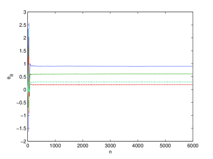
Figure 1: Solid lines: estimates of $\theta_{B}$ by Algorithm V.1. Dotted lines: true values.

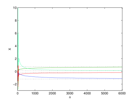
Figure 2: Solid lines: estimates of $X=[\theta_{D}\,\,\,\sigma_{e}^{2}]$ by Algorithm V.1. Dotted lines: true values.

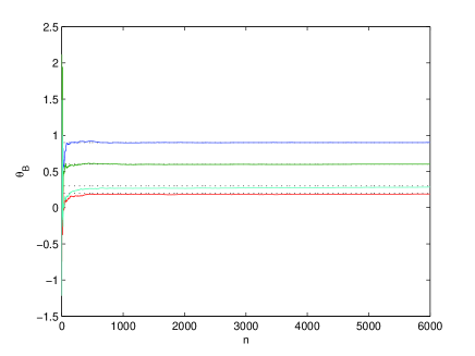
Figure 3: Solid lines: estimates of $\theta_{B}$ by algorithm (33)-(41) with optimal input. Dotted lines: true values.

Figure 4: Solid lines: estimates of $X=[\theta_{D}\,\,\,\sigma_{e}^{2}]$ by algorithm (33)-(41) with optimal input. Dotted lines: true values.

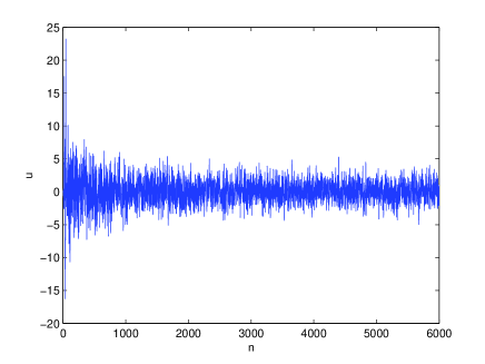
Figure 5: The realization of adaptive input signal $u$ for Algorithm V.1 corresponding to Figs. 4-4.

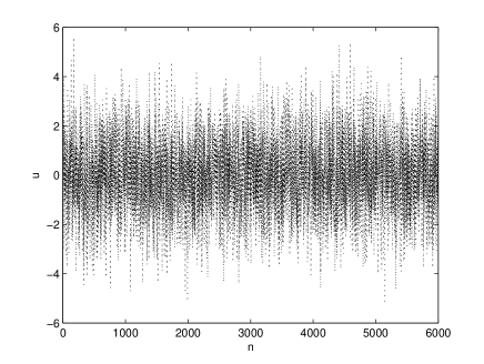
Figure 6: The realization of optimal input signal $u$ corresponding to Figs. 4-4.

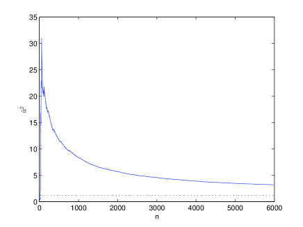
Figure 7: Solid line: the realization of sample input power $\bar{u}^{2}$ for Algorithm V.1 corresponding to Figs. 4, 4 and 8. Dotted line: input power $r_{1}$ of the optimal input.

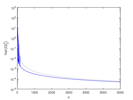
Figure 8: Variance of the estimated ${\mathcal{L}}_{2}$-gain, ${\rm Var}(\|\bar{G}_{N}\|_{2}^{2})$. Solid line: variance estimated from Monte Carlo simulations with the adaptive input. Dotted line: variance estimated from Monte Carlo simulations with the optimal input.

VI-C Simulation results

Generalizing the FIR numerical example in [28], we take the true parameters of the ARARX system with orders $p_{a}=0$, $p_{b}=4$ and $p_{d}=3$ to be ${\theta^{\ast}_{B}}=(0.9\,\,\,0.6\,\,\,0.2\,\,\,0.3)^{T}$, ${\theta^{\ast}_{D}}=(-1.2\,\,\,0.75\,\,\,-0.2)^{T}$ and ${\sigma^{\ast}_{e}}^{2}=0.1$. As in [28], we set the order $m=p_{r}-1=3$ for the linear time-varying system (9). In the following simulations, we employ the algorithm (33)-(41) and choose $D_{\theta}=\{\theta:|\theta_{B}|\leq 3,|\theta_{D}|\leq 10\}$ , $D_{R}$ with $\kappa_{1}=10^{-6}$ and $\kappa_{2}=10^{10}$, initial value $\theta_{0}=[\theta_{B,0}^{T}\,\,\,\theta_{D,0}^{T}]^{T}=0_{7}$ and $R_{0}=I_{7}$.

The total experiment length $N=6\times 10^{3}$, the required accuracy $\gamma=5\times 10^{-5}$ and $\beta_{R}=10^{-2}$. Figs. 4 and 4 show a typical realization of Algorithm V.1 for estimates of $\theta_{B}$ and $X=\begin{bmatrix}\theta_{D}^{T}&\sigma_{e}^{2}\end{bmatrix}^{T}$, respectively, while Figs. 4 and 4 show a typical realization of algorithm (33)-(41) with the optimal input signal that is generated by (9) with parameters obtained by solving the optimization problem (78) with $\theta_{n}={\theta^{\ast}}$. Figs. 8 and 8 shows the input signal $u$ for the same realizations as in Figs. 4-4 and Figs. 4-4, respectively. The realization of the sample input power (63) corresponding to Figs 4-4, as well as $r_{1}$ of the optimal input, are shown in Fig. 8. Fig. 8 shows the variance of the estimated ${\mathcal{L}}_{2}$-gain, ${\rm Var}(\|\bar{G}_{N}\|_{2}^{2})$, estimated from $100$ Monte Carlo simulations with the adaptive input and the optimal input, respectively.

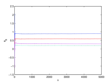
Figure 9: Solid lines: estimates of $\theta_{B}$ by Algorithm V.1. Dotted lines: true values.

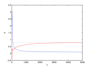
Figure 10: Solid lines: estimates of $X=[\theta_{C}\;\;\sigma_{e}^{2}]$ by Algorithm V.1. Dotted lines: true values.

Figure 11: Solid lines: estimates of $\theta_{B}$ by algorithm (33)-(41) with optimal input. Dotted lines: true values.

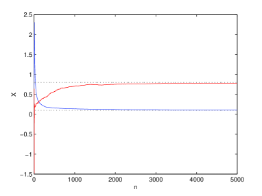
Figure 12: Solid lines: estimate of of $X=[\theta_{C}\;\;\sigma_{e}^{2}]$ by algorithm (33)-(41) with optimal input. Dotted lines: true values.

Figure 13: The realization of adaptive input signal $u$ for Algorithm V.1 corresponding to Figs. 12-12.

Figure 14: The realization of optimal input signal $u$ corresponding to Figs. 12-12.

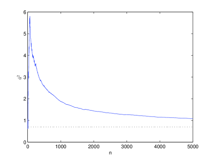
Figure 15: Solid line: the realization of sample input power $\bar{u}^{2}$ for Algorithm V.1 corresponding to Figs. 12, 12 and 16. Dotted line: input power $r_{1}$ of the optimal input.

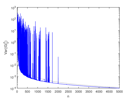
Figure 16: Variance of the estimated ${\mathcal{L}}_{2}$-gain, ${\rm Var}(\|\bar{G}_{N}\|_{2}^{2})$. Solid line: variance estimated from Monte Carlo simulations with the adaptive input. Dotted line: variance estimated from Monte Carlo simulations with the optimal input.

VI-D Simulation results for a MAX system

As noted in Remark II.2, the conditions imposed by Assumption 4 are restrictive. However, we will now illustrate that the proposed algorithm may work even if the conditions in Assumption 4 are not satisfied. To this end, let us generalize the FIR numerical example in [28] to a MAX system. The true parameters of the MAX system with orders $p_{b}=4$ and $p_{c}=1$ are ${\theta^{\ast}_{B}}=\begin{pmatrix}0.9&0.6&0.2&0.3\end{pmatrix}^{T}$, ${\theta^{\ast}_{C}}=c_{1}^{\ast}=0.8$ and ${\sigma^{\ast}_{e}}^{2}=0.1$. In the following simulations, we have used $D_{\theta}=\{\theta:|\theta_{B}|\leq 3,|c_{1}|\leq K_{C}\}$, $D_{R}$ with $\kappa_{1}=10^{-6}$ and $\kappa_{2}=10^{10}$, and initial values $\theta_{0}=[\theta_{B,0}^{T}\,\,\,\theta_{C,0}]^{T}=(0\,\,\,0\,\,\,0\,\,\,0\,\,\,0)^{T}\in D_{0}$ and $R_{0}=I_{5}$. Moreover, $N=5\times 10^{3}$ and $\gamma=10^{-4}$. Note that, as required by Assumption 4, $K_{C}=0.9999<1$ for $D_{C}=\{|\theta_{C}|\leq K_{C}\}$ in [39]. But, from simulations, it appears that $K_{C}$ can be chosen larger. Here we take $K_{C}=5$, which is much larger than what is required by Assumption 4. Notice also that Assumption 6 can not be ensured in this example. Figs. 12 and 12 originate from a typical realization of Algorithm V.1, while Figs. 12 and 12 are typical realizations from the same algorithm, save for that the optimal input is used. The realization of sample input power $\bar{u}^{2}$ corresponding to Figs 12-12, as well as $r_{1}$ of the optimal input, are shown in Fig. 16. Fig. 16 shows the variance of the estimated ${\mathcal{L}}_{2}$-gain, ${\rm Var}(\|\bar{G}_{N}\|_{2}^{2})$, estimated from $100$ Monte Carlo simulations with the adaptive input and the optimal input, respectively. We see that also in this case Algorithm V.1 performs well, despite that some of the assumptions are not satisfied. Thus the algorithm exhibit some degree of robustness.

VII Conclusion

This paper presents sufficient conditions for consistency of an adaptive system consisting of a SISO LTI system, a recursive prediction error estimator and an input generator which uses the parameter estimates. The asymptotic distribution of the resulting parameter estimates has been derived as well.

As an application, we have proposed an adaptive input design method for stable LTI systems based on the certainty equivalence principle. This is a formal development of the scheme outlined in [27], which establishes convergence and asymptotic efficiency. The asymptotic theory is backed-up by a finite-sample simulation study.

Appendix A. Proof of Lemma III.1

Clearly, given any $\theta\in D_{\theta}$, ${\mathbb{E}}[\overline{\varepsilon}_{\theta,n}(\theta)\overline{\varepsilon}_{\theta,n}^{T}(\theta)]\in{\mathbb{R}}^{p_{\theta}\times p_{\theta}}$ is a symmetric positive semidefinite matrix. Furthermore, ${\mathbb{E}}[\overline{\varepsilon}_{\theta,n}(\theta)\overline{\varepsilon}_{\theta,n}^{T}(\theta)]={\mathbb{E}}[\varphi_{n}(\theta)\varphi_{n}^{T}(\theta)]$ is not symmetric positive definite if and only if there exists a nonzero vector $\nu\in{\mathbb{R}}^{p_{\theta}}$ such that $\nu^{T}{\mathbb{E}}[\overline{\varepsilon}_{\theta,n}(\theta)\overline{\varepsilon}_{\theta,n}^{T}(\theta)]\nu={\mathbb{E}}[\nu^{T}\overline{\varepsilon}_{\theta,n}(\theta)\overline{\varepsilon}_{\theta,n}^{T}(\theta)\nu]={\mathbb{E}}[|\nu^{T}\overline{\varepsilon}_{\theta,n}(\theta)|^{2}]={\mathbb{E}}[|\nu^{T}\varphi_{n}(\theta)|^{2}]=0$.

Let

$$\bar{G}^{\ast}(q)=\frac{B^{\ast}(q)}{A^{\ast}(q)F^{\ast}(q)}\quad{\rm and}\quad\bar{H}^{\ast}(q)=\frac{C^{\ast}(q)}{A^{\ast}(q)D^{\ast}(q)},$$

then $y_{n}(\theta)=\bar{G}^{\ast}(q)u_{n}+\bar{H}^{\ast}(q)e_{n}$. By (25), we observe that

$$\overline{\varepsilon}_{\theta,n}(\theta)=\overline{\varepsilon}_{\theta,n}(\theta)=\begin{bmatrix}F_{u}(q,\theta)&F_{e}(q,\theta)\end{bmatrix}\begin{bmatrix}u_{n}&e_{n}\end{bmatrix}^{T}=F_{u}(q,\theta)u_{n}+F_{e}(q,\theta)e_{n}$$ (79)

and hence ${\mathbb{E}}[\overline{\varepsilon}_{\theta,n}(\theta)\overline{\varepsilon}_{\theta,n}^{T}(\theta)]$ are continuous on $D_{\theta}$ since both $F_{u}(q,\theta)$ and $F_{e}(q,\theta)$ are continuous on $D_{\theta}$, where

$$F_{u}(q,\theta)=\begin{bmatrix}F_{u\widetilde{y}}(q)&-F_{u\widetilde{u}}(q)&F_{u\widetilde{w}}(q,\theta)&-F_{u\tilde{\varepsilon}}(q,\theta)&F_{u\widetilde{v}}(q,\theta)\end{bmatrix}^{T},$$

$$F_{e}(q,\theta)=\begin{bmatrix}F_{e\widetilde{y}}(q)&0_{p_{b}}^{T}&0_{p_{f}}^{T}&-F_{e\tilde{\varepsilon}}(q,\theta)&F_{e\widetilde{v}}(q,\theta)\end{bmatrix}^{T},$$

$$F_{u\widetilde{y}}(q)=\left[q^{-1}\;\;\;\cdots\;\;\;q^{-p_{a}}\right]\bar{G}^{\ast}(q),\quad F_{u\widetilde{u}}(q)=\left[q^{-1}\;\;\;\cdots\;\;\;q^{-p_{b}}\right],$$

$$F_{u\widetilde{w}}(q,\theta)=\left[q^{-1}\;\;\;\cdots\;\;\;q^{-p_{f}}\right]F_{wu}(q,\theta),\;\;F_{wu}(q,\theta)=\frac{B(q,\theta_{B})}{F(q,\theta_{F})},$$

$$F_{u\tilde{\varepsilon}}(q,\theta)=\left[q^{-1}\;\;\;\cdots\;\;\;q^{-p_{c}}\right]F_{\varepsilon u}(q,\theta),\;\;F_{\varepsilon u}(q,\theta)=\frac{D(q,\theta_{D})}{C(q,\theta_{C})}F_{vu}(q,\theta),$$

$$F_{u\widetilde{v}}(q,\theta)=\left[q^{-1}\;\;\;\cdots\;\;\;q^{-p_{d}}\right]F_{vu}(q,\theta),\;\;F_{vu}(q,\theta)=A(q,\theta_{A})\bar{G}^{\ast}(q)-F_{wu}(q,\theta),$$

$$F_{e\widetilde{y}}(q)=\left[q^{-1}\;\;\;\cdots\;\;\;q^{-p_{a}}\right]\bar{H}^{\ast}(q),$$

$$F_{e\tilde{\varepsilon}}(q,\theta)=\left[q^{-1}\;\;\;\cdots\;\;\;q^{-p_{c}}\right]F_{\varepsilon e}(q,\theta),\;\;F_{\varepsilon e}(q,\theta)=\frac{D(q,\theta_{D})A(q,\theta_{A})}{C(q,\theta_{C})}\bar{H}^{\ast}(q),$$

$$F_{e\widetilde{v}}(q,\theta)=\left[q^{-1}\;\;\;\cdots\;\;\;q^{-p_{d}}\right]F_{ve}(q,\theta),\;\;F_{ve}(q,\theta)=A(q,\theta_{A})\bar{H}^{\ast}(q).$$

Particularly, we have

$$\overline{\varepsilon}_{\theta,n}({\theta^{\ast}})=F_{u}(q,{\theta^{\ast}})u_{n}+F_{e}(q,{\theta^{\ast}})e_{n},$$ (80)

where $F_{u}(q,{\theta^{\ast}})=\begin{bmatrix}F_{u\widetilde{y}}(q)&-F_{u\widetilde{u}}(q)&F_{u\widetilde{w}}(q,{\theta^{\ast}})&0_{p_{c}}^{T}&0_{p_{d}}^{T}\end{bmatrix}^{T}$ and
$F_{e}(q,{\theta^{\ast}})=\begin{bmatrix}F_{e\widetilde{y}}(q)&0_{p_{b}}^{T}&0_{p_{f}}^{T}&-F_{e\tilde{\varepsilon}}(q,{\theta^{\ast}})&F_{e\widetilde{v}}(q,{\theta^{\ast}})\end{bmatrix}^{T}$.

Note that $\{u_{n}\}$ is generated by (9) with $\{s_{n}\}$ independent of $\{e_{n}\}$. For any nonzero vector $\nu\in{\mathbb{R}}^{p_{\theta}}$, we have

$$\nu^{T}\overline{\varepsilon}_{{\theta^{\ast}},n}(\theta)=\nu^{T}F_{u}(q,{\theta^{\ast}})u_{n}+\nu^{T}F_{e}(q,{\theta^{\ast}})e_{n},$$ (81)

and, by Parseval’s formula,

$${\mathbb{E}}[|\nu^{T}\overline{\varepsilon}_{\theta,n}({\theta^{\ast}})|^{2}]=\frac{1}{2\pi}\int_{-\pi}^{\pi}\begin{bmatrix}\nu^{T}F_{u}(e^{i\omega},{\theta^{\ast}})&\nu^{T}F_{e}(e^{i\omega},{\theta^{\ast}})\end{bmatrix}\begin{bmatrix}\Psi_{u}(e^{i\omega})&0\\ 0&{\sigma^{\ast}_{e}}^{2}\end{bmatrix}\begin{bmatrix}F_{u}^{T}(e^{i\omega},{\theta^{\ast}})\nu\\ F_{e}^{T}(e^{i\omega},{\theta^{\ast}})\nu\end{bmatrix}{\mathrm{d}}\omega.$$ (82)

Since Assumption 3 implies that there does not exist a vector $\nu\neq 0_{p_{\theta}}$ such that

$$\nu^{T}F_{u}(e^{i\omega},{\theta^{\ast}})=\nu^{T}F_{e}(e^{i\omega},{\theta^{\ast}})=0$$

for almost all $\omega$, (82) with (29) yields ${\mathbb{E}}[|\nu^{T}\overline{\varepsilon}_{{\theta^{\ast}},n}({\theta^{\ast}})|^{2}]>0$ for any nonzero vector $\nu\in{\mathbb{R}}^{p_{\theta}}$, or say, ${\mathbb{E}}[\overline{\varepsilon}_{\theta,n}({\theta^{\ast}})\overline{\varepsilon}_{\theta,n}^{T}({\theta^{\ast}})]>0$. Since Assumption 3 holds on some neighborhood of ${\theta^{\ast}}$ (see Remark II.4), it follows the desired result.

Appendix B. Notations in adaptive system (33)-(41)

$\Phi_{n}=[\Phi_{1,n}^{T}\,\,\,\Phi_{2,n}^{T}\,\,\,\Phi_{3,n}^{T}\,\,\,\Phi_{4,n}^{T}\,\,\,\Phi_{5,n}^{T}\,\,\,\Phi_{6,n}^{T}\,\,\,\Phi_{7,n}^{T}\,\,\,\Phi_{8,n}^{T}]^{T}\in{\mathbb{R}}^{m+p_{\theta}+n_{\xi}+2}$, $\Phi_{1,n}=z_{n}$, $\Phi_{2,n}=\widetilde{u}_{n-1}$, $\Phi_{3,n}=e_{n}$, $\Phi_{4,n}=\xi_{n}$, $\Phi_{5,n}=\widetilde{y}_{n-1}$, $\Phi_{6,n}=\widetilde{w}_{n-1}$, $\Phi_{7,n}=\widetilde{v}_{n-1}$, $\Phi_{8,n}=\tilde{\varepsilon}_{n-1}$, $\eta_{n}=[e_{n+1}\,\,\,s_{n}]^{T}$,

$$A_{\Phi}(\theta)=\begin{bmatrix}A_{z}(r(\theta))&0&0&0&0&0&0&0\\ A_{21}&A_{22}&0&0&0&0&0&0\\ 0&0&0&0&0&0&0&0\\ B_{\xi}C_{z}(r(\theta))&0&K_{\xi}&A_{\xi}&0&0&0&0\\ 0&0&A_{53}&A_{54}&A_{55}&0&0&0\\ 0&A_{62}&0&0&0&\widetilde{F}&0&0\\ 0&A_{72}&A_{73}&A_{74}&A_{75}&A_{76}&A_{77}&0\\ 0&A_{82}&A_{83}&A_{84}&A_{85}&A_{86}&A_{87}&\widetilde{C}\end{bmatrix},\;\;\;B_{\Phi}(\theta)=\begin{bmatrix}0&B_{z}(r(\theta))\\ 0&B_{22}\\ 1&0\\ 0&B_{\xi}D_{z}(r(\theta))\\ 0&0\\ 0&0\\ 0&0\\ 0&0\end{bmatrix},$$

$$Q(\theta,\Phi_{n+1})=-R_{n}^{-1}(\theta)\varepsilon_{\theta,n+1}(\theta)\left(C_{\xi}\Phi_{4,n+1}+\Phi_{3,n+1}+\theta^{T}\varepsilon_{\theta,n+1}\right),$$

$$R_{n+1}(\theta)=\frac{n}{n+1}R_{n}(\theta)+\frac{1}{n+1}\varepsilon_{\theta,n+1}\varepsilon_{\theta,n+1}^{T}$$

$\varepsilon_{\theta,n}(\theta)=\begin{bmatrix}\Phi_{5,n}\\ -\Phi_{2,n}\\ \Phi_{6,n}\\ -\Phi_{8,n}\\ \Phi_{7,n}\end{bmatrix}\in{\mathbb{R}}^{p_{\theta}}$, $A_{21}=\begin{bmatrix}C_{z}(r(\theta))\\ 0\\ \vdots\\ 0\end{bmatrix}\in{\mathbb{R}}^{p_{b}\times m}$, $A_{22}=\widetilde{I}_{u}=\begin{bmatrix}0&0\\ I_{p_{b}-1}&0\end{bmatrix}\in{\mathbb{R}}^{p_{b}\times p_{b}}$, $B_{22}=\begin{bmatrix}D_{z}(r(\theta))\\ 0\\ \vdots\\ 0\end{bmatrix}\in{\mathbb{R}}^{p_{b}}$, $A_{53}=\widetilde{I}^{e}_{y}=\begin{bmatrix}1\\ 0\\ \vdots\\ 0\end{bmatrix}\in{\mathbb{R}}^{p_{a}}$, $A_{54}=\begin{bmatrix}C_{\xi}\\ 0\\ \vdots\\ 0\end{bmatrix}\in{\mathbb{R}}^{p_{a}\times n_{\xi}}$, $A_{55}=\widetilde{I}_{y}=\begin{bmatrix}0&0\\ I_{p_{a}-1}&0\end{bmatrix}\in{\mathbb{R}}^{p_{a}\times p_{a}}$, $A_{62}=\begin{bmatrix}\theta_{B}^{T}\\ 0\\ \vdots\\ 0\end{bmatrix}\in{\mathbb{R}}^{p_{f}\times p_{b}}$, $A_{72}=\begin{bmatrix}-\theta_{B}^{T}\\ 0\\ \vdots\\ 0\end{bmatrix}\in{\mathbb{R}}^{p_{d}\times p_{b}}$, $A_{73}=\begin{bmatrix}1\\ 0\\ \vdots\\ 0\end{bmatrix}\in{\mathbb{R}}^{p_{d}}$, $A_{74}=\begin{bmatrix}C_{\xi}\\ 0\\ \vdots\\ 0\end{bmatrix}\in{\mathbb{R}}^{p_{d}\times n_{\xi}}$, $A_{75}=\begin{bmatrix}\theta_{A}^{T}\\ 0\\ \vdots\\ 0\end{bmatrix}\in{\mathbb{R}}^{p_{d}\times p_{a}}$, $A_{76}=\begin{bmatrix}\theta_{F}^{T}\\ 0\\ \vdots\\ 0\end{bmatrix}\in{\mathbb{R}}^{p_{d}\times p_{f}}$, $A_{77}=\widetilde{I}_{v}=\begin{bmatrix}0&0\\ I_{p_{d}-1}&0\end{bmatrix}\in{\mathbb{R}}^{p_{d}\times p_{d}}$, $A_{82}=\begin{bmatrix}-\theta_{B}^{T}\\ 0\\ \vdots\\ 0\end{bmatrix}\in{\mathbb{R}}^{p_{c}\times p_{b}}$, $A_{83}=\begin{bmatrix}1\\ 0\\ \vdots\\ 0\end{bmatrix}\in{\mathbb{R}}^{p_{c}}$, $A_{84}=\begin{bmatrix}C_{\xi}\\ 0\\ \vdots\\ 0\end{bmatrix}\in{\mathbb{R}}^{p_{c}\times n_{\xi}}$, $A_{86}=\begin{bmatrix}\theta_{A}^{T}\\ 0\\ \vdots\\ 0\end{bmatrix}\in{\mathbb{R}}^{p_{c}\times p_{a}}$, $A_{86}=\begin{bmatrix}-\theta_{F}^{T}\\ 0\\ \vdots\\ 0\end{bmatrix}\in{\mathbb{R}}^{p_{c}\times p_{f}}$ and $A_{87}=\begin{bmatrix}\theta_{D}^{T}\\ 0\\ \vdots\\ 0\end{bmatrix}\in{\mathbb{R}}^{p_{c}\times p_{d}}$.

Appendix C. Some useful results in literature

Definition C.1: A random process $\{\bar{s}_{n}\}_{n\geq 0}$ is $L$-mixing with respect to the $\sigma$-algebras $({\mathcal{F}}_{n},{\mathcal{F}}_{n}^{+})$, $n\geq 0$, if the following conditions are satisfied:

• $\bar{s}_{n}$ is ${\mathcal{F}}_{n}$ measurable,

• $\bar{s}_{n}=O_{M}(1)$,

• $\sum_{t=0}^{\infty}\gamma_{k}(t)<\infty$ for all $1\leq k<\infty$, where

  $$\gamma_{k}(t)=\sup_{n\geq t}{\mathbb{E}}^{1/k}\left[\big{|}\bar{s}_{n}-{\mathbb{E}}[\bar{s}_{n}|{\mathcal{F}}_{n}^{+}]\big{|}^{k}\right],\,\,\,t\geq 0.$$

Some useful theorems derived from the main results in [25, 26] are given as follows, which are applied to develop our results in this paper.

Condition C.1: The noise $\{\eta_{n}\}$ in the system (36) is a sequence of independent random variables such that

$$\sup_{n}{\mathbb{E}}[\exp{(\alpha_{\eta}|\eta_{n}|^{2})}]<\infty$$ (83)

holds for some $\alpha_{\eta}>0$.

Condition C.2: The time-varying system (36) is bounded input-bounded output (BIBO) stable.

Condition C.3 The families of matrices $A_{\Phi}(\theta)$ and $B_{\Phi}(\theta)$, $\theta\in D_{\theta}$, are triply continuously differentiable with bounded partial derivatives up to second order in $D_{\theta}$.

Condition C.4: Denote by $X(t;\bar{t},\bar{X})$ the solution to ODE (42) for $t\geq\bar{t}\geq 0$ with $X_{\bar{t}}=\bar{X}$. Assume that (42) has a unique equilibrium point $X_{\ast}\in{\rm int}D_{X00}$ on $D_{X}$ and $\bar{X}\in{\rm int}D_{X00}$, where $D_{X00}\subset{\rm int}D_{X}$ is a compact convex set that is invariant for (42) and $\{X(t;\bar{t},\bar{X}):t>\bar{t}\geq 0,\bar{X}\in D_{X00}\}\subset{\rm int}D_{X00}$. Moreover, for every $\bar{X}\in D_{X00}$, we have the Lyapunov exponent $-\alpha<-1/2$, i.e., there is a constant $\bar{C}_{0}>0$ such that

$$\left|\frac{\partial}{\partial\bar{X}}X(t;\bar{t},\bar{X})\right|\leq\bar{C}_{0}\exp{(-\alpha(t-\bar{t}\,))}$$ (84)

for all $t>\bar{t}\geq 0$.

A variant of [25, Theorem 4.1] (see also [26, Theorem 3.3]) is given as follows

Theorem C.1: Assume that Conditions C.1, C.2, C.3 hold, and that Condition C.4 also holds with $\bar{X}=X_{0}=(\theta_{0},R_{0})\in{\rm int}D_{X00}$. Then $\{X_{n}\}$ with $X_{n}=(\theta_{n},R_{n})$ computed by the recursive stochastic algorithm (33)-(41) satisfies

$$X_{n}-X_{\ast}=O_{M}(n^{-1/2}).$$ (85)

In particular $X_{n}\rightarrow X_{\ast}$ almost surely as $n\rightarrow\infty$.

Appendix D. Proof of Theorem IV.1

It is observed that, by (4) and (10), Condition C.1 is satisfied. Let us consider Condition C.2, i.e., the BIBO stability of the linear time-varying system (36). According to Lemma 27.4 in [70], the time-varying system (36) is BIBO stable if the set $\{B_{\Phi}(\theta)):\theta\in D_{\theta}\}$ is bounded and the automous system obtained with $B_{\Phi}(\theta)=0$ is uniformly exponentially stable.

From Appendix B we have that $B_{\Phi}(\theta)$ depends only on $\theta$ through $B_{z}(r(\theta))$ and $D_{z}(r(\theta))$, which by assumption are bounded.

Uniform exponential stability is equivalent to uniform asymptotic stability (see, e.g., [6]), which in turn is equivalent to that the joint spectral radius of the set of state transition matrices $\Sigma_{\Phi}=\{A_{\Phi}(\theta):\theta\in D_{\theta}\}$ is less than one, when this set is bounded [41, Corollary 1.1, p.21] (see also [9]). Below we will show that $\rho(\Sigma_{\Phi})<1$ but first we need to establish that $\Sigma_{\Phi}$ is bounded. From Appendix B we have that $A_{\Phi}(\theta)$ depends affinely on $A_{z}(r(\theta))$, $C_{z}(r(\theta))$, and $\theta$. There are no other $\theta$-dependencies in $A_{\Phi}(\theta)$. By Assumption 5 $A_{z}(r(\theta))$, $C_{z}(r(\theta))$ are bounded on $D_{\theta}$. Furthermore, $D_{\theta}$ is compact due to Assumption 4, and hence $\theta\in D_{\theta}$ is bounded. Hence $\Sigma_{\Phi}$ is bounded. We will now analyze the joint spectral radius of $\Sigma_{\Phi}$.

Let $\Sigma_{\Phi}^{n}=\{A_{n}\cdots A_{2}A_{1}:A_{k}\in\Sigma_{\Phi},k=1,2,\cdots,n\}$. It is easy to observe that every product $\bar{A}_{\Phi,n}\in\Sigma_{\Phi}^{n}$ is a lower triangular matrix of the form

$$\bar{A}_{\Phi,n}=\begin{bmatrix}\bar{A}_{z,n}&0&0&0&0&0&0&0\\ \ast&(\widetilde{I}_{u})^{n}&0&0&0&0&0&0\\ 0&0&0&0&0&0&0&0\\ \ast&\ast&\ast&(A_{\xi})^{n}&0&0&0&0\\ \ast&\ast&\ast&\ast&(\widetilde{I}_{y})^{n}&0&0&0\\ \ast&\ast&\ast&\ast&\ast&\bar{F}_{n}&0&0\\ \ast&\ast&\ast&\ast&\ast&\ast&(\widetilde{I}_{v})^{n}&0\\ \ast&\ast&\ast&\ast&\ast&\ast&\ast&\bar{C}_{n}\end{bmatrix}$$ (86)

for all $n\geq 1$, where $\bar{A}_{z,n}\in\Sigma_{z}^{n}$, $\bar{C}_{n}\in\Sigma_{C}^{n}$, $\bar{F}_{n}\in\Sigma_{F}^{n}$ and the entries denoted by $\ast$ can be zero or nonzero. Thus the eigenvalues of $\bar{A}_{\Phi,n}$ are given by the eigenvalues of the matrices on the block-diagonal. Obviously, $(\widetilde{I}_{u})^{n}$, $(\widetilde{I}_{y})^{n}$ and $(\widetilde{I}_{v})^{n}$ are strictly lower triangular matrices (i.e., lower triangular matrices having zeros along their main diagonals) for all $n\geq 1$. In fact, there is a positive integer $n_{0}$ such that $(\widetilde{I}_{u})^{n}=0$, $(\widetilde{I}_{y})^{n}=0$ and $(\widetilde{I}_{v})^{n}=0$ for all $n\geq n_{0}$ since all $\widetilde{I}_{u}$, $\widetilde{I}_{y}$ and $\widetilde{I}_{v}$ are nilpotent matrices. Thus these matrices have all eigenvalues at the origin. Next, note that the transition matrix $A_{\xi}$ has all its eigenvalues strictly inside the unit circle, that is $\rho(A_{\xi})<1$. Recalling (6), the above gives

$$\rho_{n}(\Sigma_{\Phi})=\max\left\{\rho_{n}(\Sigma_{z}),\rho(A_{\xi}),\rho_{n}(\Sigma_{C}),\rho_{n}(\Sigma_{F})\right\}$$ (87)

for all $n\geq 1$. But this combined with Assumptions 4 and 5 and that $\rho(A_{\xi})<1$, immediately implies

$$\rho(\Sigma_{\Phi})=\limsup_{n\to\infty}\rho_{n}(\Sigma_{\Phi})<1.$$ (88)

Thus, as argued above, Lemma 27.4 in [70] and [41, Corollary 1.1, p21] (see also [9]) imply that the switching system (36) is (uniformly asymptotically) stable and therefore BIBO stable. Therefore, Condition C.2 is satisfied.

Let us proceed to show the asymptotic stability of the associated ODE (42). Since $G(\theta)$ is continuous on the compact $D_{\theta}$ (see Appendix A), there exists $\kappa_{0}>0$ such that $0\leq G(\theta)<\kappa_{0}I_{p_{\theta}}$ for all $\theta\in D_{\theta}$. Note that ODE (42b) with initial value $R_{0}>0$ gives

$$R_{t}=e^{-\frac{1}{2}I_{p_{\theta}}t}R_{0}e^{-\frac{1}{2}I_{p_{\theta}}t}+e^{-\frac{1}{2}I_{p_{\theta}}t}\left[\int_{0}^{t}e^{\frac{1}{2}I_{p_{\theta}}\tau}G(\theta_{\tau})e^{\frac{1}{2}I_{p_{\theta}}\tau}{\mathrm{d}}\tau\right]e^{-\frac{1}{2}I_{p_{\theta}}t}$$ (89)

for all $t\geq 0$, which yields

$$\kappa_{r}e^{-t}I_{p_{\theta}}<e^{-\frac{1}{2}I_{p_{\theta}}t}R_{0}e^{-\frac{1}{2}I_{p_{\theta}}t}\leq R_{t}\leq R_{0}+e^{-\frac{1}{2}I_{p_{\theta}}t}\left[\int_{0}^{t}e^{\frac{1}{2}I_{p_{\theta}}\tau}\kappa_{0}I_{p_{\theta}}e^{\frac{1}{2}I_{p_{\theta}}\tau}{\mathrm{d}}\tau\right]e^{-\frac{1}{2}I_{p_{\theta}}t}$$

$$=R_{0}+\kappa_{0}(1-e^{-t})I_{p_{\theta}}<\kappa_{2}I_{p_{\theta}}\qquad\qquad\qquad\quad$$ (90)

for all $t\in[0,\infty)$, where $\kappa_{2}=\kappa_{R}+\kappa_{0}$ with $\kappa_{R}I_{p_{\theta}}>R_{0}>\kappa_{r}I_{p_{\theta}}>0$. This implies that

$$\kappa_{2}^{-1}I_{p_{\theta}}<R_{t}^{-1}<\kappa_{r}^{-1}e^{t}I_{p_{\theta}},\qquad\forall\;t\in[0,\infty).$$ (91)

Recall that the asymptotic cost function $W(\theta)$ defined by (18) has exactly one minimum ${\theta^{\ast}}$ on $D_{\theta}$ since (27) has the unique solution $\theta={\theta^{\ast}}$. Obviously, $W(\theta)\geq W({\theta^{\ast}})>0$ for all $\theta\in D_{\theta}$. By (42a) and Assumption 7, we observe

$$\frac{{\mathrm{d}}}{{\mathrm{d}}t}W(\theta)=-W_{\theta}^{T}(\theta)R_{t}^{-1}W_{\theta}(\theta)\leq-\lambda_{m}(R_{t}^{-1})\big{|}W_{\theta}(\theta)\big{|}^{2}<-\kappa_{2}^{-1}\big{|}W_{\theta}(\theta)\big{|}^{2}$$ (92)

for all $t\in[0,\infty)$, and, particularly,

$$\frac{{\mathrm{d}}}{{\mathrm{d}}t}W(\theta)\leq-\kappa_{2}^{-1}w_{\theta^{\ast}}^{2}<0$$

for all $\theta\in D_{\theta}\backslash D_{\theta^{\ast}}$, where $w_{\theta^{\ast}}^{2}=\inf_{\theta\in D_{\theta}\backslash D_{\theta^{\ast}}}\big{|}W_{\theta}(\theta)\big{|}^{2}$. This implies that there is a finite positive constant $t_{{\theta^{\ast}}}\leq W(\theta_{0})/(\kappa_{2}^{-1}w_{\theta^{\ast}}^{2})$ such that $\theta_{t}\in D_{{\theta^{\ast}}}$ for all $t\geq t_{{\theta^{\ast}}}$. By Lemma III.1, there is a positive constant $\kappa_{\theta^{\ast}}$ such that $G(\theta)\geq\kappa_{\theta^{\ast}}I_{p_{\theta}}$ for all $\theta\in D_{\theta^{\ast}}$. This combined with (89) and (Appendix D. Proof of Theorem IV.1) gives

$$R_{t}\geq R_{t_{\theta^{\ast}}}+e^{-\frac{1}{2}I_{p_{\theta}}t}\left[\int_{t_{\theta^{\ast}}}^{t}e^{\frac{1}{2}I_{p_{\theta}}\tau}\kappa_{\theta^{\ast}}I_{p_{\theta}}e^{\frac{1}{2}I_{p_{\theta}}\tau}{\mathrm{d}}\tau\right]e^{-\frac{1}{2}I_{p_{\theta}}t}>\kappa_{r}e^{-t_{\theta^{\ast}}}I_{p_{\theta}}+\kappa_{\theta^{\ast}}e^{-t_{\theta^{\ast}}}I_{p_{\theta}}$$ (93)

for all $t\geq t_{\theta^{\ast}}$. But (Appendix D. Proof of Theorem IV.1) and (93) immediately yield $R_{t}>\kappa_{1}I_{p_{\theta}}$ for all $t\geq 0$, where $\kappa_{1}=\kappa_{r}e^{-t_{\theta^{\ast}}}>0$. This combined with (Appendix D. Proof of Theorem IV.1) and (91) gives

$$\kappa_{1}I_{p_{\theta}}<R_{t}<\kappa_{2}I_{p_{\theta}}\;\;\;{\rm and}\;\;\;\kappa_{2}^{-1}I_{p_{\theta}}<R_{t}^{-1}<\kappa_{1}^{-1}I_{p_{\theta}}$$ (94)

for all $t\geq 0$, where positive constants $\kappa_{1}$ and $\kappa_{2}$ can be used to define $D_{R}$ in (34). So (92) holds for all $t\geq 0$. But, according to [50, VIII. Theorem, p66], this implies that the equilibrium ${\theta^{\ast}}$ of (42a) is asymptotically stable, which also yields $R_{t}\to R^{\ast}=G({\theta^{\ast}})$ as $t\to\infty$. Therefore, the equilibrium $({\theta^{\ast}},R^{\ast})$ of ODE (42) is asymptotically stable.

Finally, we show (45) as follows. Note that Assumption 8 implies Condition C.3 and the Jacobian matrix of (42) at $({\theta^{\ast}},R^{\ast})$ has the structure

$$\begin{pmatrix}-I_{p_{\theta}}&0\\ \ast&-I_{p_{\theta}}\end{pmatrix},$$ (95)

all eigenvalues of which are equal to $-1$. It follows that Condition C.4 is satisfied with the Lyapunov exponent $-\alpha=-1+c$ for any $c>0$ in some invariant neighborhood of $({\theta^{\ast}},R^{\ast})$ (see also proof of [25, Theorem 4.2]). Let $D_{\theta,R}$ be a compact convex invariant neighborhood such that $({\theta^{\ast}},R^{\ast})\in{\rm int}D_{\theta,R}$ and Condition C.4 is satisfied with the Lyapunov exponent $-\alpha<-1/2$. The proof of [37, Theorem 3.1] shows that there exists a sample dependent finite number $N_{\theta,R}$ such that $\{(\theta_{n},R_{n})\}_{n\geq N_{\theta,R}}\subset{\rm int}D_{\theta,R}$ almost surely. Let us consider the sequence $\{(\theta_{n},R_{n})\}_{n\geq N_{\theta,R}}$. But, by Theorem C.1, $\{(\theta_{n},R_{n})\}_{n\geq N_{\theta,R}}$ satisfies

$$\theta_{n}-{\theta^{\ast}}=O_{M}((n-N_{\theta,R})^{-1/2})\quad{\rm and}\quad R_{n}-R^{\ast}=O_{M}((n-N_{\theta,R})^{-1/2})$$ (96)

a.s. as $n\to\infty$. It is noticed that

$$n^{1/2}=O_{M}((n-N_{\theta,R})^{1/2})$$ (97)

a.s. as $n\to\infty$ since ${\mathbb{P}}\{N_{\theta,R}<\infty\}=1$. So, by Cauchy-Schwarz inequality, (96) and (97) imply (45). Almost sure convergence follows from (45) as noted after Theorem 4.1 in [25]. This completes the proof.

Appendix E. Proof of Theorem IV.2

Since, according to the proof of Theorem IV.1 (see Appendix D), the switching system (36) is BIBO stable and hence is uniformly exponentially stable, there are $C_{\Phi}>0$ and $\lambda_{\Phi}\in(0,1)$ such that (see [61])

$$|\Phi_{n}|\leq C_{\Phi}\lambda_{\Phi}^{n}|\Phi_{0}|+\sum_{k=1}^{n}C_{\Phi}\lambda_{\Phi}^{k}|\eta_{n-k}|=:\widehat{\Phi}_{n}.$$ (98)

Therefore, $\{\widehat{\Phi}_{n}\}$ and hence $\{\Phi_{n}\}$ are $L$-mixing processes since $\{e_{n}\}$, $\{w_{n}\}$ and hence $\{\eta_{n}\}$ are $L$-mixing processes (see [24]). It follows that the process

$$\Delta\Phi_{n}=\Phi_{n}-\Phi^{\ast}_{n}$$ (99)

is $L$-mixing, where $\{\Phi^{\ast}_{n}\}$ is generated by (36) with $\theta_{n}={\theta^{\ast}}$ and $\varepsilon_{\theta,n}^{\ast}=\varepsilon_{\theta,n}({\theta^{\ast}})=-\varphi_{n}({\theta^{\ast}})=\begin{bmatrix}\widetilde{y}_{n-1}^{T}({\theta^{\ast}})&-\widetilde{u}_{n-1}^{T}({\theta^{\ast}})&\widetilde{w}_{n-1}^{T}({\theta^{\ast}})&-\tilde{\varepsilon}_{n-1}^{T}({\theta^{\ast}})&\widetilde{v}_{n-1}^{T}({\theta^{\ast}})\end{bmatrix}^{T}$. Moreover, since system (36) is uniformly exponentially stable and, by Theorem IV.1, $\theta_{n}\to{\theta^{\ast}}$ a.s. as $n\to\infty$, and using Assumption 8 we have $\Delta\Phi_{n}\to 0$ a.s. as $n\to\infty$. Then the stability of $A_{\Phi}(\cdot)$ and the boundedness of $B_{\Phi}(\cdot)$ imply that $\Delta\Phi_{n}=o_{M}(1)$, i.e., $\Delta\Phi_{n}\to 0$ in ${\mathcal{L}}_{q}$-norm for all $q\geq 1$. Clearly, this yields that

$$\Delta\varepsilon_{\theta,n}=\varepsilon_{\theta,n}-\varepsilon_{\theta,n}^{\ast}$$ (100)

is an $L$-mixing process and $\Delta\varepsilon_{\theta,n}=o_{M}(1)$ since

$$\Delta\varepsilon_{\theta,n}=[\Delta\Phi_{5,n}^{T}\,\,\,-\Delta\Phi_{2,n}^{T}\,\,\,\Delta\Phi_{6,n}^{T}\,\,\,-\Delta\Phi_{8,n}^{T}\,\,\,\Delta\Phi_{7,n}^{T}]^{T},$$

where $\Delta\Phi_{k,n}=\Phi_{k,n}-\Phi^{\ast}_{k,n}$ for $k=1,2,\cdots,8$.

Note that $\{\varepsilon_{\theta,n}^{\ast}\}$ is an $L$-mixing process and therefore

$$\frac{1}{n}\sum_{k=1}^{n}\varepsilon_{\theta,k}^{\ast}(\varepsilon_{\theta,k}^{\ast})^{T}\to R^{\ast}\quad\text{a.s.}$$ (101)

and hence in law as $n\to\infty$. Moreover, by Cauchy-Schwarz inequality, we observe

$$\frac{1}{n}\sum_{k=1}^{n}\big{[}\varepsilon_{\theta,k}^{\ast}\Delta\varepsilon_{\theta,k}^{T}+\Delta\varepsilon_{\theta,k}(\varepsilon_{\theta,k}^{\ast})^{T}+\Delta\varepsilon_{\theta,k}\Delta\varepsilon_{\theta,k}^{T}\big{]}\to 0,$$ (105)

$$\frac{1}{n}\sum_{k=1}^{n}\varepsilon_{\theta,k}\Delta\widetilde{w}_{k-1}^{T}=\frac{1}{n}\sum_{k=1}^{n}\big{(}\varepsilon_{\theta,k}^{\ast}+\Delta\varepsilon_{\theta,k}\big{)}\Delta\widetilde{w}_{k-1}^{T}\to 0,$$

$$\frac{1}{n}\sum_{k=1}^{n}\varepsilon_{\theta,k}\Delta\tilde{\varepsilon}_{k-1}^{T}=\frac{1}{n}\sum_{k=1}^{n}\big{(}\varepsilon_{\theta,k}^{\ast}+\Delta\varepsilon_{\theta,k}\big{)}\Delta\tilde{\varepsilon}_{k-1}^{T}\to 0,$$

$$\frac{1}{n}\sum_{k=1}^{n}\varepsilon_{\theta,k}\Delta\widetilde{v}_{k-1}^{T}=\frac{1}{n}\sum_{k=1}^{n}\big{(}\varepsilon_{\theta,k}^{\ast}+\Delta\varepsilon_{\theta,k}\big{)}\Delta\widetilde{v}_{k-1}^{T}\to 0$$

in ${\mathcal{L}}_{q}$ for any $q\geq 1$ and hence in law as $n\to\infty$. But, since both $\{\varepsilon_{\theta,n}\}$ and $\{\varepsilon_{\theta,n}^{\ast}\}$ are $L$-mixing processes, (101) and (105) give

$$\frac{1}{n}\sum_{k=1}^{n}\varepsilon_{\theta,k}\varepsilon_{\theta,k}^{T}\to R^{\ast}$$ (106)

in ${\mathcal{L}}_{q}$ for any $q\geq 1$ and hence in law as $n\to\infty$. And the combination of (11), (27) and (105)-(105) yields

$$\left(\frac{1}{n}\sum_{k=1}^{n}\varepsilon_{\theta,k}\varepsilon_{\theta,k}^{T}\right)(\theta_{n}-{\theta^{\ast}})$$ (107)

$${}=\frac{1}{n}\sum_{k=1}^{n}\varepsilon_{\theta,k}(-\Delta\widetilde{w}_{k-1}^{T}{\theta^{\ast}_{F}}+\Delta\tilde{\varepsilon}_{k-1}^{T}{\theta^{\ast}_{C}}-\Delta\widetilde{v}_{k-1}^{T}{\theta^{\ast}_{D}}-e_{k})$$

$${}\to-\frac{1}{n}\sum_{k=1}^{n}\varepsilon_{\theta,k}e_{k}\to-\frac{1}{n}\sum_{k=1}^{n}(\varepsilon_{\theta,k}^{\ast}+\Delta\varepsilon_{\theta,k})e_{k}\to-\frac{1}{n}\sum_{k=1}^{n}\varepsilon_{\theta,k}^{\ast}e_{k}$$

in ${\mathcal{L}}_{q}$ for any $q\geq 1$ and hence in law as $n\to\infty$. But, by a martingale central limit theorem (see, e.g., [32, Theorem 3.2, p58]), we have

$$\frac{1}{\sqrt{n}}\sum_{k=1}^{n}\varepsilon_{\theta,k}^{\ast}e_{k}\,\,\,\xrightarrow{{\mathcal{L}}}\,\,\,{\mathcal{N}}(0_{p_{\theta}},{\sigma^{\ast}_{e}}^{2}R^{\ast})\quad{\rm as}\quad n\to\infty.$$ (108)

Recall that the sequence $\{\varepsilon_{\theta,k}\}_{1\leq k\leq n}$ is ${\mathcal{F}}_{n-1}$ measurable for all $n\geq 1$, where $\varepsilon_{\theta,k}$ is the online version of $\overline{\varepsilon}_{\theta,k}$ defined by (25). So, by the martingale central limit theorem, the combination of (106), (107) and (108) yields the desired result (47). The proof is complete.

Appendix F. Proof of Theorem V.1

The results follow from Theorem IV.1 and Theorem IV.2 if we can verify Assumptions 5 and 8. As noted before Theorem V.1, $A_{z}$ can be kept fix and since the basis functions $\{{\mathcal{B}}_{k}(q)\}_{k=1}^{p_{r}}$ are stable its spectral radius is less than one.

Let us now examine the map from $\theta$ to $r$. Firstly, (58)–(59) imply that $M(r,\gamma,\theta)$ is continuously differentiable of any order with respect to $\theta$ on $D_{\theta}$. Secondly, if the (primal) problem (48)-(49) is strictly feasible and bounded from below, and the solution is unique, Theorem 1 in [22] gives that the solution is differentiable with respect to perturbations of $M$. The essence of the proof is that the equations (9) in [22] have a non-singular Jacobian and hence that the implicit function theorem applies. Thus, the result of Theorem 1 in [22] can be extended by noting that the equations in (9) are continuously differentiable of any order, and hence the implicit function theorem gives that the the solution is continuously differentiable of any order with respect to perturbations of $M$ [71]. In summary, the map from $\theta$ to $r$, as defined by (48)-(49), is continuously differentiable of any order under the assumptions of the theorem.

Next, we study the map from $r$ to the filter coefficients of $G_{u}(q,r)$, i.e. the spectral factorization step. For simplicity of exposition, we restrict our analysis to the FIR case where ${\mathcal{B}}_{1}(z)=1/2$ and ${\mathcal{B}}_{k}(z)=z^{-k+1}$ for $k>1$. The case of general rational stable basis functions can be handled along the same lines but is more involved. Consider

$$G_{u}(z) =\sum_{k=1}^{p_{r}}g_{k}z^{-(k-1)}$$

$$\Phi(z) =G_{u}(z)G_{u}(z^{-1})=\sum_{k=1}^{p_{r}}r_{k}(z^{-(k-1)}+z^{(k-1)})$$

We will use the implicit function theorem [71] to prove that the map from $r=\begin{bmatrix}r_{1},&\ldots&,r_{p_{r}}\end{bmatrix}^{T}$ to $g=\begin{bmatrix}g_{1},&\ldots&,g_{p_{r}}\end{bmatrix}^{T}$, defined by $\Phi(z)=G_{u}(z)G_{u}(z^{-1})$ is continuously differentiable of any order. Firstly, the map from $g$ to $r$ is given by

$$r(g):=\oint_{|z|=1}G_{u}(z)G_{u}(z^{-1})\Gamma(z)\frac{dz}{z}$$

where here $\Gamma(z)=\begin{bmatrix}1&z^{-1}&\ldots&z^{-p_{r}+1}\end{bmatrix}^{T}$. Differentiating under the integral sign, the Jacobian of this map is

$$J(g):=\oint_{|z|=1}\left(G_{u}(z)\Gamma(z)\Gamma^{T}(z^{-1})+G_{u}(z^{-1})\Gamma(z)\Gamma^{T}(z)\right)\frac{dz}{z}$$

Let $g\neq 0$, let $\alpha=\begin{bmatrix}\alpha_{1}&\alpha_{2}&\ldots&\alpha_{p_{r}}\end{bmatrix}^{T}$ and let $\alpha(z)=\alpha^{T}\Gamma(z)$ be the associated polynomial (in $z^{-1}$) of degree $p_{r}-1$. Suppose that $J(g)\alpha=0$ for an $g\neq 0$. This can be expressed

$$J(g)\alpha:=\oint_{|z|=1}(G_{u}(z)\alpha(z^{-1})+G_{u}(z^{-1})\alpha(z))\Gamma(z)\frac{dz}{z}=0.$$ (109)

Here $G_{u}(z)\alpha(z^{-1})+G_{u}(z^{-1})\alpha(z)$ is a symmetric polynomial in $z^{-(p_{r}-1)},\ldots,z^{p_{r}-1}$. Hence, expression (109) implies that this polynomial is identically zero. If $\alpha\neq 0$, it must hold that $\alpha(z)=G_{u}(z)$ since $G_{u}(z)$ and $G_{u}(z^{-1})$ are coprime. But then $G_{u}(z)\alpha(z^{-1})+G_{u}(z^{-1})\alpha(z)=2G_{u}(z)G_{u}(z^{-1})$ is non-zero, contradicting our assumption that $g\neq 0$. Hence $\alpha=0$ is the only solution to $J(g)\alpha=0$ and $J(g)$ is non-singular. Using this and that $r(g)$ is continuously differentiable of any order, it follows from the implicit function theorem that the map from $r$ to $g$ is continuously differentiable of any order.

We have now shown that the maps from $\theta$ to $r$, and from $r$ to $g$ are continuously differentiable of any order. Furthermore, as already noted before Algorithm V.1, $A_{z}$ and $B_{z}$ are fix, whereas $C_{z}$ and $D_{z}$ depend linearly on the filter coefficients $g$ for the used controllable form. This implies that the maps from $\theta$ to $A_{z}$, $B_{z}$, $C_{z}$ and $D_{z}$ are continuously differentiable of any order on $D_{\theta}$. Hence Assumption 8 is satisfied. In addition, since $D_{\theta}$ is compact by Assumption 4, it follows also from this observation that the set $\{A_{z}(r(\theta)),\;B_{z}(r(\theta)),\;C_{z}(r(\theta)),\;D_{z}(r(\theta)):\theta\in D_{\theta}\}$ is bounded. By Step 3) in Algorithm V.1, the random sequence $\{s_{n}\}$ satisfies the requirements of Assumption 5. Thus all the requirements of Assumption 5 are satisfied.

Finally, with the map from $\theta$ to $g$ being continuous and $D_{\theta}$ being compact implies that $\|g(\theta)\|$ is bounded on $D_{\theta}$. The convergence of sample correlations of the type (62) then follows in exactly the same way as (B.2) in [28]. This concludes the proof.

Appendix G. Proof of Lemma V.1

We start with the positivity condition. With $\tilde{r}=\begin{bmatrix}r_{p_{r}}&\ldots&r_{2}\end{bmatrix}^{T}$, we can write the matrix in (51) as

$$\begin{bmatrix}Q&C_{u}^{T}\\ C_{u}&2D\end{bmatrix}-\begin{bmatrix}A_{u}&B_{u}\end{bmatrix}^{T}Q\begin{bmatrix}A_{u}&B_{u}\end{bmatrix}=\begin{bmatrix}Q&\tilde{r}\\ \tilde{r}^{T}&r_{1}\end{bmatrix}-\begin{bmatrix}0&0\\ 0&Q\end{bmatrix}$$

This is a positive definite matrix if we take $\tilde{r}=0$ and $Q$ to be diagonal with strictly monotonically increasing elements along the diagonal, and take $r_{1}$ to be greater than the maximal value of $Q$.

Maintaining $\tilde{r}=0$, (55) gives

$$G(\theta)=r_{1}\;G_{1}(\theta)$$ (110)

Take $\alpha\in{\mathbb{R}}^{p_{\theta}}$ to have unit norm. Then

$$\alpha^{T}G_{1}(\theta)\alpha=\frac{1}{\pi}\int_{-\pi}^{\pi}|\alpha(e^{i\omega},\theta)|^{2}d\omega>0$$ (111)

where $\alpha(z,\theta)=\alpha^{T}\Lambda(z,\theta)$ is a stable rational function. The inequality follows since $|\alpha(e^{i\omega},\theta)|^{2}$ is positive and has at most a finite number of zeros on the unit circle. Combining (110)–(111) gives that the minimum eigenvalue of $G(\theta)$ can be made as large as desired by picking $r_{1}$ large enough.

In summary, $r_{1}$ large enough and $r_{2}=\ldots=r_{p_{r}}=0$ ensures feasibility of the constraints in Lemma V.1, and the lemma has been proven.

References

- [1] M. Agrawal, P. Stoica and P. Åhgren, Common factor estimation and two applications in signal processing, Signal Processing, vol.84, pp.421-429, 2004.
- [2] B. Alkire and L Vandenberghe, Convex optimization problems involving finite autocorrelation sequences. Mathematical Programming, Serial A , vol.93 pp.331-359, 2002.
- [3] R. Almeida, E. Pueyo, J.P. Martínez, A.P. Rocha and P. Laguna, Quantification of the QT variability related to HRV: robustness study facing automatic delineation and noise on the ECG. Computers in Cardiology (pp.769-772) 2004.
- [4] A.C. Atkinson and R.A. Bailey, One hundred years of the design of experiments on and off the pages of Biometrika, Biometrika, vol.88, pp.45-97, 2001.
- [5] S. Bandara, J.P. Schlöder, R. Eils, H.G. Bock and T. Meyer, Optimal experiment design for parameter estimation of a cell signaling model, PLoS Computational Biology, vol.5, pp.1-12, 2009.
- [6] N. Barabanov, Lyapunov exponent and joint spectral radius: some known and new results. In Proc. of the 44th IEEE Conference on Decision and Control and European Control Conference (pp.2332-2337) 2005.
- [7] M. Barenthin, H. Jansson and H. Hjalmarsson, Applications of mixed and input design in identification, 16th World Congress on Automatic Control, Prague, Czech Republik, 2005.
- [8] A. Benveniste, M. Métivier and P. Priouret, Adaptive algorithms and stochastic approximations. Berlin, Germany: Spring-Verlag, 1990.
- [9] M.A. Berger and Y. Wang, Bounded semigroups of matrices, Linear Algebra and its Applications, vol.166, pp.21-27, 1992.
- [10] K. Bernaerts, K.P.M. Gysemans, T. Nhan Minh and J.F. Van Impe, Optimal experiment design for cardinal values estimation: guidelines for data collection, International Journal of Food Microbiology, vol.100, pp.153-165, 2005.
- [11] X. Bombois, G. Scorletti, M. Gevers, P. M. J. Van den Hof and R. Hildebrand, Least costly identification experiment for control, Automatica, vol.42(10), pp.1651-1662, 2006.
- [12] V.S. Borkar, Stochastic approximation: a dynamical systems viewpoint, Cambridge, UK: Cambridge University Press, 2008.
- [13] H.-F. Chen, Stochastic approximation and its applications, New York, USA: Kluwer Academic Publishers, 2002.
- [14] H.-F. Chen, New approach to recursive identification for ARMAX systems, IEEE Trans. Automatic Control, vol.55, pp.868-879, 2010.
- [15] H.-F. Chen and L. Guo, Identification and stochastic adaptive control. Boston, USA: Birkhäuser, 1991.
- [16] I. Daubechies and J.C. Lagarias, Sets of matrices all infinite products of which converge, Linear Algebra and its Applications, vol.161, pp.227-263, 1992.
- [17] A. De Cock, M. Gevers and J. Schoukens, A preliminary study on optimal input design for nonlinear systems, Proceedings of the 52nd IEEE Conference on Decision and Control, Florence, Italy, 2013.
- [18] R. Diversi, R. Guidorzi and U. Soverini, Identification of ARX and ARARX models in the presence of input and output noises, European J. Control, vol.16, pp.242-255, 2010.
- [19] H.A. Dror and D.M. Steinberg, Robust experimental design for multivariate generalized linear models, Technometrics, vol.48, pp.520-529, 2006.
- [20] D. Eckhard, A.S. Bazanella, C.R. Rojas and H. Hjalmarsson, Input design as a tool to improve the convergence of PEM, Automatica, , vol.49(11), pp.3282-3291, 2013.
- [21] M. Forgione, X. Bombois, P.M.J. Van den Hof and H. Hjalmarsson, Experiment design for parameter estimation in nonlinear systems based on multilevel excitation, European Control Conference, Strasbourg, France, 2014.
- [22] R.W. Freund and F. Jarre, A sensitivity result for semidefinite programs, Operations Research Letters, vol.32, pp.126-132, 2004.
- [23] P. Gahinet, A. Nemirovski, A.J. Laub and M. Chilali, LMI control toolbox. Mass., USA: The MathWorks Inc.; 1995.
- [24] L. Gerencsér, On a class of mixing processes, Stochastics, vol.26, pp.165-191, 1989.
- [25] L. Gerencsér, Rate of convergence of recursive estimators, SIAM J. Control and Optimization, vol.30, pp.1200-1227, 1992.
- [26] L. Gerencsér, A representation theorem for the error of recursive estimators, SIAM J. Control and Optimization, vol.44, pp.2123-2188, 2006.
- [27] L. Gerencsér and H. Hjalmarsson, Adaptive input design in system identification. In Proc. of the 44th IEEE Conference on Decision and Control and European Control Conference (pp.4988-4993) 2005.
- [28] L. Gerencsér, H. Hjalmarsson and J. Mårtensson, Identification of ARX systems with non-stationary inputs – asymptotic analysis with application to adaptive input design, Automatica, vol.45, pp.623-633, 2009.
- [29] M. Gevers, X. Bombois, R. Hildebrand and G. Solari, Optimal experiment design for open and closed-loop system identification, Communications in Information and Systems, vol.11, pp.197-224, 2011.
- [30] M. Haest, G. Bastin, M. Gevers and V. Wertz, ESPION: an expert system for system identificationt, Automatica, vol.26, pp.85-95, 1990.
- [31] J. Hahn, K. Hirano and D. Karlan, Adaptive experimental design using propensity score, Journal of Business & Economic Statistics, vol.29, pp.96-108, 2011.
- [32] P. Hall and C.C. Heyde, Martingale limit theory and its application, New York, USA: Academic Press, 1980.
- [33] R. Hildebrand, M. Gevers and G. Solari, Closed-loop Optimal Experiment Design: Solution via Moment Extension, IEEE Transactions on Automatic Control, To appear.
- [34] H. Hjalmarsson and H. Jansson, Closed loop experiment design for linear time invariant dynamical systems via LMIs, Automatica, vol.44(3), pp.623-636, 2008.
- [35] H. Hjalmarsson, From experiment design to closed-loop control, Automatica , vol.41, pp.393-438, 2005.
- [36] H. Hjalmarsson, System identification of complex and structured systems, European Journal of Control, vol.15(4), pp.275-310, 2009.
- [37] L. Huang and H. Hjalmarsson, Recursive estimators with Markovian jumps, Systems & Control Letters, vol.61, pp.1009-1016, 2012.
- [38] L. Huang and H. Hjalmarsson, A multi-time-scale generalization of recursive identification algorithm for ARMAX systems, IEEE Trans. Automatic Control, To appear.
- [39] L. Huang, H. Hjalmarsson and L. Gerencsér, Adaptive experiment design for ARMAX systems. Proc. of the 51st IEEE Conference on Decision and Control, Maui, Hw, USA, 2012.
- [40] H. Jansson and H. Hjalmarsson, Input design via LMIs admitting frequency-wise model specifications in confidence regions, IEEE Trans. Automatic Control, vol.50, pp.1534-1549, 2005.
- [41] R. Jungers, The joint spectral radius: theory and application, Berlin, Germany: Springer-Verlag, 2009.
- [42] T. Kailath, Linear Systems, Prentice-Hall, Englewood Cliffs, New Jersey, 1980.
- [43] R. Kohn, Asymptotic estimation and hypothesis testing results for vector linear time series models, Econometrica, vol.47, pp.1005-1030, 1979.
- [44] H. Kushner, Stochastic approximation: a survey, Wiley Interdisciplinary Reviews: Computational Statistics, vol.2, pp.87-96, 2010.
- [45] H.J. Kushner and G. Yin, Stochastic approximation and recursive algorithms and applications (2nd edition). New York, USA: Spring, 2003.
- [46] T.L. Lai, Sequential analysis: some classical problems and new challenges, Statistica Sinica, vol.11, pp.303-408, 2001.
- [47] T.L. Lai and C.-Z. Wei, Least squares estimates in stochastic regression models with applications to identification and control of dynamic systems, The Annals of Statistics, vol.10, pp.154-166, 1982.
- [48] T.L. Lai and C.-Z. Wei, Extended least squares and their applications to adaptive control and prediction in linear systems, IEEE Trans. Automatic Control, vol.31, pp.898-906, 1986.
- [49] C.A. Larsson, H. Hjalmarsson, C.R. Rojas, X. Bombois, A. Mesbah and P.-E. Modén, Model predictive control with integrated experiment design for Output Error Systems, European Control Conference, Zurich, Switzerland, 2013.
- [50] J. LaSalle and S. Lefschetz, Stability by Liapunov’s direct method with applications. New York, USA: Academic Press, 1961.
- [51] K. Lindqvist and H. Hjalmarsson, Identification for control: adaptive input design using convex optimization. In Proc. of the 40th IEEE Conference on Decision and Control (pp.4326-4331) 2001.
- [52] L. Ljung, Analysis of recursive stochastic algorithms, IEEE Trans. Automatic Control, vol.22, pp.551-575, 1977.
- [53] L. Ljung, Convergence Analysis of Parametric Identification Methods, IEEE Trans. Automatic Control, vol.23(5), pp.770-783, 1978.
- [54] L. Ljung, System identification: Theory for the user (2nd edition). New Jersey, USA: Prentice Hall, 1999.
- [55] L. Ljung and P.E. Caines, Asymptotic normality of prediction error estimators for approximate system models, Stochastics, vol.3, pp.29-46, 1979.
- [56] L. Ljung and T. Söderström, Theory and practice of recursive identification. Massachusetts, USA: MIT Press, 1983.
- [57] T. Lohmann, H.G. Bock and J.P. Schloeder, Numerical methods for parameter estimation and optimal experiment design in chemical reaction systems, Industrial & Engineering Chemistry Research, vol.31, pp.54-57, 1992.
- [58] J. Löfberg, YALMIP: A toolbox for modeling and optimization in MATLAB, Proceedings of IEEE International Symposium on Computer Aided Control System Design, 2004.
- [59] H. Lütkepohl, Handbook of matrices. Chichester, UK: John Wiley & Sons, 1996.
- [60] G. Marafioti, R.R. Bitmead and M. Hovd, Persistently exciting model predictive control, International Journal of Adaptive Control and Signal Processing, vol.28(6), pp.536-552, 2013.
- [61] G. Michaletzky and L. Gerencsér, BIBO stability of linear switching systems, IEEE Trans. Automatic Control, vol.47, pp.1895-1898, 2002.
- [62] L.T. Muftuler and O. Nalcioglu, FMRI Signal Modeling Using System Identification Techniques. Proc. Intl. Soc. Mag. Reson. Med. 8, 2000.
- [63] G. Nollo, A. Porta, L. Faes, M.D. Greco, M. Disertori and F. Ravelli, Causal linear parametric model for baroreflex gain assessment in patients with recent myocardial infarction, AJP-Heart and Circulatory Physiology, vol.280, pp.H1830-H1839, 2001.
- [64] A. Nooraii, J.A. Romagnoli and J. Figueroa, Process identification, uncertainty characterisation and robustness analysis of a pilot-scale distillation column, J. Process Control, vol.9, pp.247-264, 1999.
- [65] M. Noriega, J.P. Martíne, P. Laguna, R. Bailón and R. Almeida, Respiration effect on Wavelet-based ECG T-wave end delineation strategies, IEEE Trans. Biomedical Engineering, to appear.
- [66] V.M. Pérez, J.E. Renaud and L.T. Watson, Adaptive experimental design for construction of response surface approximations, Proceedings of the 42nd AIAA/ASME/ASCE/AHS/ASC Structures, Structural Dynamics, and Materials Conference, AIAA-2001-1622, 2001.
- [67] A. Porta, G. Baselli, E. Caiani, A. Malliani, F. Lombardi and S. Cerutti, Quantifying electrocardiogram RT-RR variability interactions, Medical & Biological Engineering & Computing, vol.36, pp.27-34, 1998.
- [68] L. Pronzato, Optimal experimental design and some related control problems, Automatica , vol.44, pp.303-325, 2008.
- [69] J. Rathouský and V. Havlena, MPC-based approximate dual controller by information matrix maximization, International Journal of Adaptive Control and Signal Processing, vol.27(11), pp.974-999, 2013.
- [70] W.J. Rugh, Linear system theory. New Jersey, USA: Prentice Hall, 1996.
- [71] T.L. Saaty and J. Bram, Nonlinear Mathematics, McGraw-Hill, New York, 1964.
- [72] M. Sasena, M. Parkinson, P. Goovaerts, P. Papalambros and M. Reed, Adaptive experimental design applied to an ergonomics testing procedure. In Proceedings of DETC’02, ASME 2002 Design Engineering Technical Conferences and Computers and Information in Engineering Conference, DETC2002/ DAC34091.
- [73] T. Söderström and P. Stoica, System identification. New York, USA: Prentice Hall, 1989.
- [74] P. Stoica, T. Mckelvey and J. Mari, MA estimation in polynomial time, IEEE Trans. Signal Processing, vol.48, pp.1999-2012, 2000.
- [75] F. Tjärnström and L. Ljung, model reduction and variance reduction, Automatica, vol.38, pp.1517-1530, 2002.
- [76] K. C. Toh, R.H. Tütüncü and M.J. Todd, On the implementation and usage of SDPT3 a Matlab software package for semidefinite-quadratic-linear programming, version 4.0. (2006) Available from http://www.math.nus.edu.sg/mattohkc/sdpt3.html.
- [77] P.E. Valenzuela, C.R. Rojas and H. Hjalmarsson, Optimal input design for non-linear dynamic systems: a graph theory approach, Proceedings 52st IEEE Conference on Decision and Control, Florence, Italy, 2013.
- [78] H.P. Wynn, The sequential generation of -optimum experimental designs, The Annals of Mathematical Statistics, vol.5, pp.1655-1664.
- [79] Y.C. Zhu, System identification for process control: recent expertise and outlook, International Journal of Modeling, Identification and Control, vol.6(2), pp.20-32, 2009.
- [80] Y.C. Zhu, R. Patwardhanb, S.B. Wagnerb and J. Zhaoa, Toward a low cost and high performance MPC: The role of system identification, Computers & Chemical Engineering, vol.51, pp.124-135, 2013.