The inhomogeneous Suslov problem

Abstract.

We consider the Suslov problem of nonholonomic rigid body motion with inhomogeneous constraints. We show that if the direction along which the Suslov constraint is enforced is perpendicular to a principal axis of inertia of the body, then the reduced equations are integrable and, in the generic case, possess a smooth invariant measure. Interestingly, in this generic case, the first integral that permits integration is transcendental and the density of the invariant measure depends on the angular velocities. We also study the Painlevé property of the solutions.

1. Definition of the problem

Consider the motion of a rigid body under its own inertia subjected to the constraint

$${\bf a}\cdot{\boldsymbol{\Omega}}=K,$$

where $K\in\mathbb{R}$ is constant. In the above, ${\bf a}\in\mathbb{R}^{3}$ is a fixed unit vector in the body frame and ${\boldsymbol{\Omega}}\in\mathbb{R}^{3}$ is the angular velocity of the body also written in the body frame. In the case where $K=0$ we recover the classical nonholonomic Suslov problem.

Apparently Suslov [7] suggested a mechanism to physically implement such a constraint that is described in [1].

Denote by $I\mkern-7.0muI$ the inertia tensor of the body. It is a symmetric, positive definite $3\times 3$ matrix. The equations of motion are obtained via the Lagrange d’Alembert principle that yields

$$I\mkern-7.0muI\dot{\boldsymbol{\Omega}}=I\mkern-7.0muI{\boldsymbol{\Omega}}\times{\boldsymbol{\Omega}}+\lambda{\bf a},$$ (1.1)

where the Lagrange multiplier $\lambda$ is determined by the condition that the constraint is satisfied and “$\times$” denotes the vector product in $\mathbb{R}^{3}$.

Differentiating the constraint and using the equation of motion we obtain

$$\lambda=-\frac{\left(I\mkern-7.0muI{\boldsymbol{\Omega}}\times{\boldsymbol{\Omega}}\right)\cdot I\mkern-7.0muI^{-1}{\bf a}}{{\bf a}\cdot I\mkern-7.0muI^{-1}{\bf a}}.$$

With the above choice of $\lambda$ the equations of motion (1.1) preserve the quantity ${\bf a}\cdot{\boldsymbol{\Omega}}$. The physical system of interest is obtained by considering the motion on the level set ${\bf a}\cdot{\boldsymbol{\Omega}}=K$.

Note that the energy of the system, $H=\frac{1}{2}I\mkern-7.0muI{\boldsymbol{\Omega}}\cdot{\boldsymbol{\Omega}}$ is only preserved on the level set $K=0$. The inhomogeneous constraint adds or takes away energy from the system.

We will assume that the body frame is oriented in such way that the vector ${\bf a}=(0,0,1)$. The constraint is then $\Omega_{3}=K$. Without loss of generality, we can also assume that the entry $I_{12}$ of the inertia tensor vanishes. Thus, the inertia tensor has the form

$$I\mkern-7.0muI=\left(\begin{array}[]{ccc}I_{11}&0&I_{13}\\ 0&I_{22}&I_{23}\\ I_{13}&I_{23}&I_{33}\end{array}\right).$$

In this case we find that the equations for $\Omega_{1},\,\Omega_{2}$ on the level set $\Omega_{3}=K$ are given by:

$$\begin{split}I_{11}\dot{\Omega}_{1}&=-\Omega_{2}(I_{13}\Omega_{1}+I_{23}\Omega_{2})+\Omega_{2}(I_{22}K-I_{33}K)+I_{23}K^{2},\\ I_{22}\dot{\Omega}_{2}&=\Omega_{1}(I_{13}\Omega_{1}+I_{23}\Omega_{2})+\Omega_{1}(-I_{11}K+I_{33}K)-I_{13}K^{2}.\end{split}$$ (1.2)

The case where $K=0$ corresponds to the classical Suslov problem that has been studied in detail. In this case there are two distinct cases of qualitative motion.

1. If the vector $\bf a$ is an eigenvector of the inertia tensor $I\mkern-7.0muI$, then $I\mkern-7.0muI$ is diagonal ($I_{13}=I_{23}=0$) and the dynamics is trivial. The angular velocity is constant so the body rotates about a fixed axis with constant speed.

2. If the vector $\bf a$ is not an eigenvector of the inertia tensor $I\mkern-7.0muI$, then the system possesses a straight line of asymptotic equilibria. Using the conservation of energy, the equations of motion are integrated in terms of hyperbolic functions. In this case there is no smooth invariant measure. For a discussion of the motion of the body in this case see [4].

In this note we consider the case where $K$ is non-zero. Note that $\frac{1}{K}$ is a natural time scale for the system, so we introduce the non-dimensional variables

$$\tau=Kt,\qquad\omega_{1}=\frac{1}{K}\Omega_{1},\qquad\omega_{2}=\frac{1}{K}\Omega_{2}.$$

The system (1.2) becomes

$$\begin{split}I_{11}\omega_{1}^{\prime}&=-\omega_{2}(I_{13}\omega_{1}+I_{23}\omega_{2})+\omega_{2}(I_{22}-I_{33})+I_{23},\\ I_{22}\omega_{2}^{\prime}&=\omega_{1}(I_{13}\omega_{1}+I_{23}\omega_{2})+\omega_{1}(-I_{11}+I_{33})-I_{13},\end{split}$$ (1.3)

where ${}^{\prime}=\frac{d}{d\tau}$.

For the rest of the paper we will analyze the system (1.3) depending on the position of the vector $\bf a$ relative to the principal axes of inertia of the body. We consider two cases, the simplest one when the vector $\bf a$ is an eigenvector of the inertia tensor $I\mkern-7.0muI$, and the second one, when ${\bf a}$ belongs to a two-dimensional eigenspace of $I\mkern-7.0muI$ but is not an eigenvector. The analysis for a generic $\bf a$ will be postponed for a subsequent publication.

2. Suppose that ${\bf a}$ is an eigenvector of $I\mkern-7.0muI$

The simplest case of motion also occurs when ${\bf a}$ is an eigenvector of $I\mkern-7.0muI$. In this case $I_{13}=I_{23}=0$ and the equations of motion become linear:

$$\begin{split}I_{11}\omega_{1}^{\prime}&=(I_{22}-I_{33})\omega_{2},\\ I_{22}\omega_{2}^{\prime}&=(-I_{11}+I_{33})\omega_{1}.\end{split}$$

The trace of the associated constant matrix is zero and its determinant equals

$$\frac{(I_{22}-I_{33})(I_{11}-I_{33})}{I_{11}I_{22}}.$$

The above determinant is greater than zero if either $I_{11},\,I_{22}>I_{33}$ or $I_{11},\,I_{22}<I_{33}$. So we conclude that if ${\bf a}$ is an eigenvector of the inertia tensor, along the axis corresponding to the largest or smallest moment of inertia, then we have simple-harmonic motion in the $\omega_{1},\omega_{2}$ plane.

Similarly, if ${\bf a}$ points along the axis of middle inertia, then we have a linear saddle in the $\omega_{1},\omega_{2}$ plane. The dynamics in the case where the body has rotational symmetry and some of the principal moments of inertia coincide can be easily understood.

3. Suppose that ${\bf a}$ belongs to a two-dimensional eigenspace of $I\mkern-7.0muI$

In this section we consider the case when the vector ${\bf a}$ belongs to the two-dimensional space spanned by two of the principal axes of inertia of the body, but is not aligned with any of them. This is equivalent to saying that the vector $\bf a$ is perpendicular to a principal axis of inertia but without defining one of them.

We suppose that $I_{13}=0$ but $I_{23}\neq 0$. Under these assumptions, the principal moments of inertia of the body are

$$\begin{split}J_{1}=I_{11},\qquad J_{2}=\frac{1}{2}(I_{22}+I_{33})+\frac{1}{2}\sqrt{(I_{22}-I_{33})^{2}+4I_{23}^{2}},\\ J_{3}=\frac{1}{2}(I_{22}+I_{33})-\frac{1}{2}\sqrt{(I_{22}-I_{33})^{2}+4I_{23}^{2}},\end{split}$$ (3.1)

and the vector ${\bf a}$ belongs to the two dimensional eigenspace of $I\mkern-7.0muI$ spanned by the principal axes of inertia of the body associated to $J_{2}$ and $J_{3}$. In other words, ${\bf a}$ is orthogonal to the principal axis of inertia associated to $J_{1}$.

The equations of motion (1.3) simplify to:

$$\begin{split}J_{1}\omega_{1}^{\prime}&=-I_{23}\omega^{2}_{2}+\omega_{2}(I_{22}-I_{33})+I_{23},\\ I_{22}\omega_{2}^{\prime}&=\omega_{1}\left(I_{23}\omega_{2}+(I_{33}-J_{1})\right).\end{split}$$ (3.2)

The system possesses a particular solution of the form

$$\omega_{2}=\frac{J_{1}-I_{33}}{I_{23}},\qquad\omega_{1}=-\frac{(J_{1}-J_{2})(J_{1}-J_{3})}{I_{23}J_{1}}t+c_{0},$$

where $c_{0}$ is an arbitrary constant. Hence, the horizontal line $\omega_{2}=\frac{J_{1}-I_{33}}{I_{23}}$ is invariant by the flow and so are the semi-planes

$$\omega_{2}>\frac{J_{1}-I_{33}}{I_{23}}\qquad\mbox{and}\qquad\omega_{2}<\frac{J_{1}-I_{33}}{I_{23}}.$$

At this point, we divide our analysis in two separate cases depending on whether $J_{1}$ coincides with either of $J_{2}$ or $J_{3}$, or not.

3.1. Suppose that $J_{1}\neq J_{2},J_{3}$.

The system (3.2) possesses the integral of motion

$$F(\omega_{1},\omega_{2})=(I_{23}\omega_{2}+I_{33}-J_{1})\exp\left(\frac{I_{23}^{2}\left(J_{1}\omega_{1}^{2}+I_{22}\left(\omega_{2}-\frac{(I_{22}-J_{1})}{I_{23}}\right)^{2}\right)}{2I_{22}(J_{1}-J_{2})(J_{1}-J_{3})}\right).$$ (3.3)

The exponential dependence on the integral is remarkable considering that the system is only polynomial. To our knowledge this is the first example of a transcendental first integral in a polynomial mechanical system.

The existence of the above integral implies that the system is integrable by quadratures. It will be shown in Section 4 ahead that in this case there are solutions to the system that are multi-valued functions of complex time.

The system also possesses the following invariant measure:

$$\mu=\exp\left(\frac{I_{23}^{2}\left(J_{1}\omega_{1}^{2}+I_{22}\left(\omega_{2}-\frac{(I_{22}-J_{1})}{I_{23}}\right)^{2}\right)}{2I_{22}(J_{1}-J_{2})(J_{1}-J_{3})}\right)\,\mathrm{d}\omega_{1}\,\mathrm{d}\omega_{2}.$$

Note that the density of the invariant measure is non trivial and depends on the velocities. Something that is rare in mechanical systems.

If $J_{1}$ is the middle moment of inertia, then the density decays to zero as $(\omega_{1},\omega_{2})$ goes to infinity, and the measure of the entire phase space is finite. On the other hand, if $J_{1}$ is the largest or the smallest moment of inertia, the density goes to infinity as $(\omega_{1},\omega_{2})$ goes to infinity, and the measure of the entire phase space is infinite.

The system possesses exactly two equilibrium points located at

$$\omega_{1}=0,\qquad\omega_{2}^{\pm}=\left(\frac{I_{22}-I_{33}\pm\sqrt{(I_{22}-I_{33})^{2}+4I_{23}^{2}}}{2I_{23}}\right).$$

Under our assumption that $J_{1}\neq J_{2},J_{3}$, none of these equilibria lie on the line $\omega_{2}=\frac{J_{1}-I_{33}}{I_{23}}$. The eigenvalues of the Jacobi matrices at these equilibria are equal to $\pm\lambda_{+}$, and $\pm\lambda_{-}$, where

$$\lambda_{+}^{2}=\frac{(J_{1}-J_{2})(J_{2}-J_{3})}{J_{1}I_{22}},\quad\lambda_{-}^{2}=\frac{(J_{1}-J_{3})(J_{3}-J_{2})}{J_{1}I_{22}}.$$ (3.4)

To understand the stability of the equilibria we fix the values of $I_{22},I_{33}$ and $I_{23}$ and use $J_{1}$ as a bifurcation parameter. The bifurcation points correspond to $J_{1}=J_{2}$ and $J_{1}=J_{3}$ where either $\lambda_{+}$ or $\lambda_{-}$ vanishes . The stability of the equilibria is easily determined using the form of the eigenvalues (3.4) and the conserved quantity (3.3). The global behaviour of trajectories in the phase space $\omega_{1}\omega_{2}$ is shown in Figure 1. The corresponding bifurcation diagram is given in Figure 2 under the assumption that $J_{2}-J_{3}<J_{3}<I_{33}<I_{22}<J_{2}<J_{2}+J_{3}$. Note that, by the triangle inequality for the principal moments of inertia, we have the physical restriction for the values of $J_{1}$:

$$J_{2}-J_{3}\leq J_{1}\leq J_{2}+J_{3}.$$

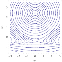
(a) $J_{1}=1.6$

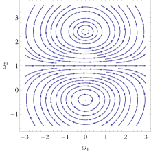
(b) $J_{1}=2.5$

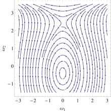
(c) $J_{1}=4$

Figure 1. Phase portraits of affine Suslov problem with $J_{2}\neq J_{1}$ and $J_{3}\neq J_{1}$. Values of parameters: $I_{22}=3$, $I_{33}=2$, $I_{23}=1/2$.

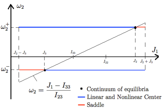
Figure 2. Bifurcation diagram under the assumption $J_{2}-J_{3}<J_{3}<I_{33}<I_{22}<J_{2}<J_{2}+J_{3}$. This is physically attainable (for example if $I_{22}=3,\,I_{33}=2,\,I_{23}=1/2$).

3.2. Suppose that $J_{1}=J_{2}$ or $J_{1}=J_{3}$.

Define the quantity

$$P=I_{23}^{2}-(J_{1}-I_{22})(J_{1}-I_{33}).$$ (3.5)

In view of (3.1), the condition that $J_{1}=J_{2}$ or $J_{1}=J_{3}$ is equivalent to saying that $P=0$. In this section we will also work under the assumption that $J_{1}\neq I_{33}$ because otherwise, the condition that $P=0$ implies $I_{23}=0$ that brings us back to the case discussed in Section 2. Therefore we can write

$$I_{22}=\frac{J_{1}^{2}-I_{23}^{2}-J_{1}I_{33}}{J_{1}-I_{33}}.$$ (3.6)

Under this assumption, $J_{1}$ is obviously a multiplicity two eigenvalue of the inertia tensor. The other eigenvalue of $I\mkern-7.0muI$ is given in terms of $J_{1},\,I_{33}$ and $I_{23}$ by

$$J_{0}=\frac{J_{1}^{2}-J_{1}I_{33}-I_{23}^{2}}{J_{1}-I_{33}}.$$ (3.7)

Substitution of (3.6) into (3.2) yields the following set of equations that possess a common factor

$$\omega^{\prime}_{1}=\dfrac{(I_{23}\omega_{2}+I_{33}-J_{1})(I_{33}\omega_{2}-J_{1}\omega_{2}-I_{23})}{J_{1}(J_{1}-I_{33})},\qquad\omega_{2}^{\prime}=\frac{(J_{1}-I_{33})\omega_{1}(I_{23}\omega_{2}+I_{33}-J_{1})}{J_{1}^{2}-I_{23}^{2}-J_{1}I_{33}}.$$ (3.8)

Notice that under our assumption that $J_{1}=J_{2}$ or $J_{1}=J_{3}$, the first integral (3.3) becomes indeterminate. However, in this case, there exists another one, quadratic in $\omega_{1}$ and $\omega_{2}$. We can obtain it using separation of variables in (3.8). Namely, we can write

$$\dfrac{\mathrm{d}\omega_{1}}{\mathrm{d}\omega_{2}}=\dfrac{(I_{33}\omega_{2}-J_{1}\omega_{2}-I_{23})(J_{1}^{2}-I_{23}^{2}-J_{1}I_{33})}{J_{1}(J_{1}-I_{33})^{2}\omega_{1}}.$$

Now we use separation of variables to get

$$J_{1}(J_{1}-I_{33})^{2}\omega_{1}\,\mathrm{d}\omega_{1}=(I_{33}\omega_{2}-J_{1}\omega_{2}-I_{23})(J_{1}^{2}-I_{23}^{2}-J_{1}I_{33})\,\mathrm{d}\omega_{2}$$

and we integrate both sides independently. After multiplication by two we obtain first integral

$$\tilde{G}(\omega_{1},\omega_{2})=J_{1}(J_{1}-I_{33})^{2}\omega_{1}^{2}+(J_{1}-I_{33})(J_{1}^{2}-I_{23}^{2}-J_{1}I_{33})\omega_{2}^{2}+2I_{23}(J_{1}^{2}-I_{23}^{2}-J_{1}I_{33})\omega_{2}.$$

Notice that the coefficient of $\omega_{2}^{2}$ can be written as $I_{22}(J_{1}-I_{33})^{2}$ and is therefore positive (since the matrix $I\mkern-7.0muI$ is positive definite). It follows that $\tilde{G}$ is positive definite and its level sets are ellipses in the $\omega_{1}\,\omega_{2}$ plane. In order to integrate the system explicitly we perform a change of variables that puts the equations in a simpler form. We introduce the variables $\xi,\eta$ by the relations

$$\omega_{1}=\frac{\xi}{I_{23}},\qquad\omega_{2}=\frac{\eta}{I_{23}}+\frac{J_{1}-I_{33}}{I_{23}}.$$ (3.9)

Then, the system (3.8) takes the form

$$\xi^{\prime}=-A(\eta-B)\eta,\qquad\eta^{\prime}=C\xi\eta,$$ (3.10)

where the constants $A,\,B,\,C$ are given by

$$A=\frac{1}{J_{1}},\qquad B=J_{0}-J_{1},\qquad C=\frac{1}{I_{22}},$$

with $I_{22}$ and $J_{0}$ given respectively by (3.6) and (3.7). The conserved quantity takes the simple form

$$G(\xi,\eta)=A(\eta-B)^{2}+C\xi^{2}.$$

Under our assumptions, we have $A,\,C>0$ and $B\neq 0$. Notice that, similar to the classical Suslov problem, the system (3.10) possesses a continuum of equilibrium points along the line $\eta=0$. On the other hand, the level sets of the conserved quantity $G$ are ellipses centered at the point $(0,B)$ in the $\xi\eta$ plane, that is itself another equilibrium of the system. The number of intersections of these ellipses with the line $\eta=0$ will depend on the specific value of $G$. Let

$$G_{0}=AB^{2}=\frac{(J_{0}-J_{1})^{2}}{J_{1}}>0.$$

Then,

1. For $0<G<G_{0}$ there are no intersections of the level sets of $G$ with the line $\eta=0$. The solutions are periodic and we shall see that they are expressed as a ratio of trigonometric functions.

2. The level set $G=G_{0}$ touches the line $\eta=0$ with multiplicity two at the equilibrium point $(0,0)$. The level set is an orbit homoclinic to $(0,0)$ and we will see that the solution along this orbit is a rational function of $\tau$.

3. For values $G>G_{0}$ the ellipses cut the line $\eta=0$ at the two equilibrium points $\left(\pm\sqrt{\frac{G-AB^{2}}{C}},0\right)$. The arcs of the ellipse connecting these points are two heteroclinic orbits. The solutions along these orbits are expressed in terms of hyperbolic functions.

The level set $G=0$ obviously consists of the individual equilibrium point $(0,B)$. A schematic picture of the phase portrait is shown in Figure 3 below under the assumption that $B>0$.

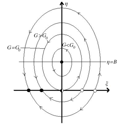
Figure 3. Schematic representation of the phase portrait of equations (3.10) under the assumption that $B>0$.

Explicit solutions to (3.10).

The dependence of $\xi$ and $\eta$ on $\tau$ along the contour line $G(\xi,\tau)=g$ can be obtained by introducing the parametrization:

$$\xi=\sqrt{\frac{g}{C}}\frac{2\psi}{\psi^{2}+1},\qquad\eta=\pm\sqrt{\frac{g}{A}}\left(\frac{1-\psi^{2}}{\psi^{2}+1}\right)+B.$$ (3.11)

Substitution into (3.10) yields the separable equation for $\psi(\tau)$

$$\psi^{\prime}=K_{1}\psi^{2}+K_{2}$$

for certain constants $K_{1}$ and $K_{2}$ that satisfy $\mbox{sign}(K_{1}K_{2})=\mbox{sign}(G_{0}-g)$. Hence, as expected, the form of the solutions will depend on how $g$ compares to $G_{0}=AB^{2}$.

For $0<g<G_{0}$ it is enough to consider one branch of the parametrization (3.11). Using the “-” branch and simplifying the algebra, one ends up with the explicit solution

$$\begin{split}\xi(\tau)&=\sqrt{\frac{g}{C}}\left(\frac{\sqrt{AB^{2}-g}\sin(\sqrt{C}\sqrt{AB^{2}-g}\,\tau)}{\sqrt{A}B+\sqrt{g}\cos(\sqrt{C}\sqrt{AB^{2}-g}\,\tau)}\right),\\ \eta(\tau)&=-\sqrt{\frac{g}{A}}\left(\frac{\sqrt{g}+\sqrt{A}B\cos(\sqrt{C}\sqrt{AB^{2}-g}\,\tau)}{\sqrt{A}B+\sqrt{g}\cos(\sqrt{C}\sqrt{AB^{2}-g}\,\tau)}\right)+B.\end{split}$$

If $g=G_{0}=AB^{2}$ the same substitution yields the solution

$$\xi(\tau)=\frac{-2AB^{2}\tau}{ACB^{2}\tau^{2}+1},\qquad\eta(\tau)=\frac{2B}{ACB^{2}\tau^{2}+1}.$$

For values of $g$ bigger than $G_{0}=AB^{2}$ one needs to consider both branches of the parametrization to account for the two heteroclinic connections. The solution along the branch on the positive $\eta$-plane is given by

$$\begin{split}\xi(\tau)&=-\sqrt{\frac{g}{C}}\left(\frac{\sqrt{g-AB^{2}}\sinh(\sqrt{C}\sqrt{g-AB^{2}}\,\tau)}{-\sqrt{A}B+\sqrt{g}\cosh(\sqrt{C}\sqrt{g-AB^{2}}\,\tau)}\right),\\ \eta(\tau)&=\sqrt{\frac{g}{A}}\left(\frac{\sqrt{g}-\sqrt{A}B\cosh(\sqrt{C}\sqrt{g-AB^{2}}\,\tau)}{-\sqrt{A}B+\sqrt{g}\cosh(\sqrt{C}\sqrt{g-AB^{2}}\,\tau)}\right)+B.\end{split}$$

whereas the solution along the negative $\eta$-plane is given by

$$\begin{split}\xi(\tau)&=-\sqrt{\frac{g}{C}}\left(\frac{\sqrt{g-AB^{2}}\sinh(\sqrt{C}\sqrt{g-AB^{2}}\,\tau)}{\sqrt{A}B+\sqrt{g}\cosh(\sqrt{C}\sqrt{g-AB^{2}}\,\tau)}\right),\\ \eta(\tau)&=-\sqrt{\frac{g}{A}}\left(\frac{\sqrt{g}+\sqrt{A}B\cosh(\sqrt{C}\sqrt{g-AB^{2}}\,\tau)}{\sqrt{A}B+\sqrt{g}\cosh(\sqrt{C}\sqrt{g-AB^{2}}\,\tau)}\right)+B.\end{split}$$

4. Painlevé property of the solutions

In this section we continue analyzing the system (1.3) under the assumption $I_{13}=0$ that, as explained before, physically corresponds to the supposing that the vector $\bf a$ is orthogonal to a principal axis of inertia of the body. We shall prove

Theorem 4.1.

All solutions of equations (3.2) are single valued if and only if either $I_{23}=0$, or the eigenvalue $J_{1}=I_{11}$ coincides with $J_{2}$ or $J_{3}$ (see equation (3.1)).

Proof.

In Section 2 we proved that if $I_{23}=0$ then the equations become linear and homogeneous. On the other hand, in Section 3.2, where the assumption that $J_{1}=J_{2}$ or $J_{1}=J_{3}$ was made, we gave explicit meromorphic expressions for all the solutions. Hence, the only thing that remains to prove is that the system (3.2) has multi-valued solutions in the case considered in Section 3.1 (where $I_{23}\neq 0$ and $J_{1}\neq J_{2},J_{3}$).

If we transform system (1.3) into a second order equation, then we obtain

$$\omega_{2}^{\prime\prime}=\dfrac{I_{23}(\omega_{2}^{\prime})^{2}}{I_{23}\omega_{2}+I_{33}-J_{1}}+\dfrac{1}{J_{1}I_{22}}(J_{1}-I_{33}-I_{23}\omega_{2})[(I_{33}-I_{22})\omega_{2}+I_{23}(\omega_{2}^{2}-1)],$$

or

$$\eta^{\prime\prime}=\frac{(\eta^{\prime})^{2}}{\eta}+\frac{1}{J_{1}I_{22}}\eta[-\eta^{2}+(I_{22}+I_{33}-2J_{1})\eta+I_{23}^{2}-(J_{1}-I_{22})(J_{1}-I_{33})],$$ (4.1)

where, just like in (3.9), we have

$$\eta=I_{23}\omega_{2}+I_{33}-J_{1}.$$

We rewrite equation (4.1) in terms of the independent complex variable $\tau=z$ in the form

$$\frac{\mathrm{d}^{2}\eta}{\mathrm{d}z^{2}}=\frac{1}{\eta}\left(\frac{\mathrm{d}\eta}{\mathrm{d}z}\right)^{2}+p_{3}\eta^{3}+p_{2}\eta^{2}+p_{1}\eta.$$ (4.2)

Note that, up to a non-vanishing factor, the coefficient $p_{1}$ coincides with $P$ defined by (3.5). Recall that the condition that $P=0$ is equivalent to saying that $J_{1}$ coincides with $J_{2}$ or $J_{3}$. Hence, by our analysis in Section 3.2 we conclude that if $p_{1}=0$ all solutions are single-valued. We note in passing that in this case  (4.1) takes the form of equation XII in Painlevé-Gambier classification [3, 2] that is well-known to have all solutions single-valued.

We shall now prove that if $p_{1}\neq 0$, there exists a solution to (4.2) with a movable logarithmic singular point. We apply the $\alpha$-method of Painlevé, see Chapter XIV in [3]. Let us introduce new variables

$$\eta=\frac{1}{\alpha}u,\qquad z=\alpha\zeta.$$

The transformed equation reads

$$\frac{\mathrm{d}^{2}u}{\mathrm{d}\zeta^{2}}=\frac{1}{u}\left(\frac{\mathrm{d}u}{\mathrm{d}\zeta}\right)^{2}+p_{3}u^{3}+\alpha p_{2}u^{2}+\alpha^{2}p_{1}u.$$

It has a solution of the form

$$u(\zeta)=u_{0}(\zeta)+\alpha u_{1}(\zeta)+\alpha^{2}u_{2}(\zeta)+\cdots,$$

where the dots denote higher order terms. If all solutions of equation (4.2) are single valued, then $u_{i}(\zeta)$ must be single valued for all $i\geq 0$. The function $u_{0}(\zeta)$ is a solution of the equation

$$\frac{\mathrm{d}^{2}u_{0}}{\mathrm{d}\zeta^{2}}=\frac{1}{u_{0}}\left(\frac{\mathrm{d}u_{0}}{\mathrm{d}\zeta}\right)^{2}+p_{3}u_{0}^{3}.$$ (4.3)

On the other hand, the functions $u_{i}(\zeta)$ with $i>0$ are solutions of the following linear non-homogeneous equations

$$u_{i}^{\prime\prime}=\frac{2u_{0}^{\prime}(\zeta)}{u_{0}(\zeta)}u_{i}^{\prime}+\left[3p_{3}u_{0}(\zeta)^{2}-\left(\frac{u_{0}^{\prime}(\zeta)}{u_{0}(\zeta)}\right)^{2}\right]u_{i}+b_{i}(\zeta),$$ (4.4)

where $b_{1}(\zeta):=p_{2}u_{0}(\zeta)^{2}$, and

$$b_{2}:=u_{0}\left(p_{1}+2p_{2}u_{1}+3p_{3}u_{1}^{2}\right)+\frac{u_{0}^{\prime 2}u_{1}^{2}}{u_{0}^{3}}-2\frac{u_{0}^{\prime}u_{1}u_{1}^{\prime}}{u_{0}^{2}}+\frac{u_{1}^{\prime 2}}{u_{0}}.$$

In general $b_{i}$ will depend on $u_{j}$ with $j<i$.

Let $v_{1}$ and $v_{2}$ be linearly independent solutions of homogeneous part of equation (4.4) and $V$ its fundamental matrix, i.e.,

$$V=\begin{bmatrix}v_{1}&v_{2}\\ v_{1}^{\prime}&v_{2}^{\prime}\end{bmatrix}.$$

Then, the solution of (4.4) is given by

$$\begin{bmatrix}u_{i}(\zeta)\\ u_{i}^{\prime}(\zeta)\end{bmatrix}=V(\zeta)\int^{\zeta}V^{-1}(x)\begin{bmatrix}0\\ b_{i}(x)\end{bmatrix}\,\mathrm{d}x.$$

The general solution of equation (4.3) has the form

$$u_{0}(\zeta)=\frac{2a^{2}\exp[a\zeta+b]}{\exp[2(a\zeta+b)]-a^{2}p_{3}}.$$

It has a simple pole at point $\zeta=c$ where $c$ is defined by the condition

$$\exp[2(ac+b)]=a^{2}p_{3}.$$

It follows that if the solutions of (4.4) have a branch points, then they are located either at $\zeta=c$ or at infinity.

It is easy check that $u_{1}(\zeta)$ is always single valued but

$$\operatorname{residue}\left(V^{-1}(\zeta)\begin{bmatrix}0\\ b_{2}(\zeta)\end{bmatrix},c\right)=\begin{bmatrix}-2\exp(-ac-b)p_{1}\\ \exp(-ac-b)p_{1}\end{bmatrix}.$$

Thus, if $p_{1}\neq 0$ then logarithmic terms are present. This completes the proof. ∎

References

• [1] Borisov A V, Mamaev I S and Kilin A A
Hamiltonicity and integrability of the Suslov problem Regul. Chaotic Dyn. 16 (2011), 104–116.
• [2] Gambier B
Sur les équations différentielles du second ordre et du premier degré dont l’intégrale générale est à points critiques fixes Acta Math. 33 (1910), 1–55.
• [3] Ince, E. L.
Ordinary Differential Equations, New York, Ordinary Differential Equations, 1944.
• [4] Fedorov Y N, Maciejewski A J and Przybylska M
The Poisson equations in the nonholonomic Suslov problem: integrability, meromorphic and hypergeometric solutions Nonlinearity 22 (2009), 2231–2259.
• [5] Painlevé P
Mémoire sur les équations différentielles dont l’intégrale générale est uniforme, Bulletin de la S. M. F. 28 (1900), 201–261.
• [6] Painlevé P
Sur les équations différentielles du second ordre et d’ordre supérieur dont l’intégrale générale est uniforme Acta Math. 25 (1902), 1–85.
• [7] Suslov, G. K
Theoretical Mechanics, Moscow, Gostekhizdat, 1946 (Russian).