The HST/ACS Coma Cluster Survey - VII. Structure and Assembly of Massive Galaxies in the Center of the Coma Cluster

Abstract

We constrain the assembly history of galaxies in the projected central 0.5 Mpc of the Coma cluster by performing structural decomposition on 69 massive ($M_{\star}\geq 10^{9}$ $M_{\odot}$) galaxies using high-resolution F814W images from the HST Treasury Survey of Coma. Each galaxy is modeled with up to three Sérsic components having a free Sérsic index $n$. After excluding the two cDs in the projected central 0.5 Mpc of Coma, 57% of the galactic stellar mass in the projected central 0.5 Mpc of Coma resides in classical bulges/ellipticals while 43% resides in cold disk-dominated structures. Most of the stellar mass in Coma may have been assembled through major (and possibly minor) mergers. Hubble types are assigned based on the decompositions, and we find a strong morphology-density relation; the ratio of (E+S0):spirals is (91.0%):9.0%. In agreement with earlier work, the size of outer disks in Coma S0s/spirals is smaller compared with lower-density environments captured with SDSS (Data Release 2). Among similar-mass clusters from a hierarchical semi-analytic model, no single cluster can simultaneously match all the global properties of the Coma cluster. The model strongly overpredicts the mass of cold gas and underpredicts the mean fraction of stellar mass locked in hot components over a wide range of galaxy masses. We suggest that these disagreements with the model result from missing cluster physics (e.g., ram-pressure stripping), and certain bulge assembly modes (e.g., mergers of clumps). Overall, our study of Coma underscores that galaxy evolution is not solely a function of stellar mass, but also of environment.

1 Introduction

How galaxies form and evolve is one of the primary outstanding problems in extragalactic astronomy. The initial conditions led to the collapse of dark matter halos which clustered hierarchically into progressively larger structures. In the halo interiors, gas formed rotating disks which underwent star formation (SF) to produce stellar disks (Cole 2000; Steinmetz & Navarro 2002). The subsequent growth of galaxies is thought to have proceeded through a combination of major mergers, (e.g., Toomre 1977; Barnes 1988; Khochfar & Silk 2006, 2009), minor mergers (e.g., Oser et al. 2012, Hilz et al. 2013), cold-mode gas accretion (Birnboim & Dekel 2003; Kereš et al. 2005, 2009; Dekel & Birnboim 2006; Brooks et al. 2009; Ceverino et al. 2010; Dekel et al. 2009a, b), and secular processes (Kormendy & Kennicutt 2004).

In early simulations focusing on gas-poor mergers, the major merger of two spiral galaxies with mass ratio $M_{1}/M_{2}\geq 1/4$ would inevitably destroy the pre-existing stellar disks by violent relaxation, producing a remnant bulge or elliptical having a puffed-up distribution of stars with a low ratio of ordered-to-random motion ($V/\sigma$) and a steep de Vaucouleurs $r^{1/4}$ surface brightness profile (Toomre 1977). Improved simulations (Robertson et al. 2006; Naab et al. 2006; Governato et al. 2007; Hopkins et al. 2009a, b) significantly revised this picture. In unequal-mass major mergers, violent relaxation of stellar disks is not complete. Furthermore, for major mergers where the progenitors have moderate-to-high gas fractions, gas-dissipative processes build disks on small and large scales (Hernquist & Mihos 1995; Robertson et al. 2006; Hopkins et al. 2009a, b; Kormendy et al. 2009). The overall single Sérsic index $n$ of such remnants are typically $2\lesssim n\lesssim 4$ (Naab et al. 2006; Naab & Trujillo 2006; Hopkins et al. 2009a). The subsequent accretion of gas from the halo, cold streams, and minor mergers can further build large-scale stellar disks, whose size depends on the specific angular momentum of the accreted gas (Steinmetz & Navarro 2000; Birnboim & Dekel 2003; Kereš et al. 2005, 2009; Dekel & Birnboim 2006; Robertson et al. 2006; Dekel et al. 2009a, b; Brooks et al. 2009; Hopkins et al. 2009b; Ceverino et al. 2010). Additionally, Bournaud, Elmegreen, & Elmegreen (2007) and Elmegreen et al. (2009) discuss bulge formation via the merging of clumps forming within very gas-rich, turbulent disk in high-redshift galaxies. These bulges can have a range of Sérsic indices, ranging from $n<2$ to $n=4$.

As far as the structure of galaxies is concerned, we are still actively studying and debating the epoch and formation pathway for the main stellar components of galaxies, namely flattened, dynamically cold, disk-dominated components (including outer disks, circumnuclear disks, and pseudobulges) versus puffy, dynamically hot spheroidal or triaxial bulges/ellipticals. Getting a census of dynamically hot bulges/ellipticals and dynamically cold, flattened disk-dominated components on large and small scales in galaxies provides a powerful way of evaluating the importance of violent bulge-building processes, such as violent relaxation, versus gas-dissipative disk-building processes.

We adopt throughout this paper the widely used definition of a bulge as the excess light above an outer disk in an S0 or spiral galaxy (e.g., Laurikainen et al. 2007, 2009, 2010; Fisher & Drory 2008; Gadotti 2009; Weinzirl et al. 2009). The central bulge falls in three main categories called classical bulges, disky pseudobulges (Kormendy 1993; Kormendy & Kennicutt 2004; Jogee, Scoville, & Kenney 2005; Athanassoula 2005; Kormendy & Fisher 2005; Fisher & Drory 2008), and boxy pseudobulges (Combes & Sanders 1981; Combes et al. 1990; Pfenniger & Norman 1990; Bureau & Athanassoula 2005; Athanassoula 2005; Martinez-Valpuesta et al. 2006). Some bulges are composite mixtures of the first two classes (Kormendy & Barentine 2010; Barentine & Kormendy 2012). For remainder of the paper we refer to classical bulges simply as “bulges” when the context is unambiguous.

Numerous observational efforts have been undertaken to derive such a census among galaxies in the field environment. Photometric studies (e.g., Kormendy 1993; Graham 2001; Balcells et al. 2003, 2007b; Laurikainen et al. 2007; Graham & Worley 2008; Fisher & Drory 2008; Weinzirl et al. 2009; Gadotti 2009; Kormendy et al. 2010) have dissected field galaxies into outer stellar disks and different types of central bulges (classical, disky/boxy pseudobulges) associated with different Sérsic index, and compiled the stellar bulge-to-total light or mass ratio ($B/T$) of spirals and S0s. It is found that low-$B/T$ and bulgeless galaxies are common in the field at low redshifts, both among low-mass or late-type galaxies (Böker et al. 2002; Kautsch et al. 2006; Barazza et al. 2007, 2008) and among high-mass spirals or early-type spirals (Kormendy 1993; Balcells et al. 2003, 2007b; Laurikainen et al. 2007; Graham & Worley 2008; Weinzirl et al. 2009; Gadotti 2009; Kormendy et al. 2010). Balcells et al. (2003) highlighted the paucity of $r^{1/4}$ profiles in the bulges of early-type disk galaxies. Working on a bigger sample, Weinzirl et al. (2009) report that the majority ($66.4\pm 4.4\%$) of massive ($M_{\star}\geq 10^{10}$ $M_{\odot}$) field spirals have low $B/T$ ($\leq 0.2$) and bulges with low Sérsic index ($n\leq 2$).

These empirical results can be used to test models of the assembly history of field galaxies. For instance, Weinzirl et al. (2009) find that the results reported above are consistent with hierarchical semi-analytic models of galaxy evolution from Khochfar & Silk (2006) and Hopkins et al. (2009a), which predict that most ($\sim 85\%$) massive field spirals have had no major merger since $z=2$. While this work reduces the tension between theory and observations for field galaxies, one should note that hydrodynamical models still face challenges in producing purely bulgeless massive galaxies in different environments.

It is important to extend such studies from the field environment to rich clusters. Hierarchical models predict differences in galaxy merger history as a function of galaxy mass, environment, and redshift (Cole et al. 2000; Khochfar & Burkert 2001). Furthermore, cluster-specific physical processes, such as ram-pressure stripping (Gunn & Gott 1972; Fujita & Nagashima 1999), galaxy harassment (Barnes & Hernquist 1991; Moore et al. 1996, 1998, 1999; Hashimoto et al. 1998; Gnedin 2003), and strangulation (Larson et al. 1980), can alter SF history and galaxy stellar components (disks, bulges, bars).

Efforts to establish accurate demographics of galaxy components in clusters are ongoing. In the nearby Virgo cluster, Kormendy et al. (2009) find more than 2/3 of the stellar mass is in classical bulges/ellipticals, including the stellar mass contribution from M87. Furthermore, there is clear evidence for ongoing environmental effects in Virgo; see Kormendy & Bender (2012) for a comprehensive review.

Yet Virgo is not very rich compared with more typical clusters (Heiderman et al. 2009). The Coma cluster at $z=0.024$ ($D=100$ Mpc) has a central number density 10,000 Mpc^-3 (The & White 1986) and is the densest cluster in the local universe. However, ground-based data do not provide high enough resolution ($1^{\prime\prime}-2^{\prime\prime}=500-1000$ pc) for accurate structural decomposition, an obstacle to earlier work.

In this paper we make use of data from the $Hubble$ $Space$ $Telescope$ (HST) Treasury Survey (Carter et al. 2008) of Coma which provides high-resolution (50 pc) imaging from the Advanced Camera for Surveys (ACS). Our goal is to derive the demographics of galaxy components, in particular classical bulges/ellipticals and flattened disk-dominated components (including both large-scale disks and disky pseudobulges), in the Coma cluster, and to compare the results with lower-density environments and to theoretical models, to constrain the assembly history of galaxies.

In Section 2 we present our mass-complete sample of cluster galaxies with stellar mass $M_{\star}\geq 10^{9}$ $M_{\odot}$. In Section 3 we describe our structural decomposition strategy. Section 3.1 describes our working assumption in this paper of using Sérsic index as a proxy for tracing the disk-dominated structures and classical bulges/ellipticals. Section 3.2 outlines our procedure for structural decomposition, and we refer the reader to Appendix A for a more detailed description. Section 3.3 overviews the scheme we use to assign morphological types to galaxies. In Section 4.1, we quantitatively assign galaxy types based on the structural decompositions. We also make a census (Section 4.2) of structures built by dissipation versus violent stellar processes, explore how stellar mass is distributed in different galaxy components (Section 4.3), and consider galaxy scaling relations (Section 4.4). In Section 4.5, we evaluate and discuss the effect of cluster environmental processes. In Section 5 we compare our empirical results with theoretical models, after first identifying Coma-like environments in the simulations. Readers not interested in the complete details about the theoretical model can skip to Sections 5.3 and 5.6. We summarize our results in Section 6.

We adopt a flat $\Lambda$CDM cosmology with $\Omega_{\Lambda}=0.7$ and $H_{0}=73$ km s^-1 Mpc^-1. We use AB magnitudes throughout the paper, except where indicated otherwise.

2 Data and Sample Selection

This study is based on the data products from the HST/ACS Coma Cluster Treasury Survey (Carter et al. 2008), which provides ACS Wide Field Camera images for 25 pointings spanning 274 arcmin² in the F475W and F814W filters. The total ACS exposure time per pointing is typically 2677 seconds in F475W and 1400 seconds in F814W. Most (19/25) pointings are located within 0.5 Mpc from the central cD galaxy NGC 4874, and the other 6/25 pointings are between 0.9 and 1.75 Mpc southwest of the cluster center. The FWHM of the ACS point-spread function (PSF) is $\sim 0\hbox{$.\!\!^{\prime\prime}$}1$ (Hoyos et al. 2011), corresponding to $\sim 50$ pc at the 100 Mpc distance of the Coma cluster (Carter et al. 2008). Note the 19 pointings cover only $19.7\%$ by area of the projected central 0.5 Mpc of Coma. This limited spatial coverage of ACS in the projected central 0.5 Mpc of Coma may introduce a possible bias in the sample due to cosmic variance. We quantify this effect in Appendix B.5 and discuss the implications throughout the paper.

Hammer et al. (2010) discuss the images and SExtractor source catalogs for Data Release 2.1 (DR2.1). The F814W $5\sigma$ limit for point sources is 26.8 mag (Hammer et al. 2010), and we estimate the $5\sigma$ F814W surface brightness limit for extended sources within a $0\hbox{$.\!\!^{\prime\prime}$}7$ diameter aperture to be 25.6 mag/arcsec². Several of the ACS images in DR2.1 suffer from bias offsets on the inter-chip and/or inter-quadrant scale that cause difficulty in removing the sky background. We use the updated ACS images reprocessed to reduce the impact of this issue. The DR2.1 images are used where this issue is not present.

2.1 Selection of Bright Cluster Members

We select our sample based on the eyeball catalog of N. Trentham et al. (in preparation), with updates from Marinova et al. (2012). This catalog provides visually determined morphologies and cluster membership status for galaxies with an apparent magnitude F814W $\leq 24$ mag. Morphology classifications in this catalog come from a combination of RC3 (de Vaucouleurs et al. 1991) and visual inspection. In Section 4.1 we assign Hubble types based only on our own multi-component decompositions.

Cluster membership is ranked from 0 to 4 following the method of Trentham & Tully (2002). Membership class 0 means the galaxy is a spectroscopically confirmed cluster member. The subset of spectroscopically confirmed cluster members was identified based on published redshifts (Colless & Dunn 1996; Adelman-McCarthy et al. 2008; Mobasher et al. 2001; Chiboucas et al. 2010) and is approximately complete in surface brightness at the galaxy half-light radius ($\mu_{\mathrm{e,F814W}}$) to $\sim 22.5$ mag/arcsec² (den Brok et al. 2011). The remaining galaxies without spectroscopic confirmation are assigned a rating of 1 (very probable cluster member), 2 (likely cluster member), 3 (plausible cluster member), or 4 (likely background object) based on a visual estimation that also considers surface brightness and morphology.

From this catalog, we define a sample S1 of 446 cluster members having F814W $\leq 24$ mag and membership rating 0-3 located within the projected central 0.5 Mpc of Coma, which is the projected radius probed by the central ACS pointings. To S1 we add the second central cD galaxy NGC 4889, which is not observed by the ACS data. The majority (179) of S1 galaxies have member class 0, and 30, 131, and 106 have member class 1, 2, and 3, respectively.

2.2 Calculation of Stellar Masses

Stellar masses are a thorny issue. Uncertainties in the mass-to-light ratios of stellar populations ($M/L$) arise from a poorly known initial mass function (IMF) as well as degeneracies between age and metallicity. We calculate stellar masses based on the $HST$ F475W and F814W-band photometry. First, we convert the $HST$ (AB) photometry to the Cousins-Johnson (Vega) system using

$$\rm{I=F814W-0.38}$$ (1)

from the WFPC2 Photometry Cookbook and

$$\rm{B-I=1.287\left(F475W-F814W\right)+0.538}$$ (2)

from Price et al. (2009).

Next, we calculate $I$-band $M/L$ from the calibrations of Into & Portinari (2013) for a Kroupa et al. (1993) initial mass function (IMF) with

$$\rm{I_{lum}=10^{\left(-0.4\left(I-35-4.08\right)\right)}}$$ (3)

and

$$\rm{M_{\star}=I_{lum}\times 10^{\left(0.641\left(B-I\right)-0.997\right)}},$$ (4)

where $I$ corresponds to the apparent MAG_AUTO SExtractor magnitude, 35 is the distance modulus to Coma, and 4.08 is the solar absolute magnitude in $I$-band.

We use the above method to calculate stellar masses for all galaxies in S1 except NGC 4889, which does not have ACS data. For NGC 4889, we use $gr$ Petrosian magnitudes from SDSS DR10 (Ahn et al. 2013). Stellar masses are determined using the relations of Bell et al. (2003) and assuming a Kroupa IMF, namely

$$\rm{g_{lum}=10^{\left(-0.4\left(g-35-5.10\right)\right)}}$$ (5)

and

$$\rm{M_{\star}=g_{lum}\times 10^{\left(-0.499+1.519\left(g-r\right)-0.1\right)}},$$ (6)

where $g$ and $r$ are apparent SDSS magnitudes, 35 is the distance modulus to Coma, and 5.10 is the solar absolute magnitude in $g$-band.

It is hard to derive the stellar mass of cD galaxies for several reasons. The stellar $M/L$ ratio of cDs is believed to be high ($M_{\rm dyn}/L_{B}>100$; Schneider 2006), but is very uncertain as most of the light of a cD is in an outer envelope made of intra-cluster light and galaxy debris. Another problem is that even if one knew the correct stellar $M/L$ ratio, it is likely that the available photometry from ACS and SDSS is missing light from the extended low surface brightness envelope. Given all these factors, it is likely that the above equations, which are typically used to convert color to $M_{\star}$ for normal representative galaxies, are underestimating the $M/L$ ratios and stellar masses of the cDs, so that the adopted stellar masses for the cDs ($M_{\star}\sim 6-8\times 10^{11}$ $M_{\odot}$) are lower limits. Due to the uncertain stellar masses of the cDs, we present many of our results without them, and we take care to consider them separately from the less massive galaxy population of E, S0, and spiral galaxies.

2.3 Selection of Final Sample of Massive Galaxies

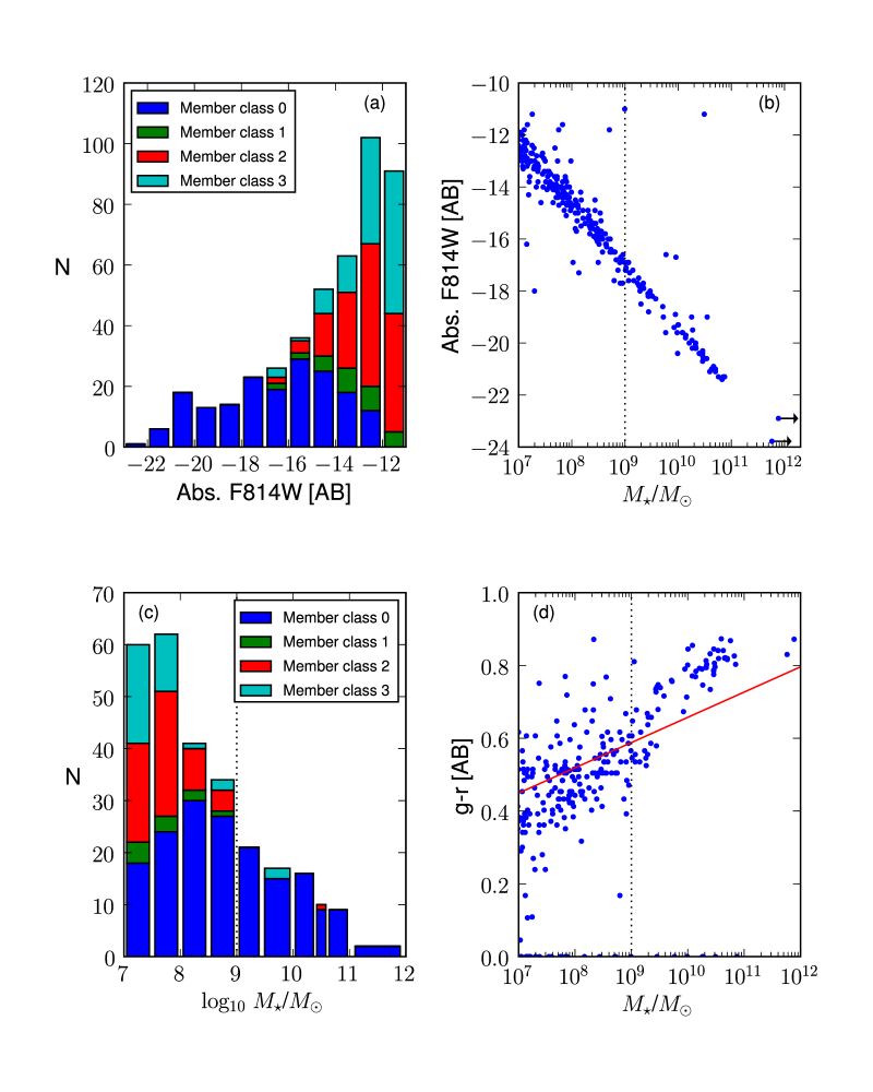
Figure 1: This figure shows in panels (a) to (d) the luminosity, stellar mass, and $g-r$ color, respectively, for the 446 galaxies in sample S1 having F814W$\leq 24$, locations within the projected central 0.5 Mpc of the Coma cluster, and cluster membership rating 0-3, where rating 0 means spectroscopically confirmed and rating 1-3 indicate increasingly less likely cluster membership. See Section 2.1 for details. In panel (b), the two most massive sources are cD galaxies, and the arrows indicate their adopted stellar masses are lower limits (Section 2.2). The solid line in panel (d) is the color-luminosity break between the red and blue sequence of galaxies from Blanton et al. (2005), which we convert from luminosity to stellar mass using the relations of Bell et al. (2003). The dotted line in panels (b)-(d) indicates our main sample of 69 spectroscopically confirmed members with $M_{\star}\geq 10^{9}$ $M_{\odot}$.

The left panels of Figure 1 show the distributions of F814W magnitudes (upper panel) and stellar masses (lower panels) for sample S1, while in the right panels of the same figure the correlations of stellar masses with F814W magnitudes (upper panel) and $g-r$ colors (lower panel) are shown.

In this paper, we focus on massive ($M_{\star}\geq 10^{9}$ $M_{\odot}$) galaxies. Our rationale is that we are specifically interested in understanding the evolution of the most massive cluster galaxies through comparisons with model clusters (Section 5) which show mass incompleteness at galaxy stellar masses $M_{\star}<10^{9}$ $M_{\odot}$. We found for sample S1 that imposing the mass cut  $M_{\star}\geq 10^{9}$ $M_{\odot}$ effectively removes most galaxies identified in the Trentham et al. catalog as dwarf/irregular and very low surface brightness galaxies. With this cut, we are left with 75 galaxies that consist primarily of E, S0, and spiral galaxies, two cDs, and only six dwarfs. Three out of 75 galaxies are significantly cutoff the ACS detector, and we ignore these sources. Of the remaining 72 galaxies, 69/72 have spectroscopic redshifts. The 3/72 galaxies without spectroscopic redshifts appear too red to be in Coma (Figure 1d), and the estimated SDSS DR10 photometric redshifts are much larger than the redshift of Coma (0.024). We also neglect these three sources as they are unlikely to be Coma members. Our final working sample S2 consists of the 69 galaxies inside the projected central 0.5 Mpc with stellar mass $M_{\star}\geq 10^{9}$ $M_{\odot}$ and spectroscopic redshifts. Table 1 cross references our sample with other datasets.

3 Method and Analysis

3.1 Using Sérsic Index as a Proxy For Tracing Disk-Dominated Structures and Classical Bulges/Ellipticals

As outlined in Section 1, galaxy bulges and stellar disks hold information on galaxy assembly history. The overall goal in this work is to separate galaxy components into groups of classical bulges/ellipticals versus disk-dominated structures.

It is common practice (e.g., Laurikainen et al. 2007; Gadotti 2009; Weinzirl et al. 2009) to characterize galaxy structures (bulges, disks, and bars) with generalized ellipses whose radial light distributions are described by the Sérsic (1968) profile:

$$\rm{I(r)=I_{e}\ exp\left(-b_{n}\left[\left(r\over{r_{\mathrm{e}}}\right)^{1/n}-1\right]\right)},$$ (7)

where $I_{e}$ is the surface brightness at the effective radius $r_{\mathrm{e}}$ and $b_{n}$ is a constant that depends on Sérsic index $n$.

In this paper, we adopt the working assumption that in intermediate and high-mass ($M_{\star}\geq 10^{9}$ $M_{\odot}$) galaxies, a low Sérsic index $n$ below a threshold value $n_{\rm disk\_max}$ corresponds to a dynamically cold disk-dominated structure. Note we specify “disk-dominated” rather than “pure disk” as we refer to barred disks and thick disks. While this assumption is not necessarily waterproof, it is based on multiple lines of compelling evidence that are outlined below.

1. Freeman (1970) showed that many large-scale disks of S0 and spiral galaxies are characterized by an exponential light profile (Sérsic index $n=1$) over 4-6 disk scalelengths. Since then, it has become standard practice in studies of galaxy structure to model the outer disk of S0s and spirals with an exponential profile (e.g., Kormendy 1977; Boroson 1981; Kent 1985; de Jong 1996; Baggett et al. 1998; Byun & Freeman 1995; Allen et al. 2006; Laurikainen 2007; Gadotti 2009; Weinzirl et al. 2009).

2. On smaller scales, flattened, rotationally supported inner disks with high $V/\sigma$ (i.e., disky pseudobulges) have been associated with low Sérsic index $n\lesssim 2$ (Kormendy 1993; Kormendy & Kennicutt 2004; Jogee, Scoville, & Kenney 2005; Athanassoula 2005; Kormendy & Fisher 2005; Fisher & Drory 2008; Fabricius et al. 2012). This suggests $n_{\rm disk\_max}$ should be close to 2.

   Fabricius et al. (2012) explore the major-axis kinematics of 45 S0-Scd galaxies with high-resolution spectroscopy. They demonstrate a systematic agreement between the shape of the velocity dispersion profile and the bulge type as indicated by the Sérsic index. Low Sérsic index bulges have both increased rotational support (higher $<V^{2}>/<\sigma^{2}>$ values) and on average lower central velocity dispersions. Classical bulges (disky pseudobulges) show have centrally peaked (flat) velocity dispersion profiles whether identified visually or by a high Sérsic index.

3. At high ($z\sim 2$) redshift, where it is not yet possible to fully resolve galaxy substructures, it has become conventional to use the global Sérsic index $n\lesssim 2$ in massive galaxies to separate disk-dominated versus bulge-dominated galaxies (e.g., Ravindranath et al. 2004; van der Wel et al. 2011; Weinzirl et al. 2011). Weinzirl et al. (2011) further explore the distributions of ellipticities ($1-b/a$) for the massive $z\sim 2$ galaxies with low ($n\leq 2$) and high ($n>2$) global Sérsic index. They find galaxies with low global Sérsic index $n\leq 2$ have a distribution of projected ellipticities more similar to massive $z\sim 0$ spirals than to massive $z\sim 0$ ellipticals.

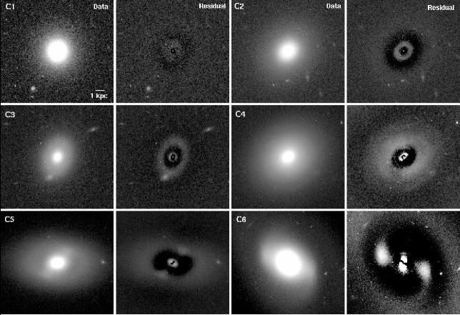
Figure 15: This figure shows examples C1 to C6 where a single Sérsic model (plus point source if needed) does not provide a good fit to coherent galaxy structure that is best modeled with one or more additional Sérsic profiles. Such residual structure includes central compact structures (C2, C3, C4, C5, C6), rings (C3, C4), annuli and extended components (C1, C4), and bars/ovals (C5, C6). These systems are better fitted by models with multiple Sérsic components (see Figures 16 and 17). Columns 1 and 3 show the input $I$-band images. Columns 2 and 4 show the residuals after subtracting the best single Sérsic fit. Note C1$=$COMAi125931.893p275140.76, C2$=$COMAi125935.286p275149.13, C3$=$COMAi13021.673p275354.81, C4$=$COMAi13014.746p28228.69, C5$=$COMAi13027.966p275721.56, and C6$=$COMAi125930.824p275303.05.

The above does not allow for low-$n$, dynamically hot structures. A low-$n$ dynamically hot structure would be considered in our study as a pure photometric disk, a low-$n$ bulge, or an unbarred S0 galaxy. The error due to misunderstood objects in the first two groups is expected to be small or nonexistent. There is only one pure photometric disk in the sample (Section 4.1) and low-$n$ bulges ($N=20$) only make up 2.2% of galaxy stellar mass (excluding the cDs, Section 4.2). Furthermore, Figure 15 of Fabricius et al. (2012) shows that no low-$n$ bulge turns out to be dynamically hot.

There are 20 unbarred S0 galaxies in our sample, and these account for 18.5% of the galaxy stellar mass (excluding the cD galaxies). About 75% of these objects have stellar mass and luminosity consistent with dwarf spheroidal galaxies (Kormendy et al. 2009). Even if some of these systems are actually dwarf spheroidals, they may not be dynamically hot as some studies (e.g., Kormendy et al. 2009, Kormendy & Bender 2012) claim that many dwarfs are actually disk systems closely related to dIrr, which have been stripped of gas via supernova feedback or environmental effects. The remaining 25% would be misclassified elliptical galaxies as they are too bright and massive to be dwarfs. Note, however, that Figure 33 of Kormendy et al. (2009) shows that elliptical galaxies with $M_{V}<-18$ and Sérsic $n<2$ are very rare. In the worse-case scenario that all of our unbarred S0 galaxies are dynamically hot structures, our measurement of the dynamically hot stellar mass in Section 4.2 would be too low by $\sim 30\%$.

The second natural related working assumption in our paper is that in intermediate and high-mass ($M_{\star}\geq 10^{9}$ $M_{\odot}$) galaxies, components with Sérsic $n>n_{\rm disk\_max}$ are classical bulge/elliptical components (defined in Section 1). Such bulges/ellipticals are formed by the redistribution of stars during major and minor galaxy collisions. $N$-body simulations show that minor mergers consistently raise the bulge Sérsic index (Aguerri et al. 2001; Eliche-Moral et al. 2006; Naab & Trujillo 2006). The effect of successive minor mergers is cumulative (Aguerri et al. 2001; Bournaud, Jog, & Combes 2007; Naab et al. 2009; Hilz et al. 2012).

We empirically set $n_{\rm disk\_max}$ to 1.66 based on looking at the Sérsic $n$ of outer disks in those Coma galaxies that are barred, and by definition, must harbor outer disk since bars are disk features. Appendix B.2 and Appendix D discuss the empirical details behind this choice.

3.2 Overview of Our Structural Decomposition Procedure

For our mass-complete sample of 69 intermediate-to-high mass ($M_{\star}\geq 10^{9}$ $M_{\odot}$) galaxies, we use deep, high-resolution ($0\hbox{$.\!\!^{\prime\prime}$}1$ or 50 pc), F814W-band images of Coma from HST/ACS, which allow for accurate structural decomposition. We fit galaxies with one, two, or three Sérsic profiles, plus a nuclear point source, when needed (see Appendix A for details). We use GALFIT (Peng et al. 2002). In a model with one or more Sérsic profiles, there is expected to be coupling between the free parameters, particularly $r_{\mathrm{e}}$ and $n$, although most previous studies have generally ignored this effect. Weinzirl et al. (2009) explores the issue of parameter coupling for barred and unbarred spiral galaxies.

We take some precautions to ensure accurate decompositions:

1. We fit all structures with a generalized Sérsic profile where the Sérsic index is a free parameter (Section 3.3). This limits the number of a priori assumptions on the physical nature or shape of galaxy structures.

2. In clusters, the featureless (i.e., no spiral arms delineated by young stars, rings of SF, or gas/dust lanes) outer disks of gas-poor S0s are not readily distinguished from the equally featureless outer stellar components of classical ellipticals. We do this in essence by applying $n_{\rm disk\_max}$ to the Sérsic index $n$ of the outer galaxy structure.

3. Not requiring outer disks to have an exponential $n=1$ profile accommodates non-exponential disk structures (e.g., disks with down-bending truncations or up-bending anti-truncations Freeman 1970; van der Kruit 1979; van der Kruit & Searle 1981a, 1981b; de Grijs et al. 2001; Pohlen et al. 2002; Matthews & Gallagher 1997; Erwin et al. 2005; Pohlen & Trujillo 2006; Maltby et al. 2012) that are rotationally supported.

4. Stellar bars, ovals/lenses, and nuclear point sources are modeled when needed, which is critical for obtaining a reliable characterization of the bulge (e.g., Balcells et al. 2003; Laurikainen et al. 2005, 2007; Weinzirl et al. 2009).

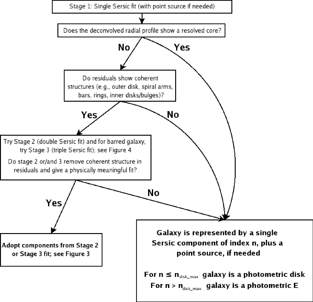
Figure 2: This figure provides an overview of our structural decomposition method. All galaxies are subjected to Stage 1, and most are further processed in Stage 2. A galaxy best fit with a single Sérsic profile plus point source (if needed) is interpreted as a photometric elliptical or photometric disk. A galaxy with extra coherent structure that cannot be described with a single Sérsic profile is subjected to a multiple-component fit in Stage 2 and, if needed, Stage 3. Figure 3 describes Stage 2 and Stage 3 in more detail.

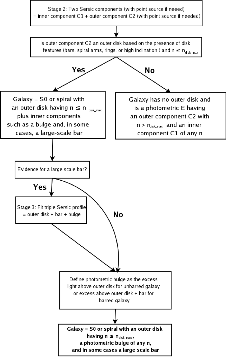
Figure 3: This figure shows the steps following stages 2 and 3 from Figure 2. A galaxy without an extended outer disk is interpreted as a photometric E, while a galaxy with such a disk is labeled either an S0 or spiral. When evidence for a large scale bar is found in a galaxy with an outer disk, Stage 3 is used to model the bar component.

Our structural decomposition scheme and decision sequence are described in detail in Appendix B, illustrated in Figures 2 and 3, and briefly outlined below:

• Stage 1 (Single Sérsic fit with nuclear point source if needed): The single Sérsic model is adopted if either the galaxy does not show any coherent structures (e.g., inner/outer disks, bars, bulges, rings, or spiral arms) indicating the need for additional Sérsic components, or, alternatively, if the galaxy has a core - a light profile that deviates downward from the inward extrapolation of the Sérsic profile (see Appendix C). Such galaxies are interpreted as photometric ellipticals if the single Sérsic index is above a threshold value $n_{\rm disk\_max}$ associated with disks (Section 3.1, Appendix B.2, and Appendix D); otherwise they are considered photometric disks. Three galaxies show convincing evidence for being cores, and these are luminous objects with high single Sérsic $n>n_{\rm disk\_max}$ (see Appendix B.2, Table 2, Appendix C). The results of Stage 1 are listed in Table 3. See Appendix B.1 for additional details on the single Sérsic fits.

• Stage 2 (Double Sérsic model with nuclear point source if needed): Galaxies showing coherent structure in the Stage 1 residuals are subjected to a two-component Sérsic + Sérsic fit, with nuclear point source if needed (see Figure 3). This two-component model is intended to model the inner (C1) and outer (C2) galaxy structures.

  There are two possible outcomes. a) If the outer component C2 is an outer disk based on having Sérsic index $n\leq n_{\rm disk\_max}$, then the galaxy is considered a spiral or S0 with an outer disk having a photometric bulge and, in some cases, a large-scale bar. b) If the outer component C2 does not meet our definition of an outer disk, then the galaxy is considered a photometric elliptical having an outer component C2 with $n>n_{\rm disk\_max}$ and an inner component C1 of any $n$. See Appendix B.2 for details.

• Stage 3 (Triple Sérsic model with nuclear point source if needed): Case (a) in Stage 2 identifies spiral and S0 galaxies with an outer disk. These galaxies are further processed as follows: a) If there is evidence for a large-scale bar (see Appendix B.2), then a triple Sérsic profile is fitted in Stage 3 for the photometric bulge, disk, and bar. b) Otherwise, the galaxy is considered as unbarred and the double Sérsic fit for a photometric bulge and disk is adopted. In both cases (a) and (b), it is important to note that the photometric bulge is allowed to have any Sérsic index $n$, thus allowing for structures with $n\leq n_{\rm disk\_max}$ and structures with $n>n_{\rm disk\_max}$.

3.3 Overview of Our Galaxy Classification Scheme

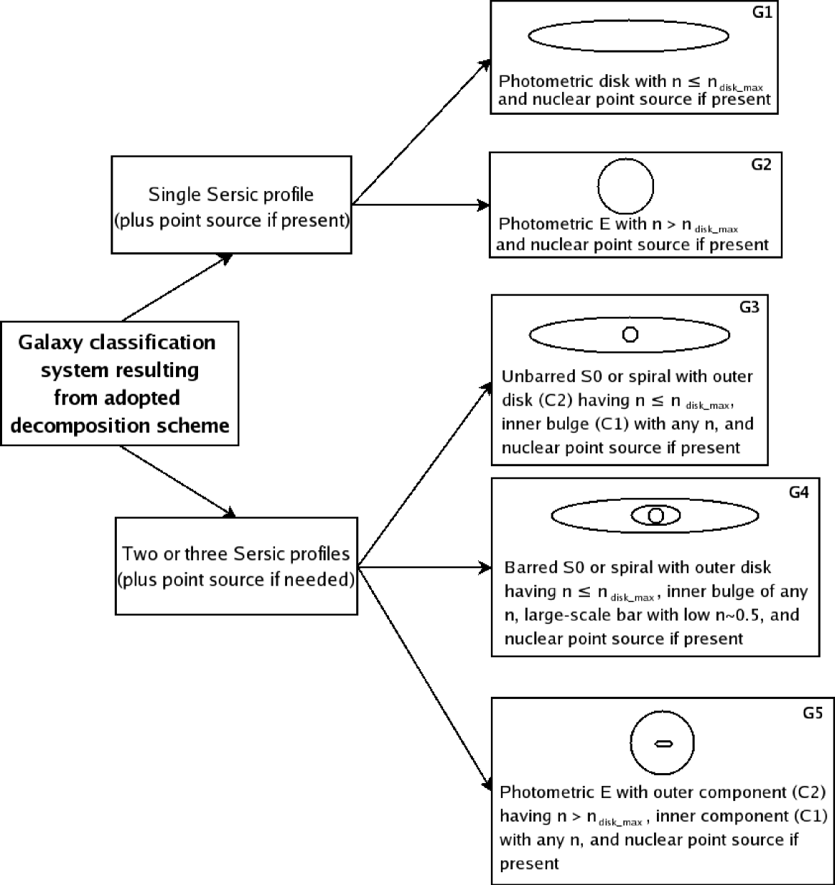
Figure 4: Overview of our galaxy classification system (Section 3.3). Galaxies are deemed to be best represented by a either a single or multi-component Sérsic profile (plus point source, if needed). Galaxies fitted with a single Sérsic profile are further interpreted as a pure disk (if Sérsic index $n\leq n_{\rm disk\_max}$) or photometric elliptical (if Sérsic index $n>n_{\rm disk\_max}$). When a multi-component Sérsic profile is required, the galaxy is either an unbarred/barred S0 or spiral, or a photometric E with inner and outer components. S0s and spirals must have an outer component C2 with Sérsic index $n\leq n_{\rm disk\_max}$. The inner component C1 can have any $n$. If the outer component C2 has Sérsic index $n>n_{\rm disk\_max}$, the galaxy is a photometric elliptical with inner component C1 of any $n$. The value of $n_{\rm disk\_max}$ is set to 1.66 based on several considerations (See Appendices B.2 and D). We determine $n_{\rm disk\_max}$ to be the maximum Sérsic index of the outer disk in spiral and S0 galaxies showing clear signs of an outer disk, such as bars, spiral arms, rings, or high inclination.

The decomposition scheme discussed above and in Figures 2 and 3 leads naturally to the galaxy classification system outlined in Figure 4, where there are five main galaxy types, G1 to G5. Systems best fitted by single Sérsic models (plus a nuclear point source if present) represent galaxies of type G1 and G2. Systems best fitted by two or three Sérsic profiles (plus a nuclear point source if present) represent galaxies of type G3 to G5.

1. G1: Photometric disk with $n\leq n_{\rm disk\_max}$ (plus a nuclear point source if present).

2. G2: Photometric elliptical with $n>n_{\rm disk\_max}$ (plus a nuclear point source if present).

3. G3: Unbarred S0 or spiral having an outer disk with $n\leq n_{\rm disk\_max}$ and an inner photometric bulge of any $n$ (plus a nuclear point source if present).

4. G4: Barred S0 or spiral having an outer disk with $n\leq n_{\rm disk\_max}$, a bar, and an inner photometric bulge of any $n$ (plus a nuclear point source if present).

5. G5: Photometric elliptical having an outer component with $n>n_{\rm disk\_max}$ and an inner component of any $n$.

This galaxy classification scheme has multiple advantages. Firstly, it allows us to identify low-$n$ disk-dominated structures within galaxies, both on large scales and in the central regions, in the form of outer disks with $n\leq n_{\rm disk\_max}$ in spirals and S0s, photometric bulges with $n\leq n_{\rm disk\_max}$ in spirals and S0s (representing disky pseudobulges), and inner disks within ellipticals represented by a component C1 having $n\leq n_{\rm disk\_max}$. Furthermore, it allows a census of galaxy components with $n>n_{\rm disk\_max}$ more akin to classical bulges/ellipticals. Our scheme does not allow for low-$n$ dynamically hot components. As discussed in Section 3.1, this is not a problem because in our sample such structures are not expected to be present in large numbers.

Table 4 lists the distribution of best-fit models for the sample of galaxies with stellar mass $M_{\star}\geq 10^{9}$ $M_{\odot}$, and the breakdown of galaxies into classes G1 to G5. Table 5 lists the structural parameters from the best single or multi-component model. In summary, we fit 6, 38, and 25 galaxies with 1, 2, and 3 Sérsic profiles, respectively. Our best-fit models have reduced $\chi^{2}$ of order one. In terms of galaxy types G1 to G5, we assign 1, 5, 24, 25, and 14 objects to classes G1, G2, G3, G4, and G5, respectively. The number of Stage 3 fits implies the bar fraction among galaxies with an extended outer disk is $50.0\pm 7.1\%$, and this is consistent with the bar fraction in Coma derived by Marinova et al. (2012).

4 Empirical Results on Galaxy Structure

4.1 Galaxy Types and Morphology-Density Relation in the Center of Coma

We next map classes G1 to G5 to more familiar Hubble types, namely cD, photometric E, S0, and spiral. The Hubble types assigned here depend only on the morphology classes (G1 to G5) associated with structural decomposition; they are independent of the morphological types from the Trentham et al. (in prep.) catalog discussed in Section 2. The results are shown in Table 4, and this process is explained in detail below.

The one object in class G1 (photometric disk) has a single Sérsic index $n\leq n_{\rm disk\_max}$ and a nuclear point source. This object has no visible spiral arms, so it is an S0. Objects assigned to class G2 (photometric ellipticals) have single Sérsic index $n>n_{\rm disk\_max}$ and include two known central cD galaxies, NGC 4874 and NGC 4889. We label these two sources separately as cD galaxies because they contain a disproportionately large fraction of the stellar mass. Classes G3 (unbarred S0, spiral) and G4 (barred S0, spiral) represent S0 or spiral disk galaxies with a possible large-scale bar. We label the six galaxies in either class G3 or G4 showing spiral arms in the data or residual images as spirals, while the remaining sources are labeled S0. Class G5 objects are identified as photometric ellipticals having an outer component with $n>n_{\rm disk\_max}$ and an inner component of any $n$.

Considering the Hubble types assigned above, we find evidence of a strong absence of spiral galaxies. In the projected central 0.5 Mpc of the Coma cluster, there are 2 cDs (NGC 4874 and NGC 4889), spirals are rare, and the morphology breakdown of (E+S0):spirals is (25.3%+65.7%):9.0% by numbers and (32.0%+62.2%):5.8% by stellar mass. Note that our ratio of E-to-S0 galaxies is lower than found elsewhere for Coma (e.g., Gavazzi et al. 2003) and for other clusters (e.g., Dressler 1980; Fasano et al. 2000; Poggianti et al. 2009), where it is $\sim 1-2$. This is driven by the effect of cosmic variance on our sample (Appendix B.5). Also, the total stellar mass cited here does not include the cDs as their stellar mass is quite uncertain (see Section 2.2).

In contrast to the central parts of Coma, lower-density environments are typically dominated by spirals. This is quantitatively illustrated by Table 6, which compares the results in Coma with the lower-density Virgo cluster and the field. We note that Virgo has significantly lower projected galaxy number densities and halo mass (Binggeli et al. 1987) than the center of Coma. McDonald et al. (2009) study a sample of 286 Virgo cluster member galaxies that is complete down to $B_{T}=16$ (Vega mag). At stellar mass $M_{\star}\geq 10^{9}$ $M_{\odot}$, if M87 is counted as a giant elliptical, the (E+S0):spirals breakdown is (34.1%+31.6%):34.8% by numbers and (59.2%+19.3%):21.4% by stellar mass. There is evidence (Mihos et al. 2005, 2009; Kormendy et al. 2009) that M87 has a cD halo, and after excluding M87, the (E+S0):spirals breakdown changes slightly to (33.5%+31.6%):34.8% by numbers and (57.2%+20.3%):22.5% by stellar mass. In the field, the (E+S0):spiral morphology breakdown is $\sim$ 20%:80% by number for bright galaxies (Dressler 1980).

4.2 What Fraction of Total Galactic Stellar Mass is in Disk-Dominated Structures Versus Classical Bulges/Ellipticals?

Here and in Section 4.3, we discuss the stellar mass breakdown among galaxy components within each galaxy type. Our results are summarized in Tables 7 and 8.

Recall that in Section 2.2, the total stellar masses were computed through applying calibrations of $M/L$ to the $HST$ F475W and F814W photometry. To calculate the stellar mass in galaxy substructures we assume a constant $M/L$ ratio and simply multiply the F814W light ratio of each component by the total galaxy stellar mass. A more rigorous approach is to also perform the decompositions in the F475W band and to fold the colors of galaxy substructures into the calculation. In Appendix B.6, we consider the effect of galaxy color gradients for a subset of galaxies; the effect of the color gradients on the stellar mass fractions is small ($\sim 5\%$) and does not impact our conclusions.

Table 7 summarizes our attempt at providing a census of the stellar mass among disk-dominated components and classical bulges/ellipticals, in the projected central 0.5 Mpc of Coma, excluding the two cDs. We highlight the main results below.

1. Stellar mass in low-$n$ flattened disk-dominated structures ($43\%$):
   The total stellar mass in small and large-scale disk-dominated components is $\sim 36.0\%$. Bars are disk-dominated components in the sense that they are flattened non-axisymmetric components. Bar proportions typically range from 2.5:1 to 5:1 in their equatorial plane (Binney & Tremaine 1987). The stellar mass percentage in bars is 6.8%. Thus, the total fraction mass in disk-dominated components is $43\%$.
   

2. Stellar mass in high-$n$ classical bulges/ellipticals ($57\%$):
   The remaining stellar mass is in components with $n>n_{\rm disk\_max}$. These components include the outer components of photometric ellipticals, the central components with $n>n_{\rm disk\_max}$ in photometric ellipticals, and the bulges of S0s and spirals with $n>n_{\rm disk\_max}$. The percent stellar mass in these systems is 57%.
   

3. Environmental dependence of disk-dominated structures :
   Finally, we discuss how $f_{\rm disk\_dominated}$, the fraction of galactic stellar mass in disk-dominated structures, varies with environment. For the lower density field-like environments studied by Weinzirl et al. (2009), this fraction $f_{\rm disk\_dominated}$ is $\sim 89.6\%$ for galaxies with $M_{\star}\geq 10^{10}$ $M_{\odot}$. Applying the same mass cut in Coma, the fraction $f_{\rm disk\_dominated}$ is $\sim 40.1\%$, which is lower than in the field as expected.

   Due to the effect of cosmic variance on our sample (Appendix B.5), our measurement of disk-dominated stellar mass is larger by an estimated factor of 1.27, compared to what would be obtained from an unbiased sample. This is estimated by weighting the fraction of hot and cold stellar mass in elliptical, S0, and spiral galaxies (Table 8) with the morphology-density distribution from GOLD Mine for the projected central 0.5 Mpc of Coma.

   We also note here the results for the Virgo cluster, in which Kormendy et al. (2009) find that in galaxies with $M_{\star}\gtrsim 5\times 10^{9}$ $M_{\odot}$, more than 2/3 of the stellar mass is in classical bulges/ellipticals, implying that $f_{\rm disk\_dominated}$ is less than 1/3. It may seem surprising that our value of $f_{\rm disk\_dominated}$ in Coma is higher than the value of 1/3 for Virgo. However, we believe this apparent discrepancy is due to the fact that the Virgo study includes the giant elliptical galaxy M87, which is marginally classified as a cD (Kormendy et al. 2009), while our study excludes the two cDs in the central part of Coma. If we include these 2 cDs and adopt a conservative lower limit for their stellar mass, then the fraction $f_{\rm disk\_dominated}$ of stellar mass in the low-$n$ component would be less than 27%, since the cDs add their mass to high-$n$ stellar components (see Appendix B.4).

4.3 What Fraction of Stellar Mass within S0, E, Spirals is in Disk-Dominated Structures versus Classical Bulges/Ellipticals?

We now discuss how the stellar mass is distributed among E, S0, and spiral Hubble types in the projected central 0.5 Mpc of Coma. As above, fractional stellar masses are reported without including the cD galaxies.

1. Mass distribution among high-$n$ classical bulges/ellipticals versus low-$n$ disky pseudobulges in Coma S0s and spirals:
   Bulges account for $\sim 30.5\%$ of the stellar mass across E, S0, and spiral galaxies. The ratio $R$ of stellar mass in high-$n$ ($n\gtrsim 1.7$) classical bulges to low-$n$ ($n\lesssim 1.7$) disky pseudobulges is $28.3\%/2.2\%$ or 12.9.
   

2. Mass distributions among bulges in Coma S0s versus S0s in lower-density environments:
   We next compare the bulges of Coma S0s versus S0s in lower-density environments (LDEs). The results are summarized in Table 9. We base this comparison on the results of Laurikainen et al. (2010), who derive structural parameters from $2D$ multi-component decompositions of 117 S0s in LDEs that include a mix of field and Virgo environments. For S0s in these LDEs with $M_{\star}\geq 7.5\times 10^{9}$ $M_{\odot}$, the ratio $R$ of stellar mass in high-$n$ ($n\gtrsim 1.7$) classical bulges to low-$n$ ($n\lesssim 1.7$) disky pseudobulges is 30.6%/4.7% or 6.5, while it is 41.7%/2.4% or 17.4 in the projected central 0.5 Mpc of Coma. Note the difference in mass stored in high-$n$ and low-$n$ bulges is not due to a greater frequency of high-$n$ bulges, which is similar at this mass range.
   

3. Mass distribution in outer and inner components of photometric ellipticals in Coma:
   By definition in Section 4.1, photometric ellipticals have no outer disk. The outer components of these ellipticals have Sérsic $n$ from 1.72 to 6.95, with a median value of 2.1. The total fractional stellar mass of the outer structures in ellipticals relative to our sample (minus the cDs) is $\sim 25.9\%$. Photometric ellipticals may contain an inner component of any Sérsic $n$, and we find a range in $n$ of 0.31 to 5.88 in Sérsic index, with a median of 1.0. Inner components with $n\leq n_{\rm disk\_max}$ represent compact inner disks analogous to the disky pseudobulges in S0s and spirals; most of these inner components (9/14 or $64.3\pm 12.8\%$) qualify as inner disks.

4.4 Scaling Relations for Outer Disks and Bulges

Here, we explore scaling relations for the bulges and outer disks in the projected central 0.5 Mpc of the Coma cluster. We assess how these structures compare with outer disks and bulges in LDEs, such as field, groups, and even low-density clusters similar to the Virgo cluster, where environmental processes and merger histories are likely to be different.

For this comparison, we use the results of Gadotti (2009), who studies face-on ($b/a\geq 0.9$) galaxies from the SDSS Data Release 2 in a volume limited sample at $0.02\leq z\leq 0.07$. He derives galaxy structure from 2D decompositions of multi-band $gri$ images that account for bulge, disk, and bar components. The Coma sample S0s/spirals have stellar mass $10^{9}\leq M_{\star}\leq 6\times 10^{10}$ $M_{\odot}$, and for this comparison we consider only galaxies with stellar mass $5\times 10^{9}\leq M_{\star}\leq 6\times 10^{10}$ $M_{\odot}$. We proceed with the caveat that the sample from Gadotti (2009) is incomplete in mass for $M_{\star}\lesssim 5\times 10^{10}$ $M_{\odot}$.

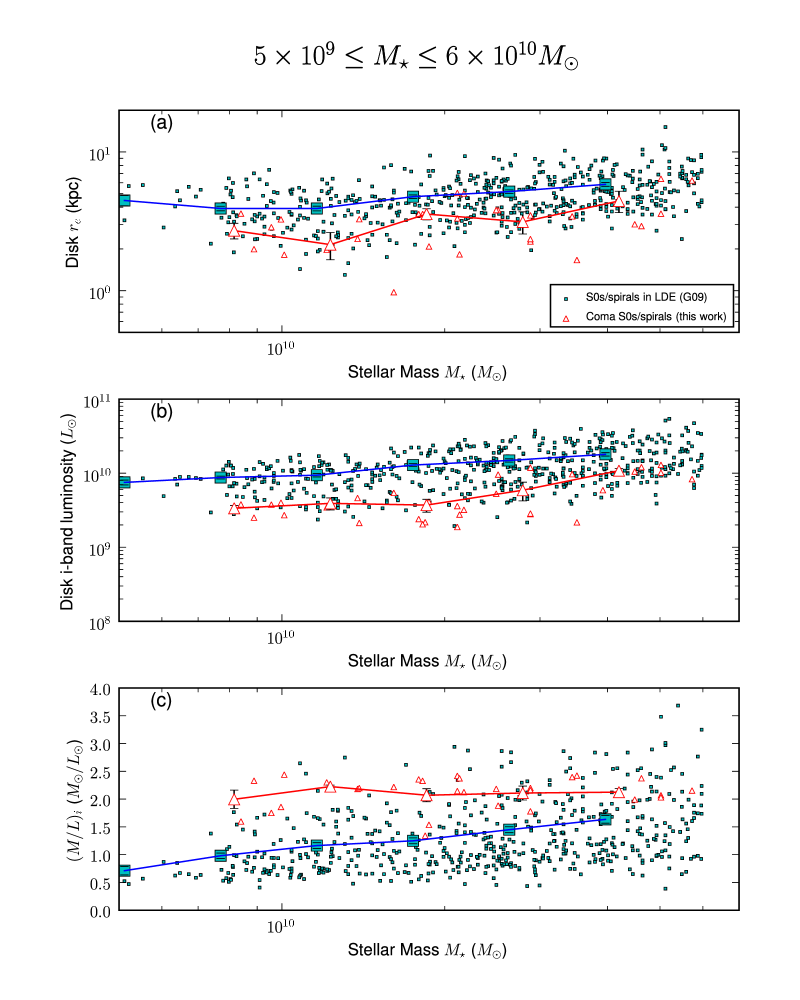
Figure 5: Panels (a) and (b) compare the properties of large-scale disks ($r_{\mathrm{e}}$, luminosity) with galaxy stellar mass $M_{\star}$. Massive ($5\times 10^{9}\leq M_{\star}\leq 6\times 10^{10}$ $M_{\odot}$) S0/spiral galaxies from the projected central 0.5 Mpc of Coma as well as low-density environments (LDEs) are considered. The LDE sample is from Gadotti (2009) and includes galaxies in SDSS Data Release 2 that are face-on ($b/a\geq 0.9$) and have redshift $0.02\leq z\leq 0.07$. In panel (b), the $i$-band luminosity represents the ACS F814W photometry for Coma galaxies and the SDSS $i$-band photometry for the LDE galaxies. Panel (c) compares $i$-band mass-to-light ratio $(M/L)_{i}$ with galaxy $M_{\star}$. For Coma, the galaxy wide mass-to-light ratio is plotted, while for LDEs the outer disk $(M/L)_{i}$ is shown. In all panels, the mean values (large symbols) in galaxy $M_{\star}$ for Coma and LDEs are slightly offset along the x-axis, as shown by the red triangle and blue squares, in order to avoid the error bars from overlapping. The mean values are calculated in 0.18 dex bins. The error bars on the mean values represent the standard error on the mean. This figure demonstrates that at a given galaxy stellar mass, the average disk half-light radius $r_{\mathrm{e}}$ in the $i$-band is smaller in the projected central 0.5 Mpc of Coma compared to LDEs.

Figure 5 compares properties of large-scale disks (size, luminosity) with galaxy $M_{\star}$. Figure 5a explores the projected half-light radius in the $i$-band ($r_{\mathrm{e}}$) of outer disks along the major axis at a given galaxy $M_{\star}$ in Coma versus LDEs. It shows that at a given galaxy $M_{\star}$, the average disk $r_{\mathrm{e}}$ is smaller in the projected central 0.5 Mpc of Coma compared with LDEs by $\sim 30-82\%$. While the scatter in disk $r_{\mathrm{e}}$ is large, the separation between the two mean values in each mass bin is larger than the sum of the errors. The suggestion that outer disks in Coma are more compact is consistent with the results of previous analyses of disk structure in Coma (Gutiérrez et al. 2004; Aguerri et al. 2004). Figure 5b makes a similar comparison for the outer disk luminosity between Coma and LDEs. We use here the ACS F814W photometry for Coma and the SDSS $i$-band photometry from Gadotti (2009). At a given stellar mass, the average outer disk luminosities are fainter by $\sim 40-70\%$, excluding the lowest mass bin.

We next consider the effect of $M/L$ to test if the difference in outer disk luminosity could imply a a difference in outer disk mass. For Coma, we show the galaxy-wide $(M/L)_{i}$ ratio estimated, while for the Gadotti (2009) sample we show $i$-band $M/L$ ratios in the outer disks, $(M/L)_{d,i}$. Figure 5c compares the resulting $(M/L)$ values against galaxy $M_{\star}$. The average $(M/L)_{i}$ in Coma is larger than the average $(M/L)_{d,i}$ in LDEs by a factor of $\sim 1.3-2$ at a given galaxy $M_{\star}$, excluding the lowest mass bin. This difference in $(M/L)_{i}$ accounts for $\sim 48-80\%$ of the average offset in disk luminosity. This suggests some of the difference in outer disk luminosity might be driven by a real difference in outer disk mass. Cappellari (2013), in comparison, concludes that spirals in Coma transformed into fast rotating early-type galaxies while decreasing in global half-light radius with little mass variation.

Figure 6 examines how bulge size ($r_{\mathrm{e}}$), bulge luminosity, bulge Sérsic index, and bulge-to-disk light ratio ($B/D$) scale with galaxy $M_{\star}$. Figures 6a-c show that bulge size, bulge luminosity, and bulge Sérsic index as a function of galaxy $M_{\star}$ are not systematically offset in Coma versus LDEs. Figure 6d shows there is a great scatter in $B/D$ versus galaxy $M_{\star}$.

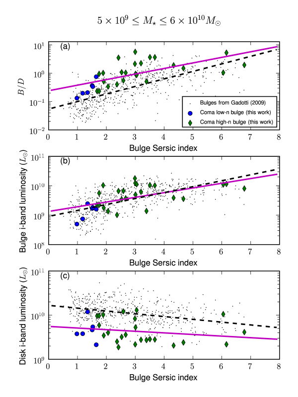
Figure 7: This figure shows a comparison of bulges in massive ($5\times 10^{9}\leq M_{\star}\leq 6\times 10^{10}$ $M_{\odot}$) S0/spiral galaxies in low-density environments (LDEs) from Gadotti (2009) versus galaxies in the projected central 0.5 Mpc of Coma. See Section 4.4 and Figure 5 for extra details on the sample from Gadotti (2009). Bulges in Coma are divided into groups of low Sérsic index ($n\leq n_{\rm disk\_max}$) and high Sérsic index ($n>n_{\rm disk\_max}$). Panel (a) shows bulge-to-disk light ratio ($B/D$) versus bulge Sérsic index. Panels (b) and (c) show bulge and disk $i$-band luminosity, respectively, versus bulge Sérsic index. In each panel, the solid line represents the fit to Coma bulges of all Sérsic $n$, and the dashed line is the corresponding fit to bulges of all Sérsic $n$ from LDEs. The offset in $B/D$ in panel (a) appears to be driven, at least in part, by the offset in disk luminosity in panel (c).

Figure 7a shows $B/D$ versus bulge Sérsic index. At a given bulge Sérsic index, galaxies in Coma show a systematically higher average $B/D$ ratio than galaxies in LDEs. A linear regression fit reveals a clear offset in $B/D$ for a given bulge index. Figure 7b indicates that at a given bulge Sérsic index the bulge luminosities in Coma and LDEs are very consistent. Figure 7c, on the other hand, shows a clear offset in disk luminosity ($\sim 0.6$ mag), indicating that differences in $B/D$ are due, at least in part, to outer disk size/luminosity.

From this investigation, we have learned of a reduction in the average sizes and luminosities in the outer disks of Coma galaxies that may translate into a lower mean outer disk stellar mass. This may be explained in part by cluster environmental effects. We consider this point further in Section 4.5.

4.5 Environmental Processes in Coma

Many studies provide evidence for the action of environmental processes in Coma. The predominantly intermediate or old stellar populations in the center of the cluster (e.g., Poggianti et al. 2001; Trager et al. 2008; Edwards & Fadda 2011) are indirect evidence for the action of starvation. Furthermore, the properties of Coma S0s display radial cluster trends that favor formation processes that are environment-mediated (Rawle et al. 2013, Head et al. 2014). Several examples of ram-pressure stripping have been directly observed in Coma (Yagi et al. 2007, 2010; Yoshida et al. 2008; Smith et al. 2010; Fossati et al. 2012). There is also much evidence for the violent effects of tidal forces. The presence of a diffuse intra-cluster medium around Coma central galaxies NGC 4874 and NGC 4889 has long been discussed (Kormendy & Bahcall 1974; Melnick et al. 1977; Thuan & Kormendy 1977; Bernstein et al. 1995; Adami et al. 2005; Arnaboldi 2011). At the cluster center, the intra-cluster light represents up to $20\%$ of the cluster galaxy luminosity (Adami et al. 2005). This central intra-cluster light is not uniform given the presence of plumes and tidal tails (Gregg & West 1998; Adami et al. 2005), and debris fields are also found further outside the cluster center (Gregg & West 1998; Trentham & Mobasher 1998).

Below, we comment on how our results add to this picture.

1. Reduced Growth and Truncations of Outer Disks in Coma S0s/spirals:
   In Section 4.4, we found that at a given galaxy stellar mass, the average half-light radius ($r_{\mathrm{e}}$) of the outer disk in S0s/spirals is $\sim 30-82\%$ smaller, and the average disk $i$-band luminosity is $\sim 40-70\%$ fainter in Coma than in lower-density environments (Figure 5). These observations may be explained in part by cluster environmental effects (e,g., strangulation, ram-pressure stripping, tidal stripping) that suppress the growth of large-scale disks. Hot gas stripping (strangulation) can plausibly suppress disk growth by limiting the amount of gas that can cool and become part of the outer disk. Tidal stripping via galaxy harassment is predicted (e.g., Moore et al. 1999) to be particularly efficient at removing mass from extended disks. Ram-pressure stripping is most effective at removing HI gas in the outskirts of a large scale-disk. The evidence (Yagi et al. 2007, 2010; Yoshida et al. 2008; Fossati et al. 2012) suggests ram-pressure stripping happens quickly, and if so it should be effective at preventing the growth of large-scale disks after the host galaxy enters the cluster.
   

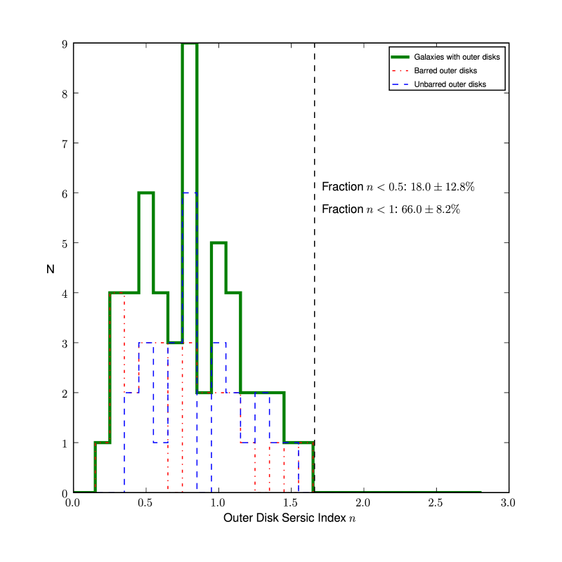
Figure 8: The distribution of Sérsic index for outer disks in S0/spiral galaxies. The vertical line represents the empirically determined upper limit, $n_{\rm disk\_max}$, in the Sérsic index of outer barred disks, which can be considered unambiguous cases of outer disks due to the presence of a bar. The dash-dotted and dashed lines show the distributions for barred and unbarred outer disks, respectively. See Section 3.3 and Appendix B.2 for details.

2. Low Sérsic index in S0/spiral outer disks:
   Figure 8 demonstrates the majority of outer disks have low Sérsic index ($66.0\pm 8.2\%$ with $n<1$ and $18.0\pm 12.8\%$ with $n<0.5$). This effect is not artificially driven by bars because the low $n<1$ disks include barred and unbarred galaxies to similar proportions, and additionally, the disks are fitted separately from the bars in our work. Similar examples have been found in Virgo. Kormendy & Bender (2012) find several examples of Gaussian ($n\sim 0.5$) disks among both barred and unbarred galaxies, which commonly occur in barred galaxies (e.g., Kormendy & Kennicutt 2004). Gaussian-like disks among unbarred galaxies are much more surprising (Kormendy & Bender 2012). Figure 8 shows that the large fraction of $n<1$ outer disks in Coma is not driven by barred galaxies alone. It is not easy to compare the fraction of low $n<1$ disks in Coma versus LDEs because most work to date in LDEs (e.g., Allen et al. 2006; Laurikainen 2007, 2010; Weinzirl et al. 2009) fit the outer disk with a fixed $n=1$ exponential profile.

   Environmental processes could be creating the Gaussian-like disks. Kormendy & Bender (2012) have suggested this and invoked dynamical heating. We could be seeing a stronger and/or different manifestation in Coma. Ram-pressure stripping and tidal stripping can plausibly reduce the Sérsic $n$ by cutting off the outskirts of the outer stellar/gaseous disk.
   

3. Bulge-to-disk ratio ($B/D$):
   The mean bulge Sérsic index rises with mean $B/D$ light ratio in both the central part of Coma and LDEs, consistent with the idea that the development of high $B/D$ ratio in galaxies is usually associated with processes, such as major mergers, which naturally results in a high $n$. Such a correlation was also found previously in field spirals (e.g., Andredakis et al. 1995; Weinzirl et al. 2009).

   We also find that at a given bulge index, the $B/D$ light ratio is higher for Coma. This environmental effect appears to be due, at least in part, to the fact that at a given bulge $n$, the bulge luminosity is similar in Coma and LDEs, but the outer disks have lower luminosity by a factor of a few in Coma (Figure 7). This reduced disk growth is likely due to cluster environmental effects suppressing the growth of large-scale outer disks. This conclusion for Coma nicely parallel studies of ram-pressure stripping (Cayette et al. 1990, 1994; Kenney et al. 2004, 2008; Chung et al. 2007, 2009) and dynamical heating (Kormendy & Bender 2012) in the less extreme Virgo cluster.

5 Comparison of Empirical Results With Theoretical Predictions

5.1 Overview of the Models

In this section, we compare our empirical results for Coma with simulations of clusters. The simulated clusters are derived from a semi-analytical model (SAM) based on Neistein & Weinmann (2010). The SAM is able to produce reasonable matches (Wang, Weinmann, & Neistein 2012) to the galaxy stellar mass function determined by (Li & White 2009) for massive $M_{\star}\gtrsim 5\times 10^{8}$ $M_{\odot}$ galaxies at low redshift ($0.001<z<0.5$) over all environments (including Virgo and Coma) probed in the northern hemisphere component of SDSS Data Release 7. A brief summary of the SAM formalism is given below. Interested readers should see Neistein & Weinmann (2010) and Wang, Weinmann, & Neistein (2012) for additional details.

The SAM uses merger trees extracted from the Millennium $N$-body simulation (Springel et al. 2005). Galaxies are modeled as vectors of stellar mass, cold gas, and hot gas. Baryonic physics are handled with semi-analytic prescriptions. In between merger events, the efficiencies of quiescent evolutionary processes, such as cold and hot gas accretion, gas cooling, star formation, and supernovae feedback, are modeled as functions of halo mass and redshift only. The star formation rate is proportional to the amount of cold gas, and the star formation efficiency is a function of halo mass and redshift. In the model, the baryonic mass (i.e., the sum of stellar and cold gas mass) is used to define major ($M_{1}/M_{2}\geq 1/4$) and minor ($1/10<M_{1}/M_{2}<1/4$) mergers. As we will discuss in Section 5.4, the results are highly sensitive to whether the stellar mass ratio or baryonic mass ratio are used.

Immediately after a major merger, the remnant’s stellar $B/T$ ratio is always one. This is because the model assumes any existing stellar disks are destroyed, and all stars undergo violent relaxation to form a bulge/elliptical. After a major merger, an extended stellar disk is rebuilt via gas cooling, causing $B/T$ to fall. Any further major mergers will reset $B/T$ to one. During a minor merger, the stellar component of the satellite of baryonic mass $M_{1}$ is added to the bulge.

During a major/minor merger, some fraction of cold gas is converted to stars in a short induced starburst $\sim 10$ Myr in duration. The amount of merger-induced star formation depends explicitly on the cold gas mass. Stars formed in major merger-induced starbursts are considered part of the bulge (see Section 5.6). This is a reasonable assumption given that a) the bursts of star formation are much shorter than the overall duration of the mergers and b) all existing stars from both progenitors are violently relaxed during final coalescence. It seems less likely the starburst stars induced in minor mergers should be violently relaxed since minor mergers are not very efficient at violently relaxing stars in the host galaxy. We consider this issue further in Section 5.6. Therefore, in the model used in this paper, the bulge stellar mass traces the mass assembled via major and minor mergers. Galaxies without bulges have had no resolvable merger history. The model does not build bulges through the coalescence of clumps condensing in violent disk instabilities (Bournaud, Elmegreen, & Elmegreen 2007; Elmegreen et al. 2009).

Galaxy clusters impose additional environmental effects that complicate modeling with SAMs. The SAM used here accounts for stripping of hot gas (i.e., strangulation; Larson et al. 1980) by assuming hot gas is stripped exponentially with a timescale of 4 Gyr. Other processes like ram-pressure, stripping/disruption of stellar mass (Moore et al. 1996, 1998, 1999; Gnedin 2003), dynamical friction heating by satellite (El-Zant et al. 2004), and gravitational heating by infalling substructures (Khochfar & Ostriker 2008) are neglected. It is not clear how much the inclusion of ram-pressure stripping in the SAM would affect our results. While hydrodynamical simulations clearly demonstrate the strong influence of ram-pressure stripping on gas mass, galaxy morphology, and star formation (e.g., Quilis et al. 2000; Tonnesen & Bryan 2008, 2009, 2010), some SAMs (e.g., Okamoto & Nagashima 2003; Lanzoni et al. 2005) suggest that accounting for ram-pressure stripping has only a small affect. Tidal stripping creates a population of intra-cluster stars that can contribute between $10-40\%$ of the optical light in rich clusters (e.g., Bernstein et al. 1995; Feldmeier et al. 2004; Zibetti et al. 2005). The inclusion of tidal stripping in SAMs is important for addressing a wide range of systematic effects (e.g., Bullock et al. 2001; Weinmann et al. 2006; Henriques et al. 2008, 2010), but tidal stripping is not present in this SAM.

5.2 The Mass Function and Cumulative Number Density in Coma

In order to compare galaxies in the simulations with those in the center of Coma, we first need to identify model clusters that best represent Coma. We do this based on the global properties of Coma, namely the halo mass and size, galaxy stellar mass function, and radial profile of cumulative projected galaxy number density. As the ACS coverage of Coma encompasses a fraction (19.7%) of the projected central 0.5 Mpc, we calculate these properties in Coma with Data Release 7 (DR7) of the NYU Value-Added Galaxy Catalog (NYU-VAGC, Blanton et al. 2005), which provides full spatial coverage of Coma. NYU-VAGC DR7 is based on SDSS DR7 data (Abazajian et al. 2009) and provides catalogs generated from an independent, and improved, reduction of the public data (Padmanabhan et al. 2008).

We select Coma cluster member galaxies from NYU-VAGC assuming Coma cluster galaxies have radial velocity in the range v_min = 4620 km/s to v_max = 10,000 km/s, which is the range in radial velocity among spectroscopically confirmed members in the ACS survey. We also adopt the Coma virial radius and virial mass to be 2.9$h^{-1}_{70}$ Mpc and $1.4\times 10^{15}h^{-1}_{70}$ $M_{\odot}$, respectively, measured by Lokas & Mamon (2003) with a 30% accuracy, where $h^{-1}_{70}=H_{0}/70$. For our adopted $H_{0}$ of 73, we scale these numbers by $(73/70)^{-1}$, so that the virial radius and virial mass are 2.8$h^{-1}_{73}$ Mpc and $1.3\times 10^{15}h^{-1}_{73}$ $M_{\odot}$, respectively. We select galaxies with the following criteria:

1. Radial velocity in range 4620 to 10,000 km/s.

2. Projected radius, ${\rm{R_{p}}}$ from the cluster center (i.e., NGC 4874) less than the virial radius.

3. Brightness exceeding the SDSS spectroscopic completeness limit of $r=17.7$ mag, or $M_{r}\leq-17.3$ mag at the 100 Mpc distance of Coma. This corresponds to a stellar mass of $1.3\times 10^{9}$ $M_{\odot}$ assuming a $g-r$ color of 0.67, which is the average among Coma galaxies in the NYU-VAGC selected in this manner.

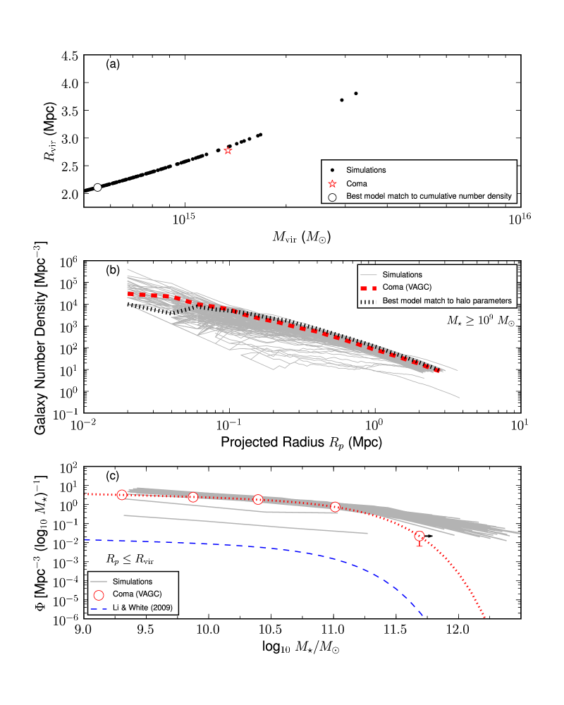
Figure 9: This figure shows how the global parameters of the Coma cluster compare with all 160 clusters in the Millennium simulation having a halo mass in the range $5\times 10^{14}-10^{16}$ $M_{\odot}$. The solid lines and black data points represent the simulated clusters. In panel (a), the virial mass and virial radius adopted for Coma are 2.8$h^{-1}_{73}$ Mpc and $1.3\times 10^{15}h^{-1}_{73}$ $M_{\odot}$ (Section 5.2). The open circle is the model cluster having the best match to the projected galaxy number density of Coma. In panels (b) and (c), the cumulative projected galaxy number density and the galaxy mass stellar function of Coma at projected radius $R_{\rm p}\leq R_{\rm vir}$ are based on data from the NYU Value-Added Galaxy Catalog (NYU-VAGC, Blanton et al. 2005). In panel (b), the dotted line represents the cumulative galaxy number density of the model cluster best matching the Coma halo parameters. In panel (c), for the Coma galaxy stellar mass function, we measure a slope $\alpha=-1.16$ and characteristic mass $M^{*}=1.17\times 10^{11}~{}M_{\odot}$. The last mass bin in the global mass function for Coma contains the two cD galaxies, and the arrow on this bin indicates the adopted stellar masses for the cDs are lower limits. The simulations are based on a model that produces a reasonable match to the galaxy stellar mass function of Li & White (2009) averaged over all environments at $0.001<z<0.5$ (dashed line). However, they cannot produce a model cluster that simultaneously matches multiple global properties (halo properties, galaxy number density, and galaxy stellar mass function), of Coma, our local benchmark for one of the richest nearby galaxy clusters.

Panel (b) of Figure 9 shows the resulting projected galaxy density profile for this set of Coma galaxies.

We next calculate the global galaxy stellar mass function within the virial radius. Figure 9c shows the result. This mass function includes normal massive galaxies (E, S0, spiral) as well as the two cDs (NGC 4874 and NGC 4889). As described in Section 2.2, we derive the stellar mass by applying Equations 5 and 6 to SDSS $gr$ photometry.

Using the cD galaxy stellar masses as lower limits at the high mass end of the galaxy stellar mass function in Figure 9c, we measure a slope $\alpha=-1.16$ and characteristic mass $M^{*}=1.25\times 10^{11}~{}M_{\odot}$ for the global galaxy stellar mass function of Coma inside the cluster virial radius.

5.3 Global Properties of Model Clusters Versus Coma

Next, we compare the above global properties of the Coma cluster with the simulated clusters in the theoretical model in order to identify the model clusters that best represent Coma. We consider all 160 Friend-of-Friend (FOF, Davis et al. 1985) groups in the Millennium simulation having a halo mass in the range $5\times 10^{14}-10^{16}$ $M_{\odot}$. We refer to the most massive halo, and its gravitationally bound subhaloes, in each FOF group as a ‘cluster’.

To find potential matching clusters, we identify massive ($M_{\star}\geq 10^{9}$ $M_{\odot}$) member galaxies in each cluster in a way that is consistent with the selection of Coma member galaxies in Section 5.2:

1. Radial velocity matching the range in line-of-sight velocities in the xy, xz, yz projections of the cluster.

2. Projected radius, ${\rm{R_{p}}}$, from the cluster center less than the cluster virial radius.

3. Luminosity brighter than the SDSS spectroscopic completeness limit of $M_{r}\leq-17.3$ mag at the 100 Mpc distance of Coma.

To gauge how well the simulated clusters compare with Coma in terms of global properties, we examine the match in cumulative number density, mass function, and halo parameters (virial mass and radius).

In Figure 9, we gauge how the global properties of Coma compare with those of all 160 cluster simulations. Figure 9a shows the combinations of virial radius and halo masses of the simulated clusters. The Coma halo parameters (virial mass and radius) adopted in Section 5.2 are well matched to the largest and most massive model clusters.

Figure 9b shows the radial profile of cumulative galaxy number density. The central galaxy number densities in the simulated clusters span three orders of magnitude from $\sim 10^{4}$ to $\sim 4\times 10^{5}$ Mpc^-3, overlapping with the high central density in Coma ($\sim 3\times 10^{4}$ Mpc^-3). The thick dotted line denotes the cluster model with the best-matching halo parameters from Figure 9a. This halo model does a good job at matching the galaxy number density profile of Coma at projected radius $R_{p}>0.7$ Mpc, but not at smaller projected radii. In comparison, the model with the best matching cumulative number density profile, shown as the open circle in Figure 9a, is smaller by $\sim 60\%$ in halo mass than Coma. The next nine best matches to cumulative number density also differ in halo mass by $\sim 30\%$ or more from the halo mass in Coma, which is estimated to be accurate to within 30% (Section 5.2).

Figure 9c compares the galaxy stellar mass function between Coma and the simulated model clusters. All the model clusters produce too many extremely massive ($M_{\star}\gtrsim 5\times 10^{11}$ $M_{\odot}$) galaxies. These very high-mass galaxies are not devoid of ongoing star formation like ellipticals in Coma are (Section 4.5). Rather, these galaxies have present day SFR of $\sim 10$ $M_{\odot}$ yr^-1. Furthermore, the cluster mass functions show slopes that are marginally too steep ($\alpha\sim-1.5$ versus $\alpha=-1.16$) on the low-mass end (Section 5.2).

We note that when this SAM model was compared with SDSS observations of galaxies averaged over all environments at low redshift (Wang, Weinmann, & Neistein 2012), the model galaxy stellar mass function shows a similar, but less extreme, discrepancy with the galaxy stellar mass function of Li & White (2009) in terms of producing too many of the most massive galaxies. Figure 9c includes the galaxy stellar mass function from Li & White (2009) as a dashed line for comparison.

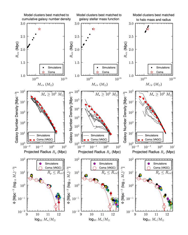
Figure 10: This figure shows the three sets of simulated model clusters (30 model clusters in total) chosen to best match, separately, the cumulative galaxy number density (Column 1), the galaxy stellar mass function (Column 2), and halo parameters (halo mass and virial radius, Column 3). The solid lines and solid circles in each panel represent the different simulated clusters. Rows 1, 2, and 3 show how the different simulated clusters compare with the global properties (halo mass and radius, cumulative galaxy number density, and galaxy stellar mass function) determined with data from the NYU Value-Added Galaxy Catalog (NYU-VAGC, Blanton et al. 2005) for Coma in Section 5.2. No model cluster simultaneously matches all three global properties.

In Figure 10 we make the comparison with three sets of model clusters (a total of 30 model clusters) containing the 10 best matches to Coma in terms of the cumulative galaxy number density, galaxy stellar mass function, and halo parameters. Matching to one criterion (e.g., cumulative number density) does not ensure a good match to the other two criteria.

We are left with the sobering conclusion that the simulations cannot produce a model cluster simultaneously matching multiple global properties of Coma, our local benchmark for one of the richest nearby galaxy clusters. The large discrepancy in the galaxy stellar mass function between the model and Coma could be due to a number of factors. The model currently does not include tidal stripping/disruption of stars and ram-pressure stripping (Section 5.1), which would reduce the stellar mass of galaxies on all mass scales. The importance of ram pressure stripping is further discussed in Section 5.5, where we find that the cold gas fraction in the model galaxies is much higher in Coma galaxies.

5.4 Strong Dependence of Results on Mass Ratio Used to Define Mergers

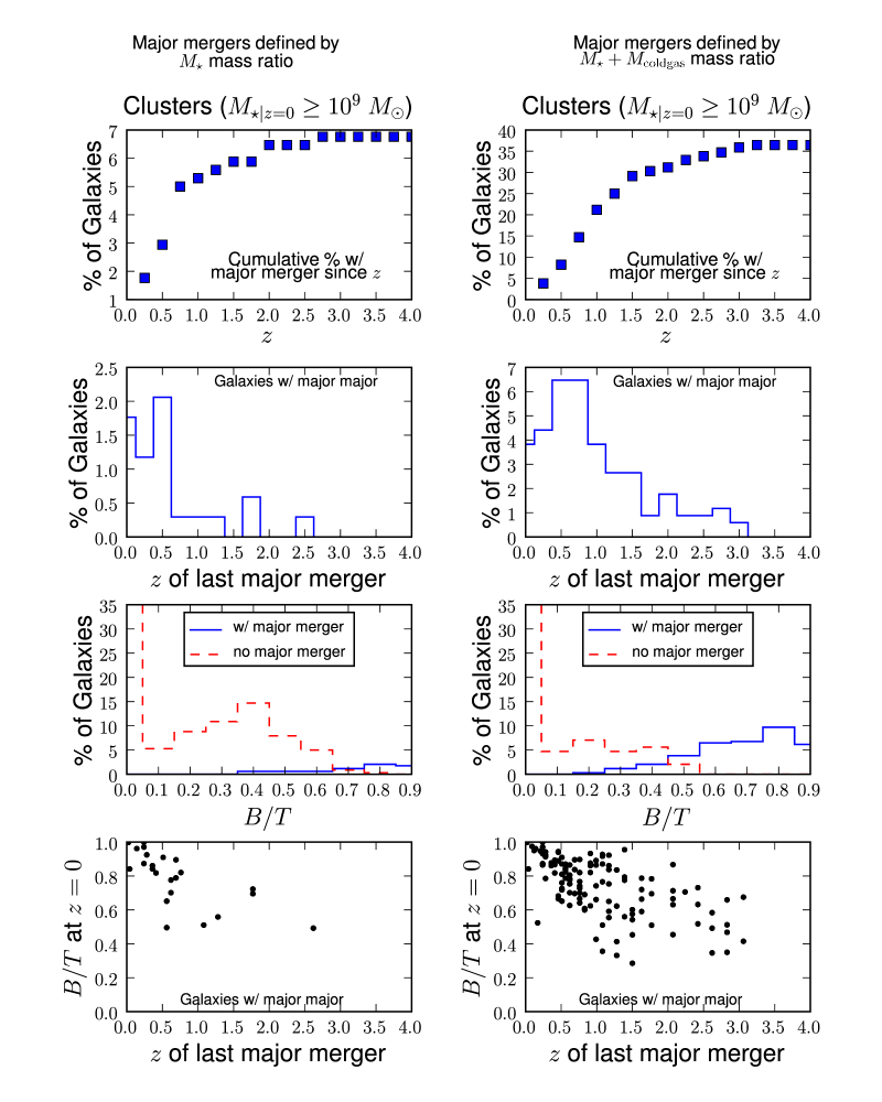
Figure 11: This figure highlights the effect that the definition of the merger mass ratio $M_{1}/M_{2}$ has on certain galaxy properties (merger history and $B/T$), for a representative model cluster (see Section 5.4). Note we require a major merger to have $M_{1}/M_{2}\geq 1/4$. The left column is the manifestation of the model cluster when $M_{1}/M_{2}$ refers to the stellar mass ratio, and in the right column the merger mass ratio represents cold gas plus stars. The two mass ratio definitions lead to vastly different merger histories and significantly affect the resulting distribution of $B/T$.

Merger history and galaxy $B/T$ are highly dependent on the mass used (stellar mass, baryonic mass, halo mass) to define merger mass ratio $M_{1}/M_{2}$. For a single representative cluster model, Figure 11 highlights the key differences that arise when $M_{1}/M_{2}$ is defined as the ratio of stellar mass (Def 1, left column) versus cold gas plus stars (Def 2, right column). This representative cluster was selected because it is the best matching cluster to the cumulative galaxy number density distribution in Coma (Figure 10). The first row of Figure 11 shows the cumulative percentage of galaxies with a major merger since redshift $z$. In the second row of Figure 11, the histograms show the percentage of galaxies with a last major merger at redshift $z$. The third row shows the percentage of galaxies with a given $B/T$ value, sorted by galaxies with and without a major merger. Finally, the last row of Figure 11 gives the distribution of present-day $B/T$ versus redshift of the last major merger.

In the following sections, we consider a model where the merger mass ratio $M_{1}/M_{2}$ depends on stellar mass plus cold gas, as this ratio is understood to be the most appropriate definition (Hopkins et al. 2009b). Traditionally, observers have tended to use stellar mass ratios in identifying mergers (e.g., Lin et al. 2004; Bell et al. 2006; Jogee et al. 2009; Robaina et al. 2010) as stellar masses are readily measured for a large number of galaxies. However, with the advent of ALMA, it will be increasingly possible to incorporate the cold gas mass for a large number of galaxies.

5.5 Cold Gas Mass in Coma Galaxies Versus Model Galaxies

In the SAM used here, the cold gas fraction $f_{\rm gas}$ (defined as the ratio of cold gas to the baryonic mass made of cold gas, hot gas, and stars) and the ratio ($M_{\rm cold\_gas}/M_{\star}$) of cold gas to stellar mass are both overly high. The issue of high cold gas fraction in this model was highlighted and discussed in Wang, Weinmann, & Neistein (2012). Here, we quantify how far off the model values are compared with what is expected for a rich cluster like Coma.

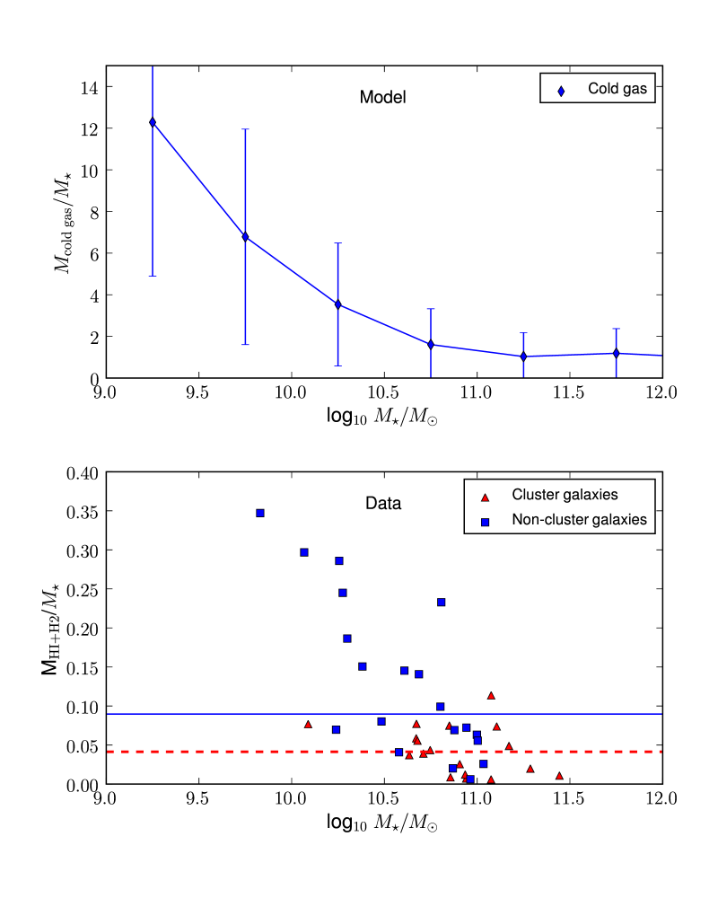
Figure 12: The top panel shows the ratio of cold gas to stellar mass ($M_{\rm cold\_gas}/M_{\star}$) for the best cluster model matched by cumulative galaxy number density (see Figure 10, column 1). The error bars represent the $1\sigma$ standard deviation around the mean value. The bottom panel shows the ratio of observed cold gas ($HI+H_{2}$) to stellar mass ($M_{HI+H_{2}}/M_{\star}$) for galaxies studied by Boselli et al. (1997) that are part of or near the Coma cluster. The dashed line is the median ratio (0.04) for Coma cluster galaxies, and the solid line is the median ratio (0.09) for the non-cluster galaxies. At $10^{10}\lesssim M_{\star}\lesssim 10^{11}$ $M_{\odot}$, the model predicts a cold gas to stellar mass ratio that is a factor $\sim 25-87$ times higher than the median value observed in Coma cluster galaxies.

Figure 12 illustrates the degree to which the ratio ($M_{\rm cold\_gas}/M_{\star}$) is overestimated by comparing with data from Boselli et al. (1997), who measure atomic ($M_{HI}$) and molecular gas ($M_{H_{2}}$) masses for Coma cluster member galaxies and non-cluster galaxies. The top panel shows that the average ratio of cold gas to stellar mass ($M_{\rm cold\_gas}/M_{\star}$) ranges from $\sim 1-12$ for a representative model cluster. The bottom panel shows that the ratio of $M_{HI+H_{2}}/M_{\star}$ for Coma cluster galaxies from Boselli et al. (1997) is usually $<0.1$; non-cluster galaxies are more gas rich, but the ratio of $M_{HI+H_{2}}/M_{\star}$ is still $\ll 1$. At $10^{10}\lesssim M_{\star}\lesssim 10^{11}$ $M_{\odot}$, the model predicts a cold gas to stellar mass ratio that is a factor $\sim 25-87$ times higher than the median in Coma cluster galaxies.

5.6 Data Versus Model Predictions for Stellar Mass in Dynamically Hot and Cold Components

We next proceed to compare the observed versus model predictions for the distribution of mass in dynamically hot and cold stellar components. The following comparisons are made in the projected central 0.5 Mpc of Coma and the model clusters.

We first start by describing how the model builds bulges and ellipticals. In the model, the total bulge stellar mass $M_{\rm\star,Bulge,model}$ consists of stellar mass accreted in major and minor mergers, plus stellar mass from SF induced in both types of mergers.

Next, we discuss how to compare the model with the data. For our sample of Coma galaxies (excluding the 2 cD systems) with $M_{\star}\geq 10^{9}$ $M_{\odot}$, we compute the ratio R1_data as the the stellar mass in all components with $n>n_{\rm disk\_max}$ to the sum of galaxy stellar mass. The reasons for not including the cD systems were discussed in Section 2.2. From Section 4.2, R1_data is 57%.

We next compare this ratio to the corresponding quantity in the model. The comparison is not entirely straightforward as the model does not give a Sérsic index. We therefore have to associate components in the model to the corresponding high $n>n_{\rm disk\_max}$ classical bulges/ellipticals in the data. The most natural step is to assume that the stellar mass built during major mergers is redistributed into such high-$n$ components. We call the result R2_model. We find that for $M_{\star}\geq 10^{9}$ $M_{\odot}$, R2_model has a wide dispersion: $\sim 35-79\%$ for the 30 model clusters shown in Figure 10, with a median value of $\sim 66\%$. The representative cluster discussed in Section 5.4 and Figures 11-12 has a value of $\sim 72\%$.

Guidance on the Sérsic index of structures formed during minor mergers can be gleaned from Hopkins et al. (2009b). In the general case of an unequal mass merger, the coalescence of the smaller progenitor (mass $M_{1}$) with the center of the primary will destroy (i.e., violently relax) the smaller galaxy and also potentially violently relax an additional mass $\leq M_{1}$ in the primary. The stars that are violently relaxed in the minor merger become part of the bulge in the primary galaxy. Thus, we define R3_model to be R2_model plus the stellar accretion from minor mergers. For $M_{\star}\geq 10^{9}$ $M_{\odot}$, R3_model is only slightly higher than R2_model by a few percent. R3_model ranges from $\sim 35-82\%$, with a median value of $\sim 71\%$, and the representative cluster (Section 5.4, Figures 11-12) has a value of $\sim 71\%$.

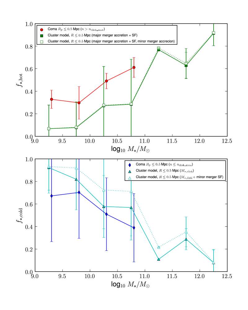
Figure 13: Top: The mean ratio of stellar mass fraction in dynamically hot components ($f_{\rm\star,hot}=M_{\rm\star,hot}/M_{\star}$) is plotted as a function of total galaxy $M_{\star}$. In the data, $M_{\rm\star,hot}$ is taken as the stellar mass of any high $n>n_{\rm disk\_max}$ classical bulge/elliptical component in the galaxy, excluding the cD galaxies (see Section 2.2). The model shown here is the best cluster model matched by cumulative galaxy number density (see Figure 10, column 1). For this model, the solid line takes $M_{\rm\star,hot}$ as the stellar mass built during major mergers, namely major merger stellar accretion plus induced SF, while the dashed line further adds in minor merger stellar accretion. Bottom: The mean stellar mass fraction in dynamically cold flattened components ($f_{\rm\star,cold}=M_{\rm\star,cold}/M_{\star}$) is plotted as a function of total galaxy stellar mass $M_{\star}$. In the data, $M_{\rm\star,cold}$ is taken as the stellar mass of any low $n\leq n_{\rm disk\_max}$ disk-dominated component in the galaxy. The model is represented by the solid and dashed lines. With the solid line we take $M_{\rm\star,cold}$ to be the mass of the outer disk $M_{\rm\star,Outer\_disk}$, which is given by ($M_{\star}-M_{\rm\star,Bulge,model}$). For the dotted line, we consider $M_{\rm\star,cold}$ to be the mass $M_{\rm\star,all\_disk}$ of inner and outer disks. We compute the latter mass as $M_{\rm\star,Outer\_disk}$ plus the mass of stars formed via induced SF during minor mergers. In both panels, only the projected central 0.5 Mpc of the clusters is considered. The error bars represent the $1\sigma$ standard deviation on the mean. The mean values for Coma are slightly offset in $M_{\star}$ for readability. The main conclusion is that the best-matching simulated clusters are underpredicting the mean fraction of $f_{\rm\star,hot}$ and overpredicting $f_{\rm\star,cold}$ over a wide range in galaxy stellar mass.

The comparison of R1_data with R2_model and R3_model is a global comparison of the total stellar mass fraction within high-$n$ components summed over all the galaxies with $M_{\star}\geq 10^{9}$ $M_{\odot}$. Next, we push the data versus model comparison one step further by doing it in bins of stellar mass, as shown in Figure 13.

The top panel of Figure 13 plots the mean ratio of stellar mass fraction in dynamically hot components ($f_{\rm\star,hot}$) as a function of total galaxy stellar mass, for data versus model. For each stellar mass bin shown in Figure 13, the value of $f_{\rm\star,hot}$ is calculated for each galaxy as $M_{\rm\star,hot}/M_{\star}$. In the data, $M_{\rm\star,hot}$ is taken as the stellar mass of any high $n>n_{\rm disk\_max}$ component in the galaxy. The model shown here is the best cluster model matched by cumulative galaxy number density (see Figure 10, column 1). For this model, two lines are shown: the solid line takes $M_{\rm\star,hot}$ as the stellar mass accreted and formed during major mergers, while the dotted line also adds in the stellar mass accreted during minor mergers.

In the top panel of Figure 13 there is significant disagreement between the fractions of $f_{\rm\star,hot}$ for the Coma data and the model. As shown by the second dotted model curve in Figure 13, adding in the stellar mass accreted in minor mergers to the model only changes the fraction by a few percent. The values of $f_{\rm\star,hot}$ are chiefly representative of the contributions from major mergers.

The bottom panel of Figure 13 plots the analogous mean ratio of stellar mass fraction in dynamically cold components ($f_{\rm\star,cold}=M_{\rm\star,cold}/M_{\star}$) as a function of total galaxy stellar mass. In the model, the two lines show two different expressions for $M_{\rm\star,cold}$. For the solid line, we take $M_{\rm\star,cold}$ to be the mass of the outer disk $M_{\rm\star,Outer\_disk}$, which represents the difference between the bulge mass ($M_{\rm\star,Bulge,model}$) and the total stellar mass. One problem with this approach is that it ignores small-scale nuclear disks formed in the bulge region. We tackle this problem by defining a second dotted model line that accounts for stars formed via induced SF during minor mergers. It is clear in the bottom panel of Figure 13 that the model overpredicts the mass in disks as a function of galaxy stellar mass. Note the contribution to $f_{\rm\star,cold}$ from minor merger induced SF is $\lesssim 17\%$ in a stellar mass given bin.

The main conclusion from Figure 13 is that the best-matching cluster model is underpredicting the mean fraction $f_{\rm\star,hot}$ of stellar mass locked in hot components over a wide range in galaxy stellar mass ($10^{9}\leq M\star\lesssim 8\times 10^{10}$ $M_{\odot}$). Similarly this model overpredicts the mean value for $f_{\rm\star,cold}$. The effect of cosmic variance on our sample (Section 4.2 and Appendix B.5) means our measured $f_{\rm\star,hot}$ is lower than the true value by an estimated factor of 1.16. Therefore, the underprediction of $f_{\rm\star,hot}$ in the model is worse than what we are citing. While the discussion in this section focused only on a single model cluster, the results and conclusions would be similar if we had analyzed alternate simulated clusters, such as those matched to the cluster galaxy stellar mass function (see Figure 10, column 2) or halo parameters (see Figure 10, column 3).

There could be several explanations as to why the models are underproducing the fraction of dynamically hot stellar mass ($f_{\rm\star,hot}$) and overproducing the fraction of dynamically cold stellar mass ($f_{\rm\star,cold}$). One possibility is that the absence of key cluster processes (especially ram-pressure stripping and tidal stripping) in the models is leading to the overproduction of the model galaxy’s cold gas reservoir (Section 5.5), compared to a real cluster galaxy, whose outer gas would be removed. This means that in the models, SF in gas that would otherwise be removed from the galaxy builds additional dynamically cold stellar mass following the last major merger. Another possibility is that the models ignore the production of bulges via the merging of star forming clumps (Bournaud, Elmegreen, & Elmegreen 2007; Elmegreen et al. 2009). It is still debated whether this mode can efficiently produce classical bulges, but if it does, then its non-inclusion in the models could lead to the underprediction of $f_{\rm\star,hot}$.

In summary, our comparison of empirical results to theoretical predictions underscores the need to include in SAMs environmental processes, such as ram-pressure stripping and tidal stripping, which affect the cold gas content of galaxies, as well as more comprehensive models of bulge assembly. It is clear that galaxy evolution is a function of both stellar mass and environment.

6 Summary & Conclusions

We present a study of the Coma cluster in which we constrain galaxy assembly history in the projected central 0.5 Mpc by performing multi-component structural decomposition on a mass-complete sample of 69 galaxies with stellar mass $M_{\star}\geq 10^{9}$ $M_{\odot}$. Some strengths of this study include the use of superb high-resolution ($0\hbox{$.\!\!^{\prime\prime}$}1$), F814W images from the HST/ACS Treasury Survey of the Coma cluster, and the adoption of a multi-component decomposition strategy where no a priori assumptions are made about the Sérsic index of bulges, bars or disks. We use structural decomposition to identify the two fundamental kinds of galaxy structure – dynamically cold, disk-dominated components and dynamically hot classical bulges/ellipticals – by adopting the working assumption that the Sérsic index $n$ is a reasonable proxy for tracing different structural components. We define disk-dominated structures as components with a low Sérsic index $n$ below an empirically determined threshold value $n_{\rm disk\_max}\sim 1.7$ (Section 3.1). Galaxies with an outer disk are called spirals or S0s. We explore the effect of environment by performing a census of disk-dominated structures versus classical bulges/ellipticals in Coma. We also compare our empirical results on galaxies in the center of the Coma cluster with theoretical predictions from a semi-analytical model. Our main results are summarized below.

1. Breakdown of stellar mass in Coma between low-$n$ disk-dominated structures and high-$n$ classical bulges/ellipticals:
   We make the first attempt (Section 4.2 and Tables 7–8) at exploring the distribution of stellar mass in Coma in terms of dynamically hot versus dynamically cold stellar components. After excluding the 2 cDs because of their uncertain stellar masses, we find that in the projected central 0.5 Mpc of the Coma cluster, galaxies with stellar mass $M_{\star}\geq 10^{9}$ $M_{\odot}$ have 57% of their cumulative stellar mass locked up in high-$n$ ($n\gtrsim 1.7$) classical bulges/ellipticals while the remaining 43% is in the form of low-$n$ ($n\lesssim 1.7$) disk-dominated structures (outer disks, inner disks, disky pseudobulges, and bars). Accounting for the effect of cosmic variance and color gradients in calculating these stellar mass fractions would not significantly change this census (Appendices B.5–B.6).
   

2. Impact of environment on morphology-density relation:
   Using our structural decomposition to assign galaxies the Hubble types E, S0, or spiral, we find evidence of a strong morphology-density relation. In the projected central 0.5 Mpc of the Coma cluster, spirals are rare, and the morphology breakdown of (E+S0):spirals is (91.0%):9.0% by numbers and (94.2%):5.8% by stellar mass (Section 4.1 and Table 6).
   

3. Impact of environment on outer disks:
   In the central parts of Coma, the properties of large scale disks are likely indicative of environmental processes that suppress disk growth or truncate disks (Section 4.5). In particular, at a given galaxy stellar mass, outer disks are smaller by $\sim 30-82\%$ and fainter in the $i$-band by $\sim 40-70\%$ (Figure 5). The suggestion that outer disks in Coma are more compact is consistent with the results of previous analyses of disk structure in Coma (Gutiérrez et al. 2004; Aguerri et al. 2004).
   

4. Impact of environment on bulges:
   The ratio $R$ of stellar mass in high-$n$ ($n\gtrsim 1.7$) classical bulges to low-$n$ ($n\lesssim 1.7$) disky pseudobulges is 17.3 in Coma. We measure $R$ to be a factor of $\sim 2.2-2.7$ higher in Coma compared with various samples from LDEs (Sections 4.2–4.3, Tables 7–8). We also find that at a given bulge Sérsic index $n$, the bulge-to-total ratio $B/D$, and the $i$-band light ratio are offset to higher values in Coma compared with LDEs. This effect appears to be due, at least in part, to the above-mentioned lower disk luminosity in Coma.
   

5. Comparison of data to theoretical predictions:
   We compare our empirical results on galaxies in the center of the Coma cluster with theoretical predictions based on combining the Millennium cosmological simulations of dark matter (Springel et al. 2005) with baryonic physics from a semi-analytical model (Neistein & Weinmann 2010; Wang, Weinmann, & Neistein 2012).

   It is striking that no model cluster can simultaneously match the global properties (halo mass/size, cumulative galaxy number density, galaxy stellar mass function) of Coma (Figures 9 and 10), and the cold gas to stellar mass ratios in the model clusters are at least 25 times higher than is measured in Coma.

   As suggested by Hopkins et al. (2009b), we find galaxy merger history is highly dependent on how the merger mass ratio $M_{1}/M_{2}$ is defined. Specifically, there is a factor of $\sim 5$ difference in merger rate when the merger mass ratio is based on the baryonic mass versus the stellar mass (Figure 11). Traditionally, observers have tended to use stellar mass ratios in identifying mergers, but with the advent of ALMA, it will be increasingly possible and important to incorporate the cold gas mass.

   For representative “best-match” simulated clusters, we compare the empirical and theoretically predicted fraction $f_{\rm\star,hot}$ and $f_{\rm\star,cold}$ of stellar mass locked, respectively, in high-$n$, dynamically hot versus low-$n$, dynamically cold stellar components. Over a wide range of galaxy stellar mass ($10^{9}\leq M\star\lesssim 8\times 10^{10}$), the model underpredicts the mean fraction $f_{\rm\star,hot}$ of stellar mass locked in hot components by a factor of $\gtrsim 1.5$. Similarly, the model overpredicts the mean value for $f_{\rm\star,cold}$ (Section 5.6 and Figure 13).

   We suggest this disagreement might be due to two main factors. Firstly, key cluster processes (especially ram-pressure stripping and tidal stripping), which impact the cold gas content and disk-dominated components of galaxies, are absent. Secondly, the models ignore the production of bulges via the merging of star forming clumps (Bournaud, Elmegreen, & Elmegreen 2007; Elmegreen et al. 2009). These results underscore the need to implement in theoretical models environmental processes, such as ram-pressure stripping and tidal stripping, as well as more comprehensive models of bulge assembly. It is clear that galaxy evolution is not a solely a function of stellar mass, but it also depends on environment.

Appendix A Using GALFIT

The proper operation of GALFIT depends on certain critical inputs. We briefly describe below how these important inputs are handled:

1. Point Spread Function (PSF):
   Accurate modeling of the PSF is essential in deriving galaxy structural properties. GALFIT convolves the provided PSF with the galaxy model in each iteration before calculating the $\chi^{2}$. Because the PSF varies with position across the ACS/WFC chips, it is ideal to separately model the PSF for each galaxy position. We use the grid of model ACS PSFs in the F475W and F814W filters from Hoyos et al. (2011). This grid of PSFs was created with TinyTim (Krist 1993) and DrizzlyTim.

   For a given set of multidrizzle parameters, DrizzlyTim transforms $x-y$ coordinates in the final science frames back to the system of individually distorted FLT images. DrizzlyTim invokes TinyTim to create a PSF with the specified parameters (e.g., position and filter) and then places the PSF at the appropriate position in blank FLT frames. The FLT frames are passed through MULTIDRIZZLE with the same parameters as the science images. Finally, a Charge Diffusion Kernel is applied to the PSFs in the geometrically distorted images. The grid of ACS PSFs from Hoyos et al. (2011) models a PSF for every 150 pixels in the $x$ and $y$ directions. For each galaxy in our sample we select the model PSF closest in proximity to the galaxy.

2. Sigma Images:
   A sigma image is the 2D map of the $1\sigma$ standard deviations in pixel counts of the input image. GALFIT uses the sigma image as the relative weight of pixels for calculating the goodness of fit. Achieving a reduced $\chi^{2}\sim 1$ with a successful model fit requires that the sigma image be correct. A sigma image can either be provided, or GALFIT can be allowed to calculate one based on the properties of the data image (image units of counts or counts/second, effective gain, read noise, number of combined exposures). We choose the latter option and allow GALFIT to calculate the sigma images.

3. Background Subtraction:
   While it is possible for GALFIT to freely fit the background sky, this is not recommended (Peng et al. 2002). In a multiple-component fit to a galaxy with at least two components, freely fitting the sky can exaggerate or suppress the wings of the central Sérsic profile and incorrectly measure the bulge half-light radius and Sérsic index. To avoid this, for each galaxy the background sky is measured and held fixed during the fit. The sky background is based on ellipse fitting with the IRAF/ELLIPSE task. Ellipses are fit to the galaxy and the surrounding area, with the ellipses in the surrounding area being fixed to the shape and orientation of the galaxy. The gradient along the semi-major axis is calculated, and the sky is estimated as the mean of elliptical annuli over a span in semi-major axis where the gradient reaches a prescribed small value. In each case, the area fitted by the ellipses exceeds the area subtended by the galaxy. Visual inspection of the ellipse fits shows that the perceived flat gradient corresponds to empty sky and not an extended galaxy outer profile with a very small gradient.

4. Image Thumbnails and Masks:
   Thumbnail cutouts of the intermediate-mass galaxies are made to lessen the computational time for fitting. Following Hoyos et al. (2011), square image thumbnails centered on the target galaxy are made using the output from SExtractor. Image size in pixels is determined with

   $$\rm{size=4\times A\_IMAGE\times KRON\_RADIUS}.$$ (8)

   The image units are transformed from counts/second to counts by multiplying by the exposure time. Image masks are based on the segmentation images provided from SExtractor. The segmentation images are modified to unmask the background and target galaxy being fitted. Any bright sources that visibly overlap with the target galaxy are also unmasked so that overlapping sources can be fitted simultaneously. Masks for relatively bright sources that do not overlap with the galaxy being fitted are expanded in semi-major axis by a factor of 1.5. We visually check by blinking the data image and modified segmentation image to verify that the unmasked region encompasses all of the target galaxy, including those with large diffuse halos that SExtractor does not capture (Hoyos et al. 2011).

Appendix B Details of Structural Decomposition

This appendix contains the full details concerning the structural decomposition scheme outlined in Section 3.2.

B.1 Single Sérsic Fits

We first fit all galaxies with a single Sérsic profile before attempting the multi-component fits. This step is useful for measuring the total luminosity of a galaxy as well as measuring the centroid (Weinzirl et al. 2009). The Sérsic profile has seven free parameters: centroid, luminosity, half-light radius $r_{\mathrm{e}}$, Sérsic index $n$, axis ratio, position angle, and diskiness/boxiness. We fix the diskiness/boxiness so that the fitted structures are perfect ellipses. We estimate the other six parameters based on the parameters in SExtractor and allow them to optimize in the fit. The detailed image preparation and inputs for the proper operation of GALFIT are described in Appendix A.

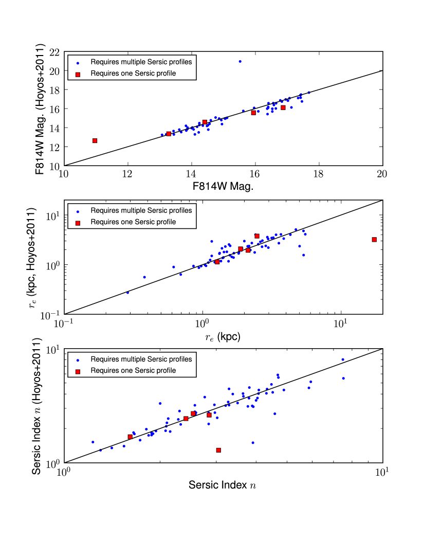
Figure 14: This figure compares our results for the single Sérsic fits (with no points source) with those obtained by Hoyos et al. (2011) using GALFIT on the same data. The sources in our sample requiring one Sérsic component are labeled separately from sources requiring two or three Sérsic profiles. Our derived magnitudes, $r_{\mathrm{e}}$, and $n$ for the sources requiring one Sérsic profile agree well with the parameters from Hoyos et al. (2011), with the one exception being cD galaxy NGC 4874 (COMAi125935.698p275733.36) with $n\sim 3$. Note that cD galaxy NGC 4889 requires only one Sérsic profile but it is not included here as it is not in the Hoyos et al. (2011) sample. See Appendix B.1 for additional details.

Figure 14 compares our results for the single Sérsic fits (with no point source) with those of Hoyos et al. (2011), who also perform single Sérsic fits with GALFIT and GIM2D using Coma ACS Treasury Survey data. Note that the galaxies in our sample requiring one Sérsic profile are distinguished in Figure 14. With the exception of COMAi125935.698p275733.36 (NGC 4874), our results for these sources requiring one Sérsic profile well match those derived by Hoyos et al. (2011). For NGC 4874, we measure the $r_{\mathrm{e}}$ and $n$ of NGC 4874 to be 17.3 kpc and 3.05, respectively, while Hoyos et al. (2011) measure $r_{\mathrm{e}}$ and $n$ to be 3.2 kpc and 1.3.

For sources requiring more than one Sérsic profile, our single Sérsic magnitudes agree well in general with those of Hoyos et al. (2011), except for one case (COMAi13051.149p28249.90) where Hoyos et al. (2011) underestimate the magnitude by $\sim 5.5$ mag. There are also outliers in both $r_{\mathrm{e}}$ and $n$. In 10 (5) instances (including COMAi13051.149p28249.90), the difference in $r_{\mathrm{e}}$ ($n$) exceeds a factor of 1.5.

There are two key differences in our fitting methodology (see Appendix A) compared with Hoyos et al. (2011). Most importantly, we entirely unmask the target galaxy and background in the segmentation-based masks so that GALFIT fits to pixels beyond what SExtractor associates with each galaxy. Hoyos et al. (2011) confine a galaxy to a customized mask generated based on the output of SExtractor. This approach misses a finite fraction of the flux in the target galaxy. This may explain why in Figure 14 we measure brighter magnitudes and larger $r_{\mathrm{e}}$ for more extended galaxies, where SExtractor does not detect all of the light in the galaxy. Second, we measure and fix the background sky while Hoyos et al. (2011) keep the sky as a free parameter. Allowing the sky background to freely vary in our fits fails to account for most of the scatter between our results and those of Hoyos et al. (2011). Rather, the disagreement appears to mainly be the result of differences in image masking.

B.2 Multi-Component Fits

For the Stage 2 Sérsic + Sérsic fits, we model the ‘inner’ and ‘outer’ components (C1 and C2) with Sérsic profiles that can represent physically different components (see Section 3.2).

Sensible initial guess parameters for Stage 2 are determined from a combination of the data image, Stage 1 model, and Stage 1 residuals. Guesses for the inner Sérsic component (C1) are usually based on the Stage 1 model. The centroid of the Sérsic components (and nuclear point source if present) are fixed to the best-fit centroid from the single Sérsic model. During the fits, we allow all other parameters (luminosity, $r_{\mathrm{e}}$, $n$, axis ratio, and position angle) to vary for the inner and outer components without a priori fixing the nature of these components.

With one exception, the $\chi^{2}$ in Stage 2 is always lower compared with $\chi^{2}$ in Stage 1 due to the extra Sérsic component. While the rare increase in $\chi^{2}$ from Stage 1 to Stage 2 is an indication the latter model is not reliable, the almost universal decrease in $\chi^{2}$ is not necessarily a sign that the Stage 2 fit is meaningful because, in principle, such a decrease in $\chi^{2}$ could be driven by the extra free model parameters. We consider a Stage 2 multi-component model to be superior to the Stage 1 fit if i) $\chi^{2}$ drops, ii) the Stage 2 model parameters are well behaved (i.e., not unphysically large or small), and iii) the Stage 2 residuals are deemed by visual inspection to show a reduction in coherent structure relative to the Stage 1 residuals.

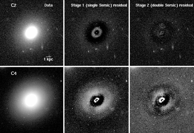
Figure 16: This figure shows how some of the galaxies (C2$=$COMAi125935.286p275149.13 and C4$=$COMAi13014.746p28228.69) poorly fitted by a single Sérsic model (plus point source if needed) in Stage 1 can be better fitted by two Sérsic models (plus point source if needed) in Stage 2. Each row shows the data, residual after Stage 1, and the residual after Stage 2. Galaxy C2 is best-fit as having an inner disk ($n=0.31$) and an outer elliptical structure ($n=2.08$). Galaxy C4 is best fit with an inner bulge $n=3.68$ and an outer disk ($n=0.47$).

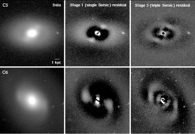
Figure 17: This figure shows two examples of barred galaxies (C5$=$COMAi13027.966p275721.56 and C6$=$COMAi125930.824p275303.05) poorly fitted by a Stage 1 single Sérsic model that are better fitted by a Stage 3 triple Sérsic (plus point source if needed) model. Column 1 shows the data images while columns 2 and 3 show the residuals after the Stage 1 and Stage 3 model, respectively.

Figure 15 provides examples where a single Sérsic model fails to model the entire galaxy well and leaves behind coherent structure in the residuals. Such coherent structure is indicative of additional components such as compact central structures, rings, annuli and extended components, and bars/ovals. We illustrate in Figures 16 and 17 how some of these examples are best fitted by models with multiple Sérsic components.

If a galaxy does not require a Stage 2 model, or if the Stage 2 model fails to meet the above criteria, then the galaxy is described by a single Sérsic profile + point source, if present. Six galaxies are best represented by Stage 1. Two (COMAi13017.683p275718.93 and COMAi13018.093p275723.59) cannot be fit with multiple Sérsic models because they are interacting. In the third case, (COMAi125931.103p275718.12), the $\chi^{2}$ increases from Stage 1 to Stage 2. The final three cases (NGC 4874, NGC 4889, and COMAi125909.468p28227.35) show evidence of a core (see Appendix C).

Galaxies for which the Stage 2 model is deemed an improvement are interpreted as follows. Since the outer component C2 could represent a disk, we must specify criteria for identifying an outer disk. The outer component C2 is a disk if it satisfies at least one of the following. i) The galaxy is highly inclined such that C2 has a low axis ratio $b/a\leq 0.25$ that is below the axis ratios found for ellipticals. ii) The galaxy is moderately inclined and C2 shows disk signatures (e.g., bars, rings, or spiral arms) in the data images and/or Stage 2 residuals. iii) For moderately inclined galaxies without disk features that do not satisfy (i) or (ii), we require Sérsic $n$ be less than the threshold value $n_{\rm disk\_max}$.

Theoretical considerations show that pure disks have $n=1$, suggesting the threshold should be $n\sim 1$. However, real galaxy disks are not fitted perfectly by Sérsic profiles. We determine the value empirically from the maximum disk Sérsic index in galaxies satisfying (i) and (ii). Highly inclined disks show a range in Sérsic index of 0.48-0.86. Moderately inclined galaxies identified as having spiral arms but no bar have outer disks with Sérsic index 0.63-1.20. Note that some of the highly inclined galaxies could be barred, and this may may account for the small difference in average Sérsic index between the highly inclined and moderately inclined barred galaxies.

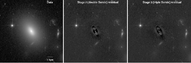
Figure 18: This figure shows the decomposition of moderately inclined, barred galaxy COMAi125950.105p275529.44, in which we measure the highest outer disk Sérsic index $n=1.66$. Thus, this galaxy sets the empirically determined upper limit on disk Sérsic index, $n_{\rm disk\_max}=1.66$. Column 1 shows the data images while columns 2 and 3 show the residuals for the Stage 2 and Stage 3 model, respectively. The bar signature is clearly present in the residuals.

In order to accurately model the outer disk of moderately inclined barred galaxies, a triple Sérsic profile (see below) is required. After taking this extra step, the outer disk Sérsic index among moderately inclined barred galaxies is 0.25-1.66. The maximum Sérsic index among outer disks in galaxies satisfying requirement (i) and (ii) is 1.66, and we therefore set $n_{\rm disk\_max}$ to this value. Thus, outer disks span the range 0.25-1.66 in Sérsic index and have a median $n$ of 0.84. Figure 18 shows the galaxy (COMAi125950.105p275529.44) on which we base our measurement of $n_{\rm disk\_max}$. Appendix D discusses the uncertainties in the adopted value of $n_{\rm disk\_max}$.

Galaxies that satisfy any of requirements (i), (ii), or (iii) are deemed to have an outer disk. Galaxies without an outer disk are considered photometric ellipticals.

We test all galaxies having an outer disk for the presence of a large-scale bar/oval in Stage 3 by fitting a triple Sérsic profile + point source, if present. Bars/ovals are modeled with an elongated, low Sérsic index ($n\sim 0.5$) profile (Peng et al. 2002; Weinzirl et al. 2009). In the text, we do not distinguish between bars and ovals, and we use “bar” to describe both.

The initial guesses for the three-component models come from the best Stage 2 model combined with visual inspection. The Sérsic index for the bar is initially guessed to be 0.5, and the shape and position angle of the bar are visually estimated using the data image or the residuals of the Stage 2 fit. When selecting between the Stage 2 and Stage 3 fits, we applied the same constraints described above for the behavior of $\chi^{2}$. An additional complication is that in galaxies with unbarred outer disks, GALFIT may fit a ‘bar’ to any existing spiral arms, rings, or clumpy disk structure. Stage 3 fits in these cases could be discarded by noting the resulting discrepancies in appearance between the galaxy images and the Stage 3 model images. Figure 17 shows examples of two disk galaxies where adding the third Sérsic component removes the bar signature from the residuals.

B.3 Nuclear Point Sources

Nuclear point sources are found in galaxies of all Hubble types. The frequency of nuclear point sources is very sample dependent and is particularly sensitive to range of galaxy luminosity. HST studies of early-type galaxies (e.g., Ravindranath et al. 2001; Côté et al. 2006) have measured nucleation rates of $50\%$ or more. Ravindranath et al. (2001) find about half of early-type (E, S0, S0/a) galaxies have nuclear point sources. Côté et al. (2006) show that the frequency of nucleation in ACS images of the Virgo cluster is at least 66% in galaxies with $M_{B}\leq-15$. Graham & Guzmán (2003) discuss 13/15 examples of dwarf ellipticals in the Coma cluster showing evidence for nucleation. Balcells et al. (2007a) measure a frequency of 58% for S0 to Sbc galaxies. Böker et al. (2002) measure the frequency of point sources to be 75% in spirals with Hubble types Scd to Sm.

Although nuclear point sources account for a small percentage ($<1\%$) of a galaxy’s light, it is important to include them during multi-component structural decomposition. Neglecting nuclear point sources can have a significant effect on derived parameters of bulges (Balcells et al. 2003; Weinzirl et al. 2009). We assess the presence of nuclear point sources with visual inspection. If a compact light source is visible by eye in the residuals of the single Sérsic fit, the galaxy is flagged as having a potential point source. With this procedure, 49/69 galaxies in sample S2 have a potential nuclear point source.

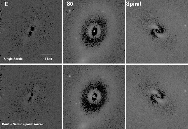
Figure 19: This figure compares residuals after fitting a single Sérsic model (top row) versus the best fit double Sérsic + nuclear point source model (bottom row) for an elliptical (COMAi13030.954p28630.22), S0 (COMAi13021.673p275354.81), and spiral (COMAi13041.193p28242.34). The nuclear point source is visible in the residuals in the top row.

Galaxies having a potential nuclear point source are fitted with an extra nuclear point source component in the best-fit single or multi-component model. GALFIT models the point source with the user-input PSF. More than half (38/69, $55.1\pm 6.0\%$) of objects in sample S2 have a nuclear point source in the final, best-fit structural decomposition. Figure 19 shows examples of residual galaxy images with point sources.

Figure 20 shows the derived point source luminosities correlate with total galaxy magnitude such that more luminous point sources are found in brighter galaxies. Similar results been found in earlier work (e.g., Graham & Guzmán 2003; Balcells et al. 2007a).

B.4 cD Galaxies

cD galaxies are defined by having extra light on cluster-sized ($\sim 1$ Mpc) scales with respect to the outward extrapolation of the Sérsic profile fit to the inner ($\sim 100$ kpc) portion of the galaxy. Such galaxies are luminous and are found in regions of high galaxy number density (Binney & Merrifield 1998). Of the three cD galaxies in Coma, two (NGC 4874 and NGC 4889) lie in the projected central 0.5 Mpc and are therefore in our sample. The third cD (NGC 4839) lies is in the outer southwest region of Coma and is not part of this study.

Definitive proof that NGC 4874 and NGC 4889 are cDs is the detection of intra-cluster light in Coma (Kormendy & Bahcall 1974; Melnick et al. 1977; Thuan & Kormendy 1977; Bernstein et al. 1995; Adami et al. 2005; Arnaboldi 2011).

The single Sérsic indices reported in Appendix B and Table 3 for the these cD galaxies are $n\sim 3-4.4$ because the decompositions also include the central core. The central core is a clear deviation from the inward extrapolation of the Sérsic profile that characterizes the outer galaxy structure. For this reason, masking the core regions (i.e., the central $\sim 2^{\prime\prime}$) is more physically motivated and would yield higher single Sérsic indices $n\gtrsim 8$. This is demonstrated in Appendix C and Table 2. We note that both approaches (masking or not masking the core during the $2D$ decomposition) lead us to the same conclusion that all of the cD light is associated with structures of $n\gg n_{\rm disk\_max}$ (Appendix C). Note in Table 5 we list the cD galaxies the structure parameters from the 2D decomposition where the core is masked.

The high $n\gg n_{\rm disk\_max}$ values in the cD galaxies are due to the extended wings in the Sérsic profile resulting from the extended low surface brightness envelope of the cD. This extended envelope is likely made up of intra-cluster light and the cumulative debris from galaxies, consistent with the view that cD galaxies arise from repeated bouts of galactic cannibalism and tidal stripping of satellite galaxies in a cluster (Ostriker & Tremaine 1975; Aragon-Salamanca et al. 1998; De Lucia & Blaizot 2007).

B.5 Cosmic Variance

The Coma ACS data only cover 19.7% of the projected central 0.5 Mpc radius of Coma. The relative fractional numbers of E+S0:spiral, or specifically the ratio of E/S0s, we derive from this data may not be representative of the full region in the projected central 0.5 Mpc radius of Coma due to the incomplete sampling and cosmic variance. In order to assess the effect of incomplete sampling and cosmic variance on our results, we perform the following test.

First, we define the region covered by ACS in the projected central 0.5 Mpc radius of Coma as R1, and the full area in the projected central 0.5 Mpc radius of Coma as R2. We use the Hubble morphological types (MT) from the GOLD Mine database (Gavazzi et al. 2003) to compute the fraction of E+S0:spiral galaxies in region R1 and R2 with $M_{\star}\geq 4.4\times 10^{9}$ $M_{\odot}$, the mass limit of the Coma GOLD Mine sample. The MT reported by GOLD Mine are sourced from the literature. If we take the visual MT from GOLD Mine at face value then we draw the following conclusions:

1. The effect cosmic variance causes the ratio of E/S0 within the GOLD Mine MT to vary by a factor of 1.11 between region R1 and R2 for $M_{\star}\geq 4.4\times 10^{9}$ $M_{\odot}$.

2. The partial ACS coverage of the projected central 0.5 Mpc and associated cosmic variance thus causes our study based on region R1 to

   1. overestimate the ratio of S0/E in the ACS sample for $M_{\star}\geq 4.4\times 10^{9}$ $M_{\odot}$ by a factor of 1.4.

   2. overestimate the fraction $f_{\rm cold}$ of dynamically cold stellar mass (43%) by a factor of 1.27 (Section 5.6) for $M_{\star}\geq 10^{9}$ $M_{\odot}$. We note that the over-estimation of $f_{\rm cold}$ is not by the same factor as in ii (a) because S0s have a significant fraction of their mass in dynamically hot bulges.

3. Currently, our conclusion in Section 5.6, based on region R1 is that the hierarchical models are over-predicting the empirical fraction $f_{\rm cold}$. It is clear from ii (b), that correcting for partial ACS coverage and cosmic variance would only strengthen this conclusion further.

B.6 Galaxy Color Gradients

In Section 4.2 we suggest that galaxy color gradients should not bias our conclusions concerning the distribution of dynamically hot and cold stellar mass. Here, we explicitly test this idea.

For a subset of 10 galaxies spanning types G3 to G5 and matching the morphology distribution of the mass-selected sample (E+S0:spiral = 2+7:1) in Table 6, we re-evaluated the fractional mass in hot and cold components based on combining structural decompositions of both the F814W and F475W images. The new F475W-band decompositions were performed identically to the existing F814W decompositions, except that the position angle and axis ratio of the galaxy structures were fixed to their values from the F814W-band decompositions. Stellar masses of the structural components were calculated according to Into & Portinari (2013) after converting the F475W-F814W color and the F814W luminosity into a $B-I$ color and $I$-band luminosity, respectively, using the procedure in Section 2.2.

In the new F475W decompositions for this subset of galaxies, the half-light radii and Sérsic $n$ are similar to the corresponding values in the F814W band. The average offset is 5.4% with a standard deviation of 5.6%. Furthermore, the fractional hot stellar mass inferred from a constant global F814W $M/L$ ratio is 53.4%. After calculating the stellar mass of each galaxy component from the $B-I$ color, the fractional hot stellar mass is found to be 50.5%. Thus, $M/L$ gradients within a galaxy do not appear to have a significant effect on the fractional masses measured in cold versus hot components.

Appendix C Identifying Core Ellipticals

While elliptical galaxies are remarkably well-fit by Sérsic profiles over large dynamic ranges, giant elliptical galaxies contain cores, or “missing light” at small radii that constitute a downward deviation from from the inward extrapolation of the outer Sérsic profile (Graham et al. 2003; Trujillo et al. 2004; Kormendy et al. 2009). Such cores are hypothesized to form from scouring induced by binary black holes during dry, dissipationless mergers.

Because cores, which have traditionally been identified with 1D radial light profiles, are not an obvious feature of the galaxy’s 2D light distribution, global Sérsic fits will encompass any existing core. This is potentially problematic for at least two reasons. Including the core in the Sérsic fit will lower the global Sérsic index. This is of concern in this paper where the Sérsic index plays a key role in interpreting galaxy structure (Section 3.1). Secondly, fitting the core region may produce features in the residuals that prompt addition of extra nuclear components that have no physical justification.

We systematically search for cores in all sample galaxies. For this task, we use 1D light profiles generated from ellipse fitting of deconvolved images. The ACS images were deconvolved using a simulated PSF (Appendix A for details) and 40 iterations of Lucy-Richardson deconvolution with the IRAF task LUCY (Lucy 1974; Richardson 1972). Our approach uses the criteria for identifying core galaxies from Trujillo et al. (2004) by fitting Sérsic and core-Sérsic profiles (Graham et al. 2003) to the 1D light profiles.

For simplicity, we use the version of the core-Sérsic profile that assumes an infinitely sharp transition between the outer Sérsic and inner power-law regions, namely

$$\rm{I(r)=I_{b}[(r_{b}/r)^{\gamma}u(r_{b}-r)+e^{b(r_{b}/r_{\mathrm{e}})^{1/n}}e^{-b(r/r_{\mathrm{e}})^{1/n}}u(r-r_{b})]}.$$ (9)

Here, $r_{b}$ denotes the division between the outer Sérsic and inner power-law profiles, $I_{b}$ is the intensity at this radius, $\gamma$ is the inner power-law slope, and $u(x-a)$ is the Heaviside step function. Parameters $n$ and $r_{\mathrm{e}}$ refer to the shape and half-light radius of the outer Sérsic profile. Additionally, $b$ is a constant that depends on several free parameters ($r_{b}$, $\gamma$, $r_{\mathrm{e}}$, and $n$).

We require a core galaxy to meet the following criteria: 1) the core-Sérsic model provide a better fit than the Sérsic profile; 2) the cores are well-resolved so that the break radius $r_{b}$ is greater than the second innermost data point in the profile; 3) the inner power-law slope $\gamma$ is less than the logarithmic slope of the Sérsic profile ($1/n$) in the core region.

Three sample galaxies meet the above criteria for having a core. Two of these are the central cD galaxies NGC 4874 and NGC 4889. Table 2 summarizes the $r_{b}$ and $\gamma$ measured from the core-Sérsic fit.

We further explore the best way to handle these cored galaxies in the 2D luminosity decompositions. Two natural approaches are to fit the whole galaxy, including the core, or to mask the galaxy over $r\leq r_{b}$. Masking is more physically motivated because the central core is a clear deviation from the inward extrapolation of the Sérsic profile that characterizes the outer galaxy structure. We try both approaches and summarize the results in Table 2. Applying a mask versus no mask has a nominal effect on COMAi125909.468p28227.35, but there is a significant increase in the $r_{\mathrm{e}}$ and $n$ of the cD galaxies when their larger core regions are masked.

Performing the 2D fit with the core masked is more physically motivated, and we consider these models to represent the best fits for the cD galaxies. It is worth noting, however, that our result from Appendix B.4 that 100% of the mass in the cDs is associated with structures of $n\gg n_{\rm disk\_max}$ remains unchanged irrespective of which approach (mask or no mask) we take.

Appendix D Systematics of ${n_{\rm disk\_max}}$

Our effort in this paper to make a census (Section 4.2) of dynamically cold versus dynamically hot stellar mass depends fundamentally on the upper limit, $n_{\rm disk\_max}$ (Section 3.1), measured for the Sérsic index of a disk. In our approach, all structures with Sérsic index $n\leq n_{\rm disk\_max}$ are considered disk dominated, while all other structures with higher Sérsic index are considered classical components built in mergers.

The value of $n\leq n_{\rm disk\_max}$ is set by the moderately inclined barred galaxy (COMAi125950.105p275529.44) having the highest outer disk Sérsic index. The accuracy of $n_{\rm disk\_max}$ depends on how representative the sample is as well as the robustness of the multi-component structural decompositions. Figure 18 shows for this galaxy the data image and residuals of the multi-component decompositions. While this galaxy was identified as an ambiguous E/S0 galaxy in Figure 2 of Marinova et al. (2012), the barred nature of this galaxy seems clear based on the image residuals produced by our improved method (Sections 3.2 and 3.3) of structural decomposition.

The value of $n_{\rm disk\_max}$ is subject to sky subtraction errors because it is measured from the outermost Sérsic profile of disk galaxies, and this is likely the dominant systematic effect on $n_{\rm disk\_max}$. As described in Appendix A, we measure the background sky value with a robust method and hold the sky fixed at this value during the fit. To test the importance of the sky subtraction, we refitted COMAi125950.105p275529.44 while adjusting the mean sky background by $\pm 1\sigma$. This produces a range in outer disk $n$ of $n\sim 1.57-1.77$, which spans $\sim 0.1$ above and below the adopted $n_{\rm disk\_max}$ value of 1.66. Based on the narrow error bars for $n_{\rm disk\_max}$, we do not expect the uncertainty to have a significant impact on our conclusions.

For completeness, we explore for an alternate value of $n_{\rm disk\_max}$ the relative stellar mass fractions that would be interpreted as belonging to cold versus hot stellar components. The value $n_{\rm disk\_max}=2$ is in line with estimates of the Sérsic index of small-scale disks (e.g., Fisher & Drory 2008; Weinzirl et al. 2009) yet is still above the anticipated range in $n_{\rm disk\_max}$ due to sky subtraction errors in this study. With this higher $n_{\rm disk\_max}$, we would find that $\sim 51\%$ stellar mass is in disk-dominated components while $\sim 49\%$ is still in classical bulges/ellipticals assembled in major and minor mergers. These values are somewhat different from the corresponding values (43% in disk-dominated structures versus 57% in non-disks) derived in Section 4.2 excluding the 2 cD galaxies. Choosing a higher $n_{\rm disk\_max}$ would increase the importance of disk-building processes relative to processes that build classical bulges/ellipticals.

Table 1: Cross Identifications

Galaxy Name	SDSS DR8 Name	2MASS XSC (or PSC Name)	GMP Name	Dressler (1980) Name
(1)	(2)	(3)	(4)	(5)
COMAi125926.458p275124.81	1237667444048658752	-	GMP3473	-
COMAi13007.123p275551.49	1237667444048724242	2MASSJ13000711+2755511	GMP2931	-
COMAi125930.270p28115.17	1237667324334571563	-	GMP3406	-
COMAi125937.200p275819.97	1237667444048658537	2MASSJ12593720+2758203	GMP3308	-
COMAi125953.929p275813.75	1237667444048658918	-	GMP3098	-
COMAi13018.351p28333.32	1237667324334637348	-	GMP2787	-
COMAi125937.010p28106.95	1237667324334571551	2MASSJ12593699+2801074	GMP3312	-
COMAi125946.943p275930.90	1237667324334571832	2MASSJ12594688+2759308	GMP3166	-
COMAi13030.954p28630.22	1237667324334637213	2MASSJ13003091+2806300	GMP2626	-
COMAi13035.420p275634.06	1237667444048724352	-	GMP2585	-
COMAi125950.183p275445.52	1237667444048658912	-	GMP3131	-
COMAi125959.476p275626.02	1237667444048658878	-	GMP3034	-
COMAi13000.949p275643.85	1237667444048658882	2MASSJ13000095+2756433	GMP3017	-
COMAi13034.430p275604.95	1237667444048724349	2MASSJ13003442+2756047	GMP2591	-
COMAi125931.893p275140.76	1237667444048658763	2MASSJ12593186+2751406	GMP3383	-
COMAi125931.103p275718.12	1237667444048658549	-	GMP3392	-
COMAi13041.193p28242.34	1237667324334702866	2MASSJ13004119+2802424	GMP2529	-
COMAi125845.533p274513.75	1237667323797635368	2MASSJ12584558+2745132	GMP4035	-
COMAi13018.545p28549.62	1237667324334637356	2MASSJ13001857+2805503	GMP2784	-
COMAi13021.673p275354.81	1237667444048724303	2MASXJ13002172+2753545	GMP2736	-
COMAi13024.823p275535.94	1237667444048724320	2MASSJ13002482+2755353	GMP2692	-
COMAi13051.149p28249.90	1237667324334702708	2MASSJ13005112+2802499	GMP2423	-
COMAi13011.143p28354.91	1237667324334637325	2MASSJ13001117+2803551	GMP2879	-
COMAi125937.990p28003.52	1237667324334571647	2MASSJ12593798+2800036	GMP3292	-
COMAi13018.873p28033.38	1237667324334637362	2MASXJ13001890+2800332	GMP2777	-
COMAi125911.543p28033.32	1237667324334506328	2MASSJ12591153+2800334	GMP3681	-
COMAi125904.797p28301.16	1237667324334506316	2MASXJ12590475+2803019	GMP3780	-
COMAi125909.468p28227.35	1237667324334506325	2MASXJ12590943+2802279	GMP3707	-
COMAi125935.286p275149.13	1237667444048658774	2MASXJ12593524+2751488	GMP3339	-
COMAi13005.405p28128.14	1237667324334637091	2MASXJ13000538+2801282	GMP2960	-
COMAi125950.105p275529.44	1237667444048658822	2MASXJ12595013+2755292	GMP3133	-
COMAi13018.772p275613.34	1237667444048723991	2MASXJ13001877+2756135	GMP2778	-
COMAi125938.321p275913.89	1237667444048658535	2MASXJ12593827+2759137	GMP3291	D154
COMAi125940.270p275805.71	1237667444048658530	2MASSJ12594026+2758058	GMP3254	D127
COMAi125944.208p275730.38	1237667444048658531	2MASXJ12594423+2757307	GMP3206	D126
COMAi125939.659p275714.03	1237667444048658528	2MASSJ12593965+2757141	GMP3269	D128
COMAi13044.632p28602.31	1237667324334702891	2MASXJ13004459+2806026	GMP2489	D191
COMAi125928.721p28225.92	1237667324334571539	2MASXJ12592868+2802258	GMP3433	D177
COMAi125942.301p275529.15	1237667444048658653	2MASXJ12594234+2755287	GMP3222	D125
COMAi13017.014p28350.07	1237667324334637347	2MASXJ13001702+2803502	GMP2805	D171
COMAi125956.697p275548.71	1237667444048658858	2MASXJ12595670+2755483	GMP3068	D123
COMAi13016.534p275803.15	1237667444048723984	2MASXJ13001655+2758032	GMP2815	D122
COMAi13006.395p28015.94	1237667324334637086	2MASXJ13000643+2800142	GMP2940	D150
COMAi13027.966p275721.56	1237667444048724118	2MASXJ13002798+2757216	GMP2654	D119
COMAi13012.868p28431.74	1237667324334637140	2MASXJ13001286+2804322	GMP2861	D173
COMAi125943.721p275940.82	1237667324334571645	2MASSJ12594372+2759409	GMP3213	D153
COMAi13028.370p275820.64	1237667444048724328	2MASXJ13002835+2758206	GMP2651	D147
COMAi13042.832p275746.95	1237667444048724176	2MASXJ13004285+2757476	GMP2510	D116
COMAi13038.761p28052.34	1237667324334702605	2MASXJ13003877+2800516	GMP2551	D146
COMAi13014.746p28228.69	1237667324334637152	2MASXJ13001475+2802282	GMP2839	D172
COMAi13022.170p28249.30	1237667324334637189	2MASXJ13002215+2802495	GMP2727	D170
COMAi125931.453p28247.60	1237667324334571535	2MASXJ12593141+2802478	GMP3390	D176
COMAi13018.093p275723.59	1237667444048723985	2MASSJ13001809+2757235	GMP2794	D120
COMAi13040.838p275947.80	1237667324334702869	2MASXJ13004081+2759476	GMP2535	D145
COMAi125852.097p274706.15	1237667323797635203	2MASXJ12585208+2747059	GMP3958	D072
COMAi125946.782p275825.99	1237667444048658525	2MASXJ12594681+2758252	GMP3170	D152
COMAi13008.003p28442.81	1237667324334637131	2MASXJ13000803+2804422	GMP2922	D174
COMAi125929.956p275723.26	1237667444048658522	2MASSJ12592995+2757231	GMP3414	D131
COMAi125929.403p275100.46	1237667444048658609	2MASXJ12592936+2751008	GMP3423	D088
COMAi125932.771p275901.04	1237667444048658523	2MASXJ12593276+2759008	GMP3367	D155
COMAi125944.407p275444.84	1237667444048658654	2MASXJ12594438+2754447	GMP3201	D124
COMAi125930.824p275303.05	1237667444048658616	2MASXJ12593079+2753028	GMP3400	D103
COMAi13039.767p275526.19	1237667444048724135	2MASXJ13003975+2755256	GMP2541	D118
COMAi13042.766p275817.38	1237667324334702622	2MASXJ13004277+2758166	GMP2516	D144
COMAi13048.646p28526.69	1237667324334702681	2MASXJ13004867+2805266	GMP2440	D168
COMAi13017.683p275718.93	1237667444048723981	2MASXJ13001768+2757192	GMP2798	D121
COMAi13051.464p28234.86	1237667324334702705	2MASXJ13005158+2802341	GMP2417	D167
NGC 4889	1237667444048723983	2MASXJ13000809+2758372	GMP2921	D148
COMAi125935.698p275733.36 (NGC 4874)	1237667444048658532	2MASXJ12593570+2757338	GMP3329	D129
Notes. If there is no match in the 2MASS Extended Source catalog (2MASX), where available, the 2MASS Point Source catalog name (2MASS) is given in column (3). GMP name refers to the Godwin, Metcalfe, Peach (1983) catalog.

Table 2: Properties Of Cored Ellipticals

Galaxy Name	Core-Sérsic ($\gamma$, $r_{b}$)	2D Sérsic Profile w/o	2D Sérsic Profile w/
		Core Masked ($n$, $r_{e}$)	Core Masked ($n$, $r_{e}$)
(1)	(2)	(3)	(4)
COMAi125909.468p28227.35	(0.16, 0$.\!\!^{\prime\prime}$13)	(2.54, 4$.\!\!^{\prime\prime}$2)	(2.54, 4$.\!\!^{\prime\prime}$20)
NGC 4874 (ACS F814W)	(0.15, 1$.\!\!^{\prime\prime}$40)	(2.89, 35$.\!\!^{\prime\prime}$4)	(11.4, 875$.\!\!^{\prime\prime}$)
NGC 4874 (SDSS $i$-band)	(0.15, 2$.\!\!^{\prime\prime}$32)	(4.30, 88$.\!\!^{\prime\prime}$3)	(4.70, 107$.\!\!^{\prime\prime}$)
NGC 4889 (SDSS $i$-band)	(0.06, 1$.\!\!^{\prime\prime}$88)	(3.90, 42$.\!\!^{\prime\prime}$9)	(7.80, 129$.\!\!^{\prime\prime}$)
Notes. Galaxies are identified as having a core following the procedure in Appendix C. Two of the cored galaxies (NGC 4874 and NGC 4889) are cD galaxies.

Table 3: Galaxy Properties And Single Sérsic Profile Structural Parameters

Galaxy Name	RA	DEC	$M_{\star}$	F814W Magnitude	$r_{\mathrm{e}}$	$n$
			($M_{\odot}$)		(kpc)
(1)	(2)	(3)	(4)	(5)	(6)	(7)
COMAi125926.458p275124.81	194.860245	27.856893	1.03e+09	17.43	0.97	1.88
COMAi13007.123p275551.49	195.029679	27.930971	1.03e+09	17.42	0.62	2.76
COMAi125930.270p28115.17	194.876126	28.020883	1.05e+09	17.46	1.04	1.90
COMAi125937.200p275819.97	194.905001	27.972214	1.12e+09	17.68	0.29	4.51
COMAi125953.929p275813.75	194.974706	27.970489	1.17e+09	17.41	1.10	1.30
COMAi13018.351p28333.32	195.076465	28.059258	1.17e+09	17.13	1.32	1.23
COMAi125937.010p28106.95	194.904209	28.018598	1.23e+09	17.34	0.69	2.08
COMAi125946.943p275930.90	194.945597	27.991917	1.40e+09	17.02	1.49	1.65
COMAi13030.954p28630.22	195.128977	28.108396	1.46e+09	17.07	1.41	1.94
COMAi13035.420p275634.06	195.147586	27.942797	1.72e+09	16.83	1.92	1.81
COMAi125950.183p275445.52	194.959098	27.912647	1.81e+09	16.95	1.57	1.41
COMAi125959.476p275626.02	194.997820	27.940564	1.83e+09	16.53	2.41	2.30
COMAi13000.949p275643.85	195.003956	27.945514	1.92e+09	16.40	2.00	3.38
COMAi13034.430p275604.95	195.143461	27.934709	1.94e+09	16.65	2.11	2.10
COMAi125931.893p275140.76	194.882888	27.861324	1.96e+09	16.78	0.94	1.88
COMAi125931.103p275718.12	194.879597	27.955035	1.99e+09	16.87	2.47	1.61
COMAi13041.193p28242.34	195.171639	28.045097	2.15e+09	16.83	0.86	1.66
COMAi125845.533p274513.75	194.689724	27.753820	2.21e+09	16.56	2.14	2.09
COMAi13018.545p28549.62	195.077272	28.097119	2.25e+09	16.64	1.62	1.73
COMAi13021.673p275354.81	195.090308	27.898559	2.71e+09	16.37	1.46	2.57
COMAi13024.823p275535.94	195.103430	27.926652	2.73e+09	16.41	2.68	2.15
COMAi13051.149p28249.90	195.213122	28.047197	2.78e+09	15.52	5.35	3.17
COMAi13011.143p28354.91	195.046429	28.065253	2.83e+09	16.38	1.42	2.12
COMAi125937.990p28003.52	194.908292	28.000979	2.97e+09	16.53	1.16	2.00
COMAi13018.873p28033.38	195.078639	28.009273	2.98e+09	16.58	0.38	3.29
COMAi125911.543p28033.32	194.798099	28.009258	3.26e+09	16.40	1.22	1.84
COMAi125904.797p28301.16	194.769991	28.050323	3.78e+09	16.09	2.16	2.28
COMAi125909.468p28227.35	194.789451	28.040932	5.14e+09	15.94	1.88	2.54
COMAi125935.286p275149.13	194.897029	27.863650	5.27e+09	15.96	1.06	1.54
COMAi13005.405p28128.14	195.022521	28.024486	8.40e+09	15.11	2.61	2.58
COMAi125950.105p275529.44	194.958773	27.924845	8.88e+09	15.62	1.35	2.32
COMAi13018.772p275613.34	195.078218	27.937041	9.56e+09	15.09	3.23	2.57
COMAi125938.321p275913.89	194.909675	27.987192	9.96e+09	14.93	3.67	3.50
COMAi125940.270p275805.71	194.917794	27.968254	1.01e+10	15.04	2.52	5.94
COMAi125944.208p275730.38	194.934203	27.958439	1.20e+10	14.60	3.55	3.89
COMAi125939.659p275714.03	194.915246	27.953900	1.21e+10	15.05	1.33	3.65
COMAi13044.632p28602.31	195.185968	28.100644	1.38e+10	14.86	1.82	2.84
COMAi125928.721p28225.92	194.869671	28.040534	1.39e+10	14.95	1.67	2.97
COMAi125942.301p275529.15	194.926256	27.924765	1.61e+10	14.56	1.16	7.49
COMAi13017.014p28350.07	195.070896	28.063911	1.79e+10	14.75	1.35	3.91
COMAi125956.697p275548.71	194.986241	27.930200	1.82e+10	14.35	4.71	3.80
COMAi13016.534p275803.15	195.068895	27.967542	1.84e+10	14.24	2.98	4.58
COMAi13006.395p28015.94	195.026649	28.004430	1.87e+10	13.82	5.01	7.52
COMAi13027.966p275721.56	195.116526	27.955989	2.11e+10	14.51	1.55	4.68
COMAi13012.868p28431.74	195.053620	28.075485	2.11e+10	14.52	1.40	3.21
COMAi125943.721p275940.82	194.932172	27.994675	2.13e+10	14.48	1.38	3.81
COMAi13028.370p275820.64	195.118212	27.972400	2.17e+10	14.24	4.29	4.04
COMAi13042.832p275746.95	195.178470	27.963042	2.49e+10	14.17	2.70	4.47
COMAi13038.761p28052.34	195.161508	28.014541	2.51e+10	13.87	5.34	4.31
COMAi13014.746p28228.69	195.061442	28.041304	2.88e+10	14.06	1.58	4.70
COMAi13022.170p28249.30	195.092378	28.047029	2.88e+10	13.84	2.97	4.08
COMAi125931.453p28247.60	194.881057	28.046557	2.88e+10	14.22	1.82	2.84
COMAi13018.093p275723.59	195.075391	27.956554	2.89e+10	14.41	1.27	2.41
COMAi13040.838p275947.80	195.170159	27.996612	2.97e+10	14.00	3.15	3.27
COMAi125852.097p274706.15	194.717073	27.785042	3.05e+10	14.02	1.90	3.29
COMAi125946.782p275825.99	194.944929	27.973886	3.44e+10	13.83	3.38	4.33
COMAi13008.003p28442.81	195.033348	28.078560	3.51e+10	14.10	1.13	2.59
COMAi125929.956p275723.26	194.874818	27.956462	3.92e+10	13.32	3.85	4.89
COMAi125929.403p275100.46	194.872516	27.850130	4.26e+10	13.87	1.68	4.07
COMAi125932.771p275901.04	194.886550	27.983624	4.49e+10	13.20	5.50	5.86
COMAi125944.407p275444.84	194.935031	27.912457	4.62e+10	13.67	2.26	2.96
COMAi125930.824p275303.05	194.878435	27.884182	5.02e+10	13.61	1.54	3.77
COMAi13039.767p275526.19	195.165696	27.923943	5.02e+10	13.44	2.93	3.64
COMAi13042.766p275817.38	195.178194	27.971495	5.73e+10	13.43	2.37	4.00
COMAi13048.646p28526.69	195.202693	28.090749	6.69e+10	13.30	2.21	3.02
COMAi13017.683p275718.93	195.073683	27.955259	7.06e+10	13.28	2.13	2.85
COMAi13051.464p28234.86	195.214436	28.043019	7.48e+10	13.07	2.85	3.92
NGC 4889	195.033750	27.977000	5.78e+11	10.57	22.65	4.37
COMAi125935.698p275733.36 (NGC 4874)	194.898743	27.959269	7.69e+11	10.96	17.35	3.05
Notes. Rows are sorted by increasing $M_{\star}$.

Table 4: Distribution Of Best-Fit Structural Decompositions For Stellar Mass $M_{\star}\geq 10^{9}$ $M_{\odot}$

Morphology	Number Per Bin	Stage 1	Stage 1	Stage 2	Stage 2	Stage 3	Stage 3
		w/o	w/	w/o	w/	w/o	w/
		Point Source	Point Source	Point Source	Point Source	Point Source	Point Source
(1)	(2)	(3)	(4)	(5)	(6)	(7)	(8)
All Galaxies	69	3	3	14	24	14	11
In terms of galaxy types G1 to G5
G1: photometric disk	1	0	1	0	0	0	0
G2: photometric E	5	3	2	0	0	0	0
G3: unbarred S0, spiral	24	0	0	8	16	0	0
G4: barred S0, spiral	25	0	0	0	0	14	11
G5: photometric E with	14	0	0	6	8	0	0
extra inner component
In terms of Hubble types cD, E, S0, and spiral
cD	2	2	0	0	0	0	0
Photometric E	17	1	2	6	8	0	0
S0	44	0	1	8	12	14	9
Spiral	6	0	0	0	4	0	2
Notes. This table shows the distribution of best-fit models and the breakdown of galaxies into classes G1 to G5 arrived at by applying the structural decomposition and galaxy classification schemes described in Section 3.3 and Figures 2-4.

Table 5: Structural Parameters For the Best Model

Galaxy Name	G$n$	Hubble Type	Point source$/T$, $C1/T$, $C2/T$, Bar$/T$	C1 $r_{\mathrm{e}}$	C1 $n$	C2 $r_{\mathrm{e}}$	C2 $n$	Bar $r_{\mathrm{e}}$	Bar $n$
			(%,%,%,%)	(kpc)		(kpc)		(kpc)
(1)	(2)	(3)	(4)	(5)	(6)	(7)	(8)	(9)	(10)
COMAi125926.458p275124.81	G5	E	(0.22, 92.40, 7.36, 0.00)	1.05	1.72	0.42	0.85	…	…
COMAi13007.123p275551.49	G5	E	(0.00, 100.00, 0.00, 0.00)	0.63	1.94	0.32	5.88	…	…
COMAi125930.270p28115.17	G5	E	(0.46, 89.20, 10.30, 0.00)	1.13	1.83	0.62	0.70	…	…
COMAi125937.200p275819.97	G5	E	(0.00, 79.90, 20.10, 0.00)	0.31	6.20	0.20	0.89	…	…
COMAi125953.929p275813.75	G3	spiral	(0.46, 43.00, 56.50, 0.00)	0.79	1.31	1.31	0.63	…	…
COMAi13018.351p28333.32	G3	S0	(0.05, 42.50, 57.40, 0.00)	0.85	1.24	1.75	0.52	…	…
COMAi125937.010p28106.95	G5	E	(0.51, 91.10, 8.42, 0.00)	0.79	2.13	0.35	0.51	…	…
COMAi125946.943p275930.90	G3	S0	(0.09, 7.22, 92.70, 0.00)	0.31	0.98	1.47	1.01	…	…
COMAi13030.954p28630.22	G4	S0	(0.33, 2.13, 75.40, 22.20)	0.14	1.11	1.87	1.20	0.61	0.85
COMAi13035.420p275634.06	G3	S0	(0.06, 28.10, 71.80, 0.00)	0.73	1.05	2.51	0.76	…	…
COMAi125950.183p275445.52	G4	S0	(0.28, 1.85, 86.80, 11.10)	0.19	0.76	1.68	0.91	0.88	0.42
COMAi125959.476p275626.02	G3	S0	(0.38, 42.00, 57.60, 0.00)	1.07	1.67	2.67	0.72	…	…
COMAi13000.949p275643.85	G3	S0	(0.35, 27.70, 72.00, 0.00)	0.47	1.56	2.43	1.15	…	…
COMAi13034.430p275604.95	G3	S0	(0.00, 40.80, 59.20, 0.00)	1.15	1.80	2.83	1.00	…	…
COMAi125931.893p275140.76	G5	E	(0.19, 89.40, 10.40, 0.00)	1.04	2.09	0.62	0.65	…	…
COMAi125931.103p275718.12	G1	S0	(0.11, 0.00, 100.00, 0.00)	…	…	2.38	1.52	…	…
COMAi13041.193p28242.34	G3	spiral	(0.29, 30.60, 69.10, 0.00)	0.41	1.08	1.11	0.84	…	…
COMAi125845.533p274513.75	G5	E	(0.08, 100.00, 0.00, 0.00)	2.98	2.09	1.52	1.71	…	…
COMAi13018.545p28549.62	G3	S0	(0.14, 34.90, 64.90, 0.00)	0.76	0.97	2.83	0.86	…	…
COMAi13021.673p275354.81	G3	S0	(0.74, 30.40, 68.90, 0.00)	0.40	1.14	1.71	0.56	…	…
COMAi13024.823p275535.94	G3	spiral	(0.23, 14.20, 85.50, 0.00)	0.58	1.36	3.06	1.20	…	…
COMAi13051.149p28249.90	G3	S0	(0.05, 16.30, 83.60, 0.00)	0.96	1.57	5.98	1.35	…	…
COMAi13011.143p28354.91	G3	S0	(0.13, 19.20, 80.70, 0.00)	0.66	2.64	1.48	1.40	…	…
COMAi125937.990p28003.52	G4	spiral	(0.76, 22.60, 67.50, 9.09)	0.37	2.38	1.40	0.50	0.67	0.33
COMAi13018.873p28033.38	G4	S0	(0.00, 54.20, 34.70, 11.10)	0.18	2.95	0.86	1.04	0.51	0.56
COMAi125911.543p28033.32	G3	S0	(0.19, 23.90, 75.90, 0.00)	0.54	0.95	1.55	1.21	…	…
COMAi125904.797p28301.16	G4	S0	(0.09, 4.23, 76.80, 18.90)	0.21	1.22	2.72	1.12	0.83	0.85
COMAi125909.468p28227.35	G2	E	(0.00, 100.00, 0.00, 0.00)	1.88	2.54	…	…	…	…
COMAi125935.286p275149.13	G5	E	(0.05, 85.80, 14.10, 0.00)	1.37	2.08	0.70	0.31	…	…
COMAi13005.405p28128.14	G4	S0	(0.00, 14.20, 72.20, 13.60)	0.35	1.18	3.60	0.92	1.29	0.45
COMAi125950.105p275529.44	G4	S0	(0.00, 26.70, 66.00, 7.31)	0.80	2.37	1.99	1.66	0.51	0.28
COMAi13018.772p275613.34	G4	S0	(0.00, 9.13, 69.10, 21.80)	0.49	0.98	2.87	0.69	1.64	0.60
COMAi125938.321p275913.89	G3	spiral	(0.08, 25.30, 74.60, 0.00)	0.71	2.06	3.27	0.89	…	…
COMAi125940.270p275805.71	G4	S0	(0.00, 33.40, 65.70, 0.94)	0.31	3.39	1.82	0.86	0.48	0.14
COMAi125944.208p275730.38	G5	E	(0.00, 85.30, 14.70, 0.00)	5.43	5.82	1.95	0.56	…	…
COMAi125939.659p275714.03	G3	S0	(0.64, 33.70, 65.70, 0.00)	0.32	1.91	1.97	1.08	…	…
COMAi13044.632p28602.31	G3	S0	(0.00, 26.80, 73.20, 0.00)	0.35	1.51	2.36	0.80	…	…
COMAi125928.721p28225.92	G4	S0	(0.00, 25.30, 33.70, 41.00)	0.40	1.65	3.28	0.57	1.54	1.05
COMAi125942.301p275529.15	G3	S0	(0.00, 25.20, 74.80, 0.00)	0.08	1.53	0.98	1.48	…	…
COMAi13017.014p28350.07	G4	S0	(0.00, 47.20, 31.60, 21.20)	0.70	4.67	3.57	0.58	0.80	0.64
COMAi125956.697p275548.71	G4	S0	(0.18, 49.60, 26.20, 24.00)	1.89	4.33	3.57	0.25	2.48	0.41
COMAi13016.534p275803.15	G3	S0	(0.00, 84.10, 15.90, 0.00)	3.26	6.16	3.59	0.48	…	…
COMAi13006.395p28015.94	G3	S0	(0.00, 66.10, 33.90, 0.00)	1.60	6.78	2.08	0.84	…	…
COMAi13027.966p275721.56	G4	S0	(0.00, 42.80, 41.30, 15.90)	0.42	2.67	3.32	0.32	1.01	0.98
COMAi13012.868p28431.74	G4	S0	(0.00, 67.10, 19.10, 13.80)	0.77	2.42	5.07	0.41	3.00	0.53
COMAi125943.721p275940.82	G3	S0	(0.00, 69.20, 30.80, 0.00)	0.76	3.20	1.83	0.72	…	…
COMAi13028.370p275820.64	G4	S0	(0.05, 33.80, 31.40, 34.80)	0.85	2.53	5.02	0.38	3.61	0.59
COMAi13042.832p275746.95	G4	S0	(0.00, 43.90, 46.40, 9.68)	0.75	3.01	3.81	0.47	1.51	0.39
COMAi13038.761p28052.34	G4	S0	(0.13, 16.80, 71.90, 11.10)	0.46	1.68	3.81	0.85	2.86	0.61
COMAi13014.746p28228.69	G3	S0	(0.43, 78.20, 21.40, 0.00)	0.90	3.68	2.26	0.47	…	…
COMAi13022.170p28249.30	G4	S0	(0.00, 15.20, 73.40, 11.50)	0.31	1.35	3.49	1.24	1.31	0.48
COMAi125931.453p28247.60	G3	S0	(0.00, 78.60, 21.40, 0.00)	1.61	3.51	2.36	0.86	…	…
COMAi13018.093p275723.59	G2	E	(0.17, 100.00, 0.00, 0.00)	1.27	2.37	…	…	…	…
COMAi13040.838p275947.80	G5	E	(0.13, 99.91, 0.00, 0.00)	3.16	2.34	0.34	1.83	…	…
COMAi125852.097p274706.15	G5	E	(0.00, 50.00, 50.00, 0.00)	2.12	6.95	1.74	1.41	…	…
COMAi125946.782p275825.99	G4	S0	(0.00, 15.70, 67.70, 16.60)	0.31	1.75	3.44	0.67	1.23	0.72
COMAi13008.003p28442.81	G3	S0	(0.00, 85.00, 15.00, 0.00)	0.99	3.00	1.66	0.57	…	…
COMAi125929.956p275723.26	G4	S0	(0.37, 24.20, 25.50, 49.90)	0.45	1.75	5.59	0.33	3.15	1.02
COMAi125929.403p275100.46	G5	E	(0.00, 100.00, 0.00, 0.00)	2.37	1.86	0.28	2.19	…	…
COMAi125932.771p275901.04	G4	S0	(0.02, 49.00, 46.70, 4.25)	2.21	6.05	3.01	0.83	0.50	0.54
COMAi125944.407p275444.84	G4	S0	(0.00, 34.30, 62.10, 3.65)	0.75	2.59	2.92	1.09	1.38	0.23
COMAi125930.824p275303.05	G4	spiral	(0.36, 41.90, 41.20, 16.50)	0.54	1.89	6.41	0.66	1.79	0.46
COMAi13039.767p275526.19	G4	S0	(0.01, 46.30, 53.40, 0.34)	1.28	3.05	3.59	1.42	0.89	0.28
COMAi13042.766p275817.38	G4	S0	(0.00, 66.90, 31.30, 1.80)	1.27	2.99	6.23	0.35	1.42	0.17
COMAi13048.646p28526.69	G5	E	(0.11, 70.20, 29.70, 0.00)	3.12	5.17	1.87	1.10	…	…
COMAi13017.683p275718.93	G2	E	(0.21, 100.00, 0.00, 0.00)	2.13	2.80	…	…	…	…
COMAi13051.464p28234.86	G5	E	(0.00, 100.00, 0.00, 0.00)	3.90	2.01	0.61	2.21	…	…
NGC 4889	G2	cD	(0.00, 100.00, 0.00, 0.00)	57.7	7.8	…	…	…	…
COMAi125935.698p275733.36 (NGC 4874)	G2	cD	(0.00, 100.00, 0.00, 0.00)	391.3	11.4	…	…	…	…
Notes. Rows are sorted by increasing $M_{\star}$. In Columns 4-8, the meaning of C1 and C2 depends on Hubble type. For cD and elliptical (E) galaxies, C1 is the outermost structure. For E galaxies, C2 represents the inner component of any $n$. For S0 and spiral galaxies, C1 is the bulge and C2 is the outer disk. The bar component represents bars/ovals in S0 and spiral galaxies. For cored galaxies (NGC 4874, NGC 4889, COMAi125909.468p28227.35), the reported model corresponds to the 2D fit where the cored region of the galaxy has been masked (see Table 2 and Appendix C).

Table 6: Morphology-Density Relation

Region	Mass or Mag Cut	Galaxy Type1,2	% by Numbers	% by Stellar Mass
(1)	(2)	(3)	(4)	(5)
Central 0.5 Mpc	$M_{\star}\geq 10^{9}$ $M_{\odot}$	(E+S0):spiral	(25.3%+65.7%):9.0%	(32.0%+62.2%):5.8%
of Coma (this work)
Virgo (McDonald et al. 2009)	$M_{\star}\geq 10^{9}$ $M_{\odot}$	(E+S0):spiral	(33.8%+31.3%):35.0%	(57.2%+20.3%):22.5%
Virgo (McDonald et al. 2009)	$M_{B}\leq-19$	(E+S0):spiral	(28.2%+36.9%):35.0%	(57.3% + 20.2%):22.5%
Field (Dressler 1980)	Bright galaxies	(E+S0):spiral	($\sim 20\%$):$\sim 80\%$	-
Notes. 1Coma has two cD galaxies in the central 0.5 Mpc. 2M87 in Virgo is considered an elliptical galaxy by McDonald et al. (2009). The detection of intra-cluster light around M87 (Mihos et al. 2005, 2009) is definitive proof that it is a cD galaxy (see also the discussion in Kormendy et al. 2009). Here, we consider M87 a cD galaxy and do not include it in the above statistics for ellipticals.

Table 7: Total Galactic Stellar Mass In Disk-Dominated Structures Versus Classical Bulges/Ellipticals

Structure	% of Stellar Mass in the
	Projected Central 0.5 Mpc of Coma
(1)	(2)
Disk-dominated components with $n\leq n_{\rm disk\_max}$
Outer disks of S0s	27.7
Outer disks of Spirals	2.94
Bulges with $n\leq n_{\rm disk\_max}$ (pseudo or disky bulge) in S0s	2.07
Bulges with $n\leq n_{\rm disk\_max}$ (pseudo or disky bulge) in spirals	0.13
Inner component with $n\leq n_{\rm disk\_max}$ (inner disks) in photometric E	3.26
Total	36.1
Bars
Bars in S0s	6.11
Bars in spirals	0.73
Total	6.84
Non-disk “hot” components with $n>n_{\rm disk\_max}$
Outer component with $n>n_{\rm disk\_max}$ in photometric E	26.0
Inner component with $n>n_{\rm disk\_max}$ in photometric E	2.74
Inner component with $n>n_{\rm disk\_max}$ in S0s	26.2
Inner component with $n>n_{\rm disk\_max}$ in Spirals	2.06
Total	57.0
Notes. These numbers apply to the galaxies in the projected central 0.5 Mpc of Coma, after excluding the 2 cDs. We exclude the 2 cDs due to their uncertain stellar mass and the reasons outlined at the end of Section 2.2.

Table 8: Fraction of Stellar Mass In Disk-Dominated Structures Versus Classical Bulges/Ellipticals In Different Galaxies

Structure	% of Stellar Mass Within	% of Stellar Mass in the
	Each Galaxy Type	Projected Central 0.5 Mpc of Coma
(1)	(2)	(3)
Photometric E (N=17)
Outer component with $n>n_{\rm disk\_max}$	81.2	26.0
Inner component with $n>n_{\rm disk\_max}$	8.6	2.74
Inner component with $n\leq n_{\rm disk\_max}$	10.2	3.26
Point sources	0.09	0.03
Total	100	32.0
S0 (N=44)
Outer disk with $n\leq n_{\rm disk\_max}$	44.4	27.7
Bars	9.8	6.11
Bulges with $n>n_{\rm disk\_max}$ (classical bulge)	42.2	26.2
Bulge components with $n\leq n_{\rm disk\_max}$ (disky pseudobulge)	3.3	2.07
Point sources	0.06	0.04
Total	100	62.1
Spiral (N=6)
Outer disk with $n\leq n_{\rm disk\_max}$	50.0	2.94
Bars	12.4	0.73
Bulges with $n>n_{\rm disk\_max}$ (classical bulge)	35.0	2.06
Bulge components with $n\leq n_{\rm disk\_max}$ (disky pseudobulge)	2.2	0.13
Point sources	0.3	0.02
Total	100	5.90
Notes. The totals listed in Column 3 correspond to Column 5 of Table 6. These numbers apply to the galaxies in the projected central 0.5 Mpc of Coma, after excluding the 2 cDs. We exclude the 2 cDs due to their uncertain stellar mass and there reasons outlined at the end of Section 2.2.

Table 9: Bulge Sérsic Index In S0s Across Different Environments

Bulge Sérsic Index of S0s	Environment	Stellar Mass Cut	% of S0s	% of Bulge Stellar Mass in S0s
(1)	(2)	(3)	(4)	(5)
This work
$n\leq n_{\rm disk\_max}$	Projected Central 0.5 Mpc of Coma, high density	$M_{\star}\geq 10^{9}$ $M_{\odot}$	$38.6\pm 7.3$	3.06
$n>n_{\rm disk\_max}$	Projected Central 0.5 Mpc of Coma, high density	$M_{\star}\geq 10^{9}$ $M_{\odot}$	$59.1\pm 7.4$	42.2
This work
$n\leq n_{\rm disk\_max}$	Projected Central 0.5 Mpc of Coma, high density	$M_{\star}\geq 7.5\times 10^{9}$ $M_{\odot}$	$21.4\pm 7.8$	2.4
$n>n_{\rm disk\_max}$	Projected Central 0.5 Mpc of Coma, high density	$M_{\star}\geq 7.5\times 10^{9}$ $M_{\odot}$	$78.6\pm 7.8$	41.7
Laurikainen et al. (2010)
$n\leq n_{\rm disk\_max}$	Lower density	$M_{\star}\geq 7.5\times 10^{9}$ $M_{\odot}$	$22.3\pm 3.9$	4.7
$n>n_{\rm disk\_max}$	Lower density	$M_{\star}\geq 7.5\times 10^{9}$ $M_{\odot}$	$77.7\pm 3.9$	30.6
Notes. This table shows the fraction of S0 galaxies with bulge Sérsic index above and below the value $n_{\rm disk\_max}=1.66$ determined empirically in Appendix B.2. The first four rows pertain to the Coma cluster and represent different stellar mass cuts. The bottom two rows are for S0 galaxies studied by Laurikainen et al. (2010) from much lower density environments than the rich Coma cluster. Column 5 represents the percent of total bulge stellar mass to total galaxy stellar mass calculated over S0s satisfying each specific bulge index and stellar mass cut.

Figure 6: This figure is similar to Figure 5, except that it emphasizes S0/spiral galaxy bulges. See Section 4.4 and Figure 5 for extra details on the sample from Gadotti (2009). Panels (a), (b), (c), and (d) show bulge size ($r_{\mathrm{e}}$), bulge $i$-band luminosity, bulge Sérsic index, and bulge-to-disk light ratio ($B/D$), respectively, versus galaxy $M_{\star}$. In all panels, the error bars on the mean values (large symbols) represent the standard error on the mean, and in all panels the mean values in galaxy $M_{\star}$ for Coma and LDEs are slightly offset along the x-axis, as shown by the red triangle and blue squares, in order to avoid the error bars from overlapping. This figure demonstrates that at a given galaxy stellar mass, there appears to be no systematic offset between bulges in Coma and LDEs.

Figure 20: This panel shows the relation between total galaxy luminosity and point source luminosity for objects having a nuclear point source in the final, best structural decomposition.

References

- [1] Abazajian, K. N., Adelman-McCarthy, J. K., Agüeros, M. A., et al. 2009, ApJS, 182, 543
- [2] Adami, C., Scheidegger, R., Ulmer, M., et al. 2006, A&A, 459, 679
- [3] Adami, C., Slezak, E., Durret, F., et al. 2005, A&A, 429, 39
- [4] Adelman-McCarthy, J. K., Agüeros, M. A., Allam, S. S., et al. 2008, ApJS, 175, 297
- [5] Aguerri, J. A. L., Balcells, M., & Peletier, R. F. 2001, A&A, 367, 428
- [6] Aguerri, J. A. L., Iglesias-Paramo, J., Vilchez, J. M., & Muñoz-Tuñón, C. 2004, AJ, 127, 1344
- [Ahn et al.(2013)] Ahn, C. P., Alexandroff, R., Allende Prieto, C., et al. 2013, arXiv:1307.7735
- [7] Allen, P. D., Driver, S. P., Graham, A. W., et al. 2006, MNRAS, 371, 2
- [8] Andredakis, Y. C., Peletier, R. F., & Balcells, M. 1995, MNRAS, 275, 874
- [9] Aragon-Salamanca, A., Baugh, C. M., & Kauffmann, G. 1998, MNRAS, 297, 427
-
[10]
Arnaboldi, M. 2011, paper presented at the ES0 Workshop on Fornax, Virgo, Coma et al.: Stellar Systems in High Density Environments,
http://www.eso.org/sci/meetings/2011/fornax_virgo2011/
talks_pdf/Arnaboldi_Magda.pdf - [11] Athanassoula, E. 2005, MNRAS, 358, 1477
- [12] Baggett, W. E., Baggett, S. M., & Anderson, K. S. J. 1998, AJ, 116, 1626
- [13] Balcells, M., Graham, A. W., Domínguez-Palmero, L., & Peletier, R. F. 2003, ApJL, 582, L79
- [14] Balcells, M., Graham, A. W., & Peletier, R. F. 2007a, ApJ, 665, 1084
- [15] Balcells, M., Graham, A. W., & Peletier, R. F. 2007b, ApJ, 665, 1104
- [16] Barazza, F. D., Jogee, S., & Marinova, I. 2007, in IAU Symposium 235, Galaxy Evolution across the Hubble Time, ed. F. Combes & J. Palous (Cambridge: Cambridge University Press), 76
- [17] Barazza, F. D., Jogee, S., & Marinova, I. 2008, ApJ, 675, 1194
- [18] Barentine, J. C., & Kormendy, J. 2012, ApJ, 754, 140
- [19] Barnes, J. E. 1988, ApJ, 331, 699
- [20] Barnes, J. E., & Hernquist, L. E. 1991, ApJL, 370, L65
- [21] Bell, E. F., McIntosh, D. H., Katz, N., & Weinberg, M. D. 2003, ApJS, 149, 289
- [22] Bell, E. F., Phleps, S., Somerville, R. S., et al. 2006, ApJ, 652, 270
- [23] Bernstein, G. M., Nichol, R. C., Tyson, J. A., Ulmer, M. P., & Wittman, D. 1995, AJ, 110, 1507
- [24] Binggeli, B., Tammann, G. A., & Sandage, A. 1987, AJ, 94, 251
- [25] Binney, J., & Merrifield, M. 1998, Galactic Astronomy (Princeton: Princeton Univ. Press)
- [26] Binney, J., & Tremaine, S. 1987, Galactic Dynamics (Princeton: Princeton Univ. Press)
- [27] Birnboim, Y., & Dekel, A. 2003, MNRAS, 345, 349
- [28] Blanton, M. R., Schlegel, D. J., Strauss, M. A., et al. 2005, AJ, 129, 2562
- [29] Böker, T., Laine,S., van der Marel, R. P., Sarzi, M., Rix, H.-W., Ho, L. C., & Shields, J. C. 2002, AJ, 123, 1389
- [30] Borch, A., Meisenheimer, K., Bell, E. F., et al. 2006, A&A, 453, 869
- [31] Boroson, T. 1981, ApJS, 46, 177
- [32] Boselli, A., Gavazzi, G., Lequeux, J., et al. 1997, A&A, 327, 522
- [33] Bournaud, F., Elmegreen, B. G., & Elmegreen, D. M. 2007, ApJ, 670, 237
- [34] Bournaud, F., Jog, C. J., & Combes, F. 2007, A&A, 476, 1179
- [35] Brooks, A. M., Governato, F., Quinn, T., Brook, C. B., & Wadsley, J. 2009, ApJ, 694, 396
- [36] Bullock, J. S., Kravtsov, A. V., & Weinberg, D. H. 2001, ApJ, 548, 33
- [37] Bureau, M., & Athanassoula, E. 2005, ApJ, 626, 159
- [38] Byun, Y. I., & Freeman, K. C. 1995, ApJ, 448, 563
- [39] Cappellari, M. 2013, ApJL, 778, L2
- [40] Carter, D., Goudfrooij, P., Mobasher, B., et al. 2008, ApJS, 176, 424
- [41] Cayatte, V., Kotanyi, C., Balkowski, C., & van Gorkom, J. H. 1994, AJ, 107, 1003
- [42] Cayatte, V., van Gorkom, J. H., Balkowski, C., & Kotanyi, C. 1990, AJ, 100, 604
- [43] Ceverino, D., Dekel, A., & Bournaud, F. 2010, MNRAS, 404, 2151
- [44] Chiboucas, K., Tully, R. B., Marzke, R. O., et al. 2010, ApJ, 723, 251
- [45] Chung, A., van Gorkom, J. H., Kenney, J. D. P., Crowl, H., & Vollmer, B. 2009, AJ, 138, 1741
- [46] Chung, A., van Gorkom, J. H., Kenney, J. D. P., & Vollmer, B. 2007, ApJL, 659, L115
- [47] Cole, S., Lacey, C. G., Baugh, C. M., & Frenk, C. S. 2000, MNRAS, 319, 168
- [48] Colless, M., & Dunn, A. M. 1996, ApJ, 458, 435
- [49] Combes, F., Debbasch, F., Friedli, D., & Pfenniger, D. 1990, A&A, 233, 82
- [50] Combes, F., & Sanders, R. H. 1981, A&A, 96, 164
- [51] Côté, P., Piatek, S., Ferrarese, L., et al. 2006, ApJS, 165, 57
- [52] Davis, M., Efstathiou, G., Frenk, C. S., & White, S. D. M. 1985, ApJ, 292, 371
- [53] de Grijs, R., Kregel, M., & Wesson, K. H. 2001, MNRAS, 324, 1074
- [54] de Jong, R. S. 1996, A&A Suppl., 118, 557
- [55] Dekel, A., & Birnboim, Y. 2006, MNRAS, 368, 2
- [56] Dekel, A., Sari, R., & Ceverino, D. 2009a, ApJ, 703, 785
- [57] Dekel, A., et al. 2009b, Nature, 457, 451
- [58] De Lucia, G., & Blaizot, J. 2007, MNRAS, 375, 2
- [59] den Brok, M., Peletier, R. F., Valentijn, E. A., et al. 2011, MNRAS, 414, 3052
- [60] de Vaucouleurs, G., de Vaucouleurs, A., Corwin, H. G., Jr., Buta, R. J., Paturel, G., & Fouque, P. 1991, Third Reference Catalogue of Bright Galaxies, Volume 1-3, (New York: Springer-Verlag)
- [61] Dressler, A. 1980, ApJ, 236, 351
- [62] Edwards, L. O. V., & Fadda, D. 2011, AJ, 142, 148
- [63] Eliche-Moral, M. C., Balcells, M., Aguerri, J. A. L., & González-García, A. C. 2006, A&A, 457, 91
- [64] Elmegreen, B. G., Elmegreen, D. M, Fernandez, M. X., & Lemonias, J. J. 2009, ApJ, 692, 12
- [65] El-Zant, A. A., Kim, W.-T., & Kamionkowski, M. 2004, MNRAS, 354, 169
- [66] Erwin, P., Beckman, J. E., & Pohlen, M. 2005, ApJL, 626, L81
- [67] Erwin, P., Gutiérrez, L., & Beckman, J. E. 2012, ApJL, 744, L11
- [68] Fabricius, M. H., Saglia, R. P., Fisher, D. B., et al. 2012, ApJ, 754, 67
- [Fasano et al.(2000)] Fasano, G., Poggianti, B. M., Couch, W. J., et al. 2000, ApJ, 542, 673
- [69] Feldmeier, J. J., Ciardullo, R., Jacoby, G. H., & Durrell, P. R. 2004, ApJ, 615, 196
- [70] Fisher, D. B., & Drory, N. 2008, AJ, 136, 773
- [71] Fisher, D. B., & Drory, N. 2010, ApJ, 716, 942
- [72] Fossati, M., Gavazzi, G., Boselli, A., & Fumagalli, M. 2012, A&A, 544, A128
- [73] Freeman, K. C. 1970, ApJ, 160, 811
- [74] Fujita, Y., & Nagashima, M. 1999, ApJ, 516, 619
- [75] Gadotti, D. A. 2009, MNRAS, 393, 1531
- [Gavazzi et al.(2003)] Gavazzi, G., Boselli, A., Donati, A., Franzetti, P., & Scodeggio, M. 2003, arXiv:astro-ph/0309388
- [76] Gnedin, O. Y. 2003, ApJ, 589, 752
- [77] Godwin, J. G., Metcalfe, N., & Peach, J. V. 1983, MNRAS, 202, 113
- [78] Governato, F., Willman, B., Mayer, L., et al. 2007, MNRAS, 374, 1479
- [79] Graham, A. W. 2001, AJ, 121, 820
- [80] Graham, A. W., Erwin, P., Trujillo, I., & Asensio Ramos, A. 2003, AJ, 125, 2951
- [81] Graham, A. W., & Guzmán, R. 2003, AJ, 125, 2936
- [82] Graham, A. W., & Worley, C. C. 2008, MNRAS, 752
- [83] Gregg, M. D., & West, M. J. 1998, Nature, 396, 549
- [84] Gunn, J. E., & Gott, J. R., III 1972, ApJ, 176, 1
- [85] Gutiérrez, C. M., Trujillo, I., Aguerri, J. A. L., Graham, A. W., & Caon, N. 2004, ApJ, 602, 664
- [86] Hammer, D., Verdoes Kleijn, G., Hoyos, C., et al. 2010, ApJS, 191, 143
- [87] Hashimoto, Y., Oemler, A., Jr., Lin, H., & Tucker, D. L. 1998, ApJ, 499, 589
- [88] Head, J. T. C. G., Lucey, J. R., Hudson, M. J., & Smith, R. J. 2014, arXiv:1402.4135
- [89] Heiderman, A., Jogee, S., Marinova, I., et al. 2009, ApJ, 705, 1433
- [90] Henriques, B. M., Bertone, S., & Thomas, P. A. 2008, MNRAS, 383, 1649
- [91] Henriques, B. M. B., & Thomas, P. A. 2010, MNRAS, 403, 768
- [92] Hernquist, L., & Mihos, J. C. 1995, ApJ, 448, 41
- [93] Hilz, M., Naab, T., & Ostriker, J. P. 2013, MNRAS, 429, 2924
- [94] Hopkins, P. F., Cox, T. J., Dutta, S. N., Hernquist, L., Kormendy, J., & Lauer, T. R. 2009a, ApJS, 181, 135
- [95] Hopkins, P. F., Cox, T. J., Younger, J. D., & Hernquist, L. 2009b, ApJ, 691, 1168
- [96] Hoyos, C., den Brok, M., Verdoes Kleijn, G., et al. 2011, MNRAS, 411, 2439
- [Into & Portinari(2013)] Into, T., & Portinari, L. 2013, MNRAS, 430, 2715
- [97] Jogee, S., Scoville, N., & Kenney, J. D. P. 2005, ApJ, 630, 837
- [98] Jogee, S., et al. 2009, ApJ, 697, 1971
- [99] Kautsch, S. J., Grebel, E. K., Barazza, F. D., & Gallagher, J. S., III 2006, A&A, 445, 765
- [100] Kenney, J. D. P., Tal, T., Crowl, H. H., Feldmeier, J., & Jacoby, G. H. 2008, ApJL, 687, L69
- [101] Kenney, J. D. P., van Gorkom, J. H., & Vollmer, B. 2004, AJ, 127, 3361
- [102] Kent, S. M. 1985, ApJS, 59, 115
- [103] Kereš, D., Katz, N., Fardal, M., Davé, R., & Weinberg, D. H. 2009, MNRAS, 395, 160
- [104] Kereš, D., Katz, N., Weinberg, D. H., & Davé, R. 2005, MNRAS, 363, 2
- [105] Khochfar, S., & Burkert, A. 2001, ApJ, 561, 517
- [106] Khochfar, S., & Burkert, A. 2005, MNRAS, 359, 1379
- [107] Khochfar, S., Emsellem, E., Serra, P., et al. 2011, MNRAS, 417, 845
- [108] Khochfar, S., & Ostriker, J. P. 2008, ApJ, 680, 54
- [109] Khochfar, S., & Silk, J. 2006, MNRAS, 370, 902
- [110] Khochfar, S., & Silk, J. 2009, MNRAS, 397, 506
- [111] Kormendy, J. 1977, ApJ, 217, 406
- [112] Kormendy, J. 1993, Galactic Bulges, 153, 209
- [113] Kormendy, J., & Bahcall, J. N. 1974, AJ, 79, 671
- [114] Kormendy, J., & Barentine, J. C. 2010, ApJL, 715, L176
- [115] Kormendy, J., & Bender, R. 2012, ApJS, 198, 2
- [116] Kormendy, J., Drory, N., Bender, R., & Cornell, M. E. 2010, ApJ, 723, 54
- [117] Kormendy, J., & Fisher, D. B. 2005, Rev. Mex. AA Ser. Conf., 23, 101 (arXiv:0507525)
- [118] Kormendy, J., Fisher, D. B., Cornell, M. E., & Bender, R. 2009, ApJS, 182, 216
- [119] Kormendy, J., & Kennicutt, R. C., Jr. 2004, ARAA, 42, 603
- [120] Krist, J. 1995, Astronomical Data Analysis Software and Systems IV, 77, 349
- [121] Kroupa, P., Tout, C. A., & Gilmore, G. 1993, MNRAS, 262, 545
- [122] Lambas, D. G., Maddox, S. J., & Loveday, J. 1992, MNRAS, 258, 404
- [123] Lanzoni, B., Guiderdoni, B., Mamon, G. A., Devriendt, J., & Hatton, S. 2005, MNRAS, 361, 369
- [124] Larson, R. B., Tinsley, B. M., & Caldwell, C. N. 1980, ApJ, 237, 692
- [125] Laurikainen, E., Salo, H., Buta, R., & Knapen, J. H. 2007, MNRAS, 381, 401
- [126] Laurikainen, E., Salo, H., Buta, R., & Knapen, J. H. 2009, ApJL, 692, L34
- [127] Laurikainen, E., Salo, H., Buta, R., Knapen, J. H., & Comerón, S. 2010, MNRAS, 405, 1089
- [128] Li, C., & White, S. D. M. 2009, MNRAS, 398, 2177
- [129] Lin, L., Koo, D. C., Willmer, C. N. A., et al. 2004, ApJL, 617, L9
- [130] Łokas, E. L., & Mamon, G. A. 2003, MNRAS, 343, 401
- [131] Lucy, L. B. 1974, AJ, 79, 745
- [132] Maltby, D. T., Gray, M. E., Aragón-Salamanca, A., et al. 2012, MNRAS, 419, 669
- [133] Marinova, I., Jogee, S., Weinzirl, T., et al. 2012, ApJ, 746, 136
- [134] Martinez-Valpuesta, I., Shlosman, I., & Heller, C. 2006, ApJ, 637, 214
- [135] Matthews, L. D., & Gallagher, J. S., III 1997, AJ, 114, 1899
- [136] McDonald, M., Courteau, S., & Tully, R. B. 2009, MNRAS, 394, 2022
- [137] Melnick, J., Hoessel, J., & White, S. D. M. 1977, MNRAS, 180, 207
- [138] Mihos, J. C., Janowiecki, S., Feldmeier, J. J., Harding, P., & Morrison, H. 2009, ApJ, 698, 1879
- [139] Mihos, J. C., Harding, P., Feldmeier, J., & Morrison, H. 2005, ApJL, 631, L41
- [140] Mobasher, B., Bridges, T. J., Carter, D., et al. 2001, ApJS, 137, 279
- [141] Moore, B., Katz, N., Lake, G., Dressler, A., & Oemler, A. 1996, Nature, 379, 613
- [142] Moore, B., Lake, G., & Katz, N. 1998, ApJ, 495, 139
- [143] Moore, B., Lake, G., Quinn, T., & Stadel, J. 1999, MNRAS, 304, 465
- [144] Naab, T., Khochfar, S., & Burkert, A. 2006, ApJL, 636, L81
- [145] Naab, T., & Trujillo, I. 2006, MNRAS, 369, 625
- [146] Neistein, E., & Weinmann, S. M. 2010, MNRAS, 405, 2717
- [147] Okamoto, T., & Nagashima, M. 2003, ApJ, 587, 500
- [148] Oser, L., Naab, T., Ostriker, J. P., & Johansson, P. H. 2012, ApJ, 744, 63
- [149] Ostriker, J. P., & Tremaine, S. D. 1975, ApJL, 202, L113
- [150] Padmanabhan, N., Schlegel, D. J., Finkbeiner, D. P., et al. 2008, ApJ, 674, 1217
- [151] Peng, C. Y., Ho, L. C., Impey, C. D., & Rix, H.-W. 2002, AJ, 124, 266
- [152] Pfenniger, D., & Norman, C. 1990, ApJ, 363, 391
- [153] Poggianti, B. M., Bridges, T. J., Carter, D., et al. 2001, ApJ, 563, 118
- [Poggianti et al.(2009)] Poggianti, B. M., Fasano, G., Bettoni, D., et al. 2009, ApJL, 697, L137
- [154] Pohlen, M., Dettmar, R.-J., Lütticke, R., & Aronica, G. 2002, A&A, 392, 807
- [155] Pohlen, M., & Trujillo, I. 2006, A&A, 454, 759
- [Price et al.(2009)] Price, J., Phillipps, S., Huxor, A., et al. 2009, MNRAS, 397, 1816
- [156] Quilis, V., Moore, B., & Bower, R. 2000, Science, 288, 1617
- [157] Ravindranath, S., Ferguson, H. C., Conselice, C., et al. 2004, ApJL, 604, L9
- [158] Ravindranath, S., Ho, L. C., Peng, C. Y., Filippenko, A. V., & Sargent, W. L. W. 2001, AJ, 122, 653
- [159] Rawle, T. D., Lucey, J. R., Smith, R. J., & Head, J. T. C. G. 2013, MNRAS, 433, 2667
- [160] Richardson, W. H. 1972, Journal of the Optical Society of America (1917-1983), 62, 55
- [161] Robaina, A. R., Bell, E. F., van der Wel, A., Somerville, R. S., Skelton, R. E., McIntosh, D. H., Meisenheimer, K., & Wolf, C. 2010, ApJ, 719, 844
- [162] Robertson, B., Cox, T. J., Hernquist, L., Franx, M., Hopkins, P. F., Martini, P., & Springel, V. 2006, ApJ, 641, 21
- [163] Sandage, A., & Binggeli, B. 1984, AJ, 89, 919
- [164] Schneider, P. 2006, Extragalactic Astronomy and Cosmology, by Peter Schneider. Berlin: Springer, 2006
- [Sérsic(1968)] Sérsic, J. L. 1968, Cordoba, Argentina: Observatorio Astronomico, 1968
- [165] Simmons, B. D., & Urry, C. M. 2008, ApJ, 683, 644
- [166] Smith, R. J., Lucey, J. R., Hammer, D., et al. 2010, MNRAS, 408, 1417
- [Springel et al.(2005)] Springel, V., White, S. D. M., Jenkins, A., et al. 2005, Nature, 435, 629
- [167] Steinmetz, M., & Navarro, J. F. 2002, NewA, 7, 155
- [168] The, L. S., & White, S. D. M. 1986, AJ, 92, 1248
- [169] Thuan, T. X., & Kormendy, J. 1977, PASP, 89, 466
- [170] Tonnesen, S., & Bryan, G. L. 2008, ApJL, 684, L9
- [171] Tonnesen, S., & Bryan, G. L. 2009, ApJ, 694, 789
- [172] Tonnesen, S., & Bryan, G. L. 2010, ApJ, 709, 1203
- [173] Toomre, A. 1977, in Evolution of Galaxies and Stellar Populations, ed. B. M. Tinsley & R. B. G. Larson, D. Campbell, 401
- [174] Trager, S. C., Faber, S. M., & Dressler, A. 2008, MNRAS, 386, 715
- [175] Trentham, N., & Mobasher, B. 1998, MNRAS, 293, 53
- [176] Trentham, N., & Tully, R. B. 2002, MNRAS, 335, 712
- [177] Trujillo, I., Erwin, P., Asensio Ramos, A., & Graham, A. W. 2004, AJ, 127, 1917
- [178] van der Kruit, P. C. 1979, A&A Suppl., 38, 15
- [179] van der Kruit, P. C., & Searle, L. 1981a, A&A, 95, 105
- [180] van der Kruit, P. C., & Searle, L. 1981b, A&A, 95, 116
- [181] van der Wel, A., Rix, H.-W., Wuyts, S., et al. 2011, ApJ, 730, 38
- [182] Wadadekar, Y., Robbason, B., & Kembhavi, A. 1999, AJ, 117, 1219
- [183] Wang, L., Weinmann, S. M., & Neistein, E. 2012, MNRAS, 421, 3450
- [184] Weinmann, S. M., van den Bosch, F. C., Yang, X., et al. 2006, MNRAS, 372, 1161
- [185] Weinzirl, T., Jogee, S., Khochfar, S., Burkert, A., & Kormendy, J. 2009, ApJ, 696, 411
- [186] Weinzirl, T., Jogee, S., Conselice, C. J., et al. 2011, ApJ, 743, 87
- [187] Yagi, M., Komiyama, Y., Yoshida, M., et al. 2007, ApJ, 660, 1209
- [188] Yagi, M., Yoshida, M., Komiyama, Y., et al. 2010, AJ, 140, 1814
- [189] Yoshida, M., Yagi, M., Komiyama, Y., et al. 2008, ApJ, 688, 918
- [190] Zibetti, S., White, S. D. M., Schneider, D. P., & Brinkmann, J. 2005, MNRAS, 358, 949