Lattice QCD calculation of form factors describing the rare decays $\bm{B\to K^{*}\ell^{+}\ell^{-}}$ and $\bm{B_{s}\to\phi\,\ell^{+}\ell^{-}}$

Abstract

The rare decays $B^{0}\to K^{*0}\mu^{+}\mu^{-}$ and $B_{s}\to\phi\mu^{+}\mu^{-}$ are now being observed with enough precision to test Standard Model predictions. A full understanding of these decays requires accurate determinations of the corresponding hadronic form factors. Here we present results of lattice QCD calculations of the $B\to K^{*}$ and $B_{s}\to\phi$ form factors. We also determine the form factors relevant for the decays $B_{s}\to K^{*}\ell\nu$ and $B_{s}\to\bar{K}^{*0}\ell^{+}\ell^{-}$. We use full-QCD configurations including $2+1$ flavors of sea quarks using an improved staggered action, and we employ lattice non-relativistic QCD to describe the bottom quark.

I Introduction

The weak decay of one flavor of quark to another of the same charge is relatively rare. It is much more likely for a bottom quark to decay to a charm or an up quark than to a strange or a down quark. For example, the decay $\bar{B}^{0}\to\bar{K}^{*0}\mu^{+}\mu^{-}$ is 100 times rarer than $\bar{B}^{0}\to\rho^{+}\mu^{-}\bar{\nu}_{\mu}$ Amhis:2012bh ; Beringer:2012zz . In the context of the Standard Model, this is understood by the absence of flavor-changing neutral currents (FCNCs) in the Lagrangian; $b\to s$ decays occur only at the one-loop level. If the Standard Model is viewed as only the lowest order of a low-energy effective field theory, an approximation to a more complete theory “beyond the Standard Model” (BSM), then one would expect FCNCs to appear as higher-dimension operators in the effective Lagrangian. It is natural to hope that the loop-suppression of FCNCs in the Standard Model will provide an opportunity to discover and probe effects due to BSM physics.

The study of bottom quarks decaying to strange quarks is now experimentally possible and is becoming more precise. In particular, the quantity and quality of experimental measurements of exclusive $b\to s$ decays have increased greatly and will continue to do so as the LHC experiments analyze their current data and then begin to take more in the next run.

This paper describes lattice QCD calculations of the form factors parametrizing hadronic matrix elements governing exclusive semileptonic and radiative decays of the $B$ and $B_{s}$ mesons to light vector mesons. Due to the formulation we use, our results are most accurate when the final-state meson recoils softly, the so-called low-recoil or large $q^{2}$ regime. Corresponding experimental measurements have been reported over the past few years, mostly studying $B\to K^{*}\ell^{+}\ell^{-}$ Wei:2009zv ; Aaltonen:2011cn ; Aaij:2012cq ; Lees:2012tva ; Aaij:2013hha ; Aaij:2013iag ; ATLAS:2013ola ; Aaij:2013qta ; Chatrchyan:2013cda ; Gorelov:2013kja , but also $B_{s}\to\phi\mu^{+}\mu^{-}$ Aaij:2013aln . The data are presently being combined with theoretical and phenomenological calculations in order to test the Standard Model and to constrain classes of BSM models Bobeth:2010wg ; Altmannshofer:2011gn ; Straub:2012jb ; Altmannshofer:2012he ; Hambrock:2012dg . The constraints on coefficients in effective Hamiltonians depend on the certainty with which we know $B\to K^{*}$ (and related) form factors.

The full decay $B\to K^{*}(\to K\pi)\mu^{+}\mu^{-}$ is useful phenomenologically since a full angular analysis is described by up to 24 observables Kruger:1999xa ; Faessler:2002ut ; Kruger:2005ep ; Bobeth:2010wg ; Altmannshofer:2011gn ; DescotesGenon:2012zf ; Descotes-Genon:2013vna . Recently, some authors have found significant discrepancies, or “anomalies”, compared to the Standard Model Descotes-Genon:2013wba ; Altmannshofer:2013foa , while others conclude that the Standard Model is still a good fit to global data Bobeth:2012vn ; vanDyk:2013uaa ; Hambrock:2013zya ; Beaujean:2013soa . The improvement made here in determining the form factors may aid future analyses.

The same short-distance physics underlies the decays $B\to K\ell^{+}\ell^{-}$ Wei:2009zv ; Aaij:2012cq ; Lees:2012tva and $\Lambda_{b}\to\Lambda\ell^{+}\ell^{-}$ Aaltonen:2011qs ; AAij:2013hna . These are not the subject of the present calculation, but unquenched LQCD results for the relevant form factors have recently appeared Bouchard:2013mia ; Bouchard:2013eph ; Detmold:2012vy . Comprehensive analysis of observables in each of these decays may be necessary to obtain a full picture of BSM contributions.

The $B\to V$ form factors have been computed using lattice QCD, but only in the quenched approximation Bowler:1993rz ; Bernard:1993yt ; Burford:1995fc ; Abada:1995fa ; Becirevic:2006nm ; Abada:2002ie ; Bowler:2004zb . The calculation we present here removes this approximation by using “full QCD” gauge-field ensembles; the effects of up, down, and strange sea quarks are included using an improved staggered quark action. These ensembles were generated and made public by the MILC Collaboration Bazavov:2009bb . In addition we improve upon previous work by computing a large statistical sample of correlation functions and by using nonrelativistic QCD (NRQCD) to treat the $b$ quarks.

In Sec. II we review the construction of the $b\to s$ effective Hamiltonian in order to set the notation and put in context the present lattice QCD calculation. Section III contains the computational details: a description of the correlation functions from which we determine the form factors, a brief summary of lattice actions and parameter values, and an overview of the analysis methods used. We describe in Sec. IV our fits to the shape of the form factors taking into account lattice spacing and quark mass effects, to the extent that these can be seen given the statistical uncertainties. Our final results are given in Sec. V along with discussion of systematic uncertainties. Conclusions are given in Sec. VI. While the main motivation for this work is the study of $b\to s$ decays, the form factors describing the $b\to u$ decay $B_{s}\to K^{*}\ell\nu$ and the $b\to d$ decay $B_{s}\to\bar{K}^{*0}\ell^{+}\ell^{-}$ are also computed, with the results given in the Appendix.

Preliminary form factor results have appeared in several conference proceedings as we tested formulations and methods for improving the precision of the numerical data Liu:2009dj ; Liu:2011ra . In another paper we investigate the phenomenological consequences of the improved form factor determinations for ${B}^{0}\to{K}^{*0}\mu^{+}\mu^{-}$ and ${B}_{s}\to\phi\mu^{+}\mu^{-}$ observables Horgan:2013pva .

II Theoretical framework

Since the form factors calculated in this paper will be most useful in studies of $b\to s$ decays, we briefly review the theoretical framework for describing them. At hadronic energies of a few GeV, $b\to s$ decays are governed by the effective Hamiltonian Grinstein:1987vj ; Grinstein:1990tj ; Buras:1993xp ; Ciuchini:1993ks ; Ciuchini:1993fk ; Ciuchini:1994xa

$$\mathcal{H}_{\mathrm{eff}}^{b\to s}~{}=~{}-\frac{4G_{F}}{\sqrt{2}}V_{ts}^{*}V_{tb}\sum_{i}C_{i}O_{i}\,.$$ (1)

In principle, over 20 local operators $O_{i}$ could appear in the sum in (1). The Wilson coefficients $C_{i}$ depend on the details of the high-energy electroweak theory and must be computed within that theory or determined experimentally. In the Standard Model, presently our best candidate theory of weak interactions, the Wilson coefficients have been calculated to very good accuracy Buras:2002tp ; Gambino:2003zm ; Altmannshofer:2008dz . The operators which dominate short-distance effects in $b\to s\ell\ell$ decays are

$$O_{9} = \frac{e^{2}}{16\pi^{2}}\bar{s}\gamma^{\mu}P_{L}b\,\bar{\ell}\gamma_{\mu}\ell$$

$$O_{10} = \frac{e^{2}}{16\pi^{2}}\bar{s}\gamma^{\mu}P_{L}b\,\bar{\ell}\gamma_{\mu}\gamma^{5}\ell$$ (2)

and the electromagnetic dipole operator

$$O_{7}\;=\;\frac{m_{b}e}{16\pi^{2}}\bar{s}\sigma^{\mu\nu}P_{R}b\,F_{\mu\nu}$$ (3)

where $P_{L/R}=\tfrac{1}{2}(1\mp\gamma^{5})$ and $\sigma^{\mu\nu}=\tfrac{i}{2}[\gamma^{\mu},\gamma^{\nu}]$. Long-distance effects arise from multiple sources, one of the most important being the production of charmonium resonances via current-current operators

$$O_{1} = \bar{s}^{\alpha}\gamma^{\mu}P_{L}c^{\beta}\;\bar{c}^{\beta}\gamma_{\mu}P_{L}b^{\alpha}$$

$$O_{2} = \bar{s}^{\alpha}\gamma^{\mu}P_{L}c^{\alpha}\;\bar{c}^{\beta}\gamma_{\mu}P_{L}b^{\beta}$$ (4)

where $\alpha$ and $\beta$ are color indices. Theoretical and phenomenological work has been done which suggests long distance effects could be small if the momentum transferred to the dilepton pair $\sqrt{q^{2}}$ is significantly less than Khodjamirian:1997tg ; Khodjamirian:2010vf or larger than Grinstein:2004vb ; Beylich:2011aq the $J/\psi$ or $\psi^{\prime}$ masses. Recently, however, the charmonium resonance $\psi(4160)$ has been seen in the decay $B^{+}\to K^{+}\mu^{+}\mu^{-}$ with a branching fraction enhanced by interference effects Aaij:2013pta . The extent to which resonances above open-charm threshold inhibit studies of short-distance physics is an open issue requiring further investigation.

The separation between low- and high-energy in (1) depends on an energy scale. The perturbative matching between the effective Hamiltonian and the Standard Model (or any BSM extension) is done at $\mu_{\mathrm{match}}=m_{W}$, then the renormalization group equations are used to determine the Wilson coefficients at the scale $\mu=m_{b}$ relevant for the matrix elements of the operators $O_{i}$ Altmannshofer:2008dz .

Traditionally form factors governing the decays of a pseudoscalar meson to a vector meson (via $b\to q$ currents) are defined through the following expressions (with momentum transfer $q=p-k$)

$$\langle V(k,\varepsilon)|\bar{q}\gamma^{\mu}b|B(p)\rangle = \frac{2iV(q^{2})}{m_{B}+m_{V}}\epsilon^{\mu\nu\rho\sigma}\varepsilon^{*}_{\nu}k_{\rho}p_{\sigma}$$ (5)

$$\langle V(k,\varepsilon)|\bar{q}\gamma^{\mu}\gamma^{5}b|B(p)\rangle = 2m_{V}A_{0}(q^{2})\frac{\varepsilon^{*}\cdot q}{q^{2}}q^{\mu}+(m_{B}+m_{V})A_{1}(q^{2})\left(\varepsilon^{*\mu}-\frac{\varepsilon^{*}\cdot q}{q^{2}}q^{\mu}\right)$$ (6)

$$-\;A_{2}(q^{2})\frac{\varepsilon^{*}\cdot q}{m_{B}+m_{V}}\left[(p+k)^{\mu}-\frac{m_{B}^{2}-m_{V}^{2}}{q^{2}}q^{\mu}\right]$$

$$q^{\nu}\langle V(k,\varepsilon)|\bar{q}\sigma_{\mu\nu}b|B(p)\rangle = 2T_{1}(q^{2})\epsilon_{\mu\rho\tau\sigma}\varepsilon^{*\rho}p^{\tau}k^{\sigma}$$ (7)

$$q^{\nu}\langle V(k,\varepsilon)|\bar{q}\sigma_{\mu\nu}\gamma^{5}b|B(p)\rangle = iT_{2}(q^{2})[(\varepsilon^{*}\cdot q)(p+k)_{\mu}-\varepsilon^{*}_{\mu}(m_{B}^{2}-m_{V}^{2})]$$ (8)

$$+\;iT_{3}(q^{2})(\varepsilon^{*}\cdot q)\left[\frac{q^{2}}{m_{B}^{2}-m_{V}^{2}}(p+k)_{\mu}-q_{\mu}\right]\,.$$

Above, $\varepsilon(k,s)$ denotes the polarization vector of the final-state meson with momentum $k$ and spin polarization $s$. We compute correlation functions which do not project out definite polarizations of the final-state vector meson. The amplitude we obtain from correlator fits is of the form (with $j=1,2,3$)

$$\sum_{s}\varepsilon_{j}(k,s)\langle V(k,\varepsilon(k,s))|\bar{q}\Gamma b|B(p)\rangle\,.$$ (9)

As a consequence we find it difficult to directly isolate $A_{2}$ and $T_{3}$ form factors. Instead we obtain results for the form factors

$$A_{12}(q^{2})\;=\; \frac{(m_{B}+m_{V})^{2}(m_{B}^{2}-m_{V}^{2}-q^{2})A_{1}(q^{2})-\lambda A_{2}(q^{2})}{16m_{B}m_{V}^{2}(m_{B}+m_{V})}$$ (10)

$$T_{23}(q^{2})\;=\; \frac{m_{B}+m_{V}}{8m_{B}m_{V}^{2}}\left[\left(m_{B}^{2}+3m_{V}^{2}-q^{2}\right)T_{2}(q^{2})-\frac{\lambda T_{3}(q^{2})}{m_{B}^{2}-m_{V}^{2}}\right]$$ (11)

where we have introduced the conventional kinematic variable $\lambda=(t_{+}-t)(t_{-}-t)$, with $t_{\pm}=(m_{B}\pm m_{V})^{2}$ and $t=q^{2}$. Therefore the main results of this paper are determinations of the seven linearly independent form factors $V$, $A_{0}$, $A_{1}$, $A_{12}$, $T_{1}$, $T_{2}$, $T_{23}$. In addition, we also quote the following linear combinations, which, together with $A_{0}$, $A_{12}$, $T_{23}$, form the helicity basis:

$$V_{\pm}(q^{2})\;=\; \frac{1}{2}\left[\left(1+\frac{m_{V}}{m_{B}}\right)A_{1}(q^{2})\mp\frac{\sqrt{\lambda}}{m_{B}(m_{B}+m_{V})}\,V(q^{2})\right]$$ (12)

$$T_{\pm}(q^{2})\;=\; \frac{1}{2m_{B}^{2}}\left[(m_{B}^{2}-m_{V}^{2})T_{2}(q^{2})\,\mp\,\sqrt{\lambda}T_{1}(q^{2})\right]\,.$$ (13)

The benefits of using the helicity basis in constraining Standard Model physics and searching for new physics have been discussed recently Feldmann:2012sus ; Jaeger:2012uw .

III Details of the calculation

III.1 Correlation functions

We use local interpolating operators $\Phi_{B}\sim\bar{\psi}_{q^{\prime}}\gamma_{5}\Psi_{b}$ and $\Phi_{V}\sim\bar{\psi}_{q^{\prime}}\gamma_{j}\psi_{q}$ to annihilate ${B}$ and $V$ mesons, respectively. At leading order in $\Lambda_{{\scriptscriptstyle\mathrm{QCD}}}/m_{b}$ in the lattice-to-continuum matching (see details in Sec. III.3), the renormalized $b\to q$ currents are

$$\mathcal{J}^{A}\;=\;Z_{\Gamma^{A}}\bar{\psi}_{q}\Gamma^{A}\Psi_{b}$$ (14)

where $\Gamma^{A}$ is a $4\times 4$ Dirac matrix. For later convenience we use the abbreviated index $A=0$, $k$, $05$, $k5$, $[0\ell]$, $[k\ell]$, $[0\ell]5$, $[k\ell]5$ to correspond to $\Gamma^{A}=\gamma^{0}$, $\gamma^{k}$, $\gamma^{0}\gamma^{5}$, $\gamma^{k}\gamma^{5}$, $\sigma^{0\ell}$, $\sigma^{k\ell}$, $\sigma^{0\ell}\gamma^{5}$, $\sigma^{k\ell}\gamma^{5}$, respectively, where $k,\ell\in[1,2,3]$. Sometimes we will refer to pairs of terms using, e.g., $\mu\in[0,1,2,3]$.

With these operators, we compute several correlation functions which project onto hadrons with specific momenta. We ultimately extract form factors from three-point functions of the form

$$C_{\mathcal{J}}({\bf\bm{p}},{\bf\bm{k}},\tau,T) = \sum_{{\bf\bm{y}},{\bf\bm{z}}}\langle\Phi_{V}(0)\mathcal{J}(y)\Phi_{{B}}^{\dagger}(z)\rangle$$ (15)

$$\times\;e^{i{\bf\bm{k}}\cdot{\bf\bm{y}}-i{\bf\bm{p}}\cdot({\bf\bm{y}}-{\bf\bm{z}})}$$

where $\tau=|y_{0}|$ and $T=|z_{0}|$. (We suppress Lorentz indices here and later in this subsection to avoid cluttered expressions. Generally there is an index associated with the component of vector meson spin and one or two more indices due to the vector or tensor operator in the three-point function. For simplicity, expressions here and below define the origin to coincide with an interpolating operator; in the computation we place the source location randomly within a specific time slice.) We also need the $B$ and $V$ two-point correlation functions,

$$C_{BB}({\bf\bm{p}},\tau) = \sum_{{\bf\bm{y}}}\langle\Phi_{{B}}(0)\Phi_{{B}}^{\dagger}(y)\rangle e^{i{\bf\bm{p}}\cdot{\bf\bm{y}}}$$

$$C_{VV}({\bf\bm{k}},\tau) = \sum_{{\bf\bm{y}}}\langle\Phi_{V}(0)\Phi_{V}^{\dagger}(y)\rangle e^{i{\bf\bm{k}}\cdot{\bf\bm{y}}}$$ (16)

in order to divide the three-point functions (15) by factors associated with the interpolating operators. In the limit of large Euclidean-time separations between the meson interpolating operators and the current insertion, only the lowest-energy states contribute to the correlation functions,

$$C_{\mathcal{J}}({\bf\bm{p}},{\bf\bm{k}},\tau,T) \to A^{(\mathcal{J})}e^{-E_{V}\tau}e^{-E_{B}^{\mathrm{sim}}(T-\tau)}$$

$$C_{BB}({\bf\bm{p}},\tau) \to A^{(BB)}e^{-E_{B}^{\mathrm{sim}}\tau}$$

$$C_{VV}({\bf\bm{k}},\tau) \to A^{(VV)}e^{-E_{V}\tau}\,.$$ (17)

Since we use NRQCD for the heavy quark, the energy appearing in the heavy-meson correlation functions, $E_{B}^{\mathrm{sim}}$, contains an energy shift, as we explain further in Sec. III.2.

From the ground-state amplitude we obtain the matrix elements necessary for computing the form factors,

$$A^{(\mathcal{J})}_{j}~{}=~{}\frac{\sqrt{\Xi_{V}\Xi_{B}}}{4E_{V}E_{B}}\sum_{s}\varepsilon_{j}(k,s)\langle V(k,\varepsilon)|\mathcal{J}|{B}(p)\rangle\,.$$ (18)

The coefficients are extracted from the ground-state amplitude of two-point correlation functions $A^{(BB)}=\Xi_{B}/(2E_{B})$ and $A^{(VV)}_{j}=\Xi_{V}/(2E_{V})\sum_{s}\varepsilon^{*}_{j}(k,s)\varepsilon_{j}(k,s)$. For convenience later, let us denote the matrix elements we extract by

$$\mathcal{M}_{j}^{A}\;=\;\sum_{s}\varepsilon_{j}(k,s)\langle V(k,\varepsilon)|\mathcal{J}^{A}|{B}(p)\rangle\,.$$ (19)

In the $B$ rest frame the kinematic variable $\lambda$ is equal to $4m_{B}^{2}|{\bf\bm{k}}|^{2}$ and the longitudinal polarization of the current is given by $\varepsilon_{0}(q^{2})=(|{\bf\bm{q}}|,q^{0}{\bf\bm{q}}/|{\bf\bm{q}}|)/\sqrt{q^{2}}$. We obtain the form factors from the matrix elements (19) using the following relations ($j$ is not summed over in the formulae below, although we do average the data over all equivalent directions):

$$V \;=\;\frac{i(m_{B}+m_{V})}{2m_{B}}\,(\epsilon^{0\mu j\rho}k_{\rho})^{-1}\mathcal{M}_{j}^{\mu}\;\mbox{(no $\mu$ sum)}$$ (20)

$$A_{0} \;=\;-\frac{m_{V}}{2k_{j}m_{B}E_{V}}\,q_{\mu}\mathcal{M}_{j}^{\mu 5}$$ (21)

$$A_{1} \;=\;-\frac{1}{m_{B}+m_{V}}\,\mathcal{M}_{j}^{j5}~{}~{}\mbox{for}~{}k_{j}=0$$ (22)

$$A_{12} \;=\;-\frac{\sqrt{q^{2}}}{8m_{B}}\frac{|{\bf\bm{k}}|}{k_{j}E_{V}}\,\varepsilon^{*}_{0,\mu}(q)\,\mathcal{M}_{j}^{\mu 5}$$ (23)

$$T_{1} \;=\;-\frac{1}{2m_{B}\epsilon^{0\mu j\rho}k_{\rho}}\,q_{\nu}\mathcal{M}_{j}^{[\mu\nu]}~{}\mbox{(no $\mu$ sum)}$$ (24)

$$T_{2} \;=\;-\frac{i}{m_{B}^{2}-m_{V}^{2}}\,q_{\nu}\mathcal{M}_{j}^{[j\nu]5}$$ (25)

$$T_{23} \;=\;-\frac{im_{V}(m_{B}+m_{V})}{4E_{V}k_{j}m_{B}}\,\varepsilon^{*}_{0,\mu}(q)\,q_{\nu}\mathcal{M}_{j}^{[\mu\nu]5}\,.$$ (26)

III.2 Lattice actions

Table 1: Parameters of the MILC 2+1 AsqTad gauge field configurations used in this work. $r_{1}/a$ values come from Ref. Bazavov:2009bb . We take $r_{1}=0.3133(23)$ fm from Ref. Davies:2009tsa .

Ens.	#	$N_{x}^{3}\times N_{t}$	$u_{P}am^{\mathrm{sea}}_{\ell}/u_{P}am^{\mathrm{sea}}_{s}$	$r_{1}/a$	$a^{-1}$(GeV)
c007	2109	$20^{3}\times 64$	$0.007/0.05$	$2.625(3)$	$1.660(12)$
c02	2052	$20^{3}\times 64$	$0.02/0.05$	$2.644(3)$	$1.665(12)$
f0062	1910	$28^{3}\times 96$	$0.0062/0.031$	$3.699(3)$	$2.330(17)$

We used a subset of the MILC collaboration gauge-field configurations Aubin:2004wf ; Bazavov:2009bb . These lattice ensembles were generated using the Symanzik-improved gauge action (with coefficients determined through $O(\alpha_{s})$) Luscher:1985zq ; Luscher:1984xn . Effects due to $2+1$ flavors of dynamical fermions were included using the $O(a^{2})$ tadpole-improved (AsqTad) staggered quark action Naik:1989bn ; Orginos:1998ue ; Lepage:1998vj ; Orginos:1999cr ; Bernard:1999xx . The fourth-root procedure was used to account for the multiple tastes present in staggered fermion formulations (e.g. see Sharpe:2006re ; Kronfeld:2007ek ).

Table 2: Valence quark parameters, including the fourth-root of the plaquette, $u_{P}$, and the mean Landau-gauge link $u_{L}$.

Ensemble	#	$u_{P}am^{\mathrm{val}}_{\ell}/u_{P}am^{\mathrm{val}}_{s}$	$u_{P}$	$am_{b}$	$n$	$u_{L}$
c007	16872	$0.007/0.04$	$0.8678$	$2.8$	$2$	$0.836$
c02	16416	$0.02/0.04$	$0.8678$	$2.8$	$2$	$0.837$
f0062	15280	$0.0062/0.031$	$0.8782$	$1.95$	$2$	$0.8541$

We chose the subset listed in Table 1 in order to vary both the up or down sea quark mass $m_{\ell}^{\mathrm{sea}}$ and the lattice spacing $a$. We chose two ensembles (c007 and c02) with a common, coarse lattice spacing on which to test quark mass dependence and one ensemble (f0062) with a fine lattice spacing which has approximately the same Goldstone pion mass as on the c007 ensemble. A calculation of $B\to\pi\ell\nu$ form factors on a similar subset of MILC lattices Gulez:2006dt found very mild quark mass dependence and no statistically significant dependence on the lattice spacing. Since the signal-to-noise ratio is much worse for correlation functions involving vector mesons in place of pseudoscalar mesons, we chose to invest our computational effort in obtaining a large statistical sample on these three ensembles rather than including more ensembles. As will be shown in Sec. V, this set of configurations is sufficient given the other sources of uncertainties.

We use the same action (AsqTad) for the light and strange valence quarks as was used in the configuration generation. After inverting the staggered Dirac operator, we convert the staggered fields to four-component “naive” fields for use in the interpolating operators and currents Wingate:2002fh . On each configuration we computed eight light and strange quark propagators yielding more than 15000 measurements on each ensemble. Precise figures are given in Table 2. (In fact, we compute correlation functions forward and backward in Euclidean time and average the results together. Counting these as independent would double the number of measurements quoted.) The eight point sources are evenly distributed on four time slices with a random offset for the locations on each configuration in order to reduce correlations.

For the heavy quark, we use lattice NRQCD Lepage:1992tx . The specific form of the action is the same $O(v^{4})$ action as was used in earlier work by the HPQCD collaboration (e.g. Gulez:2006dt ). Because we make use of an effective field theory to treat the $b$ quark, the net energy of a $B$ meson is obtained by adding a contribution associated with the $b$ quark mass to the energy of the $B$ meson in the Monte Carlo calculation $E_{\mathrm{sim}}$. For a $B$ meson with spatial momentum ${\bf\bm{p}}$ relative to the lattice rest frame,

$$aE({\bf\bm{p}})\;=\;aE_{\mathrm{sim}}({\bf\bm{p}})+C_{v}\,.$$ (27)

The additional term is renormalized by interactions:

$$C_{v}\;=\;Z_{m}\,am_{b}+aE_{0}\,.$$ (28)

(At tree level, $Z_{m}=1$ and $E_{0}=0$.) The multiplicative and additive renormalization constants have been computed perturbatively Gulez:2003uf ; however, we can determine them nonperturbatively from Monte Carlo calculations of hadron dispersion relations using Foley:2004rp

$$C_{v}\;=\;\frac{a^{2}{\bf\bm{p}}^{2}-a^{2}[E_{\mathrm{sim}}^{2}({\bf\bm{p}})-E_{\mathrm{sim}}^{2}(0)]}{2n_{Q}a[E_{\mathrm{sim}}({\bf\bm{p}})-E_{\mathrm{sim}}(0)]}$$ (29)

where $n_{Q}$ is the number of heavy quarks in the hadron. We spin-average $C_{v}$ over $\eta_{b}(1S)$ and $\Upsilon(1S)$ states with momentum $|{\bf\bm{p}}|=2\pi/(aN_{x})$. We find consistent results if we use $|{\bf\bm{p}}|=4\pi/(aN_{x})$, and both agree with the perturbative determination. Within the $0.15\%$ statistical uncertainties, we find no dependence on the sea quark mass. Central values for the coarse and fine lattices are given in Table 3.

In Table 2 we also give the tadpole improvement parameters $u_{P}$, determined from the fourth root of the mean plaquette, and $u_{L}$, determined from the Landau-gauge mean link; these values are used in the AsqTad and NRQCD actions, respectively. In the table, $n$ denotes the NRQCD stability parameter.

In this work we consider only correlation functions with the $B$ meson at rest in the lattice frame. We investigated the use of moving NRQCD to extend and improve the kinematic range of the calculation Horgan:2009ti , but we concluded that it was more expedient to concentrate on a high-statistics study with ${\bf\bm{p}}=0$. We also investigated the use of stochastic sources to improve the precision of correlation functions Davies:2007vb . For vector meson final states we found it would be more efficient to use many local sources, which could be used for any final state momentum, instead of using many stochastic sources, each of which would correspond to a distinct ${\bf\bm{k}}$ Liu:2009dj . In order to improve the statistical signal for the $B$ meson two-point function we perform a $2\times 2$ matrix fit to correlators obtained with both local and smeared sources and sinks.

III.3 Operator matching

Table 3: Heavy quark and heavy-light current renormalization constants (for the parameters as in Table 2) Gulez:2003uf ; Gulez:2006dt ; Muller:2010kb . For the tensor current matching, the matching scale is taken to be $m_{b}$.

	Coarse	Fine
$C_{v}$	$2.825$	$1.996$
$\rho^{(0)}$	$0.043$	$-0.058$
$\zeta_{10}^{(0)}$	$-0.166$	$-0.218$
$\rho^{(k)}$	$0.270$	$0.332$
$\zeta_{10}^{(k)}$	$0.055$	$0.073$
$\rho^{([0\ell])}$	$0.076$	$0.320$
$\zeta_{10}^{([0\ell])}$	$-0.055$	$-0.073$
$\rho^{([k\ell])}$	$0.076$	$0.320$
$\zeta_{10}^{([k\ell])}$	$-0.055$	$-0.073$

We must match the currents involving NRQCD $b$ quarks and naive/staggered light quarks to the continuum currents of interest. The matching of the leading-order currents is such that

$$(\bar{q}\Gamma^{A}b)|_{\mathrm{cont}}~{}\doteq~{}\mathcal{J}^{A}\;=\;Z_{\Gamma^{A}}(\bar{\psi}_{q}\Gamma^{A}\Psi_{b})|_{\mathrm{latt}}$$ (30)

where the $\doteq$ symbol means that the operators on either side of the relation have the same matrix elements up to the stated accuracy. For the temporal ($\mu=0$) and spatial ($\mu=k$) components of the vector $\Gamma^{A}=\gamma^{\mu}$ and axial vector currents $\Gamma^{A}=\gamma^{\mu}\gamma^{5}$, we write

$$Z_{\gamma^{\mu}}\;=\;Z_{\gamma^{\mu}\gamma^{5}}\;=\;1+\alpha_{s}\rho^{(\mu)}\,,$$ (31)

where $\rho^{(0)}\neq\rho^{(k)}$ because we use the NRQCD action. (The remnant chiral symmetry of staggered fermions assures the first equality.) The tensor matching coefficients, i.e. for $\Gamma^{A}=\sigma^{\mu\nu}$ and $\Gamma^{A}=\sigma^{\mu\nu}\gamma^{5}$, are defined through

$$Z_{\sigma^{\mu\nu}}\;=\;Z_{\sigma^{\mu\nu}\gamma^{5}}\;=\;1+\alpha_{s}\rho^{([\mu\nu])}\,.$$ (32)

The tensor current is not conserved; it runs logarithmically with a scale $\mu$. This scale dependence is implicitly included in the coefficient $\rho^{([\mu\nu])}$ Muller:2010kb .

Higher dimension operators must be included at next-to-leading order in the heavy-quark expansion. Denoting the leading-order currents by $J_{0}^{A}=(\bar{\psi}_{q}\Gamma^{A}\Psi_{b})|_{\mathrm{latt}}$, we also compute matrix elements of the dimension-4 operators $J_{1}^{A}=-\frac{1}{2m_{b}}(\bar{\psi}_{q}\Gamma^{A}\bm{\gamma}\cdot\nabla\Psi_{b})|_{\mathrm{latt}}$. The NLO matching reads

$$\mathcal{J}^{A}\;=\;Z_{\Gamma^{A}}J_{0}^{A}+J_{1}^{A}-\alpha_{s}\zeta_{10}^{(A)}J_{0}^{A}$$ (33)

The last term in (33) accounts for the fact that matrix elements of $J_{1}^{A}$ include not only the nonperturbative NLO corrections of order $\Lambda_{{\scriptscriptstyle\mathrm{QCD}}}/m_{b}$ but also a perturbative mixing-down with $J_{0}^{A}$ of order $1/am_{b}$. The matching (33) neglects corrections of order $\alpha_{s}\Lambda_{{\scriptscriptstyle\mathrm{QCD}}}/m_{b}$ and of order $\alpha_{s}^{2}$. Results for $\rho^{(0)}$ Gulez:2003uf , $\rho^{(k)}$ Gulez:2006dt , $\rho^{([\mu\nu])}$ Muller:2010kb are reproduced in Table 3, as are the mixing coefficients $\zeta_{10}^{(A)}$, provided by private communication from E. Müller.

When we determine the currents to leading order in $O(\Lambda_{{\scriptscriptstyle\mathrm{QCD}}}/m_{b})$ (30) or next-to-leading order (33), we perform the matching at a scale $q^{*}=2/a$ with the motivation that the truncated terms can be minimized by such a choice Lepage:1992xa . Taking $\alpha_{V}^{(3)}(\mathrm{7.5~{}GeV})=0.21$ Mason:2005zx and running to the lower scale $2/a$ gives $\alpha_{V}$ of 0.30 and 0.24 on the coarse and fine lattices, respectively – these are the values we used in the matching. Instead if we had chosen $q^{*}=3/a$, we would have used $\alpha_{V}=0.24$ and $0.22$ for coarse and fine lattices. Using the coefficients in Table 3, the variation in the matching due to $q^{*}$ uncertainty is largest for the spatial components of vector and axial vector currents, and is approximately 1%–2%. This scale ambiguity is compatible with and smaller than the net $O(\alpha_{s}^{2})$ uncertainty we estimate another way below.

Since the vector and axial-vector currents are conserved (or partially conserved) the procedure described so far completes the matching in these cases. On the other hand the tensor currents must be matched to the scheme and scale used to compute the Standard Model Wilson coefficients, the $\overline{\mathrm{MS}}$ scheme at the scale $m_{b}$. The matching coefficients in Table 3 are already given for $\mu=m_{b}$. A subtlety lies in the choice of coupling constant and its scale. One choice we could make would be to perform the matching consistently using this scale; i.e., we would use $\alpha_{\overline{{\scriptscriptstyle\mathrm{MS}}}}(m_{b})=0.21$ in (30) and (33). However past experience in evaluating $q^{*}$ using the BLM procedure suggests this scale is higher than optimal and would lead to enhanced $\alpha_{s}^{2}$ corrections. Instead we use the same values for $\alpha_{V}(q^{*})$ as for the vector and axial-vector current matching. This means that we truncate terms like $\alpha_{s}^{2}\log(q^{*}/m_{b})$. Nevertheless, choosing $q^{*}=2/a$ instead of $m_{b}$ as the matching scale should minimize the overall $O(\alpha_{s}^{2})$ contribution, including those terms. To estimate the systematic uncertainty due to choice of scheme and scale for $\alpha_{s}$ in the 1-loop matching, we note that $\delta\alpha_{s}=\alpha_{V}(q^{*})-\alpha_{\overline{{\scriptscriptstyle\mathrm{MS}}}}(m_{b})$ is 0.09 and 0.03 for the coarse and the fine lattice spacings, respectively. Multiplying $\delta\alpha_{s}$ by the tensor current renormalization constants in Table 3 indicates that this ambiguity in $\alpha_{s}$ has about a 1% effect; again this is compatible with and smaller than the net $\alpha_{s}^{2}$-truncation error estimated as follows.

We assume the missing $O(\alpha_{s}^{2})$ contributions in the matching to have coefficients of approximately the same order as the generic 1-loop coefficients; the largest of these in Table 3 is $\rho^{(k)}$. Therefore we estimate the $\alpha_{s}^{2}$ corrections to be suppressed by a factor of $\alpha_{s}$ compared to the $\alpha_{s}$ terms, possibly with a coefficient up to 2 times $\rho^{(k)}$. This yields an estimate of 4% for the total uncertainty due to higher-loop contributions or ambiguities in the current matching. This is the dominant systematic uncertainty in the form factor calculation (see Sec. V for further discussion).

III.4 Data analysis details

Table 4: Meson masses (statistical uncertainties only). Physical values, given for reference, neglect isospin splittings as we do in the Monte Carlo computations. Isospin-breaking effects in the form factors are negligible at the present level of precision. The $\eta_{s}$ is a fictional, pure $\bar{s}s$ pseudoscalar meson whose “physical” mass is defined using chiral perturbation theory and lattice data Sharpe:2000bc ; Davies:2009tsa .

Ensemble	$m_{B}$ (GeV)	$m_{B_{s}}$ (GeV)	$m_{\pi}$ (MeV)	$m_{K}$ (MeV)	$m_{\eta_{s}}$ (MeV)	$m_{\rho}$ (MeV)	$m_{K^{*}}$ (MeV)	$m_{\phi}$ (MeV)
c007	5.5439(32)	5.6233(7)	313.4(1)	563.1(1)	731.9(1)	892(28)	1045(6)	1142(3)
c02	5.5903(44)	5.6344(15)	519.2(1)	633.4(1)	730.6(1)	1050(7)	1106(4)	1162(3)
f0062	5.5785(22)	5.6629(13)	344.3(1)	589.3(2)	762.0(1)	971(7)	1035(4)	1134(2)
physical	5.279	5.366	140	495	686	775	892	1020

One source of systematic uncertainty that affects the lattice determination of any matrix element or energy is contributions to the correlation functions from excited states; the interpolating operators create or annihilate all states with the corresponding quantum numbers. There is a trade-off between statistical error, which grows as time separations are increased, and systematic error, if the time separations are small enough that excited states contribute. The fitting of correlation functions which use naive or staggered fermions is further complicated by the contributions of opposite-parity states which give subdominant but non-negligible additive contributions of the form $A^{\mathrm{osc}}(-1)^{\tau/a}\exp(-E^{\mathrm{osc}}\tau)$ to the correlation functions (17). We carried out two separate analyses with different approaches in order to address these issues.

III.4.1 Frequentist fits

In the frequentist approach, we restrict our fits to two exponentials (one non-oscillating and one oscillating) for each propagating meson in the correlation functions. Thus, simultaneous fits to the three correlators (17) involve 14 parameters: the energies $E_{B}^{\mathrm{sim}}$, $E_{B}^{\mathrm{osc}}$, $E_{V}$, $E_{V}^{\mathrm{osc}}$; as well as two amplitudes for $C_{VV}$: $A_{V}$ and $A_{V}^{\mathrm{osc}}$; four amplitudes for the matrix fits to smeared and local correlators $C_{BB}$; and four amplitudes $A_{ee}$, $A_{eo}$, $A_{oe}$, $A_{oo}$ for the particular $B\to V$ three-point function $C_{\mathcal{J}}$.

We improve the precision of the fit results by including more precise correlators which involve a zero-momentum pseudoscalar meson $P({\bf\bm{k}}=0)$. The $B\to P$ three-point function

$$C_{P,\gamma^{0}}({\bf\bm{0}},{\bf\bm{0}},\tau,T)\;=\;\sum_{{\bf\bm{y}},{\bf\bm{z}}}\langle\Phi_{P}(0)[\bar{\psi}_{q}\gamma^{0}\Psi_{b}](y)\Phi_{b}^{\dagger}(z)\rangle$$ (34)

also depends on the energies $E_{B}^{\mathrm{sim}}$ and $E_{B}^{\mathrm{osc}}$. Including this precise data in the simultaneous fit further constrains those energies and allows a more stable determination of the other 12 fit parameters, even at the expense of introducing new parameters to fit $C_{P,\gamma^{0}}$: $A_{Pee}$, $A_{Peo}$ and $E_{P}$ (there is no oscillating contribution from $P({\bf\bm{k}}=0)$). In fact a further improvement is made by including the two-point function

$$C_{PP}({\bf\bm{0}},\tau)\;=\;\sum_{{\bf\bm{y}}}\langle\Phi_{P}(0)\Phi_{P}^{\dagger}(y)\rangle$$ (35)

in order to further constrain $E_{P}$ with precise numerical data.

The $\chi^{2}$ and $Q$ statistics are used to judge goodness of fit and correspondingly decide whether excited states contribute to the numerical data being fit. The goal is to find optimal values of cutoff separations $\{\tau_{\mathrm{min}}\}$ between meson sources and sinks while not discarding the most precise data. With five correlators being fit for each combination of lattice spacing, quark mass, and final state momentum, it is not practical to examine every combination of $\{\tau_{\mathrm{min}}\}$ for each fit. Therefore we randomly sample the space of fit ranges. For each source or sink, we propose a range of reasonable values for $\tau_{\mathrm{min}}$, using the whole set of correlation functions, with $T/a\in[11,26]$ on the coarse ensembles and $T/a\in[15,36]$ on the fine ensemble. We randomly select among those ranges 500 sets of $\tau_{\mathrm{min}}$ values which are then used in 500 fits for each $C_{\mathcal{J}}$. The results of those fits are ranked to find the most precise fits which have a $Q$ value higher than 10% of the maximal $Q$. (It is not sufficient to choose the fit with the highest $Q$ since this is usually the result of discarding all but the noisiest data.)

In order to incorporate the uncertainty in choosing among the top five or so acceptable fit ranges, we vary these ranges as we perform a second set of bootstrap fits. These bootstrap fits are necessary to propagate uncertainties taking into account correlations due to using the same quark propagators to construct all the correlation functions.

III.4.2 Bayesian fits

Our Bayesian approach to fitting correlation functions follows Refs. Lepage:2001ym ; Wingate:2002fh . The number of exponentials included in the fit functions is increased so that we can fit data closer to the meson sources and sinks. Below we will label the number of pure exponentials by $N$ and the number of oscillating exponentials (those with a prefactor $(-1)^{\tau/a}$) by $\tilde{N}$. Gaussian priors are introduced in order to constrain those fit parameters which are unconstrained by the numerical data.

For the two-point functions, we first perform a fit with $N=1$ and $\tilde{N}=1$ (or 0) and a reasonably large $\tau_{\mathrm{min}}/a$, as in Sec. III.4.1. We take the parameters from this fit as the mean values for the corresponding Gaussian priors used in the multi-exponential fits (where we set $\tau_{\mathrm{min}}/a$ to be smaller). The widths of the priors are taken to be 5–10 times the uncertainties of the single-exponential fit. For the excited state exponentials, we use the logarithms of energy differences as fit parameters in order to fix the ordering of the states. The priors for these parameters are typically set to have mean $-1$ and width $1$.

The three-point functions are fit simultaneously with the corresponding two-point functions. When $N$ and $\tilde{N}$ reach 4 or larger, the fit results for the ground state energies and amplitudes stabilize.

In the Bayesian fits we do not typically fit to the data with all values of $T/a$. As more $T$ are included in the Bayesian fits, it takes tremendous time to finish the bootstrap process (with 200 bootstrap samples, for example). On the other hand, the fit results stabilize if three or more values of $T$ are included. Therefore, we typically use three to seven different $T$ values in our bootstrap analysis of the simultaneous Bayesian fits. The range of $\tau$ is usually between $\tau_{\mathrm{min}}/a=2$ and $\tau_{\mathrm{max}}/a=T/a-2$. For the light-light two-point functions, the fitted $\tau$ values are usually between $\tau_{\mathrm{min}}/a=2(4)$ and $\tau_{\mathrm{max}}/a=N_{t}-2(4)$ for the coarse (fine) lattice. For the heavy-light two-point function, we use the data between $\tau_{\mathrm{min}}/a=4(6)$ and $\tau_{\mathrm{max}}/a=31(47)$ on the coarse (fine) lattice.

III.4.3 Fit results

Figure 1: Ratios of $B_{s}\to\phi$ matrix elements computed with matching done through next-to-leading order in $\Lambda_{{\scriptscriptstyle\mathrm{QCD}}}/m_{b}$ (numerator) vs. leading order (denominator). The top figure is for the c007 lattice and the bottom for f0062.

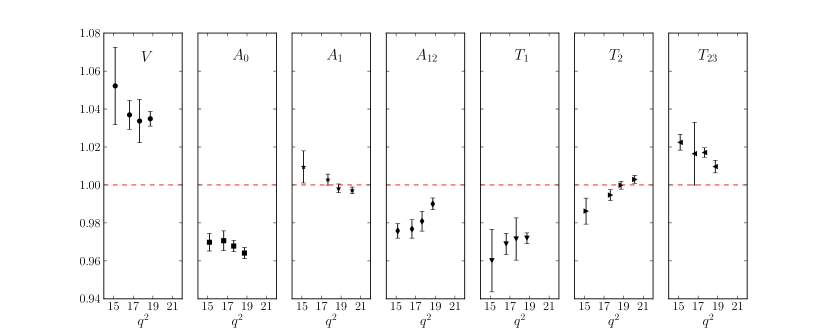
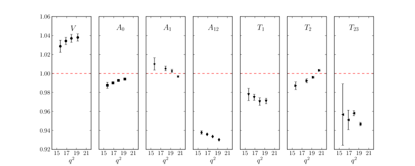
The comparison between the frequentist and Bayesian analyses described above produced results which agree or differ within 1–2 times the statistical and fitting uncertainties. Where such differences appear, it is usually the case that the energies determined by the frequentist fits were about 1$\sigma$ lower than those from the Bayesian fits. This suggests that the Bayesian fits, which were restricted to more limited set of $T$ values, may have been more subject to excited state contamination. Given the flexibility of the frequentist fits to explore a wider variety of fit ranges in Euclidean time we take these as our main results, with the Bayesian fits giving important cross-checks.

In Table 4 we give the meson masses resulting from fits to correlation functions as described above. Where comparisons can be made, these agree with calculations done by other groups on the same lattices with the same parameters Aubin:2004wf . The masses indicate that the valence strange and bottom quark masses are not precisely tuned to their physical values. We estimate the resulting systematic errors in Sec. V.

In Fig. 1 we compare the form factors computed with currents matched at leading order in $\Lambda_{{\scriptscriptstyle\mathrm{QCD}}}/m_{b}$ (LO) to those which include next-to-leading order (NLO) $\Lambda_{{\scriptscriptstyle\mathrm{QCD}}}/m_{b}$-corrections in the currents. (Both LO and NLO form factors are matched at 1-loop in $\alpha_{s}$.) The plots are shown for $B_{s}\to\phi$ decays since the statistical errors are smallest, but the ratios are of comparable size for $B\to K^{*}$ and $B_{s}\to K^{*}$ form factors, namely at most 7% away from unity. The statistical errors in the ratio are very small because the ratio can be taken for each bootstrap sample individually, taking correlations into account. The significance of including NLO operators is reduced when considering the absolute values of the form factors and the results of fits to the form factor shapes as discussed in the next Section. Most results differ at or below the $1\sigma$ statistical-plus-fitting uncertainty. Nevertheless we take the NLO-matched fits as our final results, so the largest terms truncated from the matching are $O(\alpha_{s}^{2},\alpha_{s}\Lambda_{{\scriptscriptstyle\mathrm{QCD}}}/m_{b},(\Lambda_{{\scriptscriptstyle\mathrm{QCD}}}/m_{b})^{2})$.

In the Appendix we provide tables of form factor results on each lattice for several final-state momenta. We also tabulate corresponding values for useful kinematic variables. In general these raw lattice results still need to account for dependence on light quark mass. In the next section we describe our fits to the kinematic shape and quark mass dependence of the lattice data.

IV Form factor shape

Since exclusive semileptonic branching fractions can precisely determine CKM matrix elements, there is a sizeable body of work discussing accurate parametrizations for form factor shapes Bourrely:1980gp ; Boyd:1994tt ; Lellouch:1995yv ; Becirevic:1997vw ; Boyd:1997qw ; Mannel:1998kp ; Becirevic:1999kt ; Flynn:2000gd ; Ball:2004rg ; Hill:2005ju ; Becher:2005bg ; Arnesen:2005ez ; Flynn:2006vr ; Flynn:2007qd ; Bourrely:2008za ; Flynn:2008zr ; Bernard:2009ke ; Bharucha:2010im . The method we use here is based on the simplified series expansion Bourrely:2008za , modified to account for lattice spacing and quark mass dependence Na:2010uf .

Using $t=q^{2}$ and $t_{\pm}=(m_{B_{(s)}}\pm m_{V})^{2}$, one constructs a dimensionless variable which is small,

$$z(t,t_{0})~{}=~{}\frac{\sqrt{t_{+}-t}-\sqrt{t_{+}-t_{0}}}{\sqrt{t_{+}-t}+\sqrt{t_{+}-t_{0}}}\,.$$ (36)

The $t_{0}$ parameter simply shifts the origin and can be chosen to minimize $|z|$ over the $q^{2}$ range of interest. For simplicity we use $t_{0}=12~{}\mathrm{GeV}^{2}$ throughout this paper. One might try to optimize the choice of $t_{0}$ to make the series expansion in $z$ converge most quickly Bharucha:2010im ; however, we see no discernible in our final results if $t_{0}$ is varied by several GeV². After removing any poles due to bound-state resonances, the form factors are represented by a power series in $z$. One can introduce additional coefficients to account for lattice spacing and mass dependence Na:2010uf . Therefore, we fit the form factors $F=V,A_{0},A_{1},A_{12},T_{1},T_{2},T_{23}$ to the following form:

$$F(t)~{}=~{}\frac{1}{P(t;\Delta m)}[1+b_{1}(aE_{F})^{2}+\ldots]\sum_{n}a_{n}d_{n}z^{n}$$ (37)

where the pole factor is given as

$$P(t;\Delta m)~{}=~{}1-\frac{t}{(m_{B_{(s)}}+\Delta m)^{2}}\,.$$ (38)

Changing the numerical value of $t_{0}$ by a few GeV² simply results in a compensating shift in the $a_{n}$, without significantly affecting the values of the fit function $F(t)$.

Table 5: Mass differences (in MeV), between the initial state and pertinent resonance, used in the function $P(t,\Delta m)$.

Form factor	$B\to K^{*}$	$B_{s}\to\phi$	$B_{s}\to K^{*}$
$A_{0}$	87	0	$-87$
$V$, $T_{1}$	135	45	$-42$
$A_{1}$, $A_{12}$, $T_{2}$, $T_{23}$	550	440	350

The mass of the resonance used as input to the fits is taken to be a fixed splitting (in physical units) above the initial state meson $m_{\mathrm{res}}=m_{B_{(s)}}+\Delta m$. The value of $\Delta m$ depends on the lowest lying resonance contributing to a particular form factor. The values we use are given in Table 5. Fits have been redone, varying these $\Delta m$ values by 20% and this has no effect on the final results for the form factor curves (although the fit parameters vary to compensate for the change in $\Delta m$).

The dependence of the form factor on the quark masses is taken into account by the $d_{n}$ terms

$$d_{n}=[1 +c_{n1}\Delta x+c_{n2}(\Delta x)^{2}+\ldots$$

$$+c_{n1s}\Delta x_{s}+c_{n2s}(\Delta x_{s})^{2}+\ldots]$$ (39)

with $\Delta x=(m_{\pi}^{2}-m_{\pi,\mathrm{phys}}^{2})/(4\pi f_{\pi})^{2}$ and $\Delta x_{s}=(m_{\eta_{s}}^{2}-m_{\eta_{s},\mathrm{phys}}^{2})/(4\pi f_{\pi})^{2}$ acting as proxies for the differences away from physical $u/d$ and $s$ quark masses, respectively. We use $f_{\pi}=132~{}\mathrm{MeV}$ and the pseudoscalar meson masses displayed in Table 4.

Our data for the separate $B\to K^{*}$, $B_{s}\to K^{*}$, and $B_{s}\to\phi$ form factors are computed with constant, somewhat mistuned values of the strange quark mass. We can estimate the dependence on the valence strange quark mass by performing a simultaneous fit which treats the $B\to K^{*}$ and $B_{s}\to K^{*}$ form factors as calculations of the $B_{s}\to\phi$ form factors using a very mistuned spectator or offspring quark mass. Departures from the physical strange mass are parametrized in terms of the corresponding pseudoscalar meson mass:

$$\Delta y = \frac{1}{(4\pi f_{\pi})^{2}}\left(m_{\mathrm{offspr}}^{2}-m_{\eta_{s},\mathrm{phys}}^{2}\right)$$

$$\Delta w = \frac{1}{(4\pi f_{\pi})^{2}}\left(m_{\mathrm{spect}}^{2}-m_{\eta_{s},\mathrm{phys}}^{2}\right)\,.$$ (40)

For example, $\Delta y=\Delta w\approx 2\%(4\%)$ for the $B_{s}\to\phi$ form factors on the coarse (fine) lattice. In the case of $B\to K^{*}$ form factors, $\Delta y\approx 2\%(4\%)$ for the coarse (fine) lattice and $\Delta w\approx-8\%$ to $-13\%$ depending on the “light” quark mass. These values are swapped when considering $B_{s}\to K^{*}$ decays.

We obtain good fits to all the data for a particular form factor $F$ using the following ansatz:

$$F(t;\Delta y,\Delta w)\;=\; \frac{1}{P(t)}\left[a_{0}\left(1+f_{01}\Delta y+g_{01}\Delta w\right)+a_{1}z\right]\,.$$ (41)

Results of the fits for the form factors $V$, $A_{0}$, $A_{1}$, $A_{12}$, and $T_{23}$ are given in Table 6. (The tables of fit results also give matrix elements $C(p,q)$ of the correlation matrix. These are related to covariance matrix elements $\sigma(p,q)$ by $C(p,q)=\sigma(p,q)/(\sigma_{p}\sigma_{q})$, with $\sigma(p,p)=\sigma_{p}^{2}$.) Fits were also performed allowing $a_{1}z$ to be multiplied by a factor $(1+f_{11}\Delta y+g_{11}\Delta w)$; however, the data do not constrain the parameters $f_{11}$ and $g_{11}$.

Our final results for the form factors are obtained by separately considering the form factors with specific initial and final state combinations. In each case we use the following function to fit form factor $F(t)$

$$F(t)~{}=~{}\frac{1}{P(t)}[a_{0}(1+c_{01}\Delta x+c_{01s}\Delta x_{s})+a_{1}z]\,.$$ (42)

The parameter describing the strange-quark mass dependence $c_{01s}$ is included in the fit with a Gaussian prior using the results in Table 6: $c_{01s}=f_{01}$ for the $B\to K^{*}$ form factors, $c_{01s}=g_{01}$ for $B_{s}\to K^{*}$, and $c_{01s}=f_{01}+g_{01}$ for $B_{s}\to\phi$. In the last case, the width for the $c_{01s}$ prior is taken by combining the $f_{01}$ and $g_{01}$ uncertainties in quadrature. The parameters $a_{0}$, $a_{1}$, and $c_{01}$ are not constrained by priors. We find the lattice spacing dependence to be negligible when we include the parameter $b_{1}$ in fits of the form (37), therefore we do not include this parameter in our final fits. The results, including correlation matrices, are given in Table 7 for 5 of the $B\to K^{*}$ form factors and Table 8 for 5 of the $B_{s}\to\phi$ form factors. (See the Appendix for $B_{s}\to K^{*}$ form factors.)

We have an extra piece of information about the $T_{1}(q^{2})$ and $T_{2}(q^{2})$ form factors, namely the kinematic constraint that they equal each other at $q^{2}=0$. We implement this by performing a combined eight-parameter fit, with each form factor parametrized as in (42), and adding to the $\chi^{2}$ function a term $[a_{0}^{T_{1}}-a_{0}^{T_{2}}+(a_{1}^{T_{1}}-a_{1}^{T_{2}})z_{0}]^{2}/10^{-8}$, where $z_{0}=z(0,12~{}\mathrm{GeV}^{2})$. As with the other form factors, we first determine the parameters governing the strange-quark mass dependence by a joint fit to $B_{s}\to\phi$, $B\to K^{*}$, and $B_{s}\to K^{*}$ form factors (Table 9). Those parameters are then included in the eight-parameter fit, the results of which appear in Tables 10 and 11 (and the Appendix).

We obtain values for $\chi^{2}$ per degree-of-freedom close to 1 for all the fits to form factor shape. Nevertheless, we have experimented with including terms corresponding to the parameters $c_{11}$ and $c_{02}$, using Gaussian priors to prevent the fits from diverging. As we found with including a $b_{1}$ parameter in the fit, the data clearly do not constrain these parameters. The fit returns a value and error for these parameters corresponding to the prior mean and width, for narrow and wide Gaussians. The $\chi^{2}$ of the fit is unaffected by including or excluding terms in this way.

Table 6: Fit results (with correlation matrices) determining the dependence of form factors on the strange quark mass.

$P(t)V(t)$
$p$	Value	$C(p,a_{0})$	$C(p,a_{1})$	$C(p,f_{01})$
$a_{0}$	$0.5386(196)$
$a_{1}$	$-1.85(35)$	$0.95$
$f_{01}$	$1.069(112)$	$-0.66$	$-0.60$
$g_{01}$	$-0.047(134)$	$-0.34$	$-0.21$	$0.17$
$P(t)A_{0}(t)$
$p$	Value	$C(p,a_{0})$	$C(p,a_{1})$	$C(p,f_{01})$
$a_{0}$	$0.5538(181)$
$a_{1}$	$-1.48(32)$	$0.96$
$f_{01}$	$0.420(80)$	$-0.44$	$-0.41$
$g_{01}$	$-0.163(144)$	$-0.44$	$-0.30$	$0.42$
$P(t)A_{1}(t)$
$p$	Value	$C(p,a_{0})$	$C(p,a_{1})$	$C(p,f_{01})$
$a_{0}$	$0.2984(70)$
$a_{1}$	$0.158(99)$	$0.97$
$f_{01}$	$0.841(52)$	$-0.67$	$-0.65$
$g_{01}$	$-0.053(78)$	$-0.20$	$-0.09$	$0.17$
$P(t)A_{12}(t)$
$p$	Value	$C(p,a_{0})$	$C(p,a_{1})$	$C(p,f_{01})$
$a_{0}$	$0.2057(71)$
$a_{1}$	$0.406(124)$	$0.97$
$f_{01}$	$0.151(91)$	$-0.35$	$-0.36$
$g_{01}$	$-0.599(137)$	$-0.19$	$-0.10$	$0.29$
$P(t)T_{23}(t)$
$p$	Value	$C(p,a_{0})$	$C(p,a_{1})$	$C(p,f_{01})$
$a_{0}$	$0.5167(113)$
$a_{1}$	$0.389(187)$	$0.97$
$f_{01}$	$0.476(44)$	$-0.59$	$-0.62$
$g_{01}$	$-0.321(102)$	$-0.25$	$-0.12$	$0.03$

V Discussion of results and systematic uncertainties

In this section we present our main results and discuss the systematic uncertainties in our calculations of the form factors. We compare our results to other determinations.

The results of the fits for the meson masses in Table 4 indicate that the heavy quark mass has been tuned so that the $B$ and $B_{s}$ masses are 5% too heavy. In the $m_{B}\to\infty$ limit the form factors scale like Isgur:1990kf (also Grinstein:2004vb )

$$V,A_{0},T_{1},T_{23}\propto m_{B}^{1/2}$$

$$A_{1},A_{12},T_{2}\propto m_{B}^{-1/2}\,.$$ (43)

Therefore, we compensate for this error due to the $m_{b}$ mistuning by scaling the central values of the form factors by $0.976$ ($V$, $A_{0}$, $T_{1}$, $T_{23}$) and $1.025$ ($A_{1}$, $A_{12}$, $T_{2}$). The remaining error is suppressed compared to (43) by a factor of $\Lambda_{{\scriptscriptstyle\mathrm{QCD}}}/m_{b}$; i.e. the remaining $m_{b}$ mistuning error is well below 1% and is treated as negligible compared to other uncertainties.

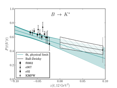
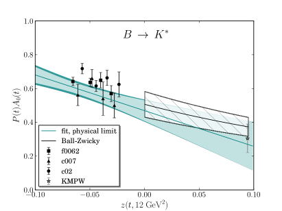
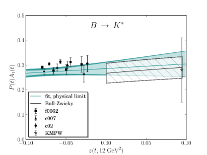
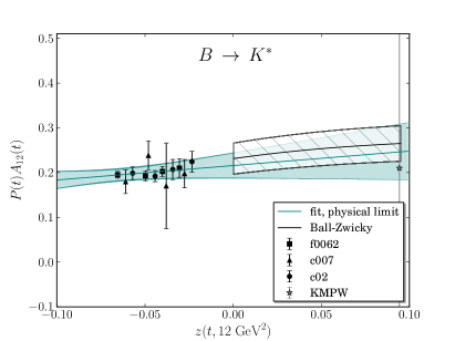
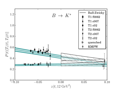
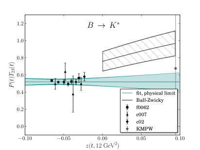
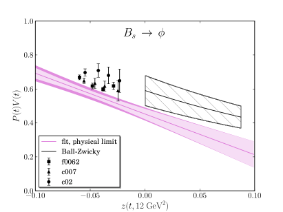
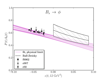
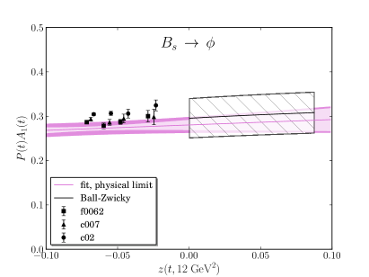
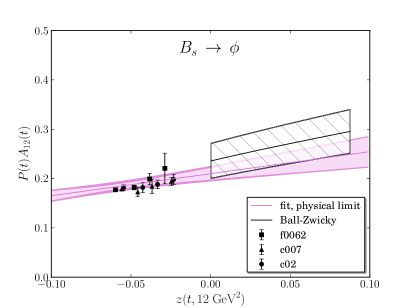
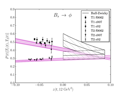
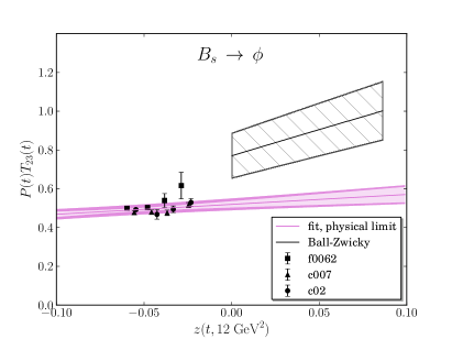
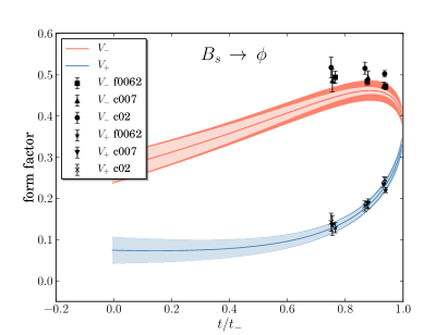
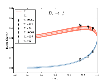
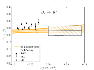
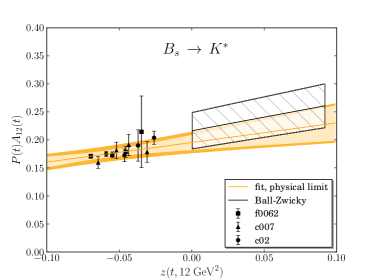
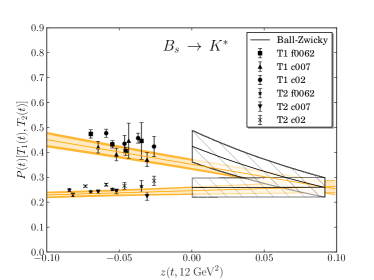
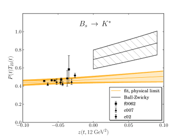
The $B\to K^{*}$, $B_{s}\to\phi$, and $B_{s}\to K^{*}$ form factors have been fit to the form given in Eq. (42). All fits have been done after compensating for the mistuning of the heavy quark mass. The results for $B\to K^{*}$ and $B_{s}\to\phi$ are tabulated in Tables 7–11, along with their correlation matrices. Figures 2 and 3 show the form factor fits, along with the lattice data. These tables and curves constitute our final results. Data points corresponding to the physical limit can be obtained from the fits by setting $\Delta x=0$ and $\Delta x_{s}=0$ in Eq. (42). The corresponding tables and plots for $B_{s}\to K^{*}$ form factors appear in the Appendix. In order to aid comparison with other work, a table in the Appendix gives numerical results for the form factors in the physical limit at a few fiducial values of $q^{2}$.

In Figs. 2 and 3 we also plot results from light-cone sum rules (LCSR) Ball:2004rg with a uniform 15% error band Bobeth:2010wg . There have also been LCSR calculations of the $B\to K^{*}$ form factors using $B$ meson distribution amplitudes Khodjamirian:2010vf ; these are in agreement but quote larger uncertainties so we only display their $q^{2}=0$ points. The agreement between the LQCD and LCSR results is generally good. The $T_{23}$ form factors extracted from Ball and Zwicky are notable exceptions. It is likely that 15% is an underestimate of the LCSR uncertainty in this linear combination of the $T_{2}$ and $\tilde{T}_{3}$ form factors calculated by Ball and Zwicky. We, however, are not in a place to better estimate their uncertainties, so we interpret the 15% error band in our paper in a weaker sense than a $1\sigma$ range. Propagating the uncertainties in $T_{2}$ and $T_{3}$ determined by Khodjamirian et al. as uncorrelated leads to large uncertainties in $T_{23}$, even if the central values are in good agreement with our results. The $V$ form factors for $B_{s}\to\phi$ and $B_{s}\to K^{*}$ also appear to disagree with extrapolations of our lattice data to large recoil. One possibility is that a $z^{2}$ term is necessary to fit both results.

Our extrapolation of $B\to K^{*}$ form factors $T_{1}$ and $T_{2}$ agrees with the latest quenched lattice QCD results for the $q^{2}=0$ value of $T_{1}(0)=T_{2}(0)$ Becirevic:2006nm (see Fig. 2). Form factors have also been predicted using a relativistic quark model Ebert:2010dv ; Faustov:2013pca .

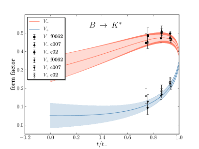
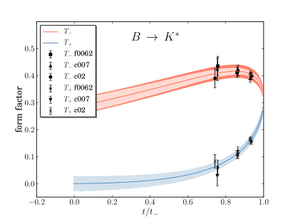
Fig. 4 shows the results for the form factors $V_{\pm}$ and $T_{\pm}$. Note in these cases, the fits are not done directly to the data; instead the curves are the results of linearly combining the fits in Tables 7–11.

Figure 2: $B\to K^{*}$ form factors. Data points for the three ensembles of lattice gauge fields appear in black. The fit of the lattice data to the function of Eq. (42), extrapolated to the physical quark mass limit, is shown as a solid curve, with statistical (pale) and total (dark) error bands. For comparison, the LCSR results of Ball:2004rg are shown with a 15% uncertainty (hatched band) Bobeth:2010wg . We also display $q^{2}=0$ LCSR results from Khodjamirian:2010vf as gray stars (central values shifted slightly so that error bars are symmetric); the errors have been propagated as uncorrelated for $A_{12}$ and $T_{23}$ possibly resulting in overestimates of the corresponding uncertainties. In the lower left plot, the quenched lattice QCD result for $T_{1}(0)=T_{2}(0)$ Becirevic:2006nm is displayed as a gray triangle.

Figure 3: $B_{s}\to\phi$ form factors, as in Fig. 2.

Figure 4: Curves describing helicity basis form factors $V_{\pm}(q^{2})$ and $T_{\pm}(q^{2})$ form factors for $B\to K^{*}$ (top) and $B_{s}\to\phi$ (bottom). Data points represent the linear combinations (13) computed on each ensemble. The curves are obtained by using the fit results in Tables 7–11 in the physical quark mass limit, with statistical (pale) and total (dark) error bands shown.

Table 7: Results and correlation matrices of fits to $B\to K^{*}$ form factors.

$P(t;135\mathrm{MeV})V(t)$
$p$	Value	$C(p,a_{0})$	$C(p,a_{1})$	$C(p,c_{01})$
$a_{0}$	$0.496(67)$
$a_{1}$	$-2.03(92)$	$0.86$
$c_{01}$	$1.38(1.49)$	$-0.79$	$-0.41$
$c_{01s}$	$1.066(112)$	$-0.04$	$-0.00$	$0.02$
$P(t;87\mathrm{MeV})A_{0}(t)$
$p$	Value	$C(p,a_{0})$	$C(p,a_{1})$	$C(p,c_{01})$
$a_{0}$	$0.469(61)$
$a_{1}$	$-2.11(88)$	$0.86$
$c_{01}$	$2.46(1.27)$	$-0.76$	$-0.39$
$c_{01s}$	$0.421(80)$	$-0.02$	$0.00$	$0.02$
$P(t;550\mathrm{MeV})A_{1}(t)$
$p$	Value	$C(p,a_{0})$	$C(p,a_{1})$	$C(p,c_{01})$
$a_{0}$	$0.286(24)$
$a_{1}$	$0.19(28)$	$0.94$
$c_{01}$	$1.07(53)$	$-0.68$	$-0.42$
$c_{01s}$	$0.841(52)$	$-0.02$	$0.01$	$0.02$
$P(t;550\mathrm{MeV})A_{12}(t)$
$p$	Value	$C(p,a_{0})$	$C(p,a_{1})$	$C(p,c_{01})$
$a_{0}$	$0.216(27)$
$a_{1}$	$0.32(38)$	$0.91$
$c_{01}$	$-0.12(97)$	$-0.65$	$-0.33$
$c_{01s}$	$0.151(91)$	$-0.03$	$0.00$	$0.02$
$P(t;550\mathrm{MeV})T_{23}(t)$
$p$	Value	$C(p,a_{0})$	$C(p,a_{1})$	$C(p,c_{01})$
$a_{0}$	$0.520(45)$
$a_{1}$	$-0.00(63)$	$0.84$
$c_{01}$	$-0.07(65)$	$-0.59$	$-0.11$
$c_{01s}$	$0.474(44)$	$-0.02$	$0.00$	$0.02$

Table 8: Results and correlation matrices of fits to $B_{s}\to\phi$ form factors.

$P(t;45\mathrm{MeV})V(t)$
$p$	Value	$C(p,a_{0})$	$C(p,a_{1})$	$C(p,c_{01})$
$a_{0}$	$0.452(30)$
$a_{1}$	$-2.40(50)$	$0.80$
$c_{01}$	$2.80(1.04)$	$-0.69$	$-0.18$
$c_{01s}$	$0.998(175)$	$-0.14$	$-0.03$	$0.07$
$P(t;0\mathrm{MeV})A_{0}(t)$
$p$	Value	$C(p,a_{0})$	$C(p,a_{1})$	$C(p,c_{01})$
$a_{0}$	$0.525(21)$
$a_{1}$	$-1.63(39)$	$0.83$
$c_{01}$	$0.81(52)$	$-0.38$	$0.13$
$c_{01s}$	$0.248(164)$	$-0.13$	$0.04$	$0.06$
$P(t;440\mathrm{MeV})A_{1}(t)$
$p$	Value	$C(p,a_{0})$	$C(p,a_{1})$	$C(p,c_{01})$
$a_{0}$	$0.2803(113)$
$a_{1}$	$0.121(150)$	$0.92$
$c_{01}$	$1.01(29)$	$-0.64$	$-0.33$
$c_{01s}$	$0.768(94)$	$-0.10$	$-0.01$	$0.07$
$P(t;440\mathrm{MeV})A_{12}(t)$
$p$	Value	$C(p,a_{0})$	$C(p,a_{1})$	$C(p,c_{01})$
$a_{0}$	$0.2098(115)$
$a_{1}$	$0.447(186)$	$0.92$
$c_{01}$	$-0.18(41)$	$-0.57$	$-0.25$
$c_{01s}$	$-0.435(163)$	$-0.10$	$0.03$	$0.06$
$P(t;440\mathrm{MeV})T_{23}(t)$
$p$	Value	$C(p,a_{0})$	$C(p,a_{1})$	$C(p,c_{01})$
$a_{0}$	$0.5194(157)$
$a_{1}$	$0.51(25)$	$0.88$
$c_{01}$	$0.02(24)$	$-0.48$	$-0.08$
$c_{01s}$	$0.186(110)$	$-0.13$	$0.03$	$0.10$

Table 9: Fit results (with correlation matrix) determining the dependence of $T_{1}$ and $T_{2}$ form factors on the strange quark mass.

$p$	Value	$C(p,a_{0}^{T_{1}})$	$C(p,a_{1}^{T_{1}})$	$C(p,f_{01}^{T_{1}})$	$C(p,g_{01}^{T_{1}})$	$C(p,a_{0}^{T_{2}})$	$C(p,a_{1}^{T_{2}})$	$C(p,f_{01}^{T_{2}})$
$a_{0}^{T_{1}}$	$0.4434(50)$
$a_{1}^{T_{1}}$	$-1.140(61)$	$0.74$
$f_{01}^{T_{1}}$	$1.224(61)$	$-0.28$	$-0.01$
$g_{01}^{T_{1}}$	$-0.249(85)$	$-0.18$	$0.21$	$0.07$
$a_{0}^{T_{2}}$	$0.3039(43)$	$0.94$	$0.91$	$-0.18$	$0.00$
$a_{1}^{T_{2}}$	$0.390(62)$	$0.91$	$0.95$	$-0.12$	$0.05$	$0.98$
$f_{01}^{T_{2}}$	$0.750(38)$	$-0.49$	$-0.38$	$0.21$	$-0.18$	$-0.49$	$-0.43$
$g_{01}^{T_{2}}$	$-0.093(47)$	$0.04$	$0.12$	$0.13$	$0.35$	$0.04$	$0.13$	$-0.07$

Table 10: Results and correlation matrix of the fit to $B\to K^{*}$ form factors $P(t;135\mathrm{MeV})T_{1}(t)$ and $P(t;550\mathrm{MeV})T_{2}(t)$. The fit implements the constraint that $T_{1}(0)=T_{2}(0)$.

$p$	Value	$C(p,a_{0}^{T_{1}})$	$C(p,a_{1}^{T_{1}})$	$C(p,c_{01}^{T_{1}})$	$C(p,a_{0}^{T_{2}})$	$C(p,a_{1}^{T_{2}})$	$C(p,c_{01}^{T_{2}})$	$C(p,c_{01s}^{T_{1}})$
$a_{0}^{T_{1}}$	$0.422(24)$
$a_{1}^{T_{1}}$	$-1.37(25)$	$0.48$
$c_{01}^{T_{1}}$	$0.71(85)$	$-0.75$	$0.05$
$a_{0}^{T_{2}}$	$0.2830(197)$	$0.86$	$0.81$	$-0.43$
$a_{1}^{T_{2}}$	$0.10(24)$	$0.82$	$0.86$	$-0.37$	$0.91$
$c_{01}^{T_{2}}$	$0.45(46)$	$-0.51$	$-0.32$	$0.39$	$-0.64$	$-0.32$
$c_{01s}^{T_{1}}$	$1.223(61)$	$-0.03$	$0.02$	$0.01$	$-0.01$	$-0.01$	$0.00$
$c_{01s}^{T_{2}}$	$0.750(38)$	$-0.00$	$0.00$	$0.00$	$-0.01$	$0.01$	$0.01$	$0.00$

Table 11: Results and correlation matrix of the fit to $B_{s}\to\phi$ form factors $P(t;45\mathrm{MeV})T_{1}(t)$ and $P(t;440\mathrm{MeV})T_{2}(t)$. The fit implements the constraint that $T_{1}(0)=T_{2}(0)$.

$p$	Value	$C(p,a_{0}^{T_{1}})$	$C(p,a_{1}^{T_{1}})$	$C(p,c_{01}^{T_{1}})$	$C(p,a_{0}^{T_{2}})$	$C(p,a_{1}^{T_{2}})$	$C(p,c_{01}^{T_{2}})$	$C(p,c_{01s}^{T_{1}})$
$a_{0}^{T_{1}}$	$0.4070(104)$
$a_{1}^{T_{1}}$	$-1.093(119)$	$0.22$
$c_{01}^{T_{1}}$	$1.48(59)$	$-0.67$	$0.36$
$a_{0}^{T_{2}}$	$0.2890(81)$	$0.78$	$0.73$	$-0.22$
$a_{1}^{T_{2}}$	$0.265(97)$	$0.74$	$0.78$	$-0.18$	$0.89$
$c_{01}^{T_{2}}$	$0.66(24)$	$-0.48$	$-0.33$	$0.25$	$-0.69$	$-0.33$
$c_{01s}^{T_{1}}$	$0.974(105)$	$-0.12$	$0.06$	$0.02$	$-0.03$	$-0.04$	$0.00$
$c_{01s}^{T_{2}}$	$0.658(48)$	$-0.01$	$-0.02$	$-0.00$	$-0.05$	$0.01$	$0.03$	$0.00$

Table 12: Estimates of systematic uncertainties. Effects due to light quark mass dependence and lattice spacing dependence are included in the statistical fitting uncertainties.

Source	Size
Truncation of $O(\alpha_{s}^{2})$ terms	4%
Truncation of $O(\alpha_{s}\Lambda_{{\scriptscriptstyle\mathrm{QCD}}}/m_{b})$ terms	2%
Truncation of $O(\Lambda_{{\scriptscriptstyle\mathrm{QCD}}}^{2}/m_{b}^{2})$ terms	1%
Mistuning of $m_{b}$	$<1\%$
Net systematic uncertainty	5%

The uncertainties in the fit parameters reflect both statistical fluctuations and effects due to quark mass extrapolation. The inclusion in the fits of a term to account for finite lattice spacing effects had no significant effect on the results. It is evident from the figures that the data from ensemble f0062 and c007 show little systematic difference. Therefore we assume that errors due to discretization are not significant compared to the statistical and fitting uncertainties.

In Table 12 we summarize our estimates for other sources of systematic uncertainties. The largest of these, at 4%, is due to the truncation of $O(\alpha_{s}^{2})$ terms in the perturbative matching from lattice NRQCD to the continuum, as discussed in detail in Sec. III.3.

In the previous section we have already discussed our determination of the strange quark mass dependence of the form factors. Whether or not we interpolate the form factors to the physical strange quark mass we obtain fit results consistent within errors. Since we use the interpolated values, the remaining uncertainty due to mistuned strange quark mass is negligible compared to other sources of uncertainty.

Partial quenching effects due to different sea and valence strange quark masses should also be negligible. This is clear in the pseudoscalar sector where one can use partially quenched chiral perturbation theory to predict the size of such effects; sea quark mass effects arise at one-loop order while valence quark masses affect tree-level diagrams. Given that even the leading order linear mass dependence in the $B\to V$ form factors is barely significant statistically the form factors are assumed to be insensitive to the “loop-suppressed” effects of partial quenching for the strange quark mass.

Our calculation of $B_{s}\to\phi$ form factors neglects disconnected contributions to the $\phi$ propagator. The OZI rule suggests such effects, due to pair annihilation and creation of the valence strange quark–antiquark pair, are small for vector and axial-vector mesons.

Table 13: $B\to K^{*}$ form factor ratios. Statistical uncertainties were determined by bootstrap analysis.

Ensemble	$|{\bf\bm{n}}|^{2}$	$V/A_{1}$	$A_{12}/A_{1}$	$T_{1}/T_{2}$	$T_{23}/T_{2}$
f0062	1	2.83(17)	0.70(4)	2.25(10)	1.89(7)
	2	2.62(19)	0.69(6)	2.13(14)	1.84(12)
	4	2.2(3)	0.69(10)	2.0(2)	1.9(3)
c007	1	2.70(13)	0.62(9)	2.16(12)	1.8(2)
	2	2.74(20)	0.79(11)	2.13(17)	2.2(3)
	4	2.5(4)	0.75(16)	2.2(4)	1.9(3)
c02	1	2.57(13)	0.64(4)	2.16(11)	1.73(5)
	2	2.4(3)	0.62(5)	2.03(14)	1.67(13)
	4	1.8(4)	0.73(11)	1.7(3)	2.0(2)

Table 14: $B_{s}\to\phi$ form factor ratios. Statistical uncertainties were determined by bootstrap analysis.

Ensemble	$|{\bf\bm{n}}|^{2}$	$V/A_{1}$	$A_{12}/A_{1}$	$T_{1}/T_{2}$	$T_{23}/T_{2}$
f0062	1	2.83(7)	0.635(18)	2.23(7)	1.77(4)
	2	2.49(9)	0.636(19)	1.96(6)	1.74(3)
	4	2.28(12)	0.73(10)	1.80(8)	2.0(3)
c007	1	2.67(7)	0.627(19)	2.10(5)	1.72(4)
	2	2.48(12)	0.59(3)	1.97(11)	1.69(4)
	4	2.2(3)	0.65(5)	1.61(19)	1.80(11)
c02	1	2.67(8)	0.597(18)	2.11(8)	1.69(2)
	2	2.65(16)	0.60(3)	2.06(11)	1.61(9)
	4	2.2(2)	0.62(3)	1.76(15)	1.68(8)

Table 15: Fit results and correlation matrices determining dependence of form factor ratios on strange quark mass.

$V/A_{1}\times P(t,\Delta m_{V})/P(t,\Delta m_{A_{1}})$
$p$	Value	$C(p,a_{0})$	$C(p,a_{1})$	$C(p,f_{01})$
$a_{0}$	$1.679(97)$
$a_{1}$	$-10.38(1.73)$	$0.96$
$f_{01}$	$0.321(172)$	$-0.16$	$-0.16$
$g_{01}$	$0.31(23)$	$-0.11$	$-0.00$	$0.13$
$A_{12}/A_{1}$
$p$	Value	$C(p,a_{0})$	$C(p,a_{1})$	$C(p,f_{01})$
$a_{0}$	$0.687(39)$
$a_{1}$	$0.92(68)$	$0.98$
$f_{01}$	$-0.590(133)$	$-0.09$	$-0.10$
$g_{01}$	$-0.41(22)$	$-0.11$	$-0.03$	$0.24$
$T_{1}/T_{2}\times P(t,\Delta m_{T_{1}})/P(t,\Delta m_{T_{2}})$
$p$	Value	$C(p,a_{0})$	$C(p,a_{1})$	$C(p,f_{01})$
$a_{0}$	$1.4847(128)$
$a_{1}$	$-5.315(141)$	$-1.00$
$f_{01}$	$0.230(145)$	$0.18$	$-0.18$
$g_{01}$	$-0.232(198)$	$-0.09$	$0.09$	$0.07$
$T_{23}/T_{2}$
$p$	Value	$C(p,a_{0})$	$C(p,a_{1})$	$C(p,f_{01})$
$a_{0}$	$1.650(75)$
$a_{1}$	$-1.75(1.36)$	$0.98$
$f_{01}$	$-0.264(79)$	$-0.43$	$-0.40$
$g_{01}$	$-0.244(163)$	$-0.16$	$-0.05$	$0.29$

Table 16: Results and correlation matrices of fits to $B\to K^{*}$ form factor ratios. The fit of $T_{1}/T_{2}$ has been constrained to enforce $T_{1}(0)/T_{2}(0)=1$.

$V/A_{1}\times P(t,135\mathrm{MeV})/P(t,550\mathrm{MeV})$
$p$	Value	$C(p,a_{0})$	$C(p,a_{1})$	$C(p,c_{01})$
$a_{0}$	$1.89(28)$
$a_{1}$	$-8.7(4.4)$	$0.83$
$c_{01}$	$-1.33(1.23)$	$-0.35$	$0.18$
$c_{01s}$	$0.321(172)$	$-0.04$	$-0.00$	$0.01$
$A_{12}/A_{1}$
$p$	Value	$C(p,a_{0})$	$C(p,a_{1})$	$C(p,c_{01})$
$a_{0}$	$0.848(154)$
$a_{1}$	$1.5(2.2)$	$0.93$
$c_{01}$	$-1.59(87)$	$-0.46$	$-0.14$
$c_{01s}$	$-0.589(133)$	$-0.02$	$0.01$	$0.02$
$T_{1}/T_{2}\times P(t,135\mathrm{MeV})/P(t,550\mathrm{MeV})$
$p$	Value	$C(p,a_{0})$	$C(p,a_{1})$	$C(p,c_{01})$
$a_{0}$	$1.530(52)$
$a_{1}$	$-5.62(55)$	$-1.00$
$c_{01}$	$-0.18(87)$	$-0.82$	$0.82$
$c_{01s}$	$0.231(145)$	$-0.09$	$0.09$	$0.01$
$T_{23}/T_{2}$
$p$	Value	$C(p,a_{0})$	$C(p,a_{1})$	$C(p,c_{01})$
$a_{0}$	$2.15(26)$
$a_{1}$	$1.9(3.8)$	$0.93$
$c_{01}$	$-1.52(49)$	$-0.36$	$-0.03$
$c_{01s}$	$-0.263(198)$	$-0.06$	$0.02$	$0.07$

Table 17: Results and correlation matrices fits to $B_{s}\to\phi$ form factor ratios. The fit of $T_{1}/T_{2}$ has been constrained to enforce $T_{1}(0)/T_{2}(0)=1$.

$V/A_{1}\times P(t,45\mathrm{MeV})/P(t,440\mathrm{MeV})$
$p$	Value	$C(p,a_{0})$	$C(p,a_{1})$	$C(p,c_{01})$
$a_{0}$	$1.646(165)$
$a_{1}$	$-10.7(2.6)$	$0.90$
$c_{01}$	$0.34(82)$	$-0.53$	$-0.16$
$c_{01s}$	$0.64(29)$	$-0.10$	$0.01$	$0.05$
$A_{12}/A_{1}$
$p$	Value	$C(p,a_{0})$	$C(p,a_{1})$	$C(p,c_{01})$
$a_{0}$	$0.683(54)$
$a_{1}$	$0.26(87)$	$0.92$
$c_{01}$	$-0.86(49)$	$-0.38$	$-0.04$
$c_{01s}$	$-0.91(25)$	$-0.07$	$0.05$	$0.05$
$T_{1}/T_{2}\times P(t,45\mathrm{MeV})/P(t,440\mathrm{MeV})$
$p$	Value	$C(p,a_{0})$	$C(p,a_{1})$	$C(p,c_{01})$
$a_{0}$	$1.472(34)$
$a_{1}$	$-5.43(39)$	$-1.00$
$c_{01}$	$0.15(66)$	$-0.85$	$0.85$
$c_{01s}$	$-0.01(24)$	$-0.24$	$0.24$	$0.05$
$T_{23}/T_{2}$
$p$	Value	$C(p,a_{0})$	$C(p,a_{1})$	$C(p,c_{01})$
$a_{0}$	$1.730(95)$
$a_{1}$	$-1.26(1.68)$	$0.92$
$c_{01}$	$-0.56(33)$	$-0.25$	$0.11$
$c_{01s}$	$-0.448(178)$	$-0.08$	$0.05$	$0.09$

Table 18: Form factors ratios subject to Isgur-Wise relations.

		$B\to K^{*}$		$B_{s}\to\phi$
Ensemble	$|{\bf\bm{n}}|^{2}$	$V/T_{1}$	$A_{1}/T_{2}$	$V/T_{1}$	$A_{1}/T_{2}$
f0062	0	$\cdots$	0.999(12)	$\cdots$	0.994(10)
	1	1.25(5)	0.99(3)	1.26(2)	0.988(17)
	2	1.22(5)	0.99(6)	1.26(4)	0.991(17)
	3	1.21(4)	$\cdots$	1.23(2)	$\cdots$
	4	1.12(11)	1.01(7)	1.25(7)	0.99(3)
c007	0	$\cdots$	0.97(5)	$\cdots$	1.051(10)
	1	1.30(4)	1.04(4)	1.318(19)	1.036(15)
	2	1.34(10)	1.04(3)	1.31(5)	1.040(18)
	3	1.33(9)	$\cdots$	1.34(5)	$\cdots$
	4	1.12(20)	0.98(5)	1.42(16)	1.04(4)
c02	0	$\cdots$	1.046(15)	$\cdots$	1.044(9)
	1	1.24(8)	1.04(3)	1.33(6)	1.046(11)
	2	1.22(9)	1.03(5)	1.34(9)	1.04(3)
	3	1.25(10)	$\cdots$	1.32(10)	$\cdots$
	4	1.10(17)	1.03(9)	1.29(12)	1.02(3)

One question is still left to be addressed: are there any significant quark mass-dependent effects in the form factors as the quark masses are tuned to their physical values so that the vector mesons become unstable in the lattice calculations? In the case which can be studied in heavy-meson chiral perturbation theory, the $B\to D^{*}$ form factor at zero recoil $h_{A_{1}}(1)$, one finds a cusp at the quark mass corresponding to the $D\pi$ threshold which is about a 2% effect Randall:1993qg ; Hashimoto:2001nb ; the cusp is even smaller taking into account staggered quark effects Laiho:2005ue .

Of course this observation does not constitute a reliable estimate of the systematic uncertainty due to $K\pi$ or $KK$ thresholds. However, we do note that the form factors, extrapolated to low $q^{2}$, generally agree with determinations from light-cone sum rules which have systematic errors of a different nature. Given that the $\phi$ is relatively narrow compared to the $K^{*}$, one might expect the threshold effects to be smaller for $B_{s}\to\phi$ form factors than for $B_{(s)}\to K^{*}$. In order to make progress, more theoretical work is necessary to understand how to use LQCD to compute matrix elements involving unstable resonances.

In some phenomenological studies ratios of form factors have been used or extracted from data Hambrock:2012dg ; Hambrock:2013zya . Here we provide tables of the lattice data and simplified series expansion fits directly to several ratios, so that correlations may properly be taken into account. For the ratios, the fit function is simply generalized from (42) in order to take into account the poles in both numerator and denominator:

$$\frac{F_{1}(t)}{F_{2}(t)}~{}=~{}\frac{P_{2}(t)}{P_{1}(t)}[a_{0}(1+c_{01}\Delta x+c_{01s}\Delta x_{s})+a_{1}z]\,.$$ (44)

Monte Carlo data for form factor ratios are given in Tables 13 and 14 for $B\to K^{*}$ and $B_{s}\to\phi$, respectively. The fit results describing the dependence on the strange quark mass appear in Table 15. The fits to the shapes of the form factor ratios are given in Tables 16 and 17 for $B\to K^{*}$ and $B_{s}\to\phi$, respectively.

VI Remarks and conclusions

As Figs. 2 and 3 show, the form factors calculated from lattice QCD at low recoil appear broadly consistent with light cone sum rule determinations at large recoil. The fits to the lattice data included only constant and linear terms in $z$, after removing the pole factor. The presence of a $z^{2}$ term, not necessary to fit the lattice data, would affect the extrapolation of lattice results to low $q^{2}$. One possibility would be to fit both lattice and sum rule results to obtain a parametrization of the form factors over the whole physical range of $q^{2}$ (e.g. as in Ref. Bharucha:2010im ). However, given that short-distance physics can only be isolated well away from sharp resonances $q^{2}<m_{J/\psi}^{2}$ and $q^{2}>m_{\psi^{\prime}}^{2}$ one might choose to use the lattice results for low recoil observables and sum rule results for large recoil observables. If it is possible to obtain precise data in the range $m_{J/\psi}^{2}<q^{2}<m_{\psi^{\prime}}^{2}$, well separated from the resonances, then a combination of lattice and sum rule results would be well motivated.

In addition to providing results useful as inputs to Standard Model (or BSM) predictions for observables, we can consider ratios of form factors which test the accuracy of the heavy quark expansion. To leading order in $\Lambda_{{\scriptscriptstyle\mathrm{QCD}}}/m_{b}$, the one-loop improved Isgur-Wise relations Isgur:1990kf are

$$\frac{V}{T_{1}}\;=\;\kappa~{}~{}~{}\mbox{and}~{}~{}~{}\frac{A_{1}}{T_{2}}\;=\;\kappa\,,$$ (45)

where Grinstein:2004vb ; Bobeth:2010wg

$$\kappa\;=\;1\;-\;\frac{2\alpha_{s}}{3\pi}\,\log\frac{\mu}{m_{b}}\,.$$ (46)

In our calculation, the tensor form factors are quoted with $\mu=m_{b}$. The lattice data for these ratios are tabulated in Table 18. We note that the $O(\Lambda_{{\scriptscriptstyle\mathrm{QCD}}}/m_{b})$ corrections to (45) are rather large for $V/T_{1}$ at about 25%, while significantly smaller for $A_{1}/T_{2}$, less than 10%.

The calculations presented in this paper improve on what is known about the $B\to V$ form factors, especially at large $q^{2}$, which corresponds to the kinematic range accessible on the lattice. Effects of dynamical up, down, and strange quarks are included, allowing us to move beyond the previous quenched determinations of the $B\to V$ form factors. These earlier studies also extrapolated results in heavy quark mass from charm-scale simulations, while NRQCD permits us to calculate form factors directly in the bottom quark sector with presently accessible lattice spacings. We performed a high-statistics study in order to combat the poorer signal-to-noise effects present with vector meson correlation functions. In order to improve upon our calculation, the uncertainty due to the current matching must be reduced, and calculations with lighter quark masses and a finer lattice spacing should be done.

The implications of the lattice QCD calculations presented here are the subject for another paper Horgan:2013pva . There we present results for $B\to K^{*}\mu^{+}\mu^{-}$ and $B_{s}\to\phi\mu^{+}\mu^{-}$ observables at low recoil, both for the Standard Model and beyond. It may be interesting to combine results from lattice and light cone sum rules in order to determine the form factors over the whole kinematic range. Whether this would aid the search for BSM effects in rare $b$ decays remains to be seen.

APPENDIX: DATA TABLES AND $B_{s}\to K^{*}$ FORM FACTORS

Table 19: Form factors parametrizing $B\to K^{*}$ vector and axial-vector matrix elements.

Ensemble	$|{\bf\bm{n}}|^{2}$	$V$	$A_{0}$	$A_{1}$	$A_{12}$
f0062	0	$\cdots$	$\cdots$	0.647(13)	$\cdots$
	1	1.61(6)	1.60(6)	0.57(3)	0.399(15)
	2	1.40(5)	1.44(5)	0.53(4)	0.37(2)
	3	1.23(7)	1.36(9)	$\cdots$	0.37(2)
	4	1.13(14)	1.10(9)	0.52(5)	0.36(3)
c007	0	$\cdots$	$\cdots$	0.61(2)	$\cdots$
	1	1.59(8)	1.38(15)	0.59(3)	0.36(5)
	2	1.55(12)	1.48(12)	0.57(3)	0.45(6)
	3	1.51(13)	1.1(2)	$\cdots$	0.31(17)
	4	1.16(17)	0.99(14)	0.46(5)	0.34(5)
c02	0	$\cdots$	$\cdots$	0.653(12)	$\cdots$
	1	1.60(8)	1.72(7)	0.622(18)	0.40(3)
	2	1.39(13)	1.36(7)	0.58(3)	0.36(2)
	3	1.27(8)	1.34(8)	$\cdots$	0.36(4)
	4	0.92(18)	1.17(13)	0.51(5)	0.37(4)

Table 20: Form factors parametrizing $B\to K^{*}$ tensor matrix elements.

Ensemble	$|{\bf\bm{n}}|^{2}$	$T_{1}$	$T_{2}$	$T_{23}$
f0062	0	$\cdots$	0.648(14)	$\cdots$
	1	1.29(5)	0.58(2)	1.09(3)
	2	1.15(5)	0.54(3)	0.99(5)
	3	1.02(5)	$\cdots$	0.94(5)
	4	1.00(9)	0.51(5)	0.96(8)
c007	0	$\cdots$	0.63(4)	$\cdots$
	1	1.23(6)	0.57(2)	1.01(13)
	2	1.16(9)	0.55(2)	1.21(19)
	3	1.14(9)	$\cdots$	0.7(4)
	4	1.05(17)	0.47(5)	0.86(13)
c02	0	$\cdots$	0.624(14)	$\cdots$
	1	1.29(6)	0.596(15)	1.03(2)
	2	1.14(6)	0.56(3)	0.93(4)
	3	1.01(6)	$\cdots$	0.91(5)
	4	0.82(13)	0.49(4)	0.96(7)

Table 21: Kinematic variables for $B\to K^{*}$ form factor calculations.

Ensemble	$|{\bf\bm{n}}|^{2}$	$E_{K^{*}}(\mathrm{GeV})$	$q^{2}(\mathrm{GeV}^{2})$	$z(q^{2},12~{}\mathrm{GeV}^{2})$
f0062	0	1.033(6)	20.66(5)	$-0.0795(7)$
	1	1.151(10)	19.33(10)	$-0.0655(10)$
	2	1.302(10)	17.73(9)	$-0.0497(9)$
	3	1.391(13)	16.71(11)	$-0.0401(10)$
	4	1.49(2)	15.64(17)	$-0.0305(15)$
c007	0	1.031(9)	20.37(8)	$-0.0773(10)$
	1	1.176(11)	18.81(9)	$-0.0610(10)$
	2	1.296(18)	17.50(15)	$-0.0481(14)$
	3	1.391(18)	16.43(14)	$-0.0380(14)$
	4	1.50(3)	15.3(2)	$-0.0276(19)$
c02	0	1.103(5)	20.12(4)	$-0.0709(5)$
	1	1.234(13)	18.70(9)	$-0.0570(9)$
	2	1.362(13)	17.33(10)	$-0.0443(10)$
	3	1.465(15)	16.21(12)	$-0.0342(9)$
	4	1.59(2)	14.93(18)	$-0.0234(15)$

In Tables 19 and 20 we give the $B\to K^{*}$ form factors computed on each lattice ensemble. For each ensemble, as listed in Table 1, we compute matrix elements with the $K^{*}$ momentum equal to ${\bf\bm{k}}=2\pi{\bf\bm{n}}/aN_{x}$, with ${\bf\bm{n}}=(0,0,0)$, $(1,0,0)$, $(1,1,0)$, $(1,1,1)$, $(2,0,0)$ and their rotational equivalents. There are some blank entries in the tables: in our scheme for extracting the form factors from Eq. (20)–(26), some form factors cannot be extracted when ${\bf\bm{k}}=0$, and $A_{1}$ and $T_{2}$ cannot be isolated without having some component of ${\bf\bm{k}}$ equal to 0. For reference, in Table 21 we also provide the $K^{*}$ energies, $q^{2}$ values, and the numerical value for $z(q^{2},t_{0}=12~{}\mathrm{GeV}^{2})$. Tables 22 and 23 give the lattice results for the $B_{s}\to\phi$ form factors, and Table 24 give the kinematic values.

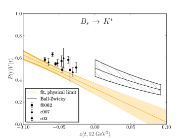
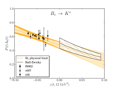
The decay $B_{s}\to K^{*}\ell\nu$ occurs at tree level in the Standard Model, so its precise measurement and comparison to the Standard Model is less likely to reveal physics beyond the Standard Model. In fact the $B_{s}\to K^{*}$ form factors may become useful in future analyses of $b\to d$ decays using the mode $B_{s}\to\bar{K}^{*0}\ell^{+}\ell^{-}$. We have calculated the same set of form factors for $B_{s}\to K^{*}$ exactly in the manner described for $B\to K^{*}$ and $B_{s}\to\phi$ in the main body of the paper, simply by changing the quark masses appropriately. In Table 25 we give the data obtained for the $B_{s}\to K^{*}$ form factors for vector and axial-vector matrix elements. We also give the tensor-current form factor data in Table 26. The data and corresponding fits are shown in Fig. 5. For reference, we also provide a table of the kinematic variables used in the fits (Table 27) and a table of the $B_{s}\to K^{*}$ form factor ratio data (Table 28). Tables 29 and 30 give the final fit parameters and correlation matrices for the seven $B_{s}\to K^{*}$ form factors.

Table 22: Form factors parametrizing $B_{s}\to\phi$ vector and axial-vector matrix elements.

Ensemble	$|{\bf\bm{n}}|^{2}$	$V$	$A_{0}$	$A_{1}$	$A_{12}$
f0062	0	$\cdots$	$\cdots$	0.638(7)	$\cdots$
	1	1.63(3)	1.61(2)	0.577(13)	0.367(8)
	2	1.38(4)	1.411(19)	0.555(10)	0.353(9)
	3	1.24(2)	1.29(2)	$\cdots$	0.36(2)
	4	1.18(4)	1.21(7)	0.519(19)	0.38(5)
c007	0	$\cdots$	$\cdots$	0.649(8)	$\cdots$
	1	1.57(3)	1.57(3)	0.588(12)	0.369(11)
	2	1.41(7)	1.40(3)	0.567(18)	0.332(18)
	3	1.28(6)	1.29(5)	$\cdots$	0.34(3)
	4	1.14(12)	1.14(4)	0.51(3)	0.335(14)
c02	0	$\cdots$	$\cdots$	0.666(7)	$\cdots$
	1	1.66(5)	1.63(4)	0.622(10)	0.371(11)
	2	1.54(9)	1.45(10)	0.578(19)	0.35(2)
	3	1.37(10)	1.24(4)	$\cdots$	0.337(16)
	4	1.21(13)	1.15(8)	0.55(2)	0.337(17)

Table 23: Form factors parametrizing $B_{s}\to\phi$ tensor matrix elements.

Ensemble	$|{\bf\bm{n}}|^{2}$	$T_{1}$	$T_{2}$	$T_{23}$
f0062	0	$\cdots$	0.642(8)	$\cdots$
	1	1.30(3)	0.584(12)	1.032(8)
	2	1.10(3)	0.560(9)	0.976(10)
	3	1.01(2)	$\cdots$	0.98(6)
	4	0.95(4)	0.526(17)	1.06(12)
c007	0	$\cdots$	0.617(8)	$\cdots$
	1	1.19(3)	0.568(13)	0.980(15)
	2	1.07(5)	0.544(13)	0.922(20)
	3	0.95(5)	$\cdots$	0.87(2)
	4	0.79(9)	0.49(3)	0.89(2)
c02	0	$\cdots$	0.638(6)	$\cdots$
	1	1.26(5)	0.595(8)	1.007(11)
	2	1.14(6)	0.556(16)	0.90(5)
	3	1.03(5)	$\cdots$	0.88(3)
	4	0.94(8)	0.534(19)	0.90(3)

Table 24: Kinematic variables for $B_{s}\to\phi$ form factor calculations.

Ensemble	$|{\bf\bm{n}}|^{2}$	$E_{\phi}(\mathrm{GeV})$	$q^{2}(\mathrm{GeV}^{2})$	$z(q^{2},12~{}\mathrm{GeV}^{2})$
f0062	0	1.133(3)	20.52(3)	$-0.0716(3)$
	1	1.242(5)	19.28(4)	$-0.0598(4)$
	2	1.360(6)	17.98(6)	$-0.0480(5)$
	3	1.459(5)	16.86(5)	$-0.0383(4)$
	4	1.565(14)	15.72(11)	$-0.0287(9)$
c007	0	1.137(5)	20.13(5)	$-0.0688(6)$
	1	1.263(4)	18.74(4)	$-0.0556(4)$
	2	1.358(13)	17.65(11)	$-0.0457(10)$
	3	1.448(18)	16.62(15)	$-0.0368(13)$
	4	1.591(14)	15.17(11)	$-0.0246(9)$
c02	0	1.161(5)	20.02(4)	$-0.0667(4)$
	1	1.276(6)	18.73(5)	$-0.0547(5)$
	2	1.403(10)	17.36(8)	$-0.0426(8)$
	3	1.501(6)	16.27(5)	$-0.0333(4)$
	4	1.620(14)	15.03(11)	$-0.0232(9)$

Table 25: Form factors parametrizing $B_{s}\to K^{*}$ vector and axial-vector matrix elements.

Ensemble	$|{\bf\bm{n}}|^{2}$	$V$	$A_{0}$	$A_{1}$	$A_{12}$
f0062	0	$\cdots$	$\cdots$	0.609(14)	$\cdots$
	1	1.59(6)	1.80(6)	0.538(12)	0.382(8)
	2	1.32(4)	1.52(3)	0.510(10)	0.356(11)
	3	1.10(5)	1.32(5)	$\cdots$	0.346(19)
	4	1.0(2)	1.2(3)	0.48(4)	0.39(12)
c007	0	$\cdots$	$\cdots$	0.598(16)	$\cdots$
	1	1.50(8)	1.66(9)	0.558(16)	0.35(2)
	2	1.34(7)	1.50(6)	0.51(2)	0.37(3)
	3	1.33(19)	1.48(10)	$\cdots$	0.37(4)
	4	0.99(8)	1.03(6)	0.43(3)	0.33(3)
c02	0	$\cdots$	$\cdots$	0.649(12)	$\cdots$
	1	1.64(4)	1.66(5)	0.605(11)	0.378(10)
	2	1.35(11)	1.52(14)	0.54(2)	0.35(2)
	3	1.24(6)	1.26(7)	$\cdots$	0.35(5)
	4	1.01(9)	1.22(15)	0.51(3)	0.359(20)

Table 26: Form factors parametrizing $B_{s}\to K^{*}$ tensor matrix elements.

Ensemble	$|{\bf\bm{n}}|^{2}$	$T_{1}$	$T_{2}$	$T_{23}$
f0062	0	$\cdots$	0.611(14)	$\cdots$
	1	1.29(4)	0.541(11)	1.017(11)
	2	1.05(4)	0.514(11)	0.946(14)
	3	0.91(4)	$\cdots$	0.91(3)
	4	0.89(15)	0.48(4)	1.1(3)
c007	0	$\cdots$	0.560(15)	$\cdots$
	1	1.12(7)	0.531(15)	0.93(3)
	2	0.95(6)	0.498(18)	0.92(6)
	3	0.99(15)	$\cdots$	0.82(4)
	4	0.77(6)	0.41(3)	0.82(5)
c02	0	$\cdots$	0.619(10)	$\cdots$
	1	1.24(4)	0.577(11)	1.004(17)
	2	1.03(7)	0.52(3)	0.89(5)
	3	0.97(4)	$\cdots$	0.90(16)
	4	0.84(8)	0.50(3)	0.91(4)

Table 27: Kinematic variables for $B_{s}\to K^{*}$ form factor calculations.

Ensemble	$|{\bf\bm{n}}|^{2}$	$E_{K^{*}}$ (GeV)	$q^{2}$ (GeV2)	$z(q^{2},12\mathrm{GeV}^{2})$
f0062	0	1.034(4)	21.44(4)	$-0.0844(5)$
	1	1.161(8)	20.00(7)	$-0.0696(7)$
	2	1.302(9)	18.47(7)	$-0.0548(7)$
	3	1.385(14)	17.47(12)	$-0.0455(11)$
	4	1.50(3)	16.3(3)	$-0.035(3)$
c007	0	1.031(7)	21.10(7)	$-0.0820(9)$
	1	1.189(7)	19.40(6)	$-0.0646(8)$
	2	1.306(12)	18.09(11)	$-0.0519(11)$
	3	1.38(3)	17.2(3)	$-0.043(3)$
	4	1.518(14)	15.77(12)	$-0.0308(11)$
c02	0	1.106(5)	20.52(5)	$-0.0733(6)$
	1	1.241(5)	19.04(5)	$-0.0590(5)$
	2	1.367(8)	17.66(7)	$-0.0464(6)$
	3	1.461(11)	16.60(8)	$-0.0370(7)$
	4	1.59(2)	15.31(16)	$-0.0260(14)$

Table 28: $B_{s}\to K^{*}$ form factor ratios. Statistical uncertainties were determined by bootstrap analysis.

Ensemble	$|{\bf\bm{n}}|^{2}$	$V/A_{1}$	$A_{12}/A_{1}$	$T_{1}/T_{2}$	$T_{23}/T_{2}$
f0062	1	2.96(11)	0.71(2)	2.39(11)	1.88(4)
	2	2.60(9)	0.70(3)	2.04(8)	1.84(4)
	4	2.1(4)	0.8(2)	1.9(4)	2.2(6)
c007	1	2.69(16)	0.63(4)	2.12(10)	1.75(7)
	2	2.62(16)	0.73(7)	1.90(13)	1.85(14)
	4	2.3(2)	0.76(9)	1.89(14)	2.01(20)
c02	1	2.71(8)	0.625(16)	2.15(7)	1.74(3)
	2	2.49(20)	0.64(5)	1.96(15)	1.69(11)
	4	2.0(2)	0.71(6)	1.68(14)	1.83(14)

Table 29: Results and correlation matrices of fits to $B_{s}\to K^{*}$ form factors.

$P(t;-42\mathrm{MeV})V(t)$
$p$	Value	$C(p,a_{0})$	$C(p,a_{1})$	$C(p,c_{01})$
$a_{0}$	$0.322(48)$
$a_{1}$	$-3.04(67)$	$0.91$
$c_{01}$	$4.82(1.66)$	$-0.87$	$-0.62$
$c_{01s}$	$-0.052(134)$	$-0.04$	$-0.00$	$0.04$
$P(t;-87\mathrm{MeV})A_{0}(t)$
$p$	Value	$C(p,a_{0})$	$C(p,a_{1})$	$C(p,c_{01})$
$a_{0}$	$0.476(42)$
$a_{1}$	$-2.29(74)$	$0.92$
$c_{01}$	$0.46(68)$	$-0.31$	$0.03$
$c_{01s}$	$-0.157(144)$	$-0.06$	$0.01$	$0.05$
$P(t;350\mathrm{MeV})A_{1}(t)$
$p$	Value	$C(p,a_{0})$	$C(p,a_{1})$	$C(p,c_{01})$
$a_{0}$	$0.2342(122)$
$a_{1}$	$0.100(174)$	$0.90$
$c_{01}$	$2.38(48)$	$-0.75$	$-0.44$
$c_{01s}$	$-0.056(78)$	$-0.06$	$0.00$	$0.05$
$P(t;350\mathrm{MeV})A_{12}(t)$
$p$	Value	$C(p,a_{0})$	$C(p,a_{1})$	$C(p,c_{01})$
$a_{0}$	$0.1954(133)$
$a_{1}$	$0.350(190)$	$0.89$
$c_{01}$	$0.19(49)$	$-0.53$	$-0.12$
$c_{01s}$	$-0.590(137)$	$-0.06$	$0.03$	$0.06$
$P(t;350\mathrm{MeV})T_{23}(t)$
$p$	Value	$C(p,a_{0})$	$C(p,a_{1})$	$C(p,c_{01})$
$a_{0}$	$0.472(24)$
$a_{1}$	$0.35(31)$	$0.89$
$c_{01}$	$0.47(42)$	$-0.61$	$-0.23$
$c_{01s}$	$-0.306(102)$	$-0.06$	$0.03$	$0.06$

Table 30: Results and correlation matrix of the fit to $B_{s}\to K^{*}$ form factors $P(t;-42\mathrm{MeV})T_{1}(t)$ and $P(t;440\mathrm{MeV})T_{2}(t)$. The fit implements the constraint that $T_{1}(0)=T_{2}(0)$.

$p$	Value	$C(p,a_{0}^{T_{1}})$	$C(p,a_{1}^{T_{1}})$	$C(p,c_{01}^{T_{1}})$	$C(p,a_{0}^{T_{2}})$	$C(p,a_{1}^{T_{2}})$	$C(p,c_{01}^{T_{2}})$	$C(p,c_{01s}^{T_{1}})$
$a_{0}^{T_{1}}$	$0.3519(137)$
$a_{1}^{T_{1}}$	$-0.992(168)$	$0.09$
$c_{01}^{T_{1}}$	$2.06(73)$	$-0.74$	$0.42$
$a_{0}^{T_{2}}$	$0.2460(108)$	$0.71$	$0.72$	$-0.20$
$a_{1}^{T_{2}}$	$0.169(124)$	$0.65$	$0.78$	$-0.14$	$0.88$
$c_{01}^{T_{2}}$	$1.46(37)$	$-0.51$	$-0.30$	$0.27$	$-0.71$	$-0.34$
$c_{01s}^{T_{1}}$	$-0.248(85)$	$-0.06$	$0.05$	$0.03$	$-0.00$	$-0.00$	$0.00$
$c_{01s}^{T_{2}}$	$-0.093(47)$	$-0.01$	$-0.01$	$0.01$	$-0.03$	$0.01$	$0.03$	$0.00$

Figure 5: $B_{s}\to K^{*}$ form factors, as in Fig. 2.

Finally, in order to facilitate comparison between our results and others, we provide final results for the form factors at a few values of $q^{2}$ in Table 31. In this table we have combined in quadrature the 5% systematic uncertainty with the statistical and fitting errors.

Table 31: Values for form factors in the physical limit at several reference values of $q^{2}$ using the final results of our fits. Systematic uncertainties are included in the tabulated error estimates.

$B\to K^{*}$
$q^{2}$ (GeV2)	$V$	$A_{0}$	$A_{1}$	$A_{12}$	$T_{1}$	$T_{2}$	$T_{23}$
$q_{\mathrm{max}}^{2}$	1.93(15)	1.93(15)	0.62(4)	0.44(4)	1.55(10)	0.63(4)	1.20(9)
16	1.28(11)	1.25(10)	0.53(4)	0.38(3)	1.05(7)	0.53(3)	0.98(7)
12	0.84(12)	0.80(11)	0.44(4)	0.33(4)	0.71(5)	0.44(4)	0.80(8)
0	0.30(15)	0.27(14)	0.30(5)	0.25(6)	0.29(4)	0.29(4)	0.52(10)
$B_{s}\to\phi$
$q^{2}$ (GeV2)	$V$	$A_{0}$	$A_{1}$	$A_{12}$	$T_{1}$	$T_{2}$	$T_{23}$
$q_{\mathrm{max}}^{2}$	1.74(10)	1.85(10)	0.62(3)	0.41(2)	1.36(8)	0.62(3)	1.10(6)
16	1.19(7)	1.32(7)	0.52(3)	0.37(2)	0.99(5)	0.53(3)	0.95(5)
12	0.77(6)	0.90(6)	0.44(3)	0.33(2)	0.69(4)	0.45(3)	0.81(5)
0	0.24(7)	0.38(6)	0.29(3)	0.25(3)	0.31(2)	0.31(2)	0.56(5)
$B_{s}\to K^{*}$
$q^{2}$ (GeV2)	$V$	$A_{0}$	$A_{1}$	$A_{12}$	$T_{1}$	$T_{2}$	$T_{23}$
$q_{\mathrm{max}}^{2}$	1.99(13)	2.38(16)	0.58(3)	0.43(3)	1.48(10)	0.60(3)	1.14(6)
16	1.02(8)	1.33(8)	0.45(3)	0.36(2)	0.90(6)	0.47(3)	0.90(5)
12	0.56(9)	0.84(9)	0.37(3)	0.31(3)	0.61(4)	0.39(3)	0.75(5)
0	0.04(11)	0.27(11)	0.24(3)	0.23(3)	0.26(3)	0.26(3)	0.50(6)

References

- (1) Heavy Flavor Averaging Group, Y. Amhis et al., (2012), arXiv:1207.1158.
- (2) Particle Data Group, J. Beringer et al., Phys. Rev. D 86, 010001 (2012).
- (3) BELLE Collaboration, J.-T. Wei et al., Phys. Rev. Lett. 103, 171801 (2009), arXiv:0904.0770.
- (4) CDF Collaboration, T. Aaltonen et al., Phys. Rev. Lett. 106, 161801 (2011), arXiv:1101.1028.
- (5) LHCb Collaboration, R. Aaij et al., J. High Energy Phys. 1207, 133 (2012), arXiv:1205.3422.
- (6) BaBar Collaboration, J. Lees et al., Phys. Rev. D 86, 032012 (2012), arXiv:1204.3933.
- (7) LHCb Collaboration, R. Aaij et al., J. High Energy Phys. 1305, 159 (2013), arXiv:1304.3035.
- (8) LHCb Collaboration, R. Aaij et al., J. High Energy Phys. 1308, 131 (2013), arXiv:1304.6325.
- (9) ATLAS Collaboration, (2013), ATLAS-CONF-2013-038, ATLAS-COM-CONF-2013-043.
- (10) LHCb Collaboration, R. Aaij et al., Phys. Rev. Lett. 111, 191801 (2013), arXiv:1308.1707.
- (11) CMS Collaboration, S. Chatrchyan et al., Phys. Lett. B 727, 77 (2013), arXiv:1308.3409.
- (12) ATLAS and CMS Collaborations, I. V. Gorelov, Nucl. Phys. Proc. Suppl. 245, 168 (2013), arXiv:1309.3603.
- (13) LHCb Collaboration, R. Aaij et al., J. High Energy Phys. 1307, 084 (2013), arXiv:1305.2168.
- (14) C. Bobeth, G. Hiller, and D. van Dyk, J. High Energy Phys. 1007, 098 (2010), arXiv:1006.5013.
- (15) W. Altmannshofer, P. Paradisi, and D. M. Straub, J. High Energy Phys. 1204, 008 (2012), arXiv:1111.1257.
- (16) D. M. Straub, (2012), arXiv:1205.6094.
- (17) W. Altmannshofer and D. M. Straub, J. High Energy Phys. 1208, 121 (2012), arXiv:1206.0273.
- (18) C. Hambrock and G. Hiller, Phys. Rev. Lett. 109, 091802 (2012), arXiv:1204.4444.
- (19) F. Kruger, L. M. Sehgal, N. Sinha, and R. Sinha, Phys. Rev. D 61, 114028 (2000), arXiv:hep-ph/9907386.
- (20) A. Faessler, T. Gutsche, M. Ivanov, J. Korner, and V. E. Lyubovitskij, Eur. Phys. J. direct 4, 1 (2002), arXiv:hep-ph/0205287.
- (21) F. Kruger and J. Matias, Phys. Rev. D 71, 094009 (2005), arXiv:hep-ph/0502060.
- (22) S. Descotes-Genon, J. Matias, M. Ramon, and J. Virto, J. High Energy Phys. 1301, 048 (2013), arXiv:1207.2753.
- (23) S. Descotes-Genon, T. Hurth, J. Matias, and J. Virto, J. High Energy Phys. 1305, 137 (2013), arXiv:1303.5794.
- (24) S. Descotes-Genon, J. Matias, and J. Virto, Phys. Rev. D 88, 074002 (2013), arXiv:1307.5683.
- (25) W. Altmannshofer and D. M. Straub, Eur. Phys. J. C 73, 2646 (2013), arXiv:1308.1501.
- (26) C. Bobeth, G. Hiller, and D. van Dyk, Phys. Rev. D 87, 034016 (2013), arXiv:1212.2321.
- (27) D. van Dyk, (2013), arXiv:1307.6699.
- (28) C. Hambrock, G. Hiller, S. Schacht, and R. Zwicky, Phys. Rev. D 89, 074014 (2014), arXiv:1308.4379.
- (29) F. Beaujean, C. Bobeth, and D. van Dyk, (2013), arXiv:1310.2478.
- (30) CDF Collaboration, T. Aaltonen et al., Phys. Rev. Lett. 107, 201802 (2011), arXiv:1107.3753.
- (31) LHCb Collaboration, R. Aaij et al., Phys. Lett. B 725, 25 (2013), arXiv:1306.2577.
- (32) C. Bouchard, G. P. Lepage, C. Monahan, H. Na, and J. Shigemitsu, Phys. Rev. Lett. 111, 162002 (2013), arXiv:1306.0434.
- (33) C. Bouchard, G. P. Lepage, C. Monahan, H. Na, and J. Shigemitsu, Phys. Rev. D 88, 054509 (2013), arXiv:1306.2384.
- (34) W. Detmold, C.-J. D. Lin, S. Meinel, and M. Wingate, Phys. Rev. D 87, 074502 (2013), arXiv:1212.4827.
- (35) UKQCD Collaboration, K. C. Bowler et al., Phys. Rev. Lett. 72, 1398 (1994), arXiv:hep-lat/9311004.
- (36) C. W. Bernard, P. Hsieh, and A. Soni, Phys. Rev. Lett. 72, 1402 (1994), arXiv:hep-lat/9311010.
- (37) UKQCD Collaboration, D. R. Burford et al., Nucl. Phys. B 447, 425 (1995), arXiv:hep-lat/9503002.
- (38) A. Abada et al., Phys. Lett. B 365, 275 (1996), arXiv:hep-lat/9503020.
- (39) D. Bećirević, V. Lubicz, and F. Mescia, Nucl. Phys. B 769, 31 (2007), arXiv:hep-ph/0611295.
- (40) SPQcdR Collaboration, A. Abada et al., Nucl. Phys. Proc. Suppl. 119, 625 (2003), arXiv:hep-lat/0209116.
- (41) UKQCD Collaboration, K. C. Bowler, J. F. Gill, C. M. Maynard, and J. M. Flynn, J. High Energy Phys. 05, 035 (2004), arXiv:hep-lat/0402023.
- (42) A. Bazavov et al., Rev. Mod. Phys. 82, 1349 (2010), arXiv:0903.3598.
- (43) Z. Liu et al., PoS LAT2009, 242 (2009), arXiv:0911.2370.
- (44) Z. Liu et al., (2011), arXiv:1101.2726.
- (45) R. R. Horgan, Z. Liu, S. Meinel, and M. Wingate, (2013), arXiv:1310.3887.
- (46) B. Grinstein, R. P. Springer, and M. B. Wise, Phys. Lett. B 202, 138 (1988).
- (47) B. Grinstein, R. P. Springer, and M. B. Wise, Nucl. Phys. B 339, 269 (1990).
- (48) A. J. Buras, M. Misiak, M. Munz, and S. Pokorski, Nucl. Phys. B 424, 374 (1994), arXiv:hep-ph/9311345.
- (49) M. Ciuchini, E. Franco, G. Martinelli, L. Reina, and L. Silvestrini, Phys. Lett. B 316, 127 (1993), arXiv:hep-ph/9307364.
- (50) M. Ciuchini, E. Franco, L. Reina, and L. Silvestrini, Nucl. Phys. B 421, 41 (1994), arXiv:hep-ph/9311357.
- (51) M. Ciuchini, E. Franco, G. Martinelli, L. Reina, and L. Silvestrini, Phys. Lett. B 334, 137 (1994), arXiv:hep-ph/9406239.
- (52) A. J. Buras, A. Czarnecki, M. Misiak, and J. Urban, Nucl. Phys. B 631, 219 (2002), arXiv:hep-ph/0203135.
- (53) P. Gambino, M. Gorbahn, and U. Haisch, Nucl. Phys. B 673, 238 (2003), arXiv:hep-ph/0306079.
- (54) W. Altmannshofer et al., J. High Energy Phys. 0901, 019 (2009), arXiv:0811.1214.
- (55) A. Khodjamirian, R. Ruckl, G. Stoll, and D. Wyler, Phys. Lett. B 402, 167 (1997), arXiv:hep-ph/9702318.
- (56) A. Khodjamirian, T. Mannel, A. Pivovarov, and Y.-M. Wang, J. High Energy Phys. 1009, 089 (2010), arXiv:1006.4945.
- (57) B. Grinstein and D. Pirjol, Phys. Rev. D 70, 114005 (2004), arXiv:hep-ph/0404250.
- (58) M. Beylich, G. Buchalla, and T. Feldmann, Eur. Phys. J. C 71, 1635 (2011), arXiv:1101.5118.
- (59) LHCb Collaboration, R. Aaij et al., Phys. Rev. Lett. 111, 112003 (2013), arXiv:1307.7595.
- (60) T. Feldmann, Talk at Workshop on the Physics Reach of Rare and Exclusive Semileptonic Decays, University of Sussex, 2012.
- (61) S. Jäger and J. M. Camalich, J. High Energy Phys. 1305, 043 (2013), arXiv:1212.2263.
- (62) HPQCD Collaboration, C. T. H. Davies, E. Follana, I. D. Kendall, G. P. Lepage, and C. McNeile, Phys. Rev. D 81, 034506 (2010), arXiv:0910.1229.
- (63) C. Aubin et al., Phys. Rev. D 70, 094505 (2004), hep-lat/0402030.
- (64) M. Lüscher and P. Weisz, Phys. Lett. B 158, 250 (1985).
- (65) M. Lüscher and P. Weisz, Commun. Math. Phys. 97, 59 (1985).
- (66) S. Naik, Nucl. Phys. B 316, 238 (1989).
- (67) MILC Collaboration, K. Orginos and D. Toussaint, Phys. Rev. D 59, 014501 (1998), hep-lat/9805009.
- (68) G. P. Lepage, Phys. Rev. D 59, 074502 (1999), hep-lat/9809157.
- (69) MILC Collaboration, K. Orginos, D. Toussaint, and R. L. Sugar, Phys. Rev. D 60, 054503 (1999), hep-lat/9903032.
- (70) MILC Collaboration, C. Bernard et al., Phys. Rev. D 61, 111502 (2000), hep-lat/9912018.
- (71) S. R. Sharpe, PoS LAT2006, 022 (2006), hep-lat/0610094.
- (72) A. S. Kronfeld, PoS LAT2007, 016 (2007), arXiv:0711.0699.
- (73) E. Gulez et al., Phys. Rev. D 73, 074502 (2006), arXiv:hep-lat/0601021, erratum Phys. Rev. D75, 119906 (2007).
- (74) M. Wingate, J. Shigemitsu, C. T. H. Davies, G. P. Lepage, and H. D. Trottier, Phys. Rev. D 67, 054505 (2003), hep-lat/0211014.
- (75) G. P. Lepage, L. Magnea, C. Nakhleh, U. Magnea, and K. Hornbostel, Phys. Rev. D 46, 4052 (1992), hep-lat/9205007.
- (76) E. Gulez, J. Shigemitsu, and M. Wingate, Phys. Rev. D 69, 074501 (2004), arXiv:hep-lat/0312017.
- (77) K. M. Foley, (2004), Ph.D. Thesis.
- (78) R. R. Horgan et al., Phys. Rev. D 80, 074505 (2009), arXiv:0906.0945.
- (79) C. T. H. Davies, E. Follana, G. P. Lepage, J. Shigemitsu, and K. Y. Wong, PoS LATTICE 2007, 378 (2007), arXiv:0710.0741 [hep-lat].
- (80) E. H. Müller, A. Hart, and R. R. Horgan, Phys. Rev. D 83, 034501 (2011), arXiv:1011.1215.
- (81) G. P. Lepage and P. B. Mackenzie, Phys. Rev. D 48, 2250 (1993), arXiv:hep-lat/9209022.
- (82) Q. Mason et al., Phys. Rev. Lett. 95, 052002 (2005), arXiv:hep-lat/0503005.
- (83) S. R. Sharpe and N. Shoresh, Phys. Rev. D 62, 094503 (2000), hep-lat/0006017.
- (84) G. P. Lepage et al., Nucl. Phys. Proc. Suppl. 106, 12 (2002), hep-lat/0110175.
- (85) C. Bourrely, B. Machet, and E. de Rafael, Nucl. Phys. B 189, 157 (1981).
- (86) C. G. Boyd, B. Grinstein, and R. F. Lebed, Phys. Rev. Lett. 74, 4603 (1995), arXiv:hep-ph/9412324.
- (87) L. Lellouch, Nucl. Phys. B 479, 353 (1996), arXiv:hep-ph/9509358.
- (88) D. Bećirević, Phys. Lett. B 399, 163 (1997).
- (89) C. G. Boyd and M. J. Savage, Phys. Rev. D 56, 303 (1997), arXiv:hep-ph/9702300.
- (90) T. Mannel and B. Postler, Nucl. Phys. B 535, 372 (1998), arXiv:hep-ph/9805425.
- (91) D. Bećirević and A. B. Kaidalov, Phys. Lett. B 478, 417 (2000), hep-ph/9904490.
- (92) J. Flynn and J. Nieves, Phys. Lett. B 505, 82 (2001), arXiv:hep-ph/0007263.
- (93) P. Ball and R. Zwicky, Phys. Rev. D 71, 014029 (2005), arXiv:hep-ph/0412079.
- (94) R. J. Hill, Phys. Rev. D 73, 014012 (2006), arXiv:hep-ph/0505129.
- (95) T. Becher and R. J. Hill, Phys. Lett. B 633, 61 (2006), arXiv:hep-ph/0509090.
- (96) M. C. Arnesen, B. Grinstein, I. Z. Rothstein, and I. W. Stewart, Phys. Rev. Lett. 95, 071802 (2005), arXiv:hep-ph/0504209.
- (97) J. M. Flynn and J. Nieves, Phys. Rev. D 75, 013008 (2007), arXiv:hep-ph/0607258.
- (98) J. M. Flynn and J. Nieves, Phys. Lett. B 649, 269 (2007), arXiv:hep-ph/0703284.
- (99) C. Bourrely, L. Lellouch, and I. Caprini, Phys. Rev. D 79, 013008 (2009), arXiv:0807.2722.
- (100) J. M. Flynn, Y. Nakagawa, J. Nieves, and H. Toki, Phys. Lett. B 675, 326 (2009), arXiv:0812.2795.
- (101) C. Bernard et al., Phys. Rev. D 80, 034026 (2009), arXiv:0906.2498.
- (102) A. Bharucha, T. Feldmann, and M. Wick, J. High Energy Phys. 1009, 090 (2010), arXiv:1004.3249.
- (103) H. Na, C. T. H. Davies, E. Follana, G. P. Lepage, and J. Shigemitsu, Phys. Rev. D 82, 114506 (2010), arXiv:1008.4562.
- (104) N. Isgur and M. B. Wise, Phys. Rev. D 42, 2388 (1990).
- (105) D. Ebert, R. N. Faustov, and V. O. Galkin, Phys. Rev. D 82, 034032 (2010), arXiv:1006.4231.
- (106) R. Faustov and V. Galkin, Eur. Phys. J. C 73, 2593 (2013), arXiv:1309.2160.
- (107) L. Randall and M. B. Wise, Phys. Lett. B 303, 135 (1993), arXiv:hep-ph/9212315.
- (108) S. Hashimoto, A. S. Kronfeld, P. B. Mackenzie, S. M. Ryan, and J. N. Simone, Phys. Rev. D 66, 014503 (2002), arXiv:hep-ph/0110253.
- (109) J. Laiho and R. S. Van de Water, Phys. Rev. D 73, 054501 (2006), arXiv:hep-lat/0512007.