A primal-dual algorithm for BSDEs
Abstract
We generalize the primal-dual methodology, which is popular in the pricing of early-exercise options, to a
backward dynamic programming equation associated with time discretization schemes of (reflected) backward stochastic differential equations (BSDEs).
Taking as an input some approximate solution of the backward dynamic program, which was pre-computed, e.g., by least-squares Monte Carlo, this methodology allows to construct
a confidence interval for the unknown true solution of the time discretized (reflected) BSDE at time . We numerically demonstrate the practical applicability of our method
in two five-dimensional nonlinear pricing problems where tight price bounds were previously unavailable.
Keywords: Backward SDE, numerical approximation, Monte Carlo, option pricing.
AMS classification: 65C30, 65C05, 91G20, 91G60.
Financial support by the Deutsche Forschungsgemeinschaft under grant BE3933/5-1 is gratefully acknowledged.22footnotetext: Department of Mathematics, University of Southern California, 3620 S. Vermont Ave., KAP 104 Los Angeles, CA 90089-2532, jiazhuo@usc.edu.
1 Introduction
In this paper we aim at constructing tight confidence intervals for the solution of a dynamic programming equation of the form
| (1) |
at time . Dynamic programming equations of the form (1) naturally arise in time discretization schemes for (reflected) BSDEs. We assume that is a filtered probability space and denotes conditional expectation given . The reflecting barrier is an adapted -valued process, is an adapted -valued process related to the driver of the BSDE (e.g. suitably truncated and normalized increments of a -dimensional Brownian motion), the generator is an adapted random field, and are constants which can be thought of as the stepsizes of a time discretization scheme. Appropriate integrability and continuity assumptions will be specified later on.
The special case of (1) is the well-known recursion for the valuation of Bermudan options. In the wake of the financial crisis, there is an increased interest in ‘small’ nonlinearities in pricing. These are due, e.g., to counterparty risk or funding risk – and had largely been neglected in practice. Building on the BSDE literature and its early pricing applications such as Bergman (1995), Duffie et al. (1996) or the examples in El Karoui et al. (1997), the number of pricing problems which have been formulated as BSDEs – and thus have a discretization of the form (1) – is steadily growing. Recent examples include funding risk (Laurent et al., 2012; Crépey et al., 2013), counterparty risk (Crépey et al., 2013; Henry-Labordère, 2012), model uncertainty (Guyon and Henry-Labordére, 2011; Alanko and Avellaneda, 2013), and hedging under transaction costs (Guyon and Henry-Labordére, 2011). In some of these examples the nonlinearity depends on the delta or the gamma of the option, which can be incorporated in our discrete time setting by choosing the weights appropriately. The aim of the present paper is to provide a unified and numerically efficient framework for calculating upper and lower price bounds for these problems – parallel to the well-known primal-dual bounds in Bermudan option pricing.
The error due to the time discretization (1) for BSDEs driven by a Brownian motion has been thoroughly analyzed in the literature under various regularity conditions. We refer to Zhang (2004); Bouchard and Touzi (2004); Gobet and Labart (2007); Gobet and Makhlouf (2010) for the non-reflected case (corresponding to for ) and to Bally and Pagès (2003); Ma and Zhang (2005); Bouchard and Chassagneux (2008) for the reflected case. We emphasize that the results in the present paper can also be applied to the time discretization schemes for BSDEs driven by a Brownian motion with generators with quadratic growth as in Chassagneux and Richou (2013), time discretization schemes for BSDEs with jumps considered in Bouchard and Elie (2008), and the time discretization scheme for fully nonlinear parabolic PDEs by Fahim et al. (2011).
A standard procedure for solving an equation of type (1) numerically is the so-called approximate dynamic programming approach. Here, the conditional expectations in (1) are replaced by some approximate conditional expectations operator. The main difficulty of this approach is, that in each step backwards in time a conditional expectation must be computed numerically, building on the approximate solution one step ahead. This leads to a high order nesting of conditional expectations. Hence, it is crucial that the approximate conditional expectations operator can be nested several times without exploding computational cost. Among the techniques which have been applied and analyzed in the context of BSDEs driven by a (high-dimensional) Brownian motion are least-squares Monte Carlo (Lemor et al., 2006; Bender and Denk, 2007), quantization (Bally and Pagès, 2003), Malliavin Monte Carlo (Bouchard and Touzi, 2004), cubature on Wiener space (Crisan and Manolarakis, 2012), and sparse grid methods (Zhang et al., 2013).
Although convergence rates are available in the literature for these different methods, the quality of the numerical approximation in the practically relevant pre-limit situation is typically difficult to assess. Generalizing the primal-dual methodology, which was introduced by Andersen and Broadie (2004) in the context Bermudan option pricing, we suggest to take the numerical solution of the approximate dynamic program as an input, in order to construct a confidence interval for via a Monte Carlo approach. In a nutshell, the rationale is to find a maximization problem and a minimization problem with value , for which optimal controls are available in terms of the true solution of the dynamic program (1). Using the approximate solution instead of the true one, then yields suboptimal controls for these two optimization problems. If the numerical procedure in the approximate dynamic program was successful, these controls are close to optimal and lead to tight lower and upper bounds for . Unbiased estimators for the lower and the upper bound can finally be computed by plain Monte Carlo, which results in a confidence interval for . Bender and Steiner (2013) provides a different a posteriori criterion for BSDEs which is better suited for qualitative convergence analysis than for deriving quantitatively meaningful bounds on . The two approaches are thus complimentary.
The paper is organized as follows: In Section 2 we briefly discuss some basic properties of the dynamic programming equation (1) and show how it arises in our two numerical examples, funding risk and counterparty risk. The case of a convex generator is treated in Section 3. In Section 3.1 we first suggest a pathwise approach to the dynamic programming equation (1) which avoids the evaluation of conditional expectations in the backward recursion in time. This pathwise approach depends on the choice of a -dimensional martingale and leads to the construction of supersolutions for (1) and to a minimization problem over martingales with value process . We then note in Section 3.2 that, due to convexity, can also be represented as the supremum over a class of classical optimal stopping problems. This representation can be thought of as a discrete time, reflected analogue of a result in El Karoui et al. (1997) for continuous time, non-reflected BSDEs driven by a Brownian motion. If we think of this maximization problem as the primal problem, then the pathwise approach can be interpreted as a dual minimization problem in the sense of information relaxation. This type of duality was first introduced independently by Rogers (2002) and Haugh and Kogan (2004) in the context of Bermudan option pricing, and was later extended by Brown et al. (2010) to general discrete time stochastic control problems. Finally, in Section 3.3 we provide some discussion of how the tightness of the bounds depends on the quality of the input approximations used in their construction.
In Section 4.1 we explain, how the representations for as the value of a maximization and a minimization problem can be exploited in order to construct confidence intervals for via Monte Carlo simulation. This algorithm generalizes the primal-dual algorithm of Andersen and Broadie (2004) from optimal stopping problems (i.e., the case to the case of convex generators. We also suggest some generic control variates which turn out to be powerful in our numerical examples. Numerical examples for the pricing of a European and a Bermudan option on the maximum of five assets under different interest rates for borrowing and lending (funding risk) are presented in Section 4.2. For constructing the input approximations, we apply the least-squares Monte Carlo algorithm of Lemor et al. (2006) and its martingale basis variant by Bender and Steiner (2012) with just a few (up to seven) basis functions. This turns out to be sufficient for achieving very tight 95% confidence intervals with relative error of typically less than 1% between lower and upper confidence bound in our five-dimensional test examples.
For non-convex generators , we suggest in Sections 5.1 and 5.2 to apply the input approximation of the approximate dynamic program in order to construct an auxiliary generator , which is convex and dominates , and another one , which is concave and dominated by . This construction can be done in a way that (evaluated at the true solution) and converge to , when the input approximation of the approximate dynamic program approaches the true solution. The methods of Section 3 and a corresponding result for the concave case can then be applied to the convex generator and to the concave generator in order to build a confidence interval for in the general case. In Section 5.3, we test the performance of this algorithm in two applications, the previous example of funding risk and a model of counterparty credit risk where the driver is neither concave nor convex. Again, tight price bounds can be achieved. Appendix A sets our discrete time results into the context of their continuous time analogues.
2 Discrete time reflected BSDEs
Suppose is a filtered probability space in discrete time. We consider the discretized version of a reflected BSDE of the form (1). Throughout the paper we make the following assumptions: The time increments , , are positive real numbers. is an adapted process with values in such that
The random field is measurable, is adapted for every , and Moreover, there are adapted, nonnegative processes , such that the stochastic Lipschitz condition
holds for every . Finally, is a bounded, adapted -valued process and the following relations hold:
| (2) |
A straightforward contraction mapping argument shows that under these assumptions there exists a unique adapted and integrable process such that (1) is satisfied.
Example 2.1.
To illustrate the setting let us introduce the two nonlinear pricing problems which also appear in our numerical experiments: Pricing with different interest rates for borrowing and lending, and pricing in a reduced-form model of counterparty credit risk. Going back to Bergman (1995), the first one is a standard example in the BSDE literature. Laurent et al. (2012) have recently emphasized its practical relevance in the context of funding risk. Following the financial crisis there has also been increased interest in credit risk models similar to the second example, see Pallavicini et al. (2012); Crépey et al. (2013); Henry-Labordère (2012) and the references therein.
(i) Let there be a financial market with two riskless and risky assets. The prices of the risky assets evolve according to
where is a standard -dimensional Brownian motion, and where and are predictable and bounded processes. Moreover, is assumed to be a.s. invertible with bounded inverse. The filtration is given by the usual augmented Brownian filtration. The two riskless assets have bounded and predictable short rates and with a.s. These are the interest rates for lending and borrowing, i.e., an investor can only hold positive positions in the first one, and only negative ones in the second. Consider a square-integrable European claim with maturity . It is well-known that a replicating portfolio for is characterized by two processes and which solve the BSDE
| (3) |
with terminal condition where
see Bergman (1995) or the survey paper of El Karoui et al. (1997). Here, denotes the vector containing only ones in and ⊤ denotes matrix transposition. The function is both convex and Lipschitz continuous. Our key quantity of interest is the claim’s fair price at time given by . corresponds to the vector of amounts of money invested in the risky assets at time . Discretizing time and taking conditional expectations gives a recursion of the form (1) for , see Zhang (2004); Bouchard and Touzi (2004). In this European case for and . The discretization of the -part is given by . This corresponds to a vector of Malliavin derivatives of and is thus naturally related to a delta hedge. In view of (1) we would thus like to choose . However, in order to fulfill condition (2) we have to truncate the Brownian increments at some value. Since is a vector of normal random variables with standard deviation of order , we can make this truncation error small as the time discretization gets finer, taking into account Lipschitz continuity and the factor outside , see e.g. Lemor et al. (2006). For a Bermudan or American claim, (3) is replaced by a suitable reflected BSDE. In the discretization, is then the payoff from exercising at time .
(ii) The second example is a special case of the model of counterparty credit risk due to Duffie et al. (1996). We change the setting of (i) by assuming there is only one riskless asset with rate which can be both borrowed and lent. Moreover, we consider a risk-neutral valuation framework, i.e., . Given a square-integrable European claim with maturity , we denote by the claim’s fair price at time conditional on no default having occurred yet. The claim’s possible default is modelled through a stopping time which is the first jump time of a Poisson process with intensity . Here, is a decreasing, continuous and bounded function of , i.e., if the claim’s value is low, default becomes more likely. If default occurs at time , the claim’s holder receives a fraction of the current value . Following Proposition 3 in Duffie et al. (1996), the value process is then characterized by the nonlinear relation
where . Discretizing naturally leads to an equation of type (1) with . Condition (2) then reduces to the requirement that the time discretization is sufficiently fine.
The dynamic programming equation (1) implies that the solution also solves the optimal stopping problem
where is the set of stopping times with values bigger or equal to . This optimal stopping problem is unusual in the sense that the reward upon stopping depends on the Snell envelope . Note that one can pose restrictions on the set of admissible stopping times by choosing the set , at which exercise is never optimal. We can hence restrict the supremum in this optimal stopping problem to the subset of stopping times which take values in . An optimal stopping time is given by
| (4) |
We also note the following alternative representation of via optimal stopping of a nonlinear functional.
Proposition 2.2.
For every ,
where solves the dynamic programming equation
Moreover, the stopping time , defined in (4) is optimal.
This representation is a direct consequence of the following simple, but useful, comparison theorem. For nonreflected discrete time BSDEs related comparison results can be found in Cohen and Elliott (2010) and Cheridito and Stadje (2013) under different sets of assumptions.
Proposition 2.3.
Suppose there are stopping times such that for every
and . Then, under the standing assumptions, holds for every .
Proof.
We define, for ,
It is sufficient to show that for every . We prove this assertion by backward induction and note that it holds in the case by assumption. Now, suppose that is already shown. Then, on the set we obtain by the Lipschitz assumption on ,
which yields . On the set , the inequality is obvious. ∎
3 The case of a convex generator
In Sections 3.1 and 3.2, we discuss how to construct ‘tight’ supersolutions and subsolutions to the dynamic programming equation (1) when the generator is convex in . These constructions are based, respectively, on the choice of suitable martingales and control processes. In Section 3.3 we present, for the special case where does not depend on , error estimates which quantify how these choices affect the quality of the resulting error bounds.
3.1 Upper bounds
We first consider a pathwise approach which leads to supersolutions of the dynamic program due to the convexity of . Roughly speaking, the idea is to remove all conditional expectations from equation (1) and subtract martingale increments, wherever conditional expectations were removed. To this end, let us fix a one-dimensional martingale and an -valued martingale such that
The set of all such pairs is denoted by . Given we define the non-adapted process via
| (5) |
Once the martingales are chosen, this recursion can be solved path by path. The stochastic Lipschitz condition on and the assumptions on ensure that is integrable. Hence, after solving the recursion, we can take conditional expectation once, instead of taking nested conditional expectations as in the original dynamic program (1). Exploiting the convexity of we shall now show that is always an upper bound for , and that can be recovered by a suitable choice of the martingales. We recall that the martingale part of the Doob decomposition of an integrable stochastic process (Doob martingale of , for short) is given by
Theorem 3.1.
Suppose is convex in . Then, for every ,
where is defined by the pathwise dynamic programming equation (5). Moreover, the martingale , where and are the Doob martingales of and , is optimal even in the sense of pathwise control, i.e.
Proof.
By the convexity of and of the max-operator as well as the martingale property, we obtain,
Consequently, is a supersolution of (1) and by the comparison result of Proposition 2.3
We now choose and as the Doob martingales of and , respectively, and note that , because, thanks to (2),
which is finite. We claim that
almost surely. This will be shown by backward induction on , with the case being trivial. Suppose that the claim is true for . Then, making use of the definition of the Doob martingale,
By the Lipschitz property of in the -variable, a straightforward contraction mapping argument shows that , which finishes the proof. ∎
The previous theorem can be applied to compute upper confidence bounds on . To this end one first chooses a -dimensional martingale, which one thinks is close to the Doob martingale of . This can e.g. be (related to) the Doob martingale of an approximation of which was pre-computed by an algorithm of one’s choice. Then one solves the pathwise dynamic program in (5) and finally approximates the expectation by averaging over sample paths. The details of such an implementation are discussed in Section 4.1 below. One issue, which arises in this approach, is that the pathwise dynamic program is not explicit in time, as appears on both sides of the equation. It can be solved by a Picard iteration to a given precision. In some situations, the following explicit expression in terms of a pathwise maximization problem is advantageous.
Proposition 3.2.
Suppose is convex in , and define the convex conjugate in the -variable by
which is defined on
Then, for and , as defined in (5) can be rewritten as
| (6) |
where .
Proof.
By convexity, we have , where #r denotes the convex conjugate in the -variable of . Hence,
By a similar argument as on p. 36 in El Karoui et al. (1997) the supremum is achieved at some . Indeed, notice first that the extension of to an -valued function on the real line via for is lower-semicontinuous in by Theorem 12.2 and p. 52 in Rockafellar (1970). By the boundedness of the set , there is a sequence converging to a limit in the closure of such that
where the inequality is due to the lower-semicontinuity. This implies
Thus, and it attains the supremum. Hence,
For we, thus obtain
Consequently, is dominated by the right hand side of the assertion. The reverse inequality can be shown in the same way. ∎
Example 3.3.
In Example 2.1 (i),
and the maximizer must belong to the set , because . Hence, for the European option case, a recursion for , which is explicit in time, reads
3.2 Lower bounds
We now turn to the construction of subsolutions. In order to derive a maximization problem with value process given by , we denote by the convex conjugate of in , i.e.
which is defined on
We also define
and note that is an adapted process for . The next lemma in particular shows that is nonempty.
Lemma 3.4.
Suppose is convex in , is an -valued adapted and integrable process, and is an -valued adapted process such that
Then there is a pair such that for ,
Proof.
Similarly to the proof of Proposition 6.1 in Cheridito and Stadje (2013), we exploit the existence of a measurable subgradient due to Theorem 7.10 in Cheridito et al. (2012). The latter theorem guarantees for every existence of an -measurable random vector such that
for every . Taking the supremum over , one has
In particular, . The converse inequality immediately follows from by convexity. So it remains to show that
By the stochastic Lipschitz property of and the boundedness of we obtain
thanks to (2). ∎
The following result is a discrete time reflected analogue of Proposition 3.4 in El Karoui et al. (1997). For discrete time (non-reflected) BSDEs a similar result (for convex generators in only) can be found in Cheridito and Stadje (2013) under a different set of assumptions.
Theorem 3.5.
Suppose is convex in . Let
Then,
Maximizers exist and are given by any such that for ,
| (7) |
and as defined in (4).
Proof.
Fix . Given a stopping time and a pair define
Then, and, for ,
where the last estimate is due to the fact that by convexity. Now the comparison result in Proposition 2.3 and Proposition 2.2 imply
For the converse inequality, we first notice that the Lemma 3.4 yields existence of a pair of processes such that (7) holds, because by (2)
Then, by the definition of , we obtain for
As , we conclude that
by uniqueness for this dynamic programming equation. ∎
Remark 3.6.
If we think of the representation in Theorem 3.5 as a ‘primal’ maximization problem, then the representation in Theorem 3.1 can be interpreted as a dual minimization problem in the sense of information relaxation. This dual approach was introduced for Bermudan option pricing by Rogers (2002) and Haugh and Kogan (2004), and was further developed for discrete time stochastic control problems by Brown et al. (2010). Indeed, given a martingale , we define
Then, for every ,
| (8) |
We next relax the adaptedness property of the controls and observe that, by Theorem 3.5 and (8),
Notice that the maximum on the right hand side of the inequality is taken pathwise, which means that we may now choose anticipating controls. The rationale of the information relaxation approach is that one allows for anticipating controls, but subtracts a penalty, here . The penalty does not penalize non-anticipating controls by (8). We say that a penalty is optimal, if it penalizes anticipating controls in a way that the pathwise maximum is achieved at a non-anticipating control. This implies
In the present setting, one can show that
To see this, one first derives a recursion formula for and then follows the arguments behind Proposition 3.2. In particular, Theorem 3.1 shows that an optimal penalty is given by .
3.3 Error estimates
We now provide some error analysis of the lower and upper bounds for the convex case: How does the accuracy of the input approximations affect the tightness of the upper and lower bounds? For simplicity, we focus here on the case where . While obviously restrictive, this case does cover many applications of practical interest, such as the BSDEs arising in the credit risk literature, see Crépey et al. (2013); Henry-Labordère (2012). For the lower bound, we assume that the suboptimal controls are derived from an input approximation of the process in exactly the same way, in which we choose these controls in the algorithm presented in Section 4, cf. (10) and (15). An in-depth-analysis of the general case would certainly require to pose additional assumption on and is beyond the scope of this paper.
Theorem 3.7.
Suppose is convex in and denote by the Doob martingale of .
(i) For every and ,
where
(ii) Let . Suppose is an adapted and integrable approximation of and is an adapted and integrable approximation of . Define an adapted process via
| (10) |
and . Then,
where
Remark 3.8.
In the nonreflected case, i.e. for , we have and for . Hence the lower bound estimate simplifies to
In the reflected case, the indicators and correspond to wrong stopping decisions of the approximate stopping time compared to the optimal stopping time. In practice, such wrong stopping decisions rarely occur, when a good approximation of the continuation value is applied. Hence, the corresponding terms are not expected to grow linearly in the number of exercise dates, although this is suggested by the worst case estimates. For a rigorous statement of this intuition in the case of optimal stopping we refer Belomestny (2011).
Proof.
(i) Given a martingale define for and
with the convention that for . Backward induction combined with a contraction mapping argument shows that there exist a unique solution such that
We claim that defined via (5) coincides with . Indeed,
As this equation has a unique solution, we conclude that
In particular, thanks to Theorem 3.1,
| (11) | |||||
So it remains to estimate the last term on the right-hand side of (11). We denote
Then,
Hence,
which in turn implies
Thus,
Combining this estimate with (11) finishes the error
estimate for the upper bound.
(ii) We now turn to the estimate for the lower bound.
Note first that, by Lemma 3.4, there is an adapted
process such that (10) holds. As (10) implies that
,
we observe that .
Define for .
Then, as in the proof of Theorem 3.5 and making use of the
relation between and , we obtain
We now recall that
Hence, for
As for , we obtain
To finish the proof it now suffices to observe that by the definition of
∎
4 A primal-dual algorithm for the convex case
4.1 The algorithm
In this section we explain, how the results of Section 3 can be applied in order to construct an upper biased estimator, a lower biased estimator, and confidence intervals for in the spirit of the Andersen and Broadie (2004) algorithm for Bermudan option pricing, when is convex in .
Markovian setting and input approximations.
We suppose that we are in a Markovian setting, i.e. and depend on only through an -valued Markovian process where the mappings and are measurable in the -component and such that the resulting and fulfill the conditions postulated in Section 2. Moreover, is assumed to be independent of . Then, there are deterministic functions , such that
and
| (12) |
We assume that measurable approximations and for these functions are pre-computed by some numerical algorithm, such that the integrability condition (12) also holds for the tilded expressions. This ensures that the samples in the numerical algorithm below are always drawn from integrable random variables. In our numerical experiments a least-squares Monte Carlo estimator for the conditional expectations in (1) is applied in order to construct these approximations, but other choices are possible.
Upper biased estimator.
Given the approximations and , we sample independent copies
of , to which we refer as ‘outer’ paths. For the upper confidence bound we apply Theorem 3.1. We thus wish to calculate for some martingales , , which are ‘close’ to the unknown Doob martingales of and . We apply instead the Doob martingales of the approximations and to and . Along the th outer path this leads in view of (5) to and, for ,
| (13) | |||||
Then, by Theorem 3.1, the estimator
for , which is obtained by averaging over the outer paths, has a positive bias. In general, we cannot expect that the conditional expectations in (13) can be calculated in closed form. Instead we apply a conditionally unbiased estimator for these conditional expectations by averaging over a set of ‘inner’ samples. For each and each outer path generate independent copies of under the conditional law given that . These samples are denoted by . We then define the plain Monte Carlo estimators for the conditional expectations in (13) along the th outer paths by
| (14) |
Then, in the recursive construction for we replace the conditional expectations in (13) by the plain Monte Carlo estimators (14) in all instances and apply the notation . The corresponding upper bound estimator for is obtained by averaging over the outer paths
Here, the superscript ‘’ stands for Andersen and Broadie, who suggested this method for Bermudan options in 2004. By a straightforward application of Jensen’s inequality we observe that, by convexity of the max-operator and of , has an additional positive bias compared to , which is due to the inner simulations. In particular, has a positive bias as an estimator for .
Lower biased estimator.
Confidence intervals.
Starting from the estimator with a positive bias and the one with a negative bias, one can construct asymptotic confidence intervals for under additional square integrability conditions which ensure that
In order to guarantee this, we impose that
This assumption implies that
| (16) |
holds instead of condition (12). Hence we shall also impose the stronger integrability assumption (16) on the pre-computed approximations and . This additional assumption ensures that defined via (15) now satisfy
and this square integrability additionally needs to be assumed, if (15) only holds approximately.
Now, with square integrable and independent copies , at hand, an (asymptotic) 95% confidence interval for can be constructed by adding (resp. subtracting) 1.96 empirical standard deviations to the upper estimator (from the lower estimator), i.e.,
This asymptotic confidence interval is valid even if one applies the same outer paths for the lower estimator which were already used for the upper estimator. Indeed, abbreviating , one has
as tends to infinity, where we first applied the biasedness of the two estimators and then the central limit theorem separately to both terms.
Control variates.
The numerical experiments below (cf. Figure 1) illustrate that the additional bias of the upper bound estimator due to the inner simulations may be substantial with a moderate number of inner paths (say 1,000). It therefore appears to be essential to apply variance reduction techniques for the estimation of the conditional expectations in (13) by Monte Carlo. We suggest some control variates, for which we merely require that
are available in closed form. This is e.g. the case when is (up to a constant) given by truncated increments of independent Brownian motions. In this case we perform an orthogonal projection of on the span of the random variables under the conditional probability given . This orthogonal projection is given by
where is the Moore-Penrose pseudoinverse of the matrix
Here, we made use of the assumption that is independent of . If and are good approximations of and , then is also expected to be a good approximation of . These considerations motivate us to replace the estimators (14) for the conditional expectations in (13) by
and
| (17) |
which are still conditionally unbiased. The estimator is then calculated analogously to , but applying (17) instead of (14). Again, by Jensen’s inequality, the ‘up’-estimator has a positive bias. For the classical optimal stopping problem, a similar control variate for inner simulations was suggested by Belomestny et al. (2009) in the special case when are increments of independent Brownian motions.
We also recommend to run the lower bound estimator with a control variate in order to reduce the number of samples . In this regard, we suggest the use of
| (18) |
if the conditional expectations are available in closed form. If not, a set of ‘inner’ simulations will be required for the construction of the upper bound estimator anyway, and this inner sample can be used to estimate the conditional expectations in the control variate (4.1) via (17). The resulting estimator with a negative bias is denoted . The construction of asymptotic confidence intervals is, of course, completely analogous to the situation without control variates.
4.2 Numerical examples
We apply the above algorithm in the context of adjusting the option price value due to funding constraints in the context of Example 2.1 (i). We consider the pricing problem of a European and a Bermudan call spread option with maturity on the maximum of assets, which are modeled by independent, identically distributed geometric Brownian motions with drift and volatility whose values at time , are denoted by . The interest rates and are constant over time. The generator is then given by
We define as the truncated Brownian increment driving the th stock over the period . The payoff of the option is given by
for strikes and a set of time points at which the option can be exercised. Hence, gives a European option. For the Bermudan option case we consider the situation of four exercise dates which are equidistant over the time horizon, i.e. . Unless otherwise noted, we use the following parameter values:
We first generate approximations by the least-squares Monte Carlo algorithm of Lemor et al. (2006). This algorithm requires the choice of a set of basis functions. Then an empirical regression on the span of these basis functions is performed with a set of sample paths, which are independent of the outer and inner samples required for the primal-dual algorithm later on. In the European option case we apply the following sets of basis functions: For the implementation with basis functions we choose and for the computation of and for the computation of , . For call options on the maximum of Black-Scholes stocks, closed form expressions for the option price and its delta in terms of a multivariate normal distribution are derived in Johnson (1987). In the present setting, this formula can be simplified to an expectation of a function of a one-dimensional standard normal random variable, see e.g. Belomestny et al. (2009). As a trade-off between computational time and accuracy, we approximate this expectation via quantization of the one-dimensional standard normal distribution with 21 grid points. In the implementation with basis functions we additionally apply as basis functions for , and as a basis function for . For the Bermudan option case we use six basis functions for , namely , , , and . The corresponding deltas , , are chosen as basis functions for .
In the European option case, this choice of basis functions also allows to apply the martingale basis algorithm of Bender and Steiner (2012), although a slight bias in the input approximations is introduced due to the approximation of the basis functions by the quantization approach. Compared to the generic least-squares Monte Carlo algorithm the use of martingale basis functions allows to compute some conditional expectations in the approximate backward dynamic program explicitly. These closed form computations can be thought of as a perfect control variate within the regression algorithm.
For the computation of the upper confidence bounds we use the explicit recursion for derived in Example 3.3. For the computation of the lower confidence bound we note that the defining equation (15) for the approximate controls for the lower bound can be solved explicitly as
Figure 1 illustrates the effectiveness of the control variate for the inner samples in the computation of the upper bounds for the European option case with time steps. The input approximation is generated by the martingale basis algorithm with seven basis functions and sample paths for the empirical regression. The figure depicts the corresponding upper bound estimator for the option price with sample paths as a function of the number of inner samples . From top to bottom, it shows the upper estimators (i.e. without inner control variate), (i.e. with inner control variate), and for comparison the lower bound estimator .
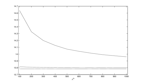
We immediately observe that the predominant part of the upper bias in stems from the subsampling in the approximate construction of the Doob martingales. Without the use of inner control variates, the relative error between upper and lower estimator is about 6% for inner samples and decreases to about 1.5% for inner samples. Application of the inner control variates reduces this relative error to less than 0.25% even in the case of only inner samples.
Table 1 illustrates the influence of different input approximations. It shows realizations of the lower estimator and the upper estimator for the option price as well as the empirical standard deviations, as the number of time steps increases from to . The column on the left explains which algorithm is run for the input approximation. Here, LGW stands for the Lemor-Gobet-Warin algorithm and MB for the martingale basis algorithm. It also states the number of regression samples and the number of basis functions , which are applied in the least-squares Monte Carlo algorithms. The lower and upper price estimates for the Bermudan option case are presented in the last two lines. In this case, the martingale basis algorithm is not available, and the Lemor-Gobet-Warin algorithm is run with the six basis functions stated above. We apply and samples in all cases.
| Algorithm \ | 40 | 80 | 120 | 160 |
By and large, the table shows that in this 5-dimensional example extremely tight 95% confidence intervals can be computed by the primal-dual algorithm, although the input approximations are based on very few, but well chosen, basis functions. For the martingale basis algorithm as input approximation with just two basis functions and 100 regression paths the relative error between lower and upper 95%-confidence bound is about 0.7% even for steps in the time discretization. It can be further decreased to less than 0.5%, when seven basis functions and 1,000 regression paths are applied. If one takes the input approximation of the Lemor-Gobet-Warin algorithm with the same set of basis functions, then the primal-dual algorithm can in principle produce confidence intervals of about the same length as in the case of the martingale basis algorithm. However, in our simulation study the number of regression paths must be increased by a factor of 1,000 in order to obtain input approximations which have the same quality as those computed by the martingale basis algorithm. Hence our numerical results demonstrate the huge variance reduction effect of the martingale basis algorithm. In the Bermudan option case, the primal-dual algorithm still yields 95%-confidence intervals with a relative width of less than 1% for up to time steps, when the input approximation is computed by the Lemor-Gobet-Warin algorithm with 6 basis functions and 1 million regression paths.
5 The case of a non-convex generator
In this section we drop the assumption on the convexity of the generator and merely assume that the standing assumptions are in force. In this situation the construction of confidence bounds for can be based on local approximations of by convex and concave generators.
5.1 Upper bounds
We first turn to the construction of upper bounds. For fixed we assume that some approximation of is given. This approximation can be pre-computed by any algorithm. We merely assume that the approximation is adapted and satisfies
The set of such admissible input approximations is denoted by .
We now choose a measurable function
with the following properties:
-
a)
is adapted for every . Moreover satisfies the stochastic Lipschitz condition
for every (with the same stochastic Lipschitz constants as ).
-
b)
is convex in , for every , and
for every .
Remark 5.1.
Given and the approximation we can define a new generator
Then is convex in and dominates the original generator , i.e. . Moreover,
which shows that – evaluated at the true solution – the auxiliary generator approximates the true generator , as the approximation approaches the true solution.
A generic choice is the function
which obviously satisfies the properties a) and b) above. We will illustrate in the numerical examples below, that it might be beneficial to tailor the function to the specific problem instead of applying the generic choice .
Given , we define via
| (19) | |||||
initiated at . We then obtain the following minimization problem with value process in terms of .
Theorem 5.2.
For every ,
Moreover, a minimizing pair is given by which even satisfies the principle of pathwise optimality.
Proof.
We fix a pair of adapted and integrable processes and define , , as
which satisfies by the comparison result in Proposition 2.3. Then, an application of Theorem 3.1, with replaced by yields . Hence,
It now suffices to show that
-almost surely for every . This is certainly true for . Going backwards in time we obtain by induction
As , we observe that also solves the above equation. Hence, by uniqueness (due to the Lipschitz assumption on ), we obtain . ∎
5.2 Lower bounds
A maximization problem with value process can be constructed analogously by bounding from below by a concave generator. The main difference is that in place of the results of Section 3 we now rely on the following result for the concave case which is proved at the end of this section:
Theorem 5.3.
Suppose is concave in .
(i) Then, for every ,
Minimizers (even in the sense of pathwise optimality) are given by satisfying
| (20) |
and being the martingale part of the Doob decomposition of .
(ii) Given a stopping time and a martingale , define
for
via
Then,
A maximizer (even in the sense of pathwise optimality) is given by the triplet , where was defined in (4) and are the Doob martingales
of and , respectively.
This result is not completely symmetric to the convex case, because the reflection at a lower barrier (i.e. application of the maximum-operator) is convex. Note that if is concave itself then the upper and lower bounds from Theorem 5.3 are preferable to the upper bound of Theorem 5.2 and to the generic lower bounds which are constructed next.
We denote by any mapping which satisfies the same properties as but with condition b) replaced by
-
b’)
is concave in , for every , and
for every .
The generic choice is now
Given , a pair of adapted processes and a stopping time we define via
| (21) | |||||
for initiated at . Making use of Theorem 5.3 and the same arguments as in Theorem 5.2 we obtain:
Theorem 5.4.
For every ,
Moreover, a minimizing triplet is given by which even satisfies the principle of pathwise optimality. (We recall that was defined in (4)).
Example 5.5.
For the generic choices and , we can apply Proposition 3.2 in order to make the recursion formulas in (19) and (21) explicit. They read
and
The main advantage of the corresponding upper and lower bounds is that they can be calculated generically without any extra information on (such as the convex conjugates which were required in the section on convex generators). There is, however, a price to pay for this generic approach. Indeed, given the Lipschitz process , the choice , can be shown to lead to the crudest upper and lower bounds among all admissible functions , , i.e.
for every pair , and analogously for the lower bounds. In practice, the generic bounds may be too crude, when is large and the approximation of is not yet very good. In general we therefore recommend to choose the functions and in a way that and are close to zero in a neighborhood of zero in the -coordinates, in which one expects the residuals to be typically located.
We close this section with the proof of Theorem 5.3.
Proof of Theorem 5.3.
(i) Given and , , define
Then, the optional sampling theorem yields for every stopping time and every martingale
The same argument as in the first part of the proof of Theorem 3.5 now shows by concavity that Hence,
Now we denote the Doob martingale of by for , and choose a pair which satisfies (20). Such a pair exists again by Lemma 3.4. Define
We show by induction on , that . Note first that . In order to prove the claim for we first observe that
for . Hence,
By the induction hypothesis and (20) we obtain
As is the unique solution of this equation we conclude that .
(ii) Fix and . Then, by concavity of we observe analogously to the proof of Theorem 3.1 that
, , is a subsolution to the nonreflected BSDE with generator and terminal time .
The solution of the latter BSDE was denoted by in Proposition 2.2.
Hence, by Propositions 2.3 and 2.2
In order to prove pathwise optimality of one proceeds as in the proof of Theorem 3.1. The analogous induction argument shows that for
which again, by the Lipschitz continuity of , implies . ∎
5.3 Numerical examples
Once the functions and are chosen, an algorithm for computing confidence intervals for based on Theorems 5.2 and 5.4 can be designed analogously to the primal-dual algorithm in Section 4.1 for the convex case.
We first illustrate the algorithm in the context of Example 2.1 (ii). For the underlying, we choose the same five-dimensional geometric Brownian motion as in Section 4.2 except that and the drift and risk-free rate equal . The payoff of the (European) claim is given by . For the default risk function , we assume that there are three regimes, high risk, intermediate risk and low risk: There are thresholds and rates such that for and for . Over , interpolates linearly. The resulting function is Lipschitz continuous but generally neither convex nor concave. The candidates for the Lipschitz constant are the absolute values of the left and right derivatives of in and . In the implementation, we stick to the generic choice
using that the nonlinearity is independent of the -part in this example. We choose
For the calculation of , we use the Lemor-Gobet-Warin algorithm with two basis functions, and , and . Moreover, .
In the absence of default risk, the claim’s value is given by . Table 2 displays upper and lower price bounds for different time discretizations and recovery rates . As expected, a smaller recovery rate leads to a smaller option value. The relative width of the confidence intervals is well below in all cases. For the larger values of , the bounds are even tighter: Larger values of lead to less nonlinearity in the pricing problem and to smaller Lipschitz constants ( for ). Compared to the example of Section 4.2, the bounds are much less dependent on the time discretization. This is due to the fact, that no -part has to be approximated, as is the case for many BSDEs in the credit risk literature, see Crépey et al. (2013); Henry-Labordère (2012). To sum up, the generic approach is perfectly sufficient in this example.
| \ | 40 | 80 | 120 | 160 |
|---|---|---|---|---|
We finally revisit the example of Section 4.2. For the input approximation we run the martingale basis algorithm with seven basis functions for and 1,000 regression paths as specified there. The confidence bounds for the European call spread option on the maximum of five Black-Scholes stocks are calculated with paths based on the following choices of and . For the fully generic implementation we apply
For the semi-generic implementation we choose
This choice only partially exploits the structure of the generator. It can be applied to any generator which is a linear function of plus a nondecreasing -Lipschitz continuous function of a linear combination of . The specific form of the Lipschitz function is not used in this construction of and , but, of course, the coefficients for the linear combinations must be adjusted to the generator in the obvious way. For this semi-generic case the pathwise recursion formulas for and can be made explicit in time analogously to the generic case, which was discussed in Example 5.5.
| Algorithm \ | 40 | 80 | 120 | 160 |
|---|---|---|---|---|
| fully generic | ||||
| semi-generic |
Table 3 shows the resulting low-biased and high-biased estimates for the option price as well as their empirical standard deviations. We observe that the generic bounds are not satisfactory in this example. The relative width of the 95% confidence intervals ranges from about 6.5% for to more than 65% for time steps. This can be explained by the fact that the approximation of by (which is expressed in terms of just two basis functions) is not yet good enough. The quality of plays an all important role for the generic bounds due to the appearance of the terms in the definitions of and . In the semi-generic setting the expressions of the form in and are much more favorable concerning the approximation error of by . Therefore, the semi-generic implementation yields much better 95% confidence intervals with a relative width of about 1% for and still less than 2.5% for time steps.
By and large, this example shows that the generic bounds may be too crude, if applied to good but not excellent approximations , in particular when the -variable of the generator is high-dimensional. Nonetheless very acceptable confidence intervals can still be obtained based on the same approximation , if some information about the generator is incorporated into the choice of and .
Appendix A Continuous time analogues
In this appendix we consider BSDEs driven by a Brownian motion of the form
| (22) |
We assume that the pair are standard parameters in the sense of El Karoui et al. (1997), p. 18, i.e. square-integrability conditions and a uniform Lipschitz condition on are in force. Moreover, is supposed to be convex in .
Then, by Proposition 3.4 in El Karoui et al. (1997)
where is the augmented filtration generated by the driving Brownian motion,
and the supremum runs over the set
This is the non-reflected continuous time analogue to the primal optimization problem in Theorem 3.5 in a Brownian environment.
We now derive a continuous time version of the pathwise approach to the dual minimization problem in Theorem 3.1. On the one hand this continuous time version sheds additional light on the need to use a -dimensional martingale in the upper bound construction in discrete time. On the other hand it might serve as a starting point for the design of alternative upper bound algorithms.
We shall make use of some basic tools from Malliavin calculus. For the corresponding definitions and notations we refer to Nualart (2006). In order to simplify the notation, we assume that the driving Brownian motion is one-dimensional. Given a stochastic process such that is Malliavin differentiable for a.e. , we denote by the Malliavin derivative of . Notice that the field is only defined almost everywhere on , and consequently the trace of is not well-defined. We shall therefore make use of the one-sided trace , as introduced on p. 173 in Nualart (2006) for .
Now given a martingale such that , (i.e. the random variable is Malliavin differentiable with square-integrable Malliavin derivative), we say that a possibly non-adapted process is a -solution of
| (23) |
if , exists, , and for every
Now suppose that is a -solution for some martingale such that . Define , , and
Then,
| (24) |
Assuming that , we next note that
| (25) |
Indeed, by the martingale representation theorem and Lemma 1.3.4 in Nualart (2006), there is an adapted process such that
Then, by Proposition 1.3.8 and the same argument as in Proposition 3.1.1 in Nualart (2006),
The last integral is a martingale increment by adaptedness and square-integrability of the integrand. Hence, taking conditional expectation yields (25). We are now in the position to link to the martingale , which was defined in (24). By the Clark-Ocone formula (Nualart, 2006, Proposition 1.3.14), we obtain
where we used Proposition 1.2.8 from Nualart (2006) to interchange Malliavin derivative and conditional expectation, and (25). Since , we conclude, thanks to (24), that solves the BSDE
By the convexity of we observe that . Hence, by the comparison theorem (see El Karoui et al., 1997, Theorem 2.2), we end up with
Finally, Proposition 5.3 in El Karoui et al. (1997) shows that the unique adapted solution to BSDE (22) satisfies under some technical conditions on and , which we assume from now on. In particular, is a -solution to (23) for . Summarizing the above, we arrive at the following result:
Proposition A.1.
Comparing this result with the discrete time result in Theorem 3.1, we immediately observe a major difference: In continuous time only the choice of a one-dimensional martingale is required, while in discrete time one additionally needs to choose a -dimensional martingale . This phenomenon is easily explained. Notice first that, under at most technical conditions,
where the diamond denotes the Wick product, see Theorem 6.8 in Di Nunno et al. (2009). The first term on the right hand side corresponds to the expression in (5), when equals the truncated Brownian increment over . The second term on the right hand side has zero conditional expectation, because the Wick product interchanges with the conditional expectation, i.e.
see e.g. Lemma 6.20 in Di Nunno et al. (2009). As one cannot expect that the Wick product can be computed in closed form, a generic term with zero conditional expectation, namely the martingale increment , is subtracted in (5). Due to the convexity of , subtracting this generic term with zero conditional expectation pushes the solution of the recursion (5) upwards.
References
- Alanko and Avellaneda (2013) S. Alanko, M. Avellaneda. Reducing variance in the numerical solution of BSDEs. C. R. Math. Acad. Sci. Paris 351, 135–138, 2013.
- Andersen and Broadie (2004) L. Andersen, M. Broadie. A primal-dual simulation algorithm for pricing multidimensional American options. Management Sci. 50, 1222–1234, 2004.
- Bally and Pagès (2003) V. Bally, G. Pagès. A quantization algorithm for solving multi-dimensional discrete-time optimal stopping problems. Bernoulli 9, 1003–1049, 2003.
- Belomestny (2011) D. Belomestny. Pricing Bermudan options by nonparametric regression: optimal rates of convergence for lower estimates. Finance Stoch. 15, 655–683, 2011.
- Belomestny et al. (2009) D. Belomestny, C. Bender, J. Schoenmakers. True upper bounds for Bermudan products via non-nested Monte Carlo. Math. Finance 19, 53–71, 2009.
- Bender and Denk (2007) C. Bender, R. Denk. A forward scheme for backward SDEs. Stochastic Process. Appl. 117, 1793–1812, 2007.
- Bender and Steiner (2012) C. Bender, J. Steiner. Least-squares Monte Carlo for BSDEs. In: Carmona, R. A. et al. (eds.) Numerical Methods in Finance, 257–289, Springer, 2012.
- Bender and Steiner (2013) C. Bender, J. Steiner. A-posteriori estimates for backward SDEs. SIAM/ASA J. Uncertainty Quantification 1, 139–163, 2013.
- Bergman (1995) Y. Z. Bergman. Option pricing with differential interest rates. Rev. Financ. Stud. 8, 475–500, 1995.
- Bouchard and Chassagneux (2008) B. Bouchard, J.-F. Chassagneux. Discrete-time approximation for continuously and discretely reflected BSDEs. Stochastic Process. Appl. 118, 2269–2293, 2008.
- Bouchard and Elie (2008) B. Bouchard, R. Elie. Discrete-time approximation of decoupled forward-backward SDE with jumps. Stochastic Process. Appl. 118, 53–75, 2008.
- Bouchard and Touzi (2004) B. Bouchard, N. Touzi. Discrete-time approximation and Monte Carlo simulation of backward stochastic differential equations. Stochastic Process. Appl. 111, 175–206, 2004.
- Brown et al. (2010) D. B. Brown, J. E. Smith, P. Sun. Information relaxations and duality in stochastic dynamic programs. Oper. Res. 58, 785–801, 2010.
- Chassagneux and Richou (2013) J.-F. Chassagneux, A. Richou. Numerical simulation of quadratic BSDEs. arXiv preprint 1307.5741, 2013.
- Cheridito et al. (2012) P. Cheridito, M. Kupper, N. Vogelpoth. Conditional analysis on . arXiv preprint 1211.0747, 2012.
- Cheridito and Stadje (2013) P. Cheridito, M. Stadje. BSEs and BSDEs with non-Lipschitz drivers: comparison, convergence and robustness. Bernoulli 19, 1047–1085, 2013.
- Cohen and Elliott (2010) S. N. Cohen, R. J. Elliott. A general theory of finite state backward stochastic difference equations. Stochastic Process. Appl. 120, 442–466, 2010.
- Crépey et al. (2013) S. Crépey, R. Gerboud, Z. Grbac, N. Ngor. Counterparty risk and funding: the four wings of the TVA. Int. J. Theor. Appl. Finance 16, 1350006, 2013.
- Crisan and Manolarakis (2012) D. Crisan, K. Manolarakis. Solving backward stochastic differential equations using the cubature method: Application to nonlinear pricing. SIAM J. Financial Math. 3, 534–571, 2012.
- Desai et al. (2012) V. V. Desai, V. F. Farias, C. C. Moallemi. Pathwise optimization for optimal stopping problems. Management Sci. 58, 2292–2308, 2012.
- Duffie et al. (1996) D. Duffie, M. Schroder, C. Skiadas. Recursive valuation of defaultable securities and the timing of resolution of uncertainty. Ann. Appl. Probab. 6, 1075–1090, 1996.
- El Karoui et al. (1997) N. El Karoui, S. Peng, M. C. Quenez. Backward stochastic differential equations in finance. Math. Finance 7, 1–71, 1997.
- Fahim et al. (2011) A. Fahim, N. Touzi, X. Warin. A probabilistic numerical method for fully nonlinear parabolic PDEs. Ann. Appl. Probab. 21, 1322–1364, 2011.
- Gobet and Labart (2007) E. Gobet, C. Labart. Error expansion for the discretization of backward stochastic differential equations. Stochastic Process. Appl. 117, 803–829, 2007.
- Gobet and Makhlouf (2010) E. Gobet, A. Makhlouf. -time regularity of BSDEs with irregular terminal functions. Stochastic Process. Appl. 120, 1105–1132, 2010.
- Guyon and Henry-Labordére (2011) J. Guyon, P. Henry-Labordère. Uncertain volatility model: a Monte Carlo approach. J. Comput. Finance. Published online 22 Feb 2011.
- Haugh and Kogan (2004) M. Haugh, L. Kogan. Pricing American options: a duality approach. Oper. Res. 52, 258–270, 2004.
- Henry-Labordère (2012) P. Henry-Labordère. Cutting CVA’s complexity. Risk Magazine, 67–73, July 2012.
- Johnson (1987) H. Johnson. Options on the maximum or the minimum of several assets. J. Financial Quant. Anal. 22, 277–283, 1987.
- Laurent et al. (2012) J.-P. Laurent, P. Amzelek, J. Bonnaud. An overview of the valuation of collateralized derivative contracts. Rev. Derivatives Res., Online First, 2014.
- Lemor et al. (2006) J.-P. Lemor, E. Gobet, X. Warin. Rate of convergence of an empirical regression method for solving generalized backward stochastic differential equations. Bernoulli 12, 889–916, 2006.
- Ma and Zhang (2005) J. Ma, J. Zhang. Representations and regularities for solutions to BSDEs with reflections. Stochastic Process. Appl. 115, 539 – 569, 2005.
- Nualart (2006) D. Nualart. The Malliavin Calculus and Related Topics, 2nd ed., Springer, 2006.
- Di Nunno et al. (2009) G. Di Nunno, B. Øksendal, F. Proske. Malliavin Calculus for Lévy Processes with Applications in Finance, Springer, 2009.
- Pallavicini et al. (2012) A. Pallavicini, D. Perini, D. Brigo. Funding, collateral and hedging: uncovering the mechanics and the subtleties of funding valuation adjustments. arXiv preprint 1210.3811, 2012.
- Rockafellar (1970) R. T. Rockafellar. Convex Analysis, Princeton University Press, 1970.
- Rogers (2002) L.C.G. Rogers. Monte Carlo valuation of American options. Math. Finance 12, 271–286, 2002.
- Schoenmakers et al. (2013) J. Schoenmakers, J. Zhang, J. Huang. Optimal dual martingales, their analysis, and application to new algorithms for Bermudan products. SIAM J. Financial Math. 4, 86–116, 2013.
- Zhang (2004) J. Zhang. A numerical scheme for BSDEs. Ann. Appl. Probab. 14, 459–488, 2004.
- Zhang et al. (2013) G. Zhang, M. Gunzburger, W. Zhao. A sparse-grid method for multi-dimensional backward stochastic differential equations. J. Comput. Math. 31, 221–248, 2013.