Parameters of the brightest star formation regions in the two principal spiral arms of NGC 628

Abstract

We study photometric properties, chemical abundances and sizes of star formation regions in the two principal arms of the galaxy NGC 628 (M74). The GALEX ultraviolet, optical $UBVRI$, and H$\alpha$ surface photometry data are used, including those obtained with the 1.5-m telescope of the Maidanak Observatory. The thirty brightest star formation regions in ultraviolet light located in the spiral arms of NGC 628 are identified and studied. We find that the star formation regions in one (longer) arm are systematically brighter and larger than the regions in the other (shorter) arm. However, both luminosity and size distribution functions have approximately the same slopes for the samples of star formation regions in both arms. The star formation regions in the longer arm have a higher star formation rate density than the regions in the shorter arm. The regions in the shorter arm show higher N/O ratio at a higher oxygen abundance, but they have lower ultraviolet and H$\alpha$ luminosities. These findings can be explained if we assume that star formation regions in the shorter arm had higher star formation rate in the past, but now it is lower than for those in the opposite arm. Results of stellar evolutionary synthesis show that the brightest regions in the longer arm are slightly younger than the ones in the shorter arm ($3.5\pm 2.2$ Myr versus $6.0\pm 1.1$ Myr). Our results demonstrate that there is a difference in the inner structures and parameters of the interstellar medium between the spiral arms of NGC 628, one of which is long and hosts a regular chain of bright star formation complexes and the other, shorter one does not.

1 Introduction

Star formation regions (H ii regions) are associated with spiral arms of disc galaxies. Within spiral arms of grand design galaxies, star formation regions are often grouped into structures with sizes of about 0.5 kpc, the star complexes (Elmegreen & Lada, 1977; Efremov, 1978, 1979; Elmegreen & Efremov, 1996; Efremov & Elmegreen, 1998). These complexes are the greatest coherent groupings of young stars. Such complexes are formed from H i/H₂ superclouds (Elmegreen & Elmegreen, 1983; Efremov, 1989, 1995; Elmegreen, 1994, 2009; Odekon, 2008; de la Fuente Marcos & de la Fuente Marcos, 2009). The size/mass of the largest star formation regions that can appear in a galaxy is determined by the parameters of the interstellar medium, such as the gas density and pressure (Elmegreen & Efremov, 1997; Kennicutt, 1998a; Billett, Hunter & Elmegreen, 2002; Larsen, 2002).

Occasionally, these star formation complexes are located along an arm at rather regular distances. Elmegreen & Elmegreen (1983) found the spacing of complexes (H ii regions) in studied galaxies to be within 1-4 kpc, and each string to consist, on average, of five H ii regions. Elmegreen & Elmegreen (1983) and Elmegreen (1994) suggested that the gravitational or magneto-gravitational instability developing along the arm can explain this regularity. Elmegreen & Elmegreen (1983) found that in two thirds of cases the regular strings of complexes are seen in one arm only. The well-known galaxy NGC 628 (M74) is the nearest object from the list of Elmegreen & Elmegreen (1983) where the regular spacing of complexes are observed in one arm only. We believe that the study of the properties of such galaxies can help to better understand the nature of the regular chains of bright star formation complexes.

In a previous paper (Gusev & Efremov, 2013, hereafter Paper I) we have studied photometric properties of spiral arms in NGC 628 and location of star formation regions inside these arms. Our results confirmed the conclusion of Elmegreen & Elmegreen (1983), that only one of the spiral arms in NGC 628 has the regular chain of bright star complexes. We also found that the characteristic separation between adjacent fainter star formation regions in both spiral arms of the galaxy is nearly 400 pc (Paper I). The main goal of this new research is to study differences between samples of bright star formation regions in two opposite spiral arms of NGC 628, and to understand why these samples differ from each other. Here, we consider photometric properties, chemical abundances and sizes of the brightest star formation regions in the two principal spiral arms of the grand-design galaxy NGC 628, based on our own observations in the $U$, $B$, $V$, $R$, $I$ passbands, and H$\alpha$ line, as well as the Galaxy Evolution Explorer (GALEX) far- and near-ultraviolet (FUV and NUV) data.

NGC 628 is a nearby spiral galaxy viewed almost face-on (Fig. 1, Table 1). It is an excellent example of a galaxy with regular strings of complexes which are seen in only one arm. Elmegreen & Elmegreen (1983) found seven complexes (H ii regions) with a characteristic separation of 1.6-1.7 kpc in one arm of the galaxy (Fig. 1, Table 2).

Table 1: Basic parameters of NGC 628.

Parameter	Value
Type	SA(s)c
Total apparent $B$ magnitude ($B_{t}$)	$9.70\pm 0.26$ mag
Absolute $B$ magnitude ($M_{B}$)a	-20.72 mag
Inclination ($i$)	$7\degr\pm 1\degr$
Position angle (PA)	$25\degr$
Heliocentric radial velocity ($v$)	$659\pm 1$ km s-1
Apparent corrected radius ($R_{25}$)b	$5.23\pm 0.24$ arcmin
Apparent corrected radius ($R_{25}$)b	$10.96\pm 0.51$ kpc
Distance ($d$)	7.2 Mpc
Galactic absorption ($A(B)_{\rm Gal}$)	0.254 mag
Distance modulus ($m-M$)	29.29 mag

^a Absolute magnitude of the galaxy corrected for Galactic extinction and inclination effect.

^b Isophotal radius (25 mag arcsec^-2 in the $B$-band) corrected for Galactic extinction and absorption due to the inclination of NGC 628.

NGC 628 is a galaxy that has experienced recent star formation episodes. Hodge (1976) identified 730 H ii regions in the galaxy. Sonbaş et al. (2010) found nine supernova remnants (SNRs) in NGC 628 (see Fig. 1). Three supernovae (SN 2002ap, 2003gd, and 2013ej) have been observed in the galaxy since 2001.

NGC 628 is the largest member of a small group of galaxies. The group is centred around NGC 628 and the peculiar spiral NGC 660. NGC 628 is associated with several companions: UGC 1104, UGC 1171, UGC 1176 (DDO13), UGC A20, KDG10, and dw0137+1541. Most of the companions are star-forming dwarf irregulars (Auld et al., 2006). Two giant high velocity gas complexes ($M{\rm(HI)}\sim(0.5-1)\times 10^{8}M_{\odot}$) are located at $\sim 10$ arcmin to the east and to the west from the galactic centre (Kamphuis & Briggs, 1992).

The distance to NGC 628 is still an open question. Sharina, Karachentsev & Tikhonov (1996) obtained 7.2 Mpc based on their observations of the brightest supergiants in NGC 628. The same value was found by van Dyk, Li & Filippenko (2006), who studied the optical curve of SN 2003gd. This value of the distance is in good agreement with the results of McCall, Rybski & Shields (1985) and Ivanov et al. (1992), who studied global properties of NGC 628 and star complexes in it, respectively. An independent determination, based on observations of planetary nebulae, gave a value of 8.6 Mpc (Herrmann et al., 2008). Alternative values, 9.3–9.9 Mpc, were obtained based on studies of SN 2003gd (Hendry et al., 2005; Olivares et al., 2010) and the study of the gravitational stability of the gaseous disc of NGC 628 (Zasov & Bizyaev, 1996). A value close to 10 Mpc is favoured in studies of the NGC 628 Group by Auld et al. (2006). Following the recent studies of e.g. Moustakas et al. (2010), Sonbaş et al. (2010), Aniano et al. (2012) or Berg et al. (2013) we use the value of the distance to NGC 628, obtained in Sharina et al. (1996) and van Dyk et al. (2006). The adoption of an alternative value of the distance, 10 Mpc, will increase the luminosities and the linear distances (sizes) of the objects in NGC 628 by $\sim 30\%$. However, this does not affect the main conclusions of our study, as we compare parameters of star formation regions in the spiral arms of the same galaxy.

The fundamental parameters of NGC 628 are presented in Table 1. We use the position angle and the inclination of the galactic disc derived by Sakhibov & Smirnov (2004). The morphological type and the Galactic absorption, $A(B)_{\rm Gal}$, are taken from the NED data base. Other parameters are taken from the LEDA data base (Paturel et al., 2003). We adopt the Hubble constant $H_{0}=75$ km s^-1Mpc^-1. With the assumed distance to NGC 628, we estimate a linear scale of 34.9 pc arcsec^-1.

The spiral arm with a regular string of complexes found by Elmegreen & Elmegreen (1983) was named Arm A, and the opposite arm was named Arm B (Fig. 1). Arm A is known as Arm 2 in Kennicutt & Hodge (1976) and Cornett et al. (1994) or South arm in Rosales-Ortega et al. (2011).

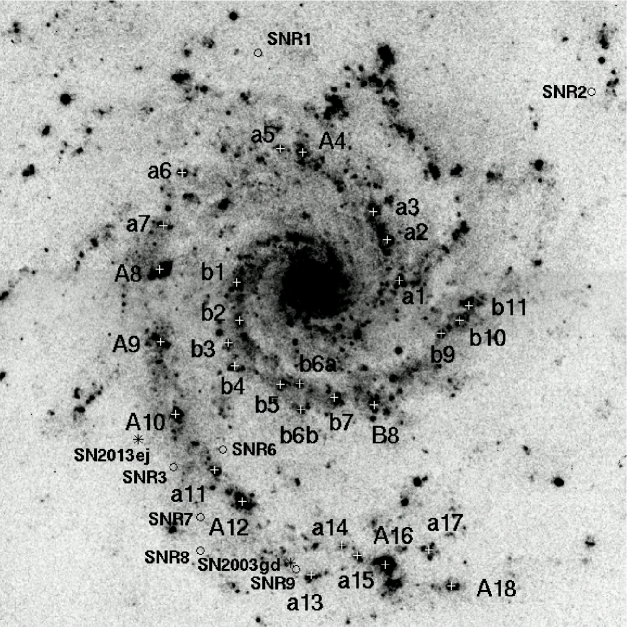
Figure 1: $U$ image of NGC 628 and positions of the galaxy’s star formation regions, supernova remnants, and supernovae. The white crosses show positions of the studied regions. The ID numbers of the star formation regions from Table 2 are indicated. The black circles show positions of the SNRs by Sonbaş et al. (2010), the stars indicate the supernovae. Two supernova remnants (SNR 4 and SNR 5) and SN 2002ap are outside the image field. North is upward and east is to the left. The size of the image is $6.0\times 6.0$ arcmin².

2 Observations and reduction

The results of $UBVRI$ photometry of NGC 628 have already been published in Bruevich et al. (2007). H$\alpha$ spectrophotometric and GALEX ultraviolet photometric observations and data reduction for the galaxy have been described in Paper I. Just a brief compilation is given for these observations and data reduction.

The photometric and spectrophotometric CCD observations were obtained in 2002 ($UBVRI$) and 2006 (H$\alpha$) with the 1.5-m telescope of the Maidanak Observatory (Institute of Astronomy of the Academy of Sciences of Uzbekistan). The focal length of the telescope is 12 m. A detailed description of the telescope and the CCD camera can be found in Artamonov et al. (2010). The images have a pixel scale of 0.267 arcsec pixel^-1. The seeing during the observations was 0.7–1.1 arcsec.

Ultraviolet GALEX FUV and NUV reduced FITS-images of NGC 628 were downloaded from Barbara A. Miculski archive for space telescopes (galex.stsci.edu; source GI3_050001_NGC628). The observations were made in 2007. The description of the GALEX mission and basic parameters of passbands are presented in Morrissey et al. (2005). The image resolution is equal to 4.5 arcsec for FUV and 6.0 arcsec for NUV.

The reduction of the photometric and spectrophotometric data was carried out using standard techniques, with the European Southern Observatory Munich Image Data Analysis System (eso-midas) (Banse et al., 1983; Grøsbol & Ponz, 1990). The main photometric and spectrophotometric image reduction stages were described in detail in Bruevich et al. (2007) and Paper I.

We corrected all data for Galactic absorption using the calibration of Schlafly & Finkbeiner (2011); these values are indicated by the ’0’ subscript. We used the resulting ratio of the extinction in the GALEX bands to the color excess $A_{\rm FUV}/E(B-V)=8.24$ and $A_{\rm NUV}/E(B-V)=8.2$ (Wyder et al., 2007).

To find and select star formation regions, we measured the magnitudes of the brightest regions in the spiral arms of the galaxy. The photometry was made using round apertures, and the light from the surrounding background was subtracted from the light coming from the area occupied by the star formation region. The technique of star formation regions photometry is described in more detail in Gusev & Park (2003) and Bruevich et al. (2007).

Table 2: Offsets and identification of star formation regions in the arms.

Re-	ID	N–Sa	E–Wa	ID1b	ID2c	ID3d	ID4
gion		(arcsec)	(arcsec)
(1)	(2)	(3)	(4)	(5)	(6)	(7)	(8)
1	a1	+2.13	-49.61	—	12	100	—
2	a2	+25.60	-42.68	—	13	—	—
3	a3	+41.60	-34.68	—	14	114	—
4	A4	+75.73	+5.86	—	20	11	1e
5	a5	+77.87	+18.66	—	—	12	—
6	a6	+64.00	+75.19	—	23	29	—
7	a7	+33.60	+85.86	—	—	—	—
8	A8	+8.53	+87.99	A1	60+	30	—
					61
9	A9	-33.07	+87.46	A2	65	53	—
10	A10	-74.67	+78.93	A3	80	61	4e
11	a11	-106.67	+56.53	A4	82	66	—
12	A12	-124.80	+40.53	A5	84	68+	4f
						69
13	a13	-166.94	+1.06	—	91	—	—
14	a14	-149.87	-16.54	—	—	82	—
15	a15	-155.74	-25.61	—	93	84	—
16	A16	-161.07	-41.61	A6	94	83	5f
							6e
17	a17	-152.54	-66.68	—	—	85+	—
						86
18	A18	-173.34	-79.48	A7	—	—	—
19	b1	+1.06	+43.73	—	6	25	6g
20	b2	-20.80	+42.13	—	7	50	—
21	b3	-33.60	+48.53	—	9	52	—
22	b4	-46.94	+44.79	—	67	—	—
23	b5	-57.60	+18.66	—	—	—	—
24	b6a	-57.07	+7.46	—	68	—	—
25	b6b	-72.00	+7.19	—	69	63+	—
						64
26	b7	-65.07	-12.27	—	71	—	—
27	B8	-69.34	-35.21	—	58+	77+	3g
					72	78
28	b9	-28.27	-73.61	—	56	89	2e
							2g
							Ah
29	b10	-20.80	-84.28	—	—	91	—
30	b11	-12.27	-89.61	—	—	92	2g

^a Offsets from the galactic centre, positive to the north and west.

^b ID by Elmegreen & Elmegreen (1983).

^c ID by Rosales-Ortega et al. (2011).

^d ID by Belley & Roy (1992).

^e Ordinal numbers from Table 5 of Berg et al. (2013).

^f ID by Bresolin, Kennicutt & Garnett (1999); the list of Bresolin et al. (1999) coincides with the list of McCall et al. (1985).

^g ID by Gusev et al. (2012).

^h ID by Ferguson, Gallagher & Wyse (1998).

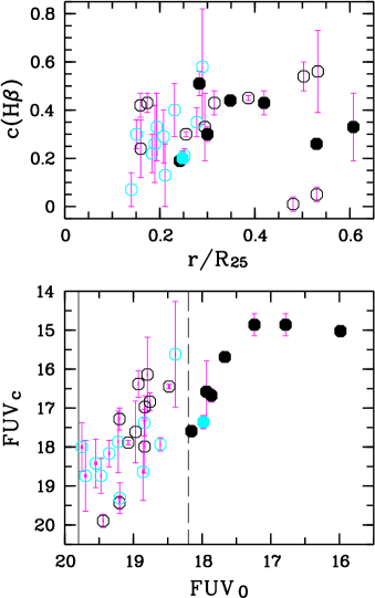
Figure 2: Top panel: radial distribution of interstellar absorption in star formation regions. Bottom panel: comparison between uncorrected and corrected for interstellar absorption magnitudes FUV of the regions. Lower limits of magnitude FUV₀ for bright complexes (dashed line) and star formation regions (solid line) are shown. The black circles denote the regions in Arm A, the grey circles show the objects in Arm B. The filled circles are bright complexes, and the open circles are fainter star formation regions. The magnitudes error bars are shown.

As a result, we selected 30 star formation regions having a total magnitude FUV${}_{0}<19.8$ mag (Fig. 1). The objects were divided into bright complexes and fainter star formation regions. Eight complexes brighter than 18.2 mag in FUV were selected as ’bright complexes’, other 22 objects were named ’star formation regions’. We cut the list of bright complexes on the seventh brightest complex in Arm A; it coincides with the bright H ii regions list of Elmegreen & Elmegreen (1983) but for one exception, our complex A4 is brighter in FUV than the star formation region a11 (Tables 2, 3, Fig. 1). Among regions fainter than 19.8 mag in FUV, we found a large number of diffuse objects without a strong H$\alpha$ emission. Such objects are rather close groups of stellar associations. They have not been investigated in this study. We will show below, that the variation of the limits of brightness does not affect our conclusions in principle.

Spatial location of the star formation regions are shown in Fig. 1. Galactocentric coordinates and identification data of the star formation regions in the arms of NGC 628 are presented in Table 2. Ordinal and identification numbers of the star formation regions are given in columns (1) and (2), respectively. Offsets from the galactic centre are presented in columns (3) and (4), respectively. Identification numbers of the objects by Elmegreen & Elmegreen (1983) are shown in column (5). Most of the selected star formation regions were studied earlier based on spectroscopic and spectrophotometric observations (McCall et al., 1985; Belley & Roy, 1992; Ferguson et al., 1998; Bresolin et al., 1999; Rosales-Ortega et al., 2011; Gusev et al., 2012; Berg et al., 2013). The cross identification data for the complexes are also presented in Table 2. Identification numbers of Rosales-Ortega et al. (2011) are given in column (6), numbers of Belley & Roy (1992) are presented in column (7), and identification numbers of Berg et al. (2013), Bresolin et al. (1999), Ferguson et al. (1998), and Gusev et al. (2012) are given in column (8).

We used a letter-number identification for the star formation regions, the letter ’a’ is used for the regions in Arm A, and the letter ’b’ is used for the objects in Arm B. Bright complexes are marked by a capital letter, and fainter star formation regions are marked by a small one. Sequential numbering is used for the regions in every arm, based on their longitudinal displacements along the arm (Fig. 1, Table 2). Two star formation regions in Arm B are located at the same longitudinal displacement along the spiral arm, they were named ’b6a’ and ’b6b’.

Table 3: Photometric parameters, diameters and galactocentric distances of star formation regions.

ID	$r/R_{25}^{a}$	$r^{b}$	$A^{c}$	FUV0	$M{\rm(FUV)}_{\rm c}$	(FUV-	(NUV-	$(U-B)_{\rm c}$	$(B-V)_{\rm c}$	$(V-R)_{\rm c}$	$(V-I)_{\rm c}$	$\log I$(H$\alpha$)	$c$(H$\beta$)	$d$	$l^{d}$
						${\rm NUV)_{c}}$	$U)_{\rm c}$					([erg  s-1
		(kpc)	(arcsec)	(mag)	(mag)	(mag)	(mag)	(mag)	(mag)	(mag)	(mag)	cm-2])		(pc)	(kpc)
a1	0.159	1.74	12.8	18.84	-12.32$\pm$0.28	0.28$\pm$0.40	0.15$\pm$0.33	-1.01$\pm$0.22	-0.56$\pm$0.19	0.56$\pm$0.16	-0.75$\pm$0.30	-12.94$\pm$0.03	0.42$\pm$0.05e	365$\pm$25	0.85 (a2)
a2	0.160	1.75	9.1	18.84	-11.30$\pm$0.68	0.41$\pm$0.96	0.85$\pm$0.78	-0.69$\pm$0.52	-0.09$\pm$0.43	0.27$\pm$0.34	0.07$\pm$0.31	-12.99$\pm$0.08	0.24$\pm$0.12e	325$\pm$35	0.62 (a3)
a3	0.174	1.90	11.7	18.76	-12.45$\pm$0.23	0.35$\pm$0.32	0.44$\pm$0.26	-0.86$\pm$0.17	-0.22$\pm$0.15	0.19$\pm$0.12	-0.05$\pm$0.12	-12.79$\pm$0.03	0.43$\pm$0.04e	340$\pm$25	0.62 (a2)
A4	0.242	2.65	14.9	18.16	-11.70$\pm$0.11	0.30$\pm$0.16	0.80$\pm$0.13	-0.78$\pm$0.09	-0.07$\pm$0.08	0.39$\pm$0.07	-0.11$\pm$0.09	-12.74$\pm$0.01	0.19$\pm$0.02e	450$\pm$45	0.46 (a5)
a5	0.255	2.80	9.1	19.08	-11.40$\pm$0.06	0.24$\pm$0.08	0.85$\pm$0.07	-0.86$\pm$0.05	-0.22$\pm$0.05	0.45$\pm$0.04	-0.09$\pm$0.05	-12.95$\pm$0.01	0.30$\pm$0.01f	280$\pm$15	0.46 (A4)
a6	0.315	3.45	8.5	19.20	-12.01$\pm$0.28	0.20$\pm$0.40	0.43$\pm$0.33	-1.00$\pm$0.22	-0.31$\pm$0.18	0.27$\pm$0.14	-0.65$\pm$0.14	-13.02$\pm$0.03	0.43$\pm$0.05e	275$\pm$15	1.13 (a7)
a7	0.295	3.23	11.7	18.97	-11.68$\pm$0.79	0.28$\pm$1.12	0.48$\pm$0.91	-0.51$\pm$0.61	-0.30$\pm$0.50	-0.10$\pm$0.39	0.84$\pm$0.35	-13.52$\pm$0.09	0.33$\pm$0.14g	290$\pm$45	0.88 (A8)
A8	0.283	3.10	19.7	17.24	-14.43$\pm$0.28	0.25$\pm$0.40	-0.07$\pm$0.33	-0.75$\pm$0.22	-0.32$\pm$0.18	0.10$\pm$0.14	-0.36$\pm$0.13	-12.46$\pm$0.03	0.51$\pm$0.05e	565$\pm$65	0.88 (a7)
A9	0.300	3.29	16.0	17.86	-12.61$\pm$0.17	0.25$\pm$0.24	0.59$\pm$0.20	-0.56$\pm$0.13	-0.10$\pm$0.11	0.21$\pm$0.08	-0.03$\pm$0.08	-12.78$\pm$0.02	0.30$\pm$0.03e	445$\pm$30	1.45 (A8)
A10	0.348	3.82	13.9	17.67	-13.60$\pm$0.11	0.25$\pm$0.16	0.10$\pm$0.13	-0.94$\pm$0.09	-0.25$\pm$0.07	0.23$\pm$0.06	-0.10$\pm$0.05	-12.56$\pm$0.01	0.44$\pm$0.02e	495$\pm$40	1.36 (a11)
a11	0.386	4.23	13.9	18.48	-12.84$\pm$0.06	0.24$\pm$0.08	0.26$\pm$0.07	-0.80$\pm$0.04	-0.27$\pm$0.04	0.28$\pm$0.03	-0.23$\pm$0.03	-12.72$\pm$0.01	0.45$\pm$0.01e	405$\pm$35	0.84 (A12)
A12	0.419	4.60	20.8	16.78	-14.43$\pm$0.28	0.22$\pm$0.40	0.16$\pm$0.33	-0.85$\pm$0.22	-0.16$\pm$0.18	0.28$\pm$0.14	-0.09$\pm$0.13	-12.16$\pm$0.03	0.43$\pm$0.05e	570$\pm$20	0.84 (a11)
a13	0.532	5.83	10.7	18.80	-13.15$\pm$0.96	0.20$\pm$1.36	-0.08$\pm$1.11	-0.92$\pm$0.74	-0.33$\pm$0.60	0.02$\pm$0.47	0.09$\pm$0.43	-13.11$\pm$0.11	0.56$\pm$0.17e	335$\pm$20	0.86 (a14)
a14	0.481	5.27	7.5	19.44	-9.39$\pm$0.17	0.00$\pm$0.24	1.31$\pm$0.20	-0.70$\pm$0.13	-0.17$\pm$0.11	0.33$\pm$0.09	0.39$\pm$0.08	-13.68$\pm$0.02	0.01$\pm$0.03f	260$\pm$15	0.38 (a15)
a15	0.503	5.51	10.7	18.93	-12.91$\pm$0.34	0.15$\pm$0.48	0.03$\pm$0.39	-0.82$\pm$0.26	-0.29$\pm$0.21	0.39$\pm$0.17	0.19$\pm$0.15	-12.83$\pm$0.04	0.54$\pm$0.06e	280$\pm$40	0.38 (a14)
A16	0.530	5.81	28.3	15.98	-14.27$\pm$0.06	0.18$\pm$0.08	0.49$\pm$0.07	-0.74$\pm$0.04	-0.03$\pm$0.04	0.19$\pm$0.03	0.09$\pm$0.03	-12.03$\pm$0.01	0.26$\pm$0.01e	795$\pm$40	0.59 (a15)
a17	0.530	5.81	14.4	19.20	-9.86$\pm$0.17	0.14$\pm$0.24	1.37$\pm$0.20	-0.66$\pm$0.13	0.05$\pm$0.11	0.30$\pm$0.09	0.42$\pm$0.08	-13.44$\pm$0.02	0.05$\pm$0.03f	350$\pm$20	0.85 (A18)
A18	0.607	6.66	13.9	17.94	-12.71$\pm$0.79	0.12$\pm$1.12	0.28$\pm$0.91	-0.81$\pm$0.61	-0.09$\pm$0.50	0.06$\pm$0.39	-0.10$\pm$0.35	-12.92$\pm$0.09	0.33$\pm$0.14g	410$\pm$30	0.85 (a17)
b1	0.140	1.54	12.8	19.20	-9.98$\pm$0.40	0.32$\pm$0.56	1.33$\pm$0.46	-0.53$\pm$0.31	0.05$\pm$0.26	0.14$\pm$0.22	0.12$\pm$0.22	-13.42$\pm$0.05	0.07$\pm$0.07e	290$\pm$30	0.77 (b2)
b2	0.151	1.65	9.1	19.35	-11.12$\pm$0.34	0.40$\pm$0.48	0.83$\pm$0.39	-0.62$\pm$0.26	0.03$\pm$0.21	0.19$\pm$0.17	-0.04$\pm$0.16	-13.15$\pm$0.04	0.30$\pm$0.06e	250$\pm$15	0.50 (b3)
b3	0.189	2.08	9.1	19.70	-10.55$\pm$0.91	0.31$\pm$1.28	0.98$\pm$1.04	-1.00$\pm$0.69	-0.42$\pm$0.58	0.24$\pm$0.47	-0.47$\pm$0.47	-13.34$\pm$0.11	0.26$\pm$0.16e	235$\pm$20	0.48 (b4)
b4	0.208	2.28	11.7	19.55	-10.87$\pm$0.62	0.29$\pm$0.88	0.86$\pm$0.72	-0.52$\pm$0.48	-0.44$\pm$0.39	-0.07$\pm$0.32	-0.25$\pm$0.30	-14.06$\pm$0.08	0.29$\pm$0.11e	270$\pm$30	0.48 (b3)
b5	0.193	2.12	10.1	19.22	-11.42$\pm$0.79	0.33$\pm$1.12	0.69$\pm$0.91	-0.35$\pm$0.61	-0.12$\pm$0.50	0.11$\pm$0.39	0.00$\pm$0.36	-13.53$\pm$0.09	0.33$\pm$0.14g	245$\pm$35	0.39 (b6a)
b6a	0.184	2.01	8.0	19.47	-10.55$\pm$0.45	0.31$\pm$0.64	0.95$\pm$0.52	-0.54$\pm$0.35	-0.10$\pm$0.29	0.31$\pm$0.24	0.38$\pm$0.22	-13.34$\pm$0.05	0.22$\pm$0.08e	240$\pm$30	0.39 (b5)
b6b	0.231	2.53	11.2	19.75	-11.29$\pm$0.62	0.26$\pm$0.88	0.76$\pm$0.72	-0.87$\pm$0.48	-0.09$\pm$0.39	0.26$\pm$0.31	-0.07$\pm$0.29	-13.14$\pm$0.07	0.40$\pm$0.11e	225$\pm$35	0.52 (b6a)
b7	0.211	2.31	13.3	18.86	-10.65$\pm$0.74	0.28$\pm$1.04	1.26$\pm$0.85	-0.44$\pm$0.56	0.04$\pm$0.46	0.06$\pm$0.36	0.24$\pm$0.33	-13.55$\pm$0.09	0.13$\pm$0.13e	330$\pm$25	0.73 (b6b)
B8	0.248	2.71	18.7	17.98	-11.93$\pm$0.17	0.32$\pm$0.24	0.91$\pm$0.20	-0.70$\pm$0.13	-0.14$\pm$0.11	0.24$\pm$0.10	-0.02$\pm$0.11	-12.72$\pm$0.02	0.20$\pm$0.03e	445$\pm$65	0.82 (b7)
b9	0.252	2.76	12.8	18.61	-11.36$\pm$0.17	0.37$\pm$0.24	1.03$\pm$0.20	-0.60$\pm$0.13	0.22$\pm$0.11	0.45$\pm$0.09	0.14$\pm$0.08	-12.67$\pm$0.02	0.21$\pm$0.03e	305$\pm$30	0.46 (b10)
b10	0.278	3.04	12.3	18.84	-11.92$\pm$0.34	0.33$\pm$0.48	0.62$\pm$0.39	-0.38$\pm$0.26	-0.07$\pm$0.21	0.09$\pm$0.17	-0.09$\pm$0.16	-13.27$\pm$0.04	0.35$\pm$0.06f	325$\pm$45	0.35 (b11)
b11	0.290	3.17	12.8	18.39	-13.67$\pm$1.36	0.28$\pm$1.92	0.05$\pm$1.56	-0.64$\pm$1.04	-0.21$\pm$0.85	0.11$\pm$0.67	0.05$\pm$0.60	-12.85$\pm$0.16	0.58$\pm$0.24h	400$\pm$25	0.35 (b10)

^a Deprojected galactocentric distance normalized to the disc isophotal radius $R_{25}$.

^b Deprojected galactocentric distance.

^c Diameter of the aperture.

^d Distance to the nearest neighbour, the ID numbers of the nearest star formation regions/complexes are shown in the brackets.

^e Rosales-Ortega et al. (2011).

^f Belley & Roy (1992).

^g Mean for the regions from our list by data of Rosales-Ortega et al. (2011).

^h Gusev et al. (2012).

3 Star formation regions in the arms

3.1 Photometric parameters of star formation regions

Results of photometric observations of the star formation regions using a round aperture are given in Table 3. Magnitudes and H$\alpha$ fluxes in this table are corrected for interstellar absorption. Taking into account the interstellar absorption is extremely important for obtaining real luminosities and colour indices and study the physical parameters of star formation regions. We used a logarithmic extinction coefficient, $c$(H$\beta$), obtained from spectroscopic and spectrophotometric observations, to correct the photometric data for interstellar absorption in the regions (see Table 2). The reddening function of Cardelli, Clayton & Mathis (1989) was adopted, assuming $R\equiv A_{V}/E(B-V)=3.1$, for correction of fluxes in optical bands, and data of Wyder et al. (2007) were used for correction of fluxes in ultraviolet bands.

The most complete contemporary study of spectral parameters of H ii regions was carried out by Rosales-Ortega et al. (2011), who used data of integral field spectroscopy of NGC 628. Estimations of logarithmic extinction coefficients for most of objects, studied here, were derived by Rosales-Ortega et al. (2011). These estimations are used in the present paper. For other objects we accept estimations of $c$(H$\beta$) from Belley & Roy (1992) and Gusev et al. (2012). Note that the accuracy of $c$(H$\beta$) estimations derived from spectrophotometric observations of Belley & Roy (1992) is lower than the ones based on the spectroscopy. There are no spectroscopic or spectrophotometric observations for three objects (a7, A18, b5). For these regions, we use $c$(H$\beta$) = $0.33\pm 0.14$ as the mean value for the complexes in our list. Adopted $c$(H$\beta$) are presented in Table 3.

Colour indices and H$\alpha$ fluxes, corrected for interstellar absorption absolute magnitudes, are presented in Table 3. The interstellar absorption, calculated using $c$(H$\beta$), includes the Galactic extinction, the internal extinction due to the interstellar medium within NGC 628, and the intergalactic extinction due to the intergalactic medium between the Milky Way and NGC 628. These values are indicated by ’c’ subscript.

The main contribution to the inaccuracy of magnitudes, corrected for interstellar absorption, is related to the uncertainty in the extinction coefficient, especially in the short wavelength bands. Obviously, the results of photometry can be used only for qualitative comparison of physical parameters of the star formation regions in Arms A and B.

After correction for interstellar absorption, as we can see from Fig. 2, some ’bright’ complexes become fainter than some ’faint’ star formation regions and vice versa. However, it does not affect the following conclusions. Below we study samples of brightest star formation regions in Arms A and B without a division of objects in ’bright complexes’ and ’star formation regions’.

The value of interstellar absorption in star formation regions of Arm A and Arm B is approximately the same: $\langle c$(H$\beta$)$\rangle=0.35\pm 0.15$ versus $0.28\pm 0.13$. It does not depend on the galactocentic distance for regions in Arm A, $\langle c$(H$\beta$)$\rangle=0.35\pm 0.10$ for regions with $r/R_{25}<0.32$ and $0.34\pm 0.20$ for regions with $r/R_{25}>0.32$ (Fig. 2). Note a large variation of $c$(H$\beta$) for objects at the end of Arm A (Fig. 2).

Thus, photometric data, corrected for interstellar absorption, support that young stellar objects (both complexes and star formation regions) in Arm A are systematically brighter than the ones in Arm B of NGC 628. Below we will discuss the physical reasons of such differences.

Star formation regions in Arm A are bluer than the ones in Arm B (Figs. 3, 4). Differences between colour properties of regions in the arms decrease toward long wavelength passbands. Two relatively well defined groups of regions appear in the ultraviolet colour-magnitude diagram, (FUV-NUV)_c vs. $({\rm NUV}-U)_{\rm c}$ and $(U-B)_{\rm c}$ vs. $(B-V)_{\rm c}$ two-colour diagrams, and are mixed in the $(B-V)_{\rm c}$ vs. $(V-R)_{\rm c}$ and $(B-V)_{\rm c}$ vs. $(V-I)_{\rm c}$ two-colour diagrams (Figs. 3, 4).

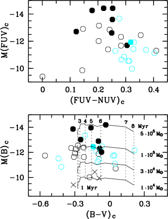
Figure 3: $M({\rm FUV})_{\rm c}$ vs. (FUV-NUV)_c (top) and $M(B)_{\rm c}$ vs. $(B-V)_{\rm c}$ (bottom) colour-magnitude diagrams for regions in arms of NGC 628. Evolutionary tracks of synthetically aged stellar systems of different masses (solid curves) are shown. The dotted lines are isochrones of synthetic stellar systems. The diagonal crosses show open star clusters in the Milky Way by data of Kharchenko et al. (2009). Other symbols are the same as in Fig. 2. See the text for details.

In Fig. 3 (bottom) we compare the observed colour-magnitude relations obtained in $B$ and $V$ passbands for studied objects with the prediction of standard SSP-models (Stellar population synthesis model predictions). A number of SSP-models have been constructed during the last decade. They are widely used for modelling both star clusters and galactic populations. Photometric properties of model clusters are defined by the implemented grid of isochrones. Here we use the grid provided by the Padova group (Bertelli et al., 1994; Girardi et al., 2000; Marigo & Girardi, 2007; Marigo et al., 2008) via the online server CMD. The latest Padova models (version 2.5), described in Bressan et al. (2012), are computed for the narrower interval of initial masses ranges from 0.1 $M_{\odot}$ to 12 $M_{\odot}$. For our purposes we need the interval of initial masses ranges up to 100 $M_{\odot}$. That is the reason, why we used the prior sets of stellar evolutionary tracks (version 2.3), described in Marigo et al. (2008) and computed for the wide interval of initial masses ranges from 0.15 $M_{\odot}$ to 100 $M_{\odot}$.

We used a metallicity grid with $Z=0.012$ which is close to the mean chemical abundance of H ii regions in NGC 628, and retrieved the passbands $B$, $V$ an age range $\log t=6.0-10.2$ and a step of 0.05 in $\log t$. Calculations of integrated $L_{B}$ and $L_{V}$ fluxes are performed for the case of a continuous populated IMF and simultaneous star formation, according to the method described in the paper by Piskunov et al. (2009). We computed a number of models for the different mass values of star clusters from $10^{4}M_{\odot}$ up to $3.5\times 10^{5}M_{\odot}$. We assumed a Salpeter value of the slope $\alpha=-2.35$ and low mass limit $m_{l}=0.1M_{\odot}$ of the IMF. The upper limit $m_{l}=100M_{\odot}$ of the IMF is limited by the used evolutionary grid. Fig. 3 shows four evolutionary tracks computed for different masses of the model and for the age interval from 1 Myr up to 8 Myr. These parameters were chosen to provide a fit of the colour distribution on the colour-magnitude diagram.

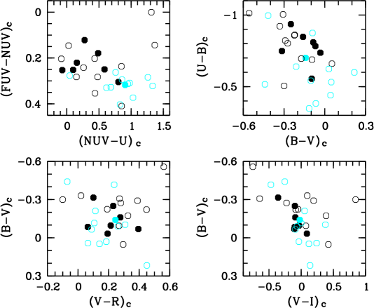
Figure 4: Two-colour diagrams for the star formation regions in the arms of NGC 628. Symbols are the same as in Fig. 2.

About $80\%$ of the luminosity of star formation regions in the $B$ band is provided by high mass stars ($m>4M_{\odot}$). The $B-V$ colour indices of these massive stars are approximately similar within the main sequence at fixed age. One can see that isochrones of synthetic clusters of different masses in the colour-magnitude diagram (Fig. 3, bottom) are perpendicular to the $B-V$ axis. The young massive regions studied here may be made of several star clusters produced in a single episode of star formation and having identical ages and thereby have identical $B-V$ colour indices of the brightest stars. It means that the multiple structure of unresolved star forming regions does not influence the integrated $B-V$ colour indices of unresolved star formation regions. In case of $U-B$ colours, the mass dispersion of individual clusters embedded into the unresolved star formation regions leads to slight reddening of the integrated $U-B$ colour indices and thereby to older ages.

Since we use the $B$ luminosities and integrated $B-V$ colours of unresolved star formation regions in the colour-magnitude diagram, we can assign parameters of the model of the single massive cluster to the unresolved multiple star clusters.

Fig. 3 shows that all studied objects are younger than 8 Myr. The figure shows also that typical mass interval of studied star formation regions are within the range from $1\times 10^{4}M_{\odot}$ up to $\approx 5\times 10^{5}M_{\odot}$. The lower limit of the mass interval overlaps with the upper mass limit of open star clusters (OSCs) in the Milky Way. The three brightest complexes in Arm A (A8, A12 and A16) have approximately the same luminosity. The synthetic evolutionary tracks show that the mass of these complexes is $5\times 10^{5}M_{\odot}$ (Fig. 3). The upper limit of the mass interval is close to masses of young massive star clusters in nearby galaxies (Larsen et al., 2011).

Results of stellar evolutionary synthesis show that star formation regions in Arm A are slightly younger than the ones in Arm B. Excluding the three bluest star formation regions located outside the evolutionary tracks in Fig. 3 (bottom), we found that the mean age of the young stellar objects in Arm A is $3.7\pm 2.2$ Myr versus $6.0\pm 1.1$ Myr for the star formation regions in Arm B. Note that the star formation regions in Arm A are younger than the complexes ($3.0\pm 2.2$ Myr versus $4.7\pm 1.9$ Myr).

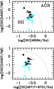
Figure 5: Emission-line diagnostic diagrams for star formation regions in Arm A and Arm B. The curves represent upper boundaries for photoionized nebulae defined by Kewley et al. (2006). Symbols are the same as in Fig. 2.

3.2 Chemical abundances of star formation regions

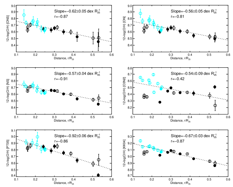
Figure 6: Radial distribution of oxygen abundances in the galaxy. Oxygen abundances were obtained using six empirical methods (see text). Symbols are the same as in Fig. 2.

We selected a homogeneous sample of star formation regions, which have been studied using integral field spectroscopy techniques (Rosales-Ortega et al., 2011). The sample includes 22 regions out of 30 in both arms (see column (6) in Table 2).

The aim of this section is to compare the metallicities of the ionized gas of star formation regions located in different spiral arms. Oxygen is the most abundant heavy element in interstellar medium, so its abundance is the best indicator of gas metallicity.

It is useful to study the nitrogen-to-oxygen abundances ratio in galaxies for understanding their chemical evolution due to the difference of nature of these elements. Nitrogen is ejected into interstellar medium by both low- and intermediate-mass stars and massive stars, whereas oxygen is created only in the last ones. Analysis of O/N–O/H plane may allow us to arrive to conclusions about star formation rate and history of star-forming galaxies (Mollá et al., 2006).

The most accurate way to estimate the oxygen and nitrogen abundance is the so-called ’direct’ temperature-based method. However, the direct method is unavailable for the objects, studied here, because of the absence of temperature-sensitive auroral lines, such as [O iii] $\lambda 4363$. We used several most popular empirical methods: ONS, ON (Pilyugin, Vílchez & Thuan, 2010) and NS (Pilyugin & Mattsson, 2011). Oxygen abundance have been estimated also by PT05 (Pilyugin & Thuan, 2005), O3N2 (Pettini & Pagel, 2004) and KK04 (Kobulnicky & Kewley, 2004) empirical methods.

At this point, the following question arises: do methods calibrated on pure H ii regions or on photoionization models give reliable estimations when applied to real star formation regions in NGC 628? To answer this question, we plotted the traditional [O iii] $\lambda$5007/H$\beta$ versus [N ii] $\lambda$6584/H$\alpha$ and [S ii] $\lambda$6717, 6731/H$\alpha$ diagnostic diagrams for investigated regions in Arms A and B in Fig. 5. Dashed lines denote upper boundaries for photoionized nebulae defined by Kewley et al. (2006). As one can see from this figure, all regions lie within the photoionization area and do not show signatures of shock excitation. This indicates that the empirical methods used are reliable.

Another feature that is clearly seen from Fig. 5 is that complexes from Arm B have lower [O iii]/H$\beta$ values than those from Arm A for the same ratio of [S ii]/H$\alpha$ and [N ii]/H$\alpha$. This can be easily explained by the lower ionisation parameter in regions from Arm B (see, for example, photoionisation models constructed by Levesque, Kewley & Larson, 2010).

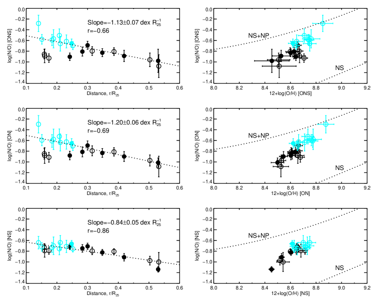
Figure 7: N/O gradient of investigated star formation regions with their distance from the centre (left) and with oxygen abundance O/H (right). Abundances were obtained using three empirical methods (see text). Dashed lines on the right panels show possible boundaries for data points on the N/O–O/H plane under the assumption of close box model for secondary (NS) and both primary and secondary (NS+NP) nitrogen. Symbols are the same as in Fig. 2.

In recent years, several authors performed detailed comparisons of abundance estimation methods and found their discrepancies (see e.g. Kewley & Ellison, 2008, and references therein). López-Sánchez et al. (2012) analysed model spectra of H ii regions and showed that theoretical methods, such as KK04, give overestimated values of oxygen abundance in comparison with ’direct’ $T_{e}$ method, whereas empirical ON, NS and ONS methods are in good agreement. Investigations of individual H ii regions in nearby galaxies confirm that result (see e.g. Egorov, Lozinskaya & Moiseev, 2013). The situation is similar for star formation complexes in NGC 628 (see Fig. 6). Oxygen abundances obtained by KK04 and O3N2 are slightly higher than those obtained by PT05, ON, ONS and NS methods. Possibly, this fact may be due to the large size of investigated regions, where local temperature inhomogeneities play an important role and have to be taken into account.

The oxygen abundance distribution along the radius of the galaxy shows a significant gradient. It was studied by Rosales-Ortega et al. (2011) using 4 methods of abundance determination, including O3N2 and KK04. We estimated oxygen abundance gradient by linear $\chi^{2}$ fitting of data points obtained with six empirical methods. The results are shown in Fig. 6. The absolute value of the correlation coefficient, $r$, for almost all dependences shown in Fig. 6 is greater than 0.8 that corresponds to a fine linear approximation. There is only one exception – the O3N2 abundance versus distance where $r=-0.42$ and abundance measurements show a wide spread. It is not surprising because the accuracy of the O3N2 method is lower than of other applied methods (about 0.2 dex in comparison with 0.1 dex for other). The values of the gradient obtained are in good agreement for the ONS, ON, NS and PT05 methods, slightly higher for KK04 and much higher for O3N2 methods. Note that the slope of O/H dependence on radius obtained by KK04 method is in good agreement with Rosales-Ortega et al. (2011) estimations. This is not surprising because we used their reported fluxes. But our gradient, that we obtained with O3N2 method, is much steeper than the one reported by Rosales-Ortega et al. (2011). This may be caused by using only a small sample of their data points.

Fig. 7 shows the N/O ratios as a function of the distance from the galaxy centre (left-hand panels) and the oxygen abundances (right-hand panels) obtained with the ONS, ON and NS methods. Note that the N/O ratios with the galactocentric radius shown in Fig. 7 are in good agreement with the results of Berg et al. (2013), who found the extrapolated central N/O ratio $-0.45\pm 0.08$ dex and the slope of the N/O ratio gradient $-1.10\pm 0.14$ dex $R_{25}^{-1}$ within the optical radius, $R_{25}$. Analysis of these dependences may be of help in answering the question on the nature of the nitrogen in the star formation complexes under study. If nitrogen is mostly primary (NP), then N/O ratio should be constant, but if it is secondary, the N/O ratio grows with oxygen abundance increase. Fig. 7 shows exactly the same linear dependence. Moreover, the variation of the N/O gradient with the galactocentric radius is steeper than for $12+\log(\mathrm{O/H})$. This can be interpreted as evidence of the predominantly secondary nature of nitrogen in the star formation complexes under study. The trend in the evolution of the ratio N/O with $12+\log(\mathrm{O/H})$ shown in Fig. 7 (right-hand panels) is in good agreement with those found in other Sc-type galaxies (Villa-Costas & Edmunds, 1993).

Fig. 7 shows a clear separation between the properties of the star formation regions hosted by Arm A and Arm B. The regions from Arm B show higher N/O ratio at a higher oxygen abundance. It was shown recently (see e.g. Mollá & Gavilán, 2010; Mallery et al., 2007) that the location of a region in the N/O–O/H plane is related to the specific star formation rate, SFR, per unit mass in stars (sSFR). The higher values of N/O correspond to the smaller sSFR. If the sSFR is small, star formation could have been high in the past, at the earlier times of evolution. The gas was consumed and therefore the SFR decreased and is now small. And conversely, when the efficiency to form stars is low, the star formation rate increases over time and the present SFR is high. So, the N/O–O/H planes in Fig. 7 may be explained if we propose that complexes in Arm B had a higher SFR in the past, but now it is lower than for Arm A. As we will see further, that is possibly our case (see Fig. 11).

There are several regions from Arm A and Arm B that have similar oxygen abundance, but different N/O ratios. All three methods, used to estimate these values, give similar results – complexes from Arm B have slightly higher N/O ratios for a given $12+\log(\mathrm{O/H})$. This may be easily explained if regions from Arm A are younger than those from Arm B. In that case nitrogen could not enrich the interstellar medium in Arm A because of the delay of the nitrogen appearance in the interstellar medium with respect to oxygen. This is supported by the results of Sonbaş et al. (2010). Their search for supernova remnants in NGC 628 gave nine SNR candidates, five of them in Arm A. Two out of three latest supernovae are also located in Arm A (see Fig. 1).

3.3 Star formation region luminosity function

The distribution of star formation regions by mass, as well as an upper limit for the mass of these regions, depends on properties of interstellar medium such as gas density and pressure and correlates with the overall star formation rate (Elmegreen & Efremov, 1997; Kennicutt, 1998a; Billett et al., 2002; Larsen, 2002). Nevertheless, most studies of properties of star formation region populations have focused on the model-independent luminosity function (see e.g. Haas et al., 2008; Mora et al., 2009).

In order to further compare the properties of the star formation regions in Arms A and B, we have constructed the luminosity function for the brightest relevant objects in both arms. In contrast to Larsen (2002), Haas et al. (2008) and Mora et al. (2009), we used ultraviolet luminosities, as they are most sensitive to the presence of young stellar populations. A standard power-law luminosity function of the form

$$dN(L_{\rm FUV})/dL_{\rm FUV}=\beta L_{\rm FUV}^{\alpha}$$ (1)

was adopted. It was converted to the form

$$\log N=a{\rm FUV}+b$$ (2)

for the fitting, where the variables $\alpha$, $\beta$ in Eq. (1) and $a$, $b$ in Eq. (2) are related as $\alpha=-2.5a-1$ and $\beta=2.5(\ln 10)^{-1}10^{b+4.8a}$, respectively.

The constructed star formation region luminosity functions are shown in Fig. 8. Each histogram was fitted using the normal least-squares method to an expression of the form of Eq. (2). The results of the fitting are summarised in Table 4.

Usually, researchers of cluster luminosity functions obtain internal extinction coefficients from evolutionary synthesis models (Larsen, 2002; Mora et al., 2009). The luminosity functions of the star formation regions have been obtained using both corrected and uncorrected (for interstellar absorption) magnitudes. The interstellar absorption coefficients are model-independent. We can only provide a rough estimate of the slope of the luminosity function for the brightest star formation regions in the spiral arms because of the small number statistics.

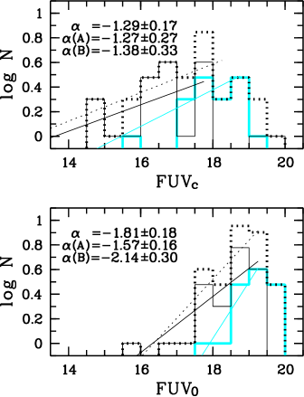
Figure 8: Luminosity functions for the regions using corrected for internal absorption (top panel) and uncorrected FUV magnitudes (bottom panel). Thick dotted histograms are luminosity functions for the regions in both arms, thin black solid histograms are functions for the regions in Arm A, and thick grey histograms are functions for the regions in Arm B. Black dotted, black solid, and grey solid straight lines represent the power-law fit of the form of Eq. (1) for the samples of star formation regions in both arms, Arm A and Arm B, respectively.

Table 4: Luminosity function coefficients.

Arm	$\alpha$	$a$	$b$	Fit interval
A	-1.27$\pm$0.27	0.11$\pm$0.11	-1.46$\pm$1.74	FUV${}_{\rm c}<18.0$
B	-1.38$\pm$0.33	0.15$\pm$0.13	-2.30$\pm$1.50	FUV${}_{\rm c}<19.0$
A+B	-1.29$\pm$0.17	0.12$\pm$0.07	-1.50$\pm$1.14	FUV${}_{\rm c}<18.5$
A	-1.57$\pm$0.16	0.23$\pm$0.06	-3.72$\pm$1.10	FUV${}_{0}<19.5$
B	-2.14$\pm$0.30	0.46$\pm$0.12	-8.18$\pm$2.29	FUV${}_{0}<19.5$
A+B	-1.81$\pm$0.18	0.32$\pm$0.07	-5.17$\pm$1.24	FUV${}_{0}<19.5$

Obtained slopes of luminosity function, based on an uncorrected FUV data, differ for the region population in Arm A and B (Fig. 8). The slope for the region population in Arm B is typical for brightest young cluster populations in galaxies (Zepf et al., 1999; Whitmore et al., 1999; Larsen, 2002; Dolphin & Kennicutt, 2002; de Grijs et al., 2003; Gieles et al., 2006; Haas et al., 2008; Mora et al., 2009). A more gently sloping function is obtained for the star formation region population in Arm A. A value of the slope $\alpha=-1.5$ is close to the results of van den Bergh & Lafontaine (1984) for the Milky Way open clusters, Whitmore et al. (1999) and Haas et al. (2008) for faint clusters in the Antennae and M51, respectively. The united population of star formation regions have an intermediate slope of luminosity function (Fig. 8).

A surprising result was obtained for the star formation region luminosity function when we used corrected FUV magnitudes. The same, within errors, shallow slope is found for the star formation regions population in both spiral arms. The flat distribution can be a result of selection; we lost objects with high extinction, which are slightly fainter than 19.7 mag in FUV. However, this effect must be the same for the star formation regions populations in both arms. Note that the large error in the slope for the star formation regions sample in Arm B is due to the large uncertainty of corrected FUV magnitude of the brightest star formation region b11 (see Table 3).

3.4 Sizes and size distribution functions of star formation regions

To measure sizes of the star formation regions, we used the following technique: (i) the mean intensity level of the background in FUV, $\langle F\rangle$, and its standard deviation, $\sigma$, within the arms but outside the star formation regions were found, (ii) the cutoff intensity, $F_{\rm cut}=\langle F\rangle+5\sigma$ was calculated, (iii) all pixels in the FUV image with the intensity $F>F_{\rm cut}$ were selected. The cutoff intensity $F_{\rm cut}$ corresponds to a surface brightness $\mu({\rm FUV}_{0})=23.68\pm 0.10$ mag arcsec^-2. Areas within Arms A and B with a surface brightness level higher than 23.63 mag arcsec^-2 in FUV were identified and measured (Fig. 9). We found 56 regions in total. Characteristic diameters $d$ of star formation regions were defined as

$$d=2\sqrt{S/\pi},$$

where $S$ is the area of selected regions. Diameters of star formation regions from our sample are given in the last column of Table 3. Errors in determining the diameters of the objects are caused by the accuracy of determining the value of $F_{\rm cut}$.

Arm A is twice as long as Arm B. To compare the size distribution of the regions in Arms A and B on the same galactocentic distance range, we divided Arm A into inner (A1) and outer (A2) parts. The end of inner part of Arm A corresponds to the end of Arm B (Fig. 9). It looks like the inner part of Arm A (A1) and Arm B in Fig. 9 are ’classic’ spiral arms – as regards to their inner structure they are similar and seems to be that both arms show the same age (composition) gradient across the arm. They also have approximately the same length.

The characteristic diameters of 30 star formation regions from our samples are in the range 225–800 pc (Table 3), the diameters of the other 26 star formation regions are smaller, 30 pc $<d<$ 250 pc.

The three brightest star formation complexes in Arm A (A8, A12 and A16) have characteristic diameters $d>500$ pc. All these complexes are double in reality, as seen in $U$ and H$\alpha$ images of the galaxy (Figs. 1, 9). The size of the largest complex in Arm B does not exceed 450 pc (Table 3).

Among the 30 brightest star formation regions, the regions in Arm A are larger than the ones in Arm B. Moreover, the mean diameter of the regions in the inner part of Arm A is slightly larger than the mean diameter of the objects in Arm B (Table 5).

The number of star formation regions in the arms as a whole, Arm A, the inner part of Arm A, and Arm B decreases with the growth of diameter. The distribution of the regions in the outer part of Arm A is flat until $\sim 400-500$ pc (Table 5).

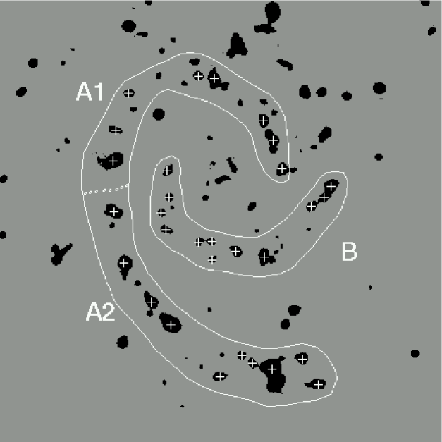
Figure 9: Map of star formation regions in NGC 628. Areas with a surface brightness $\mu({\rm FUV}_{0})<23.63$ mag arcsec^-2 are indicated by black colour. White curves show boundaries of Arms A and B. The dotted line shows the boundary between inner (A1) and outer (A2) parts of Arm A. The white crosses indicate positions of the regions from Table 2. The size of the image is $6.0\times 6.0$ arcmin². North is upward and east is to the left.

Detailed exploration of the size distribution of objects in NGC 628 was made in Elmegreen et al. (2006) in the range of scales from 2 to 110 pc, based on HST images. Elmegreen et al. (2006) found that the cumulative size distribution follows a power law, with slope $\gamma\approx-1.5$. The closest value of the slope of the cumulative size distribution function was found for the star formation regions from the list of Ivanov et al. (1992) that is in the range 30–110 pc. The size distribution of larger objects, H ii regions studied by Hodge (1976), satisfies a power law with slope $\gamma\approx-3.5$ in the range 100–300 pc. The size distribution of complexes of Ivanov et al. (1992) gives $\gamma=-4.1$ in the range 500–1000 pc.

Following Elmegreen et al. (2006), we constructed the cumulative size distribution function for star formation regions in the spiral arms of NGC 628 in the form

$$N(d>D)\propto D^{\gamma},$$

where $N$ is the integrated number of objects that have a diameter $d$ greater than some diameter $D$ (Fig. 10).

The slope of the power law for the size distribution is approximately the same for star formation region populations in both arms as a whole, Arms A and B, and the inner part of Arm A for a size range of 200 to 400 pc, $\gamma\approx-2$ (Table 5). The distribution of the largest regions in both arms as a whole, and Arm A and Arm B separately, satisfies a power law with slope $\gamma\approx-5$. Differences in the size distribution are found between the star formation region populations of the inner and outer parts of Arm A, and between the populations of Arm B and the inner part of Arm A (Fig. 10, Table 5).

Table 5: Mean diameters and size function coefficients.

Arm	$\langle d\rangle^{a}$	$\gamma$	Range	$\gamma$	Range
	(pc)		(pc)		(pc)
A	$400\pm 135$	-1.6	200-400	-4.5	400-650
A1	$360\pm 100$	-2.1	200-300	-2.7	300-600
A2	$435\pm 160$	-0.8	200-400	-3.6	400-650
B	$295\pm 70$	-2.2	200-300	-5.6	300-450
A+B	$360\pm 125$	-2.0	200-400	-4.7	400-650

^a The mean diameters.

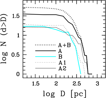
Figure 10: Cumulative size distribution function for the regions in both spiral arms (thick dotted line), Arm A (thick solid line), Arm B (thick grey solid line), the inner part of Arm A (thin dotted line), and the outer part of Arm A (thin solid line).

The size distribution of the star formation region population in Arm B repeats the distribution of the region samples in Arm A with a displacement $\log D\approx 0.2$ (Fig. 10). The size distribution function of the star formation region population in the inner part of Arm A have approximately the same slope in the entire range studied here (Table 5). The size function curves for the populations of Arm B and the inner part of Arm A are very close in the range from 200 to 300 pc, but they vary considerably in the range from 300 to 500 pc. The size distribution function of the star formation regions sample in the outer part of Arm A is characterized by the shallow slope, $\gamma=-0.8$, in the intermediate range from 200 to 400 pc (Table 5).

3.5 Star formation rates within star formation regions

As we pointed out above, the distributions of star formation regions by mass and luminosity and the upper limits of mass and size of regions correlate with the overall star formation rate and depend on properties of interstellar medium. We measured the star formation rates, SFR, and the surface densities of star formation rate, $\Sigma_{\rm SFR}$, within the star formation regions using obtained FUV magnitudes, H$\alpha$ luminosities and sizes. To accomplish this, we adopt the conversion factor of FUV luminosity to star formation rate of Iglesias-Páramo et al. (2006), namely

$${\rm SFR(}M_{\odot}\,{\rm yr^{-1})}=8.13\times 10^{-44}L_{\rm FUV}{\rm(erg\,s^{-1})},$$

in the form

$${\rm SFR(}M_{\odot}\,{\rm yr^{-1})}=7.0\times 10^{-8}\times 10^{-0.4M({\rm FUV})_{\rm c}},$$ (3)

and the conversion factor of H$\alpha$ luminosity to star formation rate of Kennicutt (1998b):

$${\rm SFR(}M_{\odot}\,{\rm yr^{-1})}=7.9\times 10^{-42}L_{{\rm H}\alpha}{\rm(erg\,s^{-1})}.$$ (4)

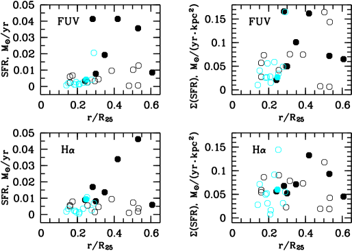
Figure 11: Radial distributions of star formation rate (left panels) and the surface density of star formation rate (right panels) within regions based on their luminosities in FUV (top panels) and H$\alpha$ (bottom panels). Other symbols are the same as in Fig. 2.

The surface densities of star formation rate within the star formation regions are measured as

$$\Sigma_{\rm SFR}={\rm SFR}/S,$$

where SFR and $S$ are obtained from Eqs. (3.4), (3) and (4).

Note that the total star formation rate within studied regions, $\approx 0.25~{}M_{\odot}\,{\rm yr^{-1}}$, is one third of the full SFR in NGC 628 by data of Calzetti et al. (2010), who estimated ${\rm SFR}=0.7\pm 0.2~{}M_{\odot}\,{\rm yr^{-1}}$ in the galaxy as a whole.

Densities of SFR within complexes are typical for star formation regions and comparable to results of Bastian et al. (2005), who found $\Sigma_{\rm SFR}=0.06-0.07~{}M_{\odot}\,{\rm yr^{-1}\,kpc^{-2}}$ for ordinary complexes in M 51. Bright complexes and fainter star formation regions have similar surface densities of star formation rate (Fig. 11).

In spite of the difference in the estimation of SFR(FUV) and SFR(H$\alpha$) for some regions, the results are in agreement with each other, in general, $\langle\Sigma_{\rm SFR}({\rm FUV})\rangle=0.063~{}M_{\odot}\,{\rm yr^{-1}\,kpc^{-2}}$ and $\langle\Sigma_{\rm SFR}({\rm H}\alpha)\rangle=0.061~{}M_{\odot}\,{\rm yr^{-1}\,kpc^{-2}}$. Comparison between SFR(FUV) and SFR(H$\alpha$) of the star formation regions is presented in Fig. 12.

A dependence of SFR density on galactocentic distance is found for objects of Arm A: $\langle\Sigma_{\rm SFR}\rangle\approx 0.07~{}M_{\odot}\,{\rm yr^{-1}\,kpc^{-2}}$ for all regions in Arm A, and only $\approx 0.06~{}M_{\odot}\,{\rm yr^{-1}\,kpc^{-2}}$ for regions with $r/R_{25}<0.32$. The regions in Arm B have a smaller surface density of SFR, on average, than the objects in Arm A, $\langle\Sigma_{\rm SFR}\rangle\approx 0.05~{}M_{\odot}\,{\rm yr^{-1}\,kpc^{-2}}$.

Differences in the density of star formation rate within star formation regions in Arms A and B may indicate differences in interstellar medium parameters between the arms.

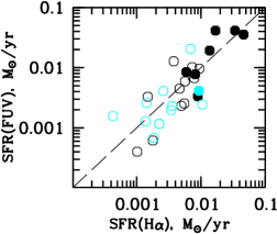
Figure 12: Comparison between SFR(FUV) and SFR(H$\alpha$) of star formation regions. Other symbols are the same as in Fig. 2.

4 Discussion

Spiral density waves can play an important role in asymmetric star formation in spiral arms. Henry, Quillen & Gutermuth (2003) showed on the example of the asymmetry in the spiral arms of M51, that the variable star formation can be caused by more than one spiral density wave. Moreover, an asymmetry in the spiral arms of NGC 628 has been detected in the observed two-dimensional field of radial velocities of the gas in the disc of the galaxy (Sakhibov & Smirnov, 2004). Fourier analysis of the azimuthal distribution of the observed radial velocities in annular (ring) zones at different distances from the centre of the disc shows the existence of two spiral density waves (see Fig. 1a in Sakhibov & Smirnov, 2004), the one-armed wave in addition to the dominant two-armed one. This additional spiral density wave corresponds to the star formation asymmetry in the two main symmetrical arms revealed through the computer-enhanced images of the galaxies by Elmegreen, Elmegreen & Montenegro (1992). In the case of NGC 628, the relatively lower SFR in Arm B can be caused by the asymmetry of the spiral density waves in the galaxy.

In Paper I we assumed that the drastic differences observed between the inner structures located in the spiral arms of NGC 628, one of which hosts the regular chain of large star complexes whereas the other does not, were the result of the existence of a regular magnetic field and the absence of the signature of a shock wave along Arm A. Unfortunately, there are no appropriate magnetic field data for the studied part of NGC 628. The only data concerning the magnetic field were obtained by Heald, Braun & Edmonds (2009) who detected polarized emission at 18 and 22 cm wavelengths from the outer part of the galaxy; their linear beam size was $1.9\times 0.5$ kpc.

The hypothesis proposed in Paper I is not the only possible one. Alternatively, asymmetries in spiral galaxies can be the result of gravitational interactions with another galaxy or galaxies at some point in their history. NGC 628 is a member of a small group of galaxies and its present state may well be the result of close encounters within the group. Close encounters may also trigger episodes of star formation. The same tidal forces that can deform the galaxy may also disrupt giant molecular clouds within the galaxy and induce their gravitational collapse. The numerical simulations of Bottema (2003) show that unbarred grand design galaxies, such as NGC 628, can only be generated by tidal forces resulting from an encounter with other galaxy. However, we believe that tidal interactions could not play a role in the origin of the observed asymmetrical pattern of star formation. It is well established that NGC 628 cannot have undergone any encounter with satellites or other galaxies in the past 1 Gyr (Wakker & van Woerden, 1991; Kamphuis & Briggs, 1992). The spiral filaments are possibly disturbed by interaction with the two large high velocity gas clouds on either side of the disc (Kamphuis & Briggs, 1992; Beckman et al., 2003). However, these high velocity gas clouds are located symmetrically with respect to the centre (Kamphuis & Briggs, 1992). Residual velocity fields of both neutral and ionized gas show the absence of significant velocity deviations from the radial velocity (Kamphuis & Briggs, 1992; Fathi et al., 2007).

In this paper we have found differences in photometric parameters and chemical abundance between the star formation regions in Arms A and B. We suggest that these differences are the result of significant differences in the physical properties of interstellar medium in the opposite arms of NGC 628.

As is known, such physical processes as gravitational collapse and turbulence compression play a key role in creation and evolution of star formation regions over the wide range of scales, from smallest OB associations to largest star complexes (Efremov, 1995; Elmegreen et al., 2000, 2006; Elmegreen, 2002, 2006). The age range of stars within ordinary star formation regions is usually quite small ($\leq 10-15$ Myr) suggesting a coherent star formation mechanism, it separates them from large star complexes which have a much larger intrinsic age spread (Efremov, 1995). This is well illustrated for the young stellar objects in Arm A, where the large complexes are older than the star formation regions ($4.7\pm 1.9$ Myr versus $3.0\pm 2.2$ Myr). We suggest that the difference between photometric ages of star formation regions in Arms A and B is a result of different star formation histories in them. The generation of shock-waves is the source of high pressure in Arm B and probably within the inner part of Arm A (A1). High pressure stimulates formation of dense star formation regions with an active star formation, including formation of massive ($M>10M_{\odot}$) stars (Billett et al., 2002). High pressure from formed H ii regions destroy molecular cloud cores (Elmegreen, 1983). As a result, SFR along Arm B falls for several Myr, star formation regions here do not reach large mass/size, and they have approximately the same photometric ages, $6.0\pm 1.1$ Myr.

The opposite case is observed in Arm A. Pressure along Arm A is lower than along Arm B. As a result, ’doughy’ large complexes are formed here. Initial SFR is low along Arm A; massive stars are not formed immediately. The pressure increase driven by powerful stellar winds from the most massive stars is not high enough to destroy the largest cloud cores. As a result, the young stellar objects here have younger ages with a larger dispersion than the star formation regions in Arm B ($3.7\pm 2.2$ Myr versus $6.0\pm 1.1$ Myr).

Thus, larger star complexes with a lower SFR in the past and a higher SFR now are observed in Arm A, and smaller, more evolved star formation regions are observed in Arm B. This hypothesis is supported by both abundance and photometric data. It is also fully consistent with the findings by Sonbaş et al. (2010), who found nine SNR candidates in NGC 628. Five of them are located in Arm A. Two out of three latest supernovae, SN 2003gd and 2013ej, are also located in Arm A (Fig. 1). Neither SNRs nor supernovae were found in Arm B.

Note that all five SN remnants and two supernovae are located in Arm A between complex A10 found in this work and star formation region a13 (Fig. 1). It is where the star formation complexes and regions with the highest SFRs are observed (see Fig.  11). It is worth noting that SNR 9 and SN 2003gd are located within 10–15 arcsec from our star formation region a13 (Fig. 1). Supernova 2003gd has the normal Type II-P, its progenitor was a red supergiant with initial mass $6-12M_{\odot}$ (van Dyk, Li & Filippenko, 2003; Hendry et al., 2005). The life time of such stars is $\sim 10-50$ Myr. This is consistent with sustained star formation activity during last several tens Myr in this part of the arm.

The same slopes of the luminosity and size distribution functions for the sets of star formation regions in Arms A and B, and the same characteristic separations, $\Lambda\approx 400$ pc (Paper I) of star formation regions in both spiral arms, which depend on fundamental parameters of the medium, show that large scale fundamental properties of interstellar medium and kinematics of the galaxy have no principal differences in Arms A and B.

In spite of the difference between parameters of star formation regions in the central part of Arm A and other parts of the arms, the large scale (2 kpc and more) density of young stellar population along Arms A and B is the same. Masses of star complexes in the central part of Arm A are 3–4 times as much as masses of star formation regions in other parts of Arms A and B (Fig. 3). However, the characteristic separations of star complexes are also 2–4 times as much as separations of star formation regions (Paper I).

We assume that the regular chain of star complexes in Arm A can be explained by presence of the regular magnetic field and absence of the shock wave along the arm only for objects A8–A12 (the first five H ii complexes from the Elmegreens’ chain). In the outer part of Arm A, star formation regions are located more chaotically, the largest star formation complex, A16, is observed here. This complex is the largest and the brightest one in FUV₀ in NGC 628 (Table  3). Parameters of the complex can be related to its location near the corotation radius $R_{\rm cor}$ (Sakhibov & Smirnov (2004) obtained $R_{\rm cor}\approx 7$ kpc or $0.65r/R_{25}$ based on a Fourier analysis of the spatial distribution of radial velocities of the gas in the disc of NGC 628).

5 Conclusions

Photometric properties, chemical abundances and sizes of the 30 brightest star formation regions in the two principal arms of NGC 628 were studied, based on the GALEX ultraviolet, optical $UBVRI$, and H$\alpha$ surface photometry data.

We found, that the star formation regions in one (longer) arm (Arm A) of NGC 628 of are systematically brighter and larger than the regions the other (shorter) arm. However, both luminosity and size distribution functions have approximately the same slopes for the samples of star formation regions in both arms. The star formation regions of Arm A have a higher density of star formation rate than the regions in Arm B. The regions from Arm B show higher N/O ratio at a higher oxygen abundance, but they have lower ultraviolet and H$\alpha$ luminosities. Results of stellar evolutionary synthesis show that the brightest regions in Arm A are younger than the ones in Arm B ($3.7\pm 2.2$ Myr versus $6.0\pm 1.1$ Myr). The star complexes in Arm A are slightly older than the star formation regions ($4.7\pm 1.9$ Myr versus $3.0\pm 2.2$ Myr).

The results can be explained if we suggest that star formation regions in Arm B had higher star formation rate in the past, but now it is lower, than for opposite Arm A.

Our results demonstrate that there is a difference in the inner structures and parameters of the interstellar medium between the two principal spiral arms of NGC 628. In spite of close sizes and spacing of star formation regions in Arm B and in the inner part of Arm A, modern star formation histories in Arms A and B differ. Young stars in the central part of Arm A ($r/R_{25}=0.28-0.42$) are grouping into the large complexes ($d>450$ pc). Smaller star formation regions are absent here.

References

- Aniano et al. (2012) Aniano G. et al., 2012, ApJ, 756, 138
- Artamonov et al. (2010) Artamonov B. P. et al., 2010, Astron. Rep., 54, 1019
- Auld et al. (2006) Auld R. et al., 2006, MNRAS, 371, 1617
- Banse et al. (1983) Banse K., Crane Ph., Ounnas Ch., Ponz D., 1983, MIDAS, in Proc. of DECUS, Zurich, p. 87
- Bastian et al. (2005) Bastian N., Gieles M., Efremov Yu. N., Lamers H. J. G. L. M., 2005, A&A, 443, 79
- Beckman et al. (2003) Beckman J. E., López-Corredoira M. N., Betancort-Rijo J., Castro-Rodríguez N., Cardwell A., 2003, Ap&SS, 284, 747
- Belley & Roy (1992) Belley J., Roy J.-R., 1992, ApJS, 78, 61
- Berg et al. (2013) Berg D. A., Skillman E. D., Garnett D. R., Croxall K. V., Marble A. R., Smith J. D., Gordon K., Kennicutt R. C., Jr., 2013, ApJ, 775, 128
- Bertelli et al. (1994) Bertelli G., Bressan A., Chiosi C., Fagotto F., Nasi E., 1994, A&AS, 106, 275
- Billett et al. (2002) Billett O. H., Hunter D. A., Elmegreen B. G., 2002, AJ, 123, 1454
- Bottema (2003) Bottema R., 2003, MNRAS, 344, 358
- Bresolin et al. (1999) Bresolin F., Kennicutt R. C., Garnett D. R., 1999, ApJ, 510, 104
- Bressan et al. (2012) Bressan A., Marigo P., Girardi L., Salasnich B., Dal Cero C., Rubele S., Nanni A., 2012, MNRAS, 427, 127
- Bruevich et al. (2007) Bruevich V. V., Gusev A. S., Ezhkova O. V., Sakhibov F. Kh., Smirnov M. A., 2007, Astron. Rep., 51, 222
- Calzetti et al. (2010) Calzetti D. et al., 2010, ApJ, 714, 1256
- Cardelli, Clayton & Mathis (1989) Cardelli J. A., Clayton G. C., Mathis J. S., 1989, ApJ, 345, 245
- Cornett et al. (1994) Cornett R. H. et al., 1994, ApJ, 426, 553
- de Grijs et al. (2003) de Grijs R., Anders P., Bastian N., Lynds R., Lamers H. J. G. L. M., O’Neil E. J., 2003, MNRAS, 343, 1285
- de la Fuente Marcos & de la Fuente Marcos (2009) de la Fuente Marcos R., de la Fuente Marcos C., 2009, ApJ, 700, 436
- Dolphin & Kennicutt (2002) Dolphin A. E., Kennicutt R. C. Jr., 2002, AJ, 123, 207
- Efremov (1978) Efremov Yu. N., 1978, Sov. Astron. Lett., 4, 66
- Efremov (1979) Efremov Yu. N., 1979, Sov. Astron. Lett., 5, 12
- Efremov (1989) Efremov Yu. N., 1989, Sites of Star Formation in Galaxies: Star Complexes and Spiral Arms. Fizmatlit, Moscow, p. 246 (in Russian)
- Efremov (1995) Efremov Yu. N., 1995, AJ, 110, 2757
- Efremov & Elmegreen (1998) Efremov Yu. N., Elmegreen B. G., 1998, MNRAS, 299, 588
- Egorov, Lozinskaya & Moiseev (2013) Egorov O. V., Lozinskaya T. A., Moiseev A. V., 2013, MNRAS, 429, 1450
- Elmegreen (1983) Elmegreen B. G., 1983, MNRAS, 203, 1011
- Elmegreen (1994) Elmegreen B. G., 1994, ApJ, 433, 39
- Elmegreen (2002) Elmegreen B. G., 2002, ApJ, 564, 773
- Elmegreen (2006) Elmegreen B. G., 2006, in Del Toro Iniesta J. C. et al., eds, The Many Scales in the Universe: JENAM 2004 Astrophysics Reviews. Springer, Dordrecht, p. 99
- Elmegreen (2009) Elmegreen B. G., 2009, in Andersen J., Bland-Hawthorn J., Nordström B., eds, Proc. IAU Symp. 254, The Galaxy Disk in Cosmological Context. Kluwer, Dordrecht, p. 289
- Elmegreen & Efremov (1996) Elmegreen B. G., Efremov Yu. N., 1996, ApJ, 466, 802
- Elmegreen & Efremov (1997) Elmegreen B. G., Efremov Yu. N., 1997, ApJ, 480, 235
- Elmegreen & Elmegreen (1983) Elmegreen B. G., Elmegreen D. M., 1983, MNRAS, 203, 31
- Elmegreen & Lada (1977) Elmegreen B. G., Lada C. J., 1977, ApJ, 214, 725
- Elmegreen, Elmegreen & Montenegro (1992) Elmegreen B. G., Elmegreen D. M., Montenegro L., 1992, ApJS, 79, 37
- Elmegreen et al. (2000) Elmegreen B. G., Efremov Y., Pudritz R. E., Zinnecker H., 2000, in Mannings V., Boss A. P., Russell S. S., eds, Protostars and Planets IV. University of Arizona Press, Tucson, p. 179
- Elmegreen et al. (2006) Elmegreen B. G., Elmegreen D. M., Chandar R., Whitmore B., Regan M., 2006, ApJ, 644, 879
- Fathi et al. (2007) Fathi K., Beckman J. E., Zurita A., Relaño M., Knapen J. H., Daigle O., Hernandez O., Carignan C., 2007, A&A, 466, 905
- Ferguson et al. (1998) Ferguson A. M. N., Gallagher J. S., Wyse R. F. G., 1998, AJ, 116, 673
- Gieles et al. (2006) Gieles M., Larsen S. S., Bastian N., Stein I. T., 2006, A&A, 450, 129
- Girardi et al. (2000) Girardi L., Bressan A., Bertelli G., Chiosi C., 2000, A&AS, 141, 371
- Grøsbol & Ponz (1990) Grøsbol P. J., Ponz J. D., 1990, The MIDAS System, in Longo G. and Sedmak G., eds, Acquisition, Processing and Archiving of Astronomical Images, OAC and FORMEZ, p. 109
- Gusev & Efremov (2013) Gusev A. S., Efremov Yu. N., 2013, MNRAS, 434, 313 (Paper I)
- Gusev & Park (2003) Gusev A. S., Park M.-G., 2003, A&A, 410, 117
- Gusev et al. (2012) Gusev A. S., Pilyugin L. S., Sakhibov F., Dodonov S. N., Ezhkova O. V., Khramtsova M. S., 2012, MNRAS, 424, 1930
- Haas et al. (2008) Haas M. R., Gieles M., Scheepmaker R. A., Larsen S. S., Lamers H. J. G. L. M., 2008, A&A, 487, 937
- Heald, Braun & Edmonds (2009) Heald G., Braun R., Edmonds R., 2009, A&A, 503, 409
- Hendry et al. (2005) Hendry M. A. et al., 2005, MNRAS, 359, 906
- Henry, Quillen & Gutermuth (2003) Henry A. L., Quillen A. C., Gutermuth R., 2003, AJ, 126, 2831
- Herrmann et al. (2008) Herrmann K. A., Ciardullo R., Feldmeier J. J., Vinciguerra M., 2008, ApJ, 683, 630
- Hodge (1976) Hodge P. W., 1976, ApJ, 205, 728
- Iglesias-Páramo et al. (2006) Iglesias-Páramo J. et al., 2006, ApJS, 164, 38
- Ivanov et al. (1992) Ivanov G. R., Popravko G., Efremov Yu. N., Tichonov N. A., Karachentsev I. D., 1992, A&AS, 96, 645
- Kamphuis & Briggs (1992) Kamphuis J., Briggs F., 1992, A&A, 253, 335
- Kennicutt (1998a) Kennicutt R. C., 1998a, ApJ, 498, 541
- Kennicutt (1998b) Kennicutt R. C., 1998b, ARA&A, 36, 189
- Kennicutt & Hodge (1976) Kennicutt R. C., Hodge P. W., 1976, ApJ, 207, 36
- Kewley & Ellison (2008) Kewley L. J., Ellison S. L., 2008, ApJ, 681, 1183
- Kewley et al. (2006) Kewley L. J., Groves B., Kauffmann G., Heckman T., 2006, MNRAS, 372, 961
- Kharchenko et al. (2009) Kharchenko N. V., Piskunov A. E., Röser S., Schilbach E., Scholz R.-D., Zinnecker H., 2009, A&A, 504, 681
- Kobulnicky & Kewley (2004) Kobulnicky H. A., Kewley L. J., 2004, ApJ, 617, 240
- Larsen (2002) Larsen S. S., 2002, AJ, 124, 1393
- Larsen et al. (2011) Larsen S. S. et al., 2011, A&A, 532, A147
- Levesque, Kewley & Larson (2010) Levesque E. M., Kewley L. J., Larson K. L., 2010, AJ, 139, 712
- López-Sánchez et al. (2012) López-Sánchez Á. R., Dopita M. A., Kewley L. J., Zahid H. J., Nicholls D. C., Scharwächter J., 2012, MNRAS, 426, 2630
- Mallery et al. (2007) Mallery R. P. et al., 2007, ApJS, 173, 482
- Marigo & Girardi (2007) Marigo P., Girardi L., 2007, A&A, 469, 239
- Marigo et al. (2008) Marigo P., Girardi L., Bressan A., Groenewegen M. A. T., Silva L., Granato G. L., 2008, A&A, 482, 883
- McCall et al. (1985) McCall M. L., Rybski P. M., Shields G. A., 1985, ApJS, 57, 1
- Mollá & Gavilán (2010) Mollá M., Gavilán M., 2010, Mem. S. A. It, 81, 992
- Mollá et al. (2006) Mollá M., Vílchez J. M., Gavilán M., Díaz A. I., 2006, MNRAS, 372, 1069
- Mora et al. (2009) Mora M. D., Larsen S. S., Kissler-Patig M., Brodie J. P., Richtler T., 2009, A&A, 501, 949
- Morrissey et al. (2005) Morrissey P. et al., 2005, ApJ, 619, L7
- Moustakas et al. (2010) Moustakas J., Kennicutt R. C., Jr., Tremonti C. A., Dale D. A., Smith J.-D. T., Calzetti D., 2010, ApJS, 190, 233
- Odekon (2008) Odekon M. C., 2008, ApJ, 681, 1248
- Olivares et al. (2010) Olivares E. F. et al., 2010, ApJ, 715, 833
- Paturel et al. (2003) Paturel G., Petit C., Prugniel Ph., Theureau G., Rousseau J., Brouty M., Dubois P., Cambresy L., 2003, A&A, 412, 45
- Pettini & Pagel (2004) Pettini M., Pagel B., 2004, MNRAS, 348, L59
- Pilyugin & Mattsson (2011) Pilyugin L. S., Mattsson L., 2011, MNRAS, 412, 1145
- Pilyugin & Thuan (2005) Pilyugin L. S., Thuan T. X., 2005, ApJ, 631, 231
- Pilyugin, Vílchez & Thuan (2010) Pilyugin L. S., Vílchez J. M., Thuan T. X., 2010, ApJ, 720, 1738
- Piskunov et al. (2009) Piskunov A. E., Kharchenko N. V., Schilbach E., Röser S., Scholz R.-D., Zinnecker H., 2009, A&A, 507, L5
- Rosales-Ortega et al. (2011) Rosales-Ortega F. F., Diaz A. I., Kennicutt R. C., Sanchez S. F., 2011, MNRAS, 415, 2439
- Sakhibov & Smirnov (2004) Sakhibov F. Kh., Smirnov M. A., 2004, Astron. Rep. 48, 995
- Schlafly & Finkbeiner (2011) Schlafly E. F., Finkbeiner D. P., 2011, ApJ, 737, 103
- Sharina et al. (1996) Sharina M. E., Karachentsev I. D., Tikhonov N. A., 1996, A&AS, 119, 499
- Sonbaş et al. (2010) Sonbaş E., Akyüz A., Balman Ş., Özel M. E., 2010, A&A, 517, A91
- van den Bergh & Lafontaine (1984) van den Bergh S., Lafontaine A., 1984, AJ, 89, 1822
- van Dyk, Li & Filippenko (2003) van Dyk S. D., Li W., Filippenko A. V., 2003, PASP, 115, 1289
- van Dyk et al. (2006) van Dyk S. D., Li W., Filippenko A. V., 2006, PASP, 118, 351
- Villa-Costas & Edmunds (1993) Villa-Costas M. B., Edmunds M. G., 1993, MNRAS, 265, 199
- Wakker & van Woerden (1991) Wakker B. P., van Woerden H., 1991, A&A, 250, 509
- Whitmore et al. (1999) Whitmore B. C., Zhang Q., Leitherer C., Fall S. M., Schweizer F., Miller B. W., 1999, AJ, 118, 1551
- Wyder et al. (2007) Wyder T. K. et al., 2007, ApJS, 173, 293
- Zasov & Bizyaev (1996) Zasov A. V., Bizyaev D. V., 1996, Astron. Lett., 22, 71
- Zepf et al. (1999) Zepf S. E., Ashman K. M. English J., Freeman K. C., Sharples R. M., 1999, AJ, 118, 752