High order time–splitting methods for irreversible equations

Abstract

In this work, high order splitting methods of integration without negative steps are shown which can be used in irreversible problems, like reaction–difussion or complex Guinzburg–Landau equations. The methods consist in a suitable affine combinations of Lie–Tortter schemes with different positive steps. The number of basic steps for these methods grows quadratically with the order, while for symplectic methods, the growth is exponential. Furthermore, the calculations can be performed in parallel, so that the computation time can be significantly reduced using multiple processors. Convergence results of these methods are proved for a large kind of semilinear problems, that includes reaction-difussion systems and dissipative perturbation of Hamiltonian systems. splitting methods, irreversible dynamics, high order method
AMS Subject Classification: 65M12, 35Q56, 35K57

1 Introduction

The goal of the present article is to derive arbitrary order splitting integrators for irreversible problems. We are mainly interested in dissipative pseudo-differentiable problems which cannot be solved neither by lines methods nor by usual splitting integrators with negative steps. In order to avoid negative steps, symplectic methods with complex steps are proposed in the literature, but in this case analytic properties on the operators are required. These assumptions on the operators restrict the application of this kind of methods to reaction–diffusion type problems.

In this article we obtain integrators that, at the same time, avoid the use of negative steps and do not require special assumptions on the operator, as well as they exploit the simplicity of the decomposition of the original problem. These methods can also be applied to problems with nonlocal nonlinearities as it is shown below. It is possible to build arbitrary high order integrators for which the number of basic steps is lower than previous symplectic methods. Moreover, these methods can naturally be parallelized. In this work, we present a rigorous proof of the convergence of the proposed methods, and we also test their performance in several examples of interest.

We study the initial value problem

$$\begin{cases}\partial_{t}u=A_{0}\,u+A_{1}(u),\\ u(0)=u_{0},\end{cases}$$ (1.1)

where $A_{0}$ is a linear closed operator densely defined in $D(A_{0})\subset\mathsf{H}$, $\mathsf{H}$ is a Hilbert space, which generates a quasicontraction semi-group of operators. We assume that the nonlinear term $A_{1}:\mathsf{H}\to\mathsf{H}$ is a smooth mapping with $A_{1}(0)=0$. In many problems of interest, the partial equations

$$\partial_{t}u= \,A_{0}\,u,$$ (1.2a)

$$\partial_{t}u= \,A_{1}(u),$$ (1.2b)

can be easily solved either analytically or numerically, which enable to find approximated solutions of the problem (1.1) applying in turn the flows $\phi_{0}$ and $\phi_{1}$ associated to each partial problem (1.2a) and (1.2b) respectively.

There exist many numerical integration methods for (1.1) based on splitting methods, the most known are the Lie–Trotter and Strang methods defined by

$$\Phi_{\mathrm{Lie}}(h,u)= \,\phi_{1}(h,\phi_{0}(h,u)),$$

$$\Phi_{\mathrm{Strang}}(h,u)= \,\phi_{0}(h/2,\phi_{1}(h,\phi_{0}(h/2,u))),$$

where $h$ is the time step of the numerical integration. It can be proved that $\Phi_{\mathrm{Lie}}$ has order $1$ and $\Phi_{\mathrm{Strang}}$ has order $2$, where the order $q$ represents the greatest natural number such that the truncation error between the real flow $\phi$ of the equation (1.1) and the numerical method $\Phi$ satisfies

$$\|\phi(h,u)-\Phi(h,u)\|_{\mathsf{H}}\leq C(u)h^{q+1}$$

for $0<h<h_{*}$.

A highly known example of problem (1.1) is the nonlinear Schrödinger equation (NLS)

$$\partial_{t}u=\mathrm{i}\Delta u+\mathrm{i}|u|^{2}u,$$ (1.3)

where the partial flows associated to each term of the equation are given by

$$\phi_{0}(t,u)= \,\exp(\mathrm{i}t\Delta)u,$$

$$\phi_{1}(t,u)= \,\exp(\mathrm{i}t|u|^{2})u,$$

which represent the evolution of a free particle and self–phase modulation respectively. This is not exactly the problem we are interested in solving since $A_{0}$ generates a strongly continuous group of operators, that is we are in the presence of a reversible system. In [21], [19] and [24], the authors present numerical integrators for Hamiltonian systems of order $q=3,4,2n$ respectively, which are known as symplectic integrators. The general form of this methods is the following:

$$\Phi_{Sym}(h)=\phi_{1}(b_{m}h)\circ\phi_{0}(a_{m}h)\circ\cdots\circ\phi_{1}(b_{1}h)\circ\phi_{0}(a_{1}h),$$ (1.4)

with $a_{1}+\cdots+a_{m}=b_{1}+\cdots+b_{m}=1$. In the pioneering work [21], a symplectic operator $\Phi_{Sym}$ of order $3$ is presented, taking $a_{1}=7/24$, $a_{2}=3/4$, $a_{3}=-1/24$ and $b_{1}=2/3$, $b_{2}=-2/3$, $b_{3}=1$. In [19] a symplectic operator of order $4$ is considered, where

$$a_{1}= \,a_{4}=\frac{1}{2(2-2^{1/3})},\;a_{2}=a_{3}=-\frac{2^{1/3}-1}{2(2-2^{1/3})},$$

$$b_{1}= \,b_{3}=\frac{1}{2-2^{1/3}},\;b_{2}=-\frac{2^{1/3}}{2-2^{1/3}},\;b_{4}=0.$$

In [24], Yoshida presents a systematic way to obtain integrators of arbitrary even order, based on the Baker–Campbell–Hausdorff formula. These integrators can be set inductively

$$\Phi_{Sym,2n+2}(h)=\Phi_{Sym,2n}(z_{1}h)\circ\Phi_{Sym,2n}(z_{0}h)\circ\Phi_{Sym,2n}(z_{1}h),$$

with $z_{0}+2z_{1}=1$ and $z_{0}^{2n+1}+z_{1}^{2n+1}=0$. The total number of steps of the method of order $q=2n$ is $S_{T}=3^{n}$. Nevertheless, for order $q=6,8$ there can be shown symplectic integrators with $8$ and $16$ steps respectively.

In the last years, many authors started the rigorous study of the convergence of the symplectic methods applied to Hamiltonian systems in infinite dimension. In [5] the NLS problem given by (1.3) in dimension $2$ is considered and it is proved the convergence of the Lie–Trotter and Strang methods in $L^{2}(\mathbb{R}^{2})$ with order $1$ and $2$ respectively (see also [11] and [12]). In [18] and [13] similar results are proved for the Gross–Pitaevskii equation given by:

$$\mathrm{i}\partial_{t}u=-\Delta u+|x|^{2}u+|u|^{2}u,$$

In both cases, the solutions are needed to be differentiable with respect to time, and therefore initial data in $D(A_{0}^{k})$ is considered, where $A_{0}$ is the corresponding differential operator.

The symplectic methods with order $q>2$ require some step to be negative (see [14]), inhibiting its application to irreversible problems. In [7], the authors develop splitting methods for irreversible problems, that use complex time steps having positive real part: going to the complex plane allows to considerably increase the accuracy, while keeping small time steps. The total number of steps using the so called triple jump method of order $q=2n$ is $S_{T}=3^{n-1}$ for order not greater than $8$ and for the quadruple jump method is $S_{T}=4\times 3^{n-2}$ for order not greater than $12$. Finally we recall that the rigorous approach given in this article is based upon the results for linear operators given in [16] while the nonlinear problem is only formally discussed.

Since our interest is focused on irreversible pseudo–differential problems, the paradigmatic example we have in mind is the regularized cubic Schrödinger equation:

$$\partial_{t}u=\mathrm{i}\Delta u-(-\Delta)^{\beta}u+\mathrm{i}|u|^{2}u,$$ (1.5)

where $0<\beta<1$. It is natural to split the problem into the linear equation $\partial_{t}u=\mathrm{i}\Delta u-(-\Delta)^{\beta}u$ and the ordinary differential equation system given by $\dot{u}=\mathrm{i}|u|^{2}u$, where the linear problem is ill-posed for negative times. Note that the same procedure can be applied to nonlocal nonlinearities like convolution potentials as it is done in example 4.3 below (see also example 4.1 in [6]). Since $\mathrm{i}\Delta-(-\Delta)^{\beta}$ is a pseudo–differential operator, it can not be discretized in space in order to use some method of lines, as Runge–Kutta schemes. Observe that the strongly continuous semigroup generated by the linear part of equation (1.5) can not be extended to an open sector $\{z\in\mathbb{C}:|\arg(z)|<\theta\}$ since its spectrum is $\{-\mathrm{i}\lambda-\lambda^{\beta}:\lambda\geq 0\}\not\subseteq\{\lambda\in\mathbb{C}:\mathrm{arg}|\lambda-\omega|\geq\pi/2+\theta\}$ for any $\omega\in\mathbb{R}$, contrary to Hille–Yosida–Phillips theorem (see [20], theorem X.47b). Therefore, splitting methods with complex times described in [7] can not be used. The case $\beta=1$ corresponds to the complex Ginzburg–Landau equation (see [4] and references there):

$$\partial_{t}u=a\Delta u+b|u|^{2}u,$$ (1.6)

where $a,b\in\mathbb{C}$ with $\mathrm{Re}(a)>0$. The spectrum of the operator $a\Delta$ is $\sigma(a\Delta)=\{-a\lambda:\lambda\geq 0\}$ and generates a strongly continuous semi-group on the open sector $\{z\in\mathbb{C}:|\arg(z)|<\pi/2-|\arg(a)|\}$. In [7], it is shown that the arguments of the complex steps grow with the order of the method, exceeding the value $\pi/2-|\arg(a)|$ for order high enough. Therefore, among integrators proposed in [7], only the low-order methods can be used.

In this work, we present a family of splitting type methods for arbitrary order with positive time step, that exploit the simplicity of the partial flows in non reversible problems. Here we describe the methods proposed: given the associated flows $\phi_{0},\phi_{1}$ of the partial problems, we define the maps $\Phi^{+}(h)=\phi_{1}(h)\circ\phi_{0}(h)$, $\Phi^{-}(h)=\phi_{0}(h)\circ\phi_{1}(h)$ and $\Phi_{m}^{\pm}(h)=\Phi^{\pm}(h)\circ\Phi_{m-1}^{\pm}(h)$ with $\Phi_{1}^{\pm}=\Phi^{\pm}$, and consider the following methods:

$$\Phi(h)= \,\sum_{m=1}^{s}\gamma_{m}\Phi_{m}^{\pm}(h/m)$$ (asymmetric), (1.7a)

$$\Phi(h)= \,\sum_{m=1}^{s}\gamma_{m}(\Phi_{m}^{+}(h/m)+\Phi_{m}^{-}(h/m))$$ (symmetric) . (1.7b)

We will show below that under appropriated assumptions, the integrators given by (1.7a) and (1.7b) are convergent with order $q$, if $\gamma=(\gamma_{1},\ldots,\gamma_{s})$ satisfies the following conditions

$$\begin{split}1=&\,\gamma_{1}+\gamma_{2}+\cdots+\gamma_{s},\\ 0=&\,\gamma_{1}+2^{-k}\gamma_{2}+\cdots+s^{-k}\gamma_{s},\quad 1\leq k\leq q-1,\end{split}$$ (1.8a)

$$\begin{split}\frac{1}{2}=&\,\gamma_{1}+\gamma_{2}+\cdots+\gamma_{s},\\ 0=&\,\gamma_{1}+2^{-2k}\gamma_{2}+\cdots+s^{-2k}\gamma_{s},\quad 1\leq k\leq n-1,\end{split}$$ (1.8b)

respectively, where $2n=q$. The first method (1.7a) is the $h$-extrapolation of the first order Lie–Trotter splitting method and the second method (1.7b) is the $h^{2}$-extrapolation of the symmetrization of this method. The general extrapolation technique is described in [15] and an application of these techniques applied to classical Hamiltonian systems is shown in [9].

The possibility of computing $\Phi_{m}^{\pm}$ simultaneously, allows to reduce significantly the total time of computation using multiple processors. The total number of steps for (1.7a) is given by $S_{T}=2\sum_{\gamma_{m}\neq 0}m$ and $S_{T}=4\sum_{\gamma_{m}\neq 0}m$ for (1.7b). Neglecting the communication time between the processors, the total time of computation working in parallel, turns out to be proportional to $S_{P}=2\max\limits_{\gamma_{m}\neq 0}m$ in both cases. The system (1.8a) has solution for $s\geq q$, and hence there exist methods of arbitrary order $q$ with $S_{P}=2q$ and $S_{T}=q(q+1)$. On the other side, the system (1.8b) has solution for $s\geq n$, which shows that there exist integrators of arbitrary even order $q=2n$ with $S_{P}=q$ and $S_{T}=q(q/2+1)$, using the double of processors. As it can be seen the minimum number of steps working in parallel for the symmetric method is smaller than the corresponding one for the asymmetric method. Also, in the examples considered below, the symmetric method presents less error than the asymmetric method. These two latter issues pointed out justify the choice of the symmetric method over the asymmetric one. Even using one single processor, the total number of steps grows quadratically with the order, while both methods presented in [24] and [7] have an exponential growth.

The paper is organized as follows: In section 2 we give the basic definitions and preliminary results. We define the stability and uniform stability bounds for an application which extend the logarithmic norm notion given in [10]. Following the ideas of [5], [18] and [13], we consider a decreasing sequence of dense subspaces where the flows are repeatedly differentiable. In section 3 we prove consistency and stability results for the methods (1.7), from where we deduce the convergence in the standard way. In section 4 we give several examples of the application of the methods to initial value problems for ODE’s and irreversible PDE’s.

2 Notation and preliminary results

From now on, we will denote $\phi$ the flow of the equation (1.1), $\phi_{0}$ and $\phi_{1}$ the flows associated to the respective partial problems $\eqref{eq: ut=A0u}$ and $\eqref{eq: ut=A1u}$. Also, we will write $\Phi^{\pm}$ the maps defined by $\Phi^{+}(h)=\phi_{1}(h)\circ\phi_{0}(h)$, $\Phi^{-}(h)=\phi_{0}(h)\circ\phi_{1}(h)$ and $\Phi_{m}^{\pm}(h)=\Phi^{\pm}(h)\circ\Phi_{m-1}^{\pm}(h)$ with $\Phi_{1}^{\pm}=\Phi^{\pm}$. Finally, we will use the letter $\Phi$ for the numerical integrators given by (1.7a) and (1.7b).

In the next subsections we will give some preliminary results which will be used in section 3. Subsection 2.1 provides combinatorial results necessary to prove the consistency in subsection 3.1. The proof of stability given in subsection 3.2 requires the results for stable maps proved in subsection 2.2. In order to prove theorems 3.1 and 3.2 we establish the concept of compatible flows given in subsection 2.3.

2.1 Combinatorial results

For a multiindex $\beta=(\beta_{1},\ldots,\beta_{r})\in\mathbb{N}^{r}$, we define $\beta!=\beta_{1}!\ldots\beta_{r}!$ and $I_{r,k}=\{\beta\in\mathbb{N}^{r}:\beta_{1}+\cdots+\beta_{r}=k\}$ which satisfy $\mathbb{N}^{r}=\bigcup_{k=1}^{\infty}I_{r,k}$.

Remark 2.1.

It holds $I_{r,k}=\emptyset$ if $r>k$, $I_{k,k}=\{(1,\ldots,1)\}$ and for $r+s\leq k$, $I_{r+s,k}=\bigcup_{j=s}^{k-r}I_{r,k-j}\times I_{s,j}$.

We will need the following lemmas. We will give an outline of the proof of the first lemma and skip the proof of the second one.

Lemma 2.2.

Let $q\in\mathbb{N}$, if $\gamma=(\gamma_{1},\ldots,\gamma_{s})$ satisfies the conditions (1.8a), then for $1\leq k\leq q$, it holds that

$$\sum_{m=r}^{s}\binom{m}{r}m^{-k}\gamma_{m}= \,0,\qquad r=1,\ldots,k-1,$$

$$\sum_{m=k}^{s}\binom{m}{k}m^{-k}\gamma_{m}= \,\frac{1}{k!}.$$

Proof.

We consider the falling factorial $(x)_{k}=x(x-1)\dots(x-k+1)$, which is a monic polynomial of degree $k$ such that $(x)_{k}=\sum_{j=0}^{k}S(k,j)x^{j}.$ Then, for any natural number $m$ satisfying $0\leq m\leq k-1$, we have that $(m)_{k}=0$ and therefore $\sum_{j=0}^{k}S(k,j)m^{j}=0.$ For the second equality we use that for $1\leq r\leq k-1$

$$\sum_{m=r}^{s}\binom{m}{r}m^{-k}\gamma_{m}=\frac{1}{r!}\sum_{m=r}^{s}(m)_{r}m^{-k}\gamma_{m}=-\frac{1}{r!}\sum_{m=1}^{r-1}\sum_{j=0}^{r}S(r,j)m^{j}\frac{\gamma_{m}}{m^{k}}=0$$

where we have used the hypothesis on the second equality. Analogously for the first equality we have:

$$k!\sum_{m=k}^{s}\binom{m}{k}m^{-k}\gamma_{m}=\sum_{m=k}^{s}(m)_{k}m^{-k}\gamma_{m}=1-\sum_{m=1}^{k-1}\left(\frac{\sum_{j=0}^{k}S(k,j)m^{j}}{m^{k}}\right)\gamma_{m}=1$$

where we have used the hypothesis on the second equality. ∎

Lemma 2.3.

Let $n\in\mathbb{N}$, if $\gamma=(\gamma_{1},\ldots,\gamma_{s})$ satisfies the conditions (1.8b), then for $1\leq k\leq q=2n$, it holds that

$$\sum_{m=1}^{s}\left[\binom{m}{r}+(-1)^{k+r}\binom{m+r-1}{m-1}\right]m^{-k}\gamma_{m}= \,0,\quad r=1,\ldots,k-1,$$

$$\sum_{m=1}^{s}\left[\binom{m}{k}+\binom{m+k-1}{m-1}\right]m^{-k}\gamma_{m}= \,\frac{1}{k!}.$$

Proof.

The proof is similar to the previous lemma. ∎

2.2 Stable maps

Let $\mathsf{H}$ be a Hilbert space, and $\varphi:\mathbb{R}_{+}\times\mathsf{H}\to\mathsf{H}$ a continuous map such that $\varphi(h)=\varphi(h,\cdot):\mathsf{H}\to\mathsf{H}$ is Lipschitz continuous and $\varphi(0)=I$, we define

$$\Lambda(\varphi,h)=\mathop{\sup_{u,u^{\prime}\in\mathsf{H}}}_{u\neq u^{\prime}}\frac{\|\varphi(h,u)-\varphi(h,u^{\prime})\|_{\mathsf{H}}}{\|u-u^{\prime}\|_{\mathsf{H}}}.$$

We say that $\varphi$ is stable if $\kappa(\varphi)=\limsup_{h\downarrow 0}h^{-1}(\Lambda(\varphi,h)-1)<\infty$. For any $\kappa>\kappa(\varphi)$, there exists $h^{*}(\kappa)>0$ such that

$$\Lambda(\varphi,h)\leq 1+\kappa h\leq\mathrm{e}^{\kappa h},$$

if $0<h<h_{*}=h_{*}(\kappa)$. For $\varphi$ a linear flow, $\kappa(\varphi)$ is the logarithmic norm of the generator (see [10]). A map $\varphi$ is called uniformly stable if

$$\mu(\varphi)=\limsup_{h\downarrow 0}h^{-1}\Lambda(\varphi-I,h)<\infty.$$

Since $\Lambda(\varphi,h)\leq 1+\Lambda(\varphi-I,h)$, uniform stability implies stability. Observe that the family of (uniformly) stable maps is scale-invariant and if $\varphi_{\lambda}(h,u):=\varphi(\lambda h,u)$ with $\lambda>0$, then $\kappa(\varphi_{\lambda})=\lambda\kappa(\varphi)$, $\mu(\varphi_{\lambda})=\lambda\mu(\varphi)$. If $\varphi$ is a quasicontraction semi-group then $\varphi$ is stable but it is uniformly stable if and only if the infinitesimal generator is a bounded operator.

Proposition 2.4.

If $\phi_{0},\phi_{1}$ are (uniformly) stable, then the map $\varphi$ defined by $\varphi(h,u)=\phi_{0}(h,\phi_{1}(h,u))$, is (uniformly) stable and $\kappa(\varphi)\leq\kappa(\phi_{0})+\kappa(\phi_{1})$ ($\mu(\varphi)\leq\mu(\phi_{0})+\mu(\phi_{1})$).

Proof.

Since $\Lambda(\varphi,h)\leq\Lambda(\phi_{0},h)\Lambda(\phi_{1},h)$, it follows that

$$\frac{\Lambda(\varphi,h)-1}{h}\leq\frac{\Lambda(\phi_{0},h)-1}{h}+\Lambda(\phi_{0},h)\frac{\Lambda(\phi_{1},h)-1}{h},$$

using that $\Lambda(\phi_{0},h)\to 1$, we get the stability. Writing $\varphi-I=(\phi_{0}-I)\circ\phi_{1}+\phi_{1}-I$, we have

$$\Lambda(\varphi-I,h)\leq\Lambda(\phi_{0}-I,h)\Lambda(\phi_{1},h)+\Lambda(\phi_{1}-I,h).$$

and then $\mu(\varphi)\leq\mu(\phi_{0})+\mu(\phi_{1})$. ∎

Let $\{\Phi_{m}\}_{1\leq m\leq s}$ be a family of stable maps and $\Phi$ an affine combination, i.e. $\Phi=\gamma_{1}\Phi_{1}+\cdots+\gamma_{s}\Phi_{s}$ with $\gamma_{1}+\cdots+\gamma_{s}=1$, it is easy to see that

$$\Lambda(\Phi,h)\leq\sum_{m=1}^{s}|\gamma_{m}|\Lambda(\Phi_{m},h),$$

therefore, $\Phi$ is not necessarily a stable map (but it is true for convex combinations). We have

Proposition 2.5.

If $\{\Phi_{m}\}_{1\leq m\leq s}$ is a family of uniformly stable maps, then an affine combination $\Phi$ is uniformly stable.

Proof.

Writing $I=\gamma_{1}I+\cdots+\gamma_{s}I$ and $\Phi-I=\gamma_{1}(\Phi_{1}-I)+\cdots+\gamma_{s}(\Phi_{s}-I)$, therefore we get $\mu(\Phi)\leq\sum_{1\leq m\leq s}|\gamma_{m}|\mu(\Phi_{m})$. ∎

2.3 Compatible flows

Let $\{\mathsf{H}_{k}\}_{k\geq 0}$ be a sequence of Hilbert spaces satisfying $\mathsf{H}_{k+1}\hookrightarrow\mathsf{H}_{k}$, we define for $k\geq 0$

$$\mathcal{D}_{k}=\{f\in C^{\infty}(\mathsf{H}_{k},\mathsf{H}_{0}):\left.f\right|_{H_{k+l}}\in C^{\infty}(\mathsf{H}_{k+l},\mathsf{H}_{l})\text{ for all }l\geq 0\}.$$

We can see that if $f\in\mathcal{D}_{k}$ and $g\in\mathcal{D}_{j}$, then $f\circ g\in\mathcal{D}_{j+k}$. Let $\varphi\in C([0,h_{*})\times\mathsf{H}_{0},\mathsf{H}_{0})$, we say that $\varphi$ is compatible with $\{\mathsf{H}_{k}\}_{k\geq 0}$ if and only if for $l,k\geq 0$, $\varphi\in C^{k,\infty}([0,h_{*})\times\mathsf{H}_{k+l},\mathsf{H}_{l})$. As an example, let $A:D(A)\to\mathsf{H}$ be a self–adjoint operator, if we take $\mathsf{H}_{k}=D(A^{k})$ with the inner product $\langle u,v\rangle_{\mathsf{H}_{k}}=\langle u,v\rangle_{\mathsf{H}}+\langle A^{k}u,A^{k}v\rangle_{\mathsf{H}}$, we see that $A^{k}\in\mathcal{D}_{k}$. Assume $\varphi$ is the unitary group with infinitesimal generator $iA$, we have $\varphi$ is compatible with $\{\mathsf{H}_{k}\}_{k\geq 0}$ and

$$\frac{\partial^{k}}{\partial h^{k}}\varphi(h,u)=\varphi(h,(iA)^{k}u).$$

Let $f\in\mathcal{D}_{j}$ and $\varphi$ compatible with $\{\mathsf{H}_{k}\}$, we have $f\circ\varphi\in C^{k,\infty}([0,h_{*})\times\mathsf{H}_{j+k+l},\mathsf{H}_{l})$. Then we define the linear operator $L_{k}[\varphi]:\mathcal{D}_{j}\to\mathcal{D}_{j+k}$ as

$$(L_{k}[\varphi]f)(u)=\left.\frac{\partial^{k}}{\partial h^{k}}f(\varphi(h,u))\right|_{h=0},$$

with $u\in\mathsf{H}_{j+k}$.

Lemma 2.6.

If $\varphi$ and $\psi$ are compatible with $\{\mathsf{H}_{k}\}_{k\geq 0}$, then $\varphi\circ\psi$ also is compatible with $\{\mathsf{H}_{k}\}_{k\geq 0}$ and satisfies

$$L_{k}[\varphi\circ\psi]=\sum_{j=0}^{k}\binom{k}{j}L_{k-j}[\psi]L_{j}[\varphi].$$

Proof.

Let $\theta(\tau,\eta,u)=\varphi(\tau,\psi(\eta,u))$, since $\psi\in C^{k-j,\infty}([0,h_{*})\times\mathsf{H}_{k+l},\mathsf{H}_{j+l})$ and $\varphi\in C^{j,\infty}([0,h_{*})\times\mathsf{H}_{j+l},\mathsf{H}_{l})$ for $0\leq j\leq k$, then $\theta\in C^{j,k-j,\infty}([0,h_{*})\times[0,h_{*})\times\mathsf{H}_{k+l},\mathsf{H}_{l})$. Therefore, $\varphi\circ\psi\in C^{k,\infty}([0,h_{*})\times\mathsf{H}_{k+l},\mathsf{H}_{l})$ and then is compatible with $\{\mathsf{H}_{k}\}_{k\geq 0}$. Given $f\in\mathcal{D}_{l}$, for any $u\in\mathsf{H}_{k+l}$ it is satisfied

$$(L_{k}[\varphi\circ\psi]f)(u)= \,\sum_{j=0}^{k}\binom{k}{j}\left.\frac{\partial^{k}}{\partial\eta^{k-j}\partial\tau^{j}}f(\theta(\tau,\eta,u))\right|_{(\tau,\eta)=(0,0)}$$

$$= \,\sum_{j=0}^{k}\binom{k}{j}\left.\frac{\partial^{k-j}}{\partial\eta^{k-j}}(L_{j}[\varphi]f)(\psi(\eta,u))\right|_{\eta=0}$$

$$= \,\sum_{j=0}^{k}\binom{k}{j}(L_{k-j}[\psi]L_{j}[\varphi]f)(u).$$

∎

Lemma 2.7.

If $\varphi$ is a flow, compatible with $\{\mathsf{H}_{k}\}_{k\geq 0}$, then $L_{k}[\varphi]=\left(L_{1}[\varphi]\right)^{k}$.

Proof.

The proof is by induction, suppose the result holds for $1\leq j\leq k-1$, using the lemma above we obtain that

$$L_{k}[\varphi\circ\varphi]= \,2L_{k}[\varphi]+\sum_{j=1}^{k-1}\binom{k}{j}L_{k-j}[\varphi]L_{j}[\varphi]$$

$$= \,2L_{k}[\varphi]+\sum_{j=1}^{k-1}\binom{k}{j}\left(L_{1}[\varphi]\right)^{k-j}\left(L_{1}[\varphi]\right)^{j}=2L_{k}[\varphi]+(2^{k}-2)\left(L_{1}[\varphi]\right)^{k}.$$

Since $\varphi(h)\circ\varphi(h)=\varphi(2h)$, it is obtained that $L_{k}[\varphi\circ\varphi]=2^{k}L_{k}[\varphi]$, which implies the result for $j=k$. ∎

3 Convergence

3.1 Consistency

The next two theorems ensures consistency results for the schemes given by (1.7a) and (1.7b), when the coefficients of the affine combination that defines the methods $\Phi$ satisfy the algebraic conditions (1.8a) and (1.8b), respectively.

Let $\{\mathsf{H}_{k}\}_{k\geq 0}$ be a sequence of Hilbert spaces satisfying $\mathsf{H}_{k+1}\hookrightarrow\mathsf{H}_{k}$. We will assume that the flow $\phi$ associated to (1.1) and the partial flows $\phi_{0}$ and $\phi_{1}$ are compatible with $\{\mathsf{H}_{k}\}_{k\geq 0}$. We have the following consistency results:

Theorem 3.1 (Asymmetric case).

For any $q\in\mathbb{N}$, $\gamma=(\gamma_{1},\ldots,\gamma_{s})$ satisfying (1.8a) and $u\in\mathsf{H}_{q}$, the method $\Phi$ given by (1.7a) satisfies

$$\frac{\partial^{k}\Phi}{\partial h^{k}}(0,u)=\frac{\partial^{k}\phi}{\partial h^{k}}(0,u),$$

for $k=0,\ldots,q$.

Theorem 3.2 (Symmetric case).

For any $n\in\mathbb{N}$, $\gamma=(\gamma_{1},\ldots,\gamma_{s})$ satisfying (1.8b) and $u\in\mathsf{H}_{q}$ with $q=2n$, the method $\Phi$ given by (1.7b) satisfies

$$\frac{\partial^{k}\Phi}{\partial h^{k}}(0,u)=\frac{\partial^{k}\phi}{\partial h^{k}}(0,u),$$

for $k=0,\ldots,q$.

3.1.1 Asymmetric case

We prove the consistency of method (1.7a) using lemma 2.6 and lemma 2.2.

Proposition 3.3.

Let $\varphi\in C([0,h_{*})\times\mathsf{H},\mathsf{H})$ be a compatible map with $\{\mathsf{H}_{k}\}_{k\geq 0}$ satisfying $\varphi(0)=I$. Let $\varphi_{1}=\varphi$ and $\varphi_{m+1}=\varphi\circ\varphi_{m}$, then

$$L_{k}[\varphi_{m}]=\sum_{r=1}^{k}\binom{m}{r}\sum_{\beta\in I_{r,k}}\frac{k!}{\beta!}L_{\beta_{1}}[\varphi]\ldots L_{\beta_{r}}[\varphi].$$

Proof.

Using lemma 2.6, we get that

$$L_{k}[\varphi_{m+1}]=L_{k}[\varphi_{m}]+L_{k}[\varphi]+\sum_{j=1}^{k-1}\binom{k}{j}L_{k-j}[\varphi_{m}]L_{j}[\varphi],$$

applying induction and using remark 2.1, we obtain the result. ∎

Proposition 3.4.

For any $q\in\mathbb{N}$ and $\gamma=(\gamma_{1},\ldots,\gamma_{s})$ satisfying (1.8a), the method $\Phi$ given by (1.7a) satisfies $L_{k}[\Phi]I=\left(L_{1}[\Phi^{\pm}]\right)^{k}I$, for $k=1,\ldots,q$.

Proof.

Since $L_{k}[\Phi]I=\sum_{m=1}^{s}m^{-k}\gamma_{m}L_{k}[\Phi_{m}^{\pm}]I$, using proposition 3.3 we can see that

$$L_{k}[\Phi]I=\sum_{r=1}^{k}\left(\sum_{m=1}^{s}\binom{m}{r}m^{-k}\gamma_{m}\right)\sum_{\beta\in I_{r,k}}\frac{k!}{\beta!}L_{\beta_{1}}[\Phi^{\pm}]\ldots L_{\beta_{r}}[\Phi^{\pm}]I,$$

from lemma 2.2, we get $L_{k}[\Phi]I=\sum_{\beta\in I_{k,k}}\frac{1}{\beta!}L_{\beta_{1}}[\Phi^{\pm}]\ldots L_{\beta_{r}}[\Phi^{\pm}]I=\left(L_{1}[\Phi^{\pm}]\right)^{k}I$. ∎

Proof.

(theorem 3.1) Since $\Phi^{+}=\phi_{1}\circ\phi_{0}$, from lemma 2.6 it holds that $L_{1}[\Phi^{+}]=L_{1}[\phi_{0}]+L_{1}[\phi_{1}]=L_{1}[\phi]$. In the same way it follows that $L_{1}[\Phi^{-}]=L_{1}[\phi]$. Using proposition 3.4 we obtain that

$$\frac{\partial^{k}\Phi}{\partial h^{k}}(0,u)=\left(L_{1}[\Phi^{\pm}]\right)^{k}I(u)=\left(L_{1}[\phi]\right)^{k}I(u)$$

and the theorem follows from lemma 2.7. ∎

3.1.2 Symmetric case

If $\phi_{0},\phi_{1}$ were reversible flows, then it would hold $\Phi^{-}(h)\circ\Phi^{+}(-h)=I$ and using lemma 2.6 we would obtain that $M_{k}$, defined below by (3.1), is identically zero. We get the same result for irreversible flows:

Lemma 3.5.

Let $M_{k}:\mathcal{D}_{0}\to\mathcal{D}_{k}$ be the operator given by

$$M_{k}=\sum_{j=0}^{k}(-1)^{j}\binom{k}{j}L_{j}[\Phi^{+}]L_{k-j}[\Phi^{-}],$$ (3.1)

then $M_{k}=0$.

Proof.

Using lemma 2.6 for $\Phi^{\pm}$ and lemma 2.7,

$$M_{k}= \,\sum_{j=0}^{k}\sum_{i=0}^{j}\sum_{l=0}^{k-j}(-1)^{j}\binom{k}{j}\binom{j}{i}\binom{k-j}{l}L_{1}[\phi_{0}]^{j-i}L_{1}[\phi_{1}]^{k+i-j-l}L_{1}[\phi_{0}]^{l}.$$

Interchanging the order of summation, considering $n=j-i$ and using the identity

$$\binom{k}{n+i}\binom{n+i}{i}\binom{k-n-i}{l}=\binom{k-n-l}{i}\frac{k!}{n!l!(k-n-l)!},$$

we can write $M_{k}$ as

$$M_{k}= \,\sum_{n=0}^{k}(-1)^{n}\sum_{l=0}^{k-n-1}\left(\sum_{i=0}^{k-n-l}(-1)^{i}\binom{k-n-l}{i}\right)\frac{k!}{n!l!(k-n-l)!}\times$$

$$\times L_{1}[\phi_{0}]^{n}L_{1}[\phi_{1}]^{k-n-l}L_{1}[\phi_{0}]^{l}+\sum_{n=0}^{k}(-1)^{n}\binom{k}{k-n}L_{1}[\phi_{0}]^{k}.$$

Since $\sum_{i=0}^{k-n-l}(-1)^{i}\binom{k-n-l}{i}=0$, we have the result. ∎

Proposition 3.6.

For $m\geq 1$ it holds that

$$L_{k}[\Phi_{m}^{-}]=(-1)^{k}\sum_{r=1}^{k}C_{m,r}\sum_{\beta\in I_{r,k}}\frac{k!}{\beta!}L_{\beta_{1}}[\Phi^{+}]\ldots L_{\beta_{r}}[\Phi^{+}],$$

where $C_{m,r}=(-1)^{r}\binom{m+r-1}{r}$.

Proof.

We proceed by induction in $m$ and in $k$: for $m=1$, eliminating $L_{k}[\Phi^{-}]$ from (3.1) we have

$$L_{k}[\Phi^{-}]=-\sum_{j=1}^{k}(-1)^{j}\binom{k}{j}L_{j}[\Phi^{+}]L_{k-j}[\Phi^{-}],$$

by inductive hypothesis for $k-j<k$ and using remark 2.1 we obtain the case $m=1$. Applying lemma 2.6 to $\Phi_{m+1}^{-}=\Phi^{-}\circ\Phi_{m}^{-}$ and using $C_{m+1,r}=\sum_{s=0}^{r}C_{m,s}C_{1,r-s}$, we have the result. ∎

Proposition 3.7.

If $\gamma$ satisfies conditions (1.8b), then the method $\Phi$ defined by (1.7b) satisfies $L_{k}[\Phi]I=(L_{1}[\Phi^{+}])^{k}I$ for $k=0,\ldots,2n$.

Proof.

Applying proposition 3.3 to $\Phi^{+}$, using proposition 3.6 and lemma 2.3 the result may be concluded. ∎

Proof.

(theorem 3.2) From proposition 3.7 we have

$$\frac{\partial^{k}\Phi}{\partial h^{k}}(0,u)=(L_{1}[\Phi^{+}]^{k}I)(u)=(L_{1}[\phi]^{k}I)(u),$$

and the theorem follows from lemma 2.7. ∎

3.2 Stability

Assume that $A_{0}$ and $A_{1}$ are Lipschitz continuous maps. Using Duhamel integral and Gronwall inequality one can deduce that the associated flows $\phi_{0}$ and $\phi_{1}$ and the affine method $\Phi$ are uniformly stable. Except for ordinary differential equations, this is not the case. However, if $A=A_{0}+A_{1}$, where $A_{0}$ is the infinitesimal generator of quasicontraction semi-group and $A_{1}$ is a locally Lipschitz continuous map, we show that the affine methods are stable.

Proposition 3.8.

Let $\phi_{0}$ be a quasicontraction semi-group, that is

$$\|\phi_{0}(h,u)\|_{\mathsf{H}}\leq\mathrm{e}^{\kappa_{0}h}\|u\|_{\mathsf{H}}$$

and $\phi_{1}$ a uniformly stable map, then the method $\Phi$ given by (1.7) is a stable map.

Proof.

We give the proof only for the symmetric case (1.7b). Using $\phi_{0}=2\sum_{m=1}^{s}\gamma_{m}\phi_{0}$, we see that $\Phi=\phi_{0}+\sum_{m=1}^{s}\gamma_{m}(\psi_{m}^{+}+\psi_{m}^{-})$, where $\psi_{m}^{\pm}(h)=\phi_{m}^{\pm}(h/m)-\phi_{0}(h)$. Thus, we have

$$\Lambda(\Phi,h)-1\leq\Lambda(\phi_{0},h)-1+\sum_{m=1}^{s}|\gamma_{m}|(\Lambda(\psi_{m}^{+},h)+\Lambda(\psi_{m}^{-},h)).$$

We use an inductive argument to show that

$$\limsup_{h\downarrow 0}h^{-1}\Lambda(\psi_{m}^{\pm},h)\leq\mu(\phi_{1}).$$ (3.2)

For $m=1$, since $\psi_{1}^{+}(h)=(\phi_{1}(h)-I)\circ\phi_{0}(h),\psi_{1}^{-}(h)=\phi_{0}(h)\circ(\phi_{1}(h)-I),$ we obtain that

$$\Lambda(\psi_{1}^{\pm},h)\leq\Lambda(\phi_{1}-I,h)\Lambda(\phi_{0},h)$$

and using that $\lim_{h\downarrow 0}\Lambda(\phi_{0},h)=1$, it yields

$$\limsup_{h\downarrow 0}h^{-1}\Lambda(\psi_{1}^{\pm},h)\leq\mu(\phi_{1}).$$

For $m>1$, it holds that

$$\psi_{m}^{\pm}(h)= \,\psi_{1}^{\pm}(h/m)\circ\phi_{m-1}^{\pm}(h/m)+\phi_{0}(h/m)\circ\psi_{m-1}^{\pm}((m-1)h/m),$$

hence

$$\Lambda(\psi_{m}^{\pm},h)\leq \,\Lambda(\psi_{1}^{\pm},h/m)\Lambda(\phi_{m-1}^{\pm},h/m)+\Lambda(\phi_{0},h/m)\Lambda(\psi_{m-1}^{\pm},(m-1)h/m).$$

By inductive hypothesis and since $\lim\limits_{h\to 0}\Lambda(\phi_{m-1}^{\pm},h)=1$ for all $m$, we get (3.2) and therefore $\kappa(\Phi)\leq\kappa_{0}+2\sum_{m=1}^{s}|\gamma_{m}|\mu(\phi_{1})$. ∎

3.3 Convergence results

The proof of convergence falls naturally from consistency and stability in the usual way. For the sake of completeness we will give a general result in this regard.

Theorem 3.9.

Let $\Phi\in C([0,T]\times H,H)$ and $u\in C([0,T],H)$ such that:

1. Given $R>0$, there exists $\kappa>0$ such that $\|\Phi(t,u)-\Phi(t,v)\|_{H}\leq\mathrm{e}^{\kappa t}\|u-v\|_{H}$ for all $t\in[0,T]$ and $u,v\in B_{R}(0)$.

2. There exists a constant $C>0$ such that

   $$\|u(t+h)-\Phi(h,u(t))\|\leq Ch^{q+1}.$$ (3.3)

Given $u_{0}\in\mathsf{H}$, there exists $\delta$ such that if $U_{0}\in\mathsf{H}$ satisfies $\|u_{0}-U_{0}\|_{\mathsf{H}}<\delta$ and $0<h<T$, then the sequences $U_{n}=\Phi(h,U_{n-1})$ and $u_{n}=u(nh)$ are defined for $n\leq[T/h]$ and satisfies

$$\|u_{n}-U_{n}\|_{\mathsf{H}}\leq\mathrm{e}^{\kappa nh}\|u_{0}-U_{0}\|_{\mathsf{H}}+C\frac{\mathrm{e}^{\kappa nh}-1}{\kappa}h^{q}.$$

Proof.

The proof is by induction on $n$. Let $R=2\max\limits_{t\in[0,T]}\|u(t)\|_{\mathsf{H}}$, and $\kappa$ given by 1), taking $\delta>0$

$$\mathrm{e}^{\kappa T}\delta+C\frac{\mathrm{e}^{\kappa T}-1}{\kappa}h^{q}<R/2,$$

using inductive hypothesis, we obtain

$$\|U_{n-1}\|_{\mathsf{H}}\leq \,\|u_{n-1}\|_{\mathsf{H}}+\|U_{n-1}-u_{n-1}\|_{\mathsf{H}}$$

$$\leq \,R/2+\mathrm{e}^{\kappa(n-1)h}\|u_{0}-U_{0}\|_{\mathsf{H}}+C\frac{\mathrm{e}^{\kappa(n-1)h}-1}{\kappa}h^{q}$$

$$\leq \,R/2+\mathrm{e}^{\kappa T}\delta+C\frac{\mathrm{e}^{\kappa T}-1}{\kappa}h^{q}<R.$$

From (1) we get that $\|\Phi(h,u_{n-1})-\Phi(h,U_{n-1})\|_{\mathsf{H}}\leq\mathrm{e}^{\kappa h}\|u_{n-1}-U_{n-1}\|_{\mathsf{H}}$ and therefore using (2) we obtain

$$\|u_{n}-U_{n}\|_{\mathsf{H}}\leq\mathrm{e}^{\kappa h}\|u_{n-1}-U_{n-1}\|_{\mathsf{H}}+Ch^{q+1}.$$ (3.4)

Using $\mathrm{e}^{\kappa h}\geq 1+\kappa\,h$, the proof is complete. ∎

The result of convergence concerning problem (1.1) will be deduced as a corollary of the latter theorem (3.9), for which we will need some assumptions that are not particularly restrictive in our context. We will assume:

1. $\phi$, $\phi_{0}$, $\phi_{1}$ are compatible with $\{\mathsf{H}_{k}\}_{k\geq 0}$, a sequence of Hilbert spaces with $\mathsf{H}_{0}=\mathsf{H}$ and $\mathsf{H}_{k+1}\hookrightarrow\mathsf{H}_{k}$.

2. Given $R>0$, there exists $h^{*}>0$ such that for any $k\geq 0$, if $u\in B_{\mathsf{H}}(0,R)\cap\mathsf{H}_{k}$, then $\phi(t,u)$, $\phi_{0}(t,u)$ and $\phi_{1}(t,u)$ are defined on $[0,h^{*}]$.

3. The maps $\phi_{0}$, $\phi_{1}$ satisfy the hypothesis of proposition 3.8 on $B_{\mathsf{H}}(0,R)$.

Remark 3.10.

Note that (2) implies, by decreasing $h^{*}$ if necessary, $\phi_{m}^{\pm}(t,u_{0})$ and $\Phi(t,u_{0})$ are defined on $[0,h^{*}]$.

Remark 3.11.

These conditions may seem too restrictive, nevertheless they are satisfied in many evolution problems. As an example, we consider the NLS equation with $\mathsf{H}=\mathrm{H}^{\sigma}(\mathbb{R}^{d})$ the Sobolev spaces consisting of the $\sigma$ times derivable functions and $\mathsf{H}_{k}=\mathrm{H}^{\sigma+2k}(\mathbb{R}^{d})$. Clearly, the unitary group generated by $\mathrm{i}\Delta$ is compatible with $\{\mathsf{H}_{k}\}_{k\geq 0}$. It is known that if $\sigma>d/2$, the spaces $\mathsf{H}_{k}$ are Banach algebras with the punctual product of functions, therefore any application as $A_{1}(u)=P(u,u^{*})$, where $P$ is a polynomial such that $P(0,0)=0$, turns out to be locally Lipschitz in $\mathsf{H}_{k}$, implying the existence of the flow $\phi_{1}$. Being $A_{1}$ a polynomial application, is infinitely derivable and its derivatives are locally Lipschitz, proving that the flow $\phi_{1}$ is compatible with $\{\mathsf{H}_{k}\}_{k\geq 0}$. From the following estimate

$$\|A_{1}(u)\|_{\mathsf{H}_{k}}\leq C(\|u\|_{\mathsf{H}})\|u\|_{\mathsf{H}_{k}},$$

we deduce that the times of existence of the solutions do not depend on $k$. We refer to [8] for the proof of the mentioned properties of the flow $\phi$ associated to the NLS initial value problem.

Corollary 3.12.

Let $\phi_{0},\phi_{1}$ be the associated flows of the partial problems (1.2a), (1.2b) and $\phi$ the flow of (1.1) satisfying assumptions (1),(2) and (3). Let $\Phi$ be defined by (1.7a) or (1.7b) with $\gamma=(\gamma_{1},\ldots,\gamma_{s})$ satisfying (1.8a) or (1.8b) respectively. Then, given $u_{0}\in H_{q+1}$ and $u(t)=\phi(t,u_{0})$ the maximal solution of (1.1) defined on $[0,T_{*})$, for any $T\in(0,T_{*})$ there exist $h_{*},\delta,\kappa,C$ such that if $U_{0}\in H_{q+1}$ satisfies $\|u_{0}-U_{0}\|<\delta$ and $0<h<h_{*}$, then the sequence $U_{n}=\Phi(h,U_{n-1})$ is defined for $n\leq[T/h]$ and satisfies

$$\|\phi(nh,u_{0})-U_{n}\|_{\mathsf{H}}\leq\mathrm{e}^{\kappa nh}\|u_{0}-U_{0}\|_{\mathsf{H}}+C\frac{\mathrm{e}^{\kappa nh}-1}{\kappa}h^{q}.$$

Proof.

We begin by noting that, as a consequence of remark 3.10, there exists $h^{*}>0$ such that $\phi(t,u)$ and $\Phi(t,u)$ are defined on $[0,h^{*}]$ for all $u\in B_{\mathsf{H}}(0,R)\cap\mathsf{H}_{q+1}$. It is enough to prove assumptions (1) and (2) of theorem 3.9. Condition (1) is a straightforward consequence of proposition 3.8.

Being $\phi$ and $\Phi$ compatible with $\{H_{k}\}_{k\geq 0}$ we have that $\phi,\Phi\in C^{q+1,\infty}([0,h^{*}]\times H^{q+1},H)$. Then, since $u(t+h)=\phi(h,u(t))$, condition (2) is concluded from theorem 3.1 (or 3.2) and Taylor formula. ∎

The computation of $\Phi$ requires to solve exactly the partial problems. Besides some simple cases of ordinary differential equations, this is not possible. In what follows we will show that we can define integration methods of order $q$ using suitable approximations of the flows $\phi_{0}$ and $\phi_{1}$. Let $\Psi\in C([0,h_{*})\times\mathsf{H},\mathsf{H})$ satisfying

$$\|\Psi(h,u)-\Phi(h,u)\|_{\mathsf{H}}\leq\rho$$ (3.5)

for $u\in B_{\mathsf{H}}(R,0)$. Let $V_{0}=U_{0}$ and $V_{n}=\Psi(h,V_{n-1})$, from the stability of $\Phi$ we get that

$$\|U_{n}-V_{n}\|_{\mathsf{H}}\leq C\frac{\mathrm{e}^{\kappa nh}-1}{\mathrm{e}^{\kappa h}-1}\rho.$$

Let $\psi_{j}$ be an approximation of $\phi_{j}$ such that $\|\phi_{j}(h,u)-\psi_{j}(h,u)\|_{\mathsf{H}}\leq Ch^{q+1}$, for $j=0,1$. Then the map $\Psi$ defined by (1.7) with $\psi_{j}$ in place of $\phi_{j}$ satisfies the condition (3.5) with $\rho=Ch^{q+1}$ and consequently the method $\Psi$ satisfies

$$\|u_{n}-V_{n}\|_{\mathsf{H}}\leq\mathrm{e}^{\kappa nh}\|u_{0}-V_{0}\|_{\mathsf{H}}+M\frac{\mathrm{e}^{\kappa nh}-1}{\kappa}h^{q}.$$ (3.6)

We consider the following example. Let $\{u_{n}\}_{n\in\mathbb{N}}$ be an orthonormal basis of $\mathsf{H}$ and $\phi_{0}(t,u)=\sum_{n\in\mathbb{N}}\mathrm{e}^{\alpha_{n}t}\langle u_{n},u\rangle u_{n}$ with $\mathrm{Re}(\alpha_{n})\leq\kappa$. We define the spaces

$$\mathsf{H}_{k}=\{u\in\mathsf{H}:\sum_{n\in\mathbb{N}}|\alpha_{n}|^{2k}|\langle u_{n},u\rangle|^{2}<\infty\},$$

so that $\phi_{0}$ becomes compatible with $\{\mathsf{H}_{k}\}_{k\geq 0}$ and satisfies $\|\phi_{0}(t,u)\|_{\mathsf{H}_{k}}\leq\mathrm{e}^{\kappa t}\|u\|_{\mathsf{H}_{k}}$. If we take $\psi_{0}(t,u)=\sum_{1\leq n\leq N}\mathrm{e}^{\alpha_{n}t}\langle u_{n},u\rangle u_{n}$, we obtain that

$$\|\phi_{0}(h,u)-\psi_{0}(h,u)\|_{\mathsf{H}}\leq\mathrm{e}^{\kappa h}\inf_{n>N}|\alpha_{n}|^{-k}\|u\|_{\mathsf{H}_{k}}.$$

Hence, if $\liminf\limits_{n\to\infty}|\alpha_{n}|=+\infty$, for $h.R>0$, there exists a $N=N(h)$ large enough such that $\|\phi_{0}(h,u)-\psi_{0}(h,u)\|_{\mathsf{H}}\leq Ch^{q+1}$ if $u\in\mathsf{H}_{k}$ with $\|u\|_{\mathsf{H}_{k}}\leq R$. From theorem 1.2 in [6], we can see that $U_{n},V_{n}\in B_{\mathsf{H}_{k}}(R,0)$ for $h$ small enough. Therefore, inequality (3.6) holds.

4 Numerical examples

We present several examples which illustrate the performance of the proposed methods.

4.1 Ordinary differential system

We begin by considering an elementary example which is simple to deal with the proposed methods, but it would be more expensive to solve with symplectic methods. The bidimensional system

$$\begin{cases}\dot{u}_{1}=4u_{2}-\tan(u_{1}),\\ \dot{u}_{2}=-4u_{1}-\tan(u_{2}),\end{cases}$$ (4.1)

can be splitted in a linear system and a decoupled system. The linear flow is a clockwise rotation, orbits are showed in figure 1 for concentric circles. Lines that go through the origin are the orbits of the system $\dot{u}_{j}=-\tan(u_{j})$, which solution is $u_{j}(t)=\arcsin(\mathrm{e}^{-t}\sin(u_{j,0}))$. Note that solutions are not defined for $t<\ln|\sin(u_{j,0})|\leq 0$, which implies $h$ should be small for symplectic methods (with negative steps). For initial data $(1,3/2)$, the solution computed with Runge–Kutta with a very small $h$ is showed in figure 1, the points are the solution obtained with the symmetric method $\Phi$ of fourth order with $s=2$, $\gamma_{1}=-1/6$, $\gamma_{2}=2/3$ and $h=0.2$. It can be seen numerically that for this step, $h=0.2$, the symplectic method proposed in [19] can not be used.

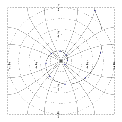
Figure 1: Flows $\phi_{0},\phi_{1}$ and solution of (4.1) obtained with $\Phi$ of fourth order.

4.2 Oscillatory reaction–diffusion system

In this example, we study the behavior of the methods of a reaction–diffusion system, as the ones shown in [17]. Since this system is an irreversible problem, symplectic methods with negative steps can not be used. We consider the system

$$\begin{split}\partial_{t}v=&\,\Delta v+(1-r^{2})v-(\omega_{0}-\omega_{1}r^{2})v,\\ \partial_{t}w=&\,\Delta w+(\omega_{0}-\omega_{1}r^{2})v+(1-r^{2})w,\end{split}$$ (4.2)

where $r^{2}=v^{2}+w^{2}$. If $u=v+iw$, equation (4.2) reads as follows:

$$\partial_{t}u=\Delta u+(1-|u|^{2})u+\mathrm{i}(\omega_{0}-\omega_{1}|u|^{2})u.$$

The right hand member can be written as $A_{0}u+A_{1}(u)$, where $A_{0}u=\Delta u$ and

$$A_{1}(u)=(1-|u|^{2})u+\mathrm{i}(\omega_{0}-\omega_{1}|u|^{2})u.$$

The flow $\phi_{1}$ is given by

$$\phi_{1}(h,u)=u\mathrm{e}^{h}(1+(\mathrm{e}^{2h}-1)|u|^{2})^{-1/2}\mathrm{e}^{\mathrm{i}(\omega_{0}h-\omega_{1}/2\ln(1+(\mathrm{e}^{2h}-1)|u|^{2}))}.$$

We will restrict our discussion to $L$–periodic solutions, flow $\phi_{0}$ can be computed approximately by using discrete Fourier transform (DFT). Let $\eta$ be an odd integer, $\eta=2l+1$ with $l\in\mathbb{N}$, consider

$$(I_{\eta}u)(x)=\sum\limits_{\nu=-{l}}^{{l}}\hat{U}_{\nu}\mathrm{e}^{\mathrm{i}a\nu x},$$

where $a=2\pi/L$ and $\hat{U}_{\nu}$ is the DFT coefficient given by

$$\hat{U}_{\nu}=\frac{1}{\eta}\sum_{r=0}^{\eta-1}U_{r}\mathrm{e}^{-\mathrm{i}2\pi r\nu/\eta}=\frac{1}{\eta}\sum_{r=0}^{\eta-1}u(Lr/\eta)\mathrm{e}^{-\mathrm{i}2\pi r\nu/\eta}.$$

Since $\mathrm{e}^{-\mathrm{i}2\pi r\nu/\eta}=\mathrm{e}^{-\mathrm{i}2\pi r(\nu\pm\eta)/\eta}$, it holds that $\hat{U}_{\nu}=\hat{U}_{\nu\pm\eta}$. From lemma 2.2. in [23], for $u\in\mathrm{H}^{\sigma}(\mathbb{T})$ with $\sigma>1/2$ we have that

$$\|u-I_{\eta}u\|_{L^{2}(\mathbb{T})}\leq C_{L,\sigma}\eta^{-\sigma}\|u\|_{\mathrm{H}^{\sigma}(\mathbb{T})}.$$

Thus we can derive the following proposition.

Proposition 4.1.

Let $\psi_{0}(h)=\phi_{0}(h)I_{\eta}$, then for $u\in\mathrm{H}^{\sigma}(\mathbb{T})$ with $\sigma>1/2$ it holds that

$$\|\psi_{0}(h)u-\phi_{0}(h)u\|_{L^{2}(\mathbb{T})}\leq C_{L,\sigma}\eta^{-\sigma}\|u\|_{\mathrm{H}^{\sigma}(\mathbb{T})}.$$

From the definition of $\psi_{0}(h)$ and using that $\hat{U}_{\nu}=\hat{U}_{\nu\pm\eta}$, we get

$$(\psi_{0}(h)u)(Lr/\eta)= \,\sum_{\nu=-l}^{l}\hat{U}_{\nu}\mathrm{e}^{-a^{2}\nu^{2}t}\mathrm{e}^{\mathrm{i}2\pi r\nu/\eta}=\sum_{\nu=l+1}^{\eta-1}\hat{U}_{\nu}\mathrm{e}^{-a^{2}(\eta-\nu)^{2}t}\mathrm{e}^{\mathrm{i}2\pi r\nu/\eta}$$

$$\,+\sum_{\nu=0}^{l}\hat{U}_{\nu}\mathrm{e}^{-a^{2}\nu^{2}t}\mathrm{e}^{\mathrm{i}2\pi r\nu/\eta}=\sum_{\nu=0}^{\eta-1}\hat{U}_{\nu}\mathrm{e}^{-a^{2}\lambda_{\nu}t}\mathrm{e}^{\mathrm{i}2\pi r\nu/\eta},$$

where $\lambda_{\nu}=\eta^{2}g(\nu/\eta)$ for $0\leq\nu\leq\eta-1$ and $g(\xi)=\xi^{2}-2(\xi-1/2)_{+}$.

In [17] the stability of the planar waves

$$v(x,t)= \,r^{*}\cos(\theta_{0}\pm ax+(\omega_{0}-\omega_{1}r^{*2})t),$$

$$w(x,t)= \,r^{*}\sin(\theta_{0}\pm ax+(\omega_{0}-\omega_{1}r^{*2})t),$$

is proven, if $L>2\pi(3+2\omega_{1}^{2})^{1/2}$, where $r^{*}=L^{-1}(L^{2}-4\pi^{2})^{1/2}$ and $\theta_{0}$ is an arbitrary constant (see also [22]). Taking $L=4\pi$, $\omega_{0}=1$, $\omega_{1}=1/2$ and $u_{0}=r^{*}\mathrm{e}^{iax}$, we compare methods given by (1.7b) of order $q=4,6,8$ with $\eta=63$. A similar analysis to that in remark 3.11 for the quasicontraction semi-group generated by $\Delta$ shows that the hypothesis of corollary 3.12 are satisfied. The fourth order method used is the same as the previous example, for the sixth order method we take $s=3$, $\gamma_{1}=1/48$, $\gamma_{2}=-8/15$ and $\gamma_{3}=81/80$, for the eighth order method we take $s=4$, $\gamma_{1}=-1/720$, $\gamma_{2}=8/45$, $\gamma_{3}=-729/560$ and $\gamma_{4}=512/315$. In figure 2 global errors for $T=10$ are shown. We note that the slopes coincide with the expected order up to the point where the rounding error dominates the total error.

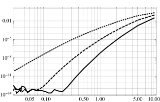
Figure 2: Global Error of $\Phi$ vs. $h$ for $q=4,6,8$

In order to show the stability of the planar waves, we consider the initial data $\tilde{u}_{0}(x)=0.8u_{0}(x)+0.1+2.5\mathrm{e}^{\mathrm{i}2ax}-0.8\mathrm{i}\mathrm{e}^{\mathrm{i}3ax}$. In figure 3 we can see the evolution of the fourth order method $\Phi(t,\tilde{u}_{0})$ for $t\in[0,50]$, calculated with $\eta=63$ and $h=0.1$ and $\phi(t,u_{0})$ is showed in dashed line.

Figure 3: $\mathrm{Re}(\Phi(t,\tilde{u}_{0}))$ for $t=0$ (left) and $t=50$ (right)

4.3 Regularized Schrödinger–Poisson equation

In this example, we study the $2\pi$–periodic solutions of the regularized Schrödinger–Poisson equation

$$\begin{cases}\partial_{t}u=\mathrm{i}\partial_{x}^{2}u-(-\partial_{x}^{2})^{\beta}u+\mathrm{i}|u|^{2}u+\mathrm{i}(G\ast|u|^{2})u,\\ u(0)=u_{0},\end{cases}$$ (4.3)

where $0<\beta<1$ and $G$ is a real kernel. Similar equations are considered in [1], [2] and [3], on bounded domains of $\mathbb{R}^{n}$ as well as on compact manifolds. In order to apply the methods given by (1.7b), we consider the flow $\phi_{0}$ generated by the linear operator $L=\mathrm{i}\partial_{x}^{2}-(-\partial_{x}^{2})^{\beta}$, and the flow $\phi_{1}(h,u)=\exp(\mathrm{i}h(|u|^{2}+G\ast|u|^{2}))u$ associated to $\partial_{t}u=\mathrm{i}(|u|^{2}+G\ast|u|^{2})u$. If $\rho=|u|^{2}$ and $\rho(x,t)=\sum_{\nu\in\mathbb{Z}}\hat{\rho}_{\nu}(t)\mathrm{e}^{\mathrm{i}\nu x}$, we have

$$(G\ast|u|^{2})(x,t)=\sum_{\nu\in\mathbb{Z}}\hat{G}_{\nu}\hat{\rho}_{\nu}(t)\mathrm{e}^{\mathrm{i}\nu x}$$

Both $\phi_{0}$, $\phi_{1}$ can be numerically solved using discrete Fourier transform as in the example above. Using FFT, the computational cost of each evaluation is $O(\eta\log\eta)$, where $\eta$ is the number of point in the spatial discretisation.

In order to analyse the performance of the integrators proposed, we consider the exact solutions $u(x,t)=r(t)\mathrm{e}^{\mathrm{i}(\nu_{0}x+\theta(t))}$, with $r(t)=r_{0}\mathrm{e}^{-|\nu_{0}|^{2\beta}t}$ and

$$\theta(t)=-\nu_{0}^{2}\,t+\frac{1}{2}(1+\hat{G}_{0})r_{0}^{2}|\nu_{0}|^{-2\beta}\left(1-\mathrm{e}^{-2|\nu_{0}|^{2\beta}t}\right)+\theta_{0}.$$

Note that $u(.,t)$ has only one oscillation mode, and taking $\nu_{0}$ as the momentum of the wave as it is usual, we can say that $u$ is a monokinetic wave. As an example, we consider the Poisson kernel given by

$$G(x)=\frac{\sinh(\lambda)}{\cosh(\lambda)-\cos(x)},$$

then $\hat{G}_{\nu}=\mathrm{e}^{-\lambda|\nu|}$. In figure 4, absolute global errors and relative global errors defined by

$$\mathcal{E}_{\mathrm{abs}}=\max_{0\leq n\leq[T/h]}\|u_{n}-U_{n}\|_{L^{2}},\quad\mathcal{E}_{\mathrm{rel}}=\max_{0\leq n\leq[T/h]}\frac{\|u_{n}-U_{n}\|_{L^{2}}}{\|u_{n}\|_{L^{2}}},$$

are shown, with $\beta=1/4$, $T=4$, $\lambda=1$, initial condition $u_{0}=\mathrm{e}^{\mathrm{i}4x}$ and methods varying from fourth to fourteenth order. The number of points in the spatial discretisation is $\eta=31$ and the temporal steps $h$ ranging from $0.01$ to $2$. Like in the example above the slopes coincide with the expected order up to the point where the rounding error dominates the total error.

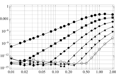
Figure 4: Global error vs. $h$ for $q=4,6,\ldots,14$, absolute error (left) and relative error (right)

For $\nu_{0}=0$, it holds $u(x,t)=r_{0}\mathrm{e}^{\mathrm{i}2|r_{0}|^{2}t+\mathrm{i}\theta_{0}}$ which are time periodic solutions. Multiplying (4.3) by $\bar{u}$ and integrating by parts, we get

$$\frac{d}{dt}\|u\|_{L^{2}}^{2}=-2\|(-\partial_{x}^{2})^{\beta/2}u\|_{L^{2}}^{2}=-2\mathop{\sum_{\nu\in\mathbb{Z}}}_{\nu\neq 0}|\nu|^{2\beta}|\hat{u}_{\nu}|^{2}\leq-2\|Pu\|_{L^{2}}^{2},$$

where $Pu=\sum_{\nu\neq 0}\hat{u}_{\nu}\mathrm{e}^{\mathrm{i}\nu x}$ and therefore the monokinetic solution with $\nu_{0}=0$ is the only time periodic solution.

It is easy to see that the flow $\phi$ of equation (4.3) preserves parity, then for any odd initial data $u_{0}$, $u(t)$ is an odd function and $u(t)=Pu(t)$ for $t>0$. Therefore, it holds $d\|u\|_{L^{2}}^{2}/dt\leq-2\|u\|_{L^{2}}^{2}$ and $\|u\|_{L^{2}}\leq\mathrm{e}^{-t}\|u_{0}\|_{L^{2}}$. We will test the numerical methods by verifying these properties. Consider the odd initial data $u_{0}(x)=\mathrm{e}^{\cos(2x)+\mathrm{i}\pi/6}\sin(5x)$, in figure 5 we show the numerical solution obtained with the eighth symmetric integrator with $\eta=255$ and $h=0.1$. Since the higher the frequencies are, the stronger is the damping, $u$ asymptotically behaves like $a\mathrm{e}^{-t-it}\sin(x)$.

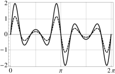
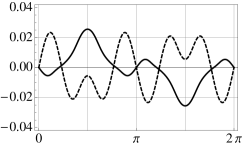
Figure 5: $\mathrm{Re}(\Phi(t,u_{0}))$ and $\mathrm{Im}(\Phi(t,u_{0}))$ for $t=0$ (left), $t=2$ (center) and $t=10$ (right)

In figure 6(a), it is shown the evolution of $\|u(.,t)\|_{L^{2}}/\|u_{0}\|_{L^{2}}$ in continuous line, the function $\mathrm{e}^{-t}$ in dotted line and the asymptotic behaviour in dashed line.

(a) Odd solution

(b) Even solution

Figure 6: Evolution of $\|u\|_{L^{2}}/\|u_{0}\|_{L^{2}}$ vs. time

We also consider a numerical computation with $u_{0}(x)=\mathrm{e}^{\cos(2x)+\mathrm{i}\pi/6}(1-1.75\cos^{2}(5x))$ an even initial data. Using the same integrator as in the odd case, we see that the solution converges to the periodic solution $u(x,t)\sim a\mathrm{e}^{i2|a|^{2}t}$ as it is seen in figure 7. In figure 6(b) it can be observed the fast stabilization of the norm. This suggests that the periodic solutions are limit cycles of the dynamic given by the equation (4.3).

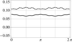
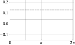
Figure 7: $\mathrm{Re}(\Phi(t,u_{0}))$ and $\mathrm{Im}(\Phi(t,u_{0}))$ for $t=0$ (left), $t=2$ (center) and $t=10$ (right)

References

- [1] L. Aloui. Smoothing effect for regularized Schrödinger equation on bounded domains. Asymptot. Anal., 59(3-4):179–193, 2008.
- [2] L. Aloui. Smoothing effect for regularized Schrödinger equation on compact manifolds. Collect. Math., 59(1):53–62, 2008.
- [3] L. Aloui, M. Khenissi, and G. Vodev. Smoothing effect for the regularized Schrödinger equation with non-controlled orbits. Comm. Partial Differential Equations, 38(2):265–275, 2013.
- [4] I. Aranson and L. Kramer. The world of the complex Ginzburg-Landau equation. Rev. Modern Phys., 74(1):99–143, 2002.
- [5] C. Besse, B. Bidégaray, and S. Descombes. Order estimates in time of splitting methods for the nonlinear Schrödinger equation. SIAM J. Numer. Anal., 40(1):26–40 (electronic), 2002.
- [6] J. P. Borgna, M. De Leo, D. Rial, and C. S. de la Vega. General splitting methods for abstract semilinear evolution equations. Commun. Math. Sci., 13(1):83–101, 2015.
- [7] F. Castella, P. Chartier, S. Descombes, and G. Vilmart. Splitting methods with complex times for parabolic equations. BIT, 49(3):487–508, 2009.
- [8] T. Cazenave. Semilinear Schrödinger equations, volume 10 of Courant Lecture Notes in Mathematics. New York University Courant Institute of Mathematical Sciences, New York, 2003.
- [9] S. Chin. Multi-product splitting and Runge-Kutta-Nyström integrators. Celestial Mech. Dynam. Astronom., 106(4):391–406, 2010.
- [10] K. Dekker and J. G. Verwer. Stability of Runge-Kutta methods for stiff nonlinear differential equations, volume 2 of CWI Monographs. North-Holland Publishing Co., Amsterdam, 1984.
- [11] S. Descombes and M. Thalhammer. An exact local error representation of exponential operator splitting methods for evolutionary problems and applications to linear Schrödinger equations in the semi-classical regime. BIT, 50(4):729–749, 2010.
- [12] Stéphane Descombes and Mechthild Thalhammer. The Lie-Trotter splitting for nonlinear evolutionary problems with critical parameters: a compact local error representation and application to nonlinear Schrödinger equations in the semiclassical regime. IMA J. Numer. Anal., 33(2):722–745, 2013.
- [13] L. Gauckler. Convergence of a split-step Hermite method for the Gross-Pitaevskii equation. IMA J. Numer. Anal., 31(2):396–415, 2011.
- [14] D. Goldman and T. J. Kaper. th-order operator splitting schemes and nonreversible systems. SIAM J. Numer. Anal., 33(1):349–367, 1996.
- [15] E. Hairer, S. P. Nørsett, and G. Wanner. Solving ordinary differential equations. I, volume 8 of Springer Series in Computational Mathematics. Springer-Verlag, Berlin, second edition, 1993. Nonstiff problems.
- [16] E. Hansen and A. Ostermann. High order splitting methods for analytic semigroups exist. BIT, 49(3):527–542, 2009.
- [17] N. Kopell and L. N. Howard. Plane wave solutions to reaction-diffusion equations. Studies in Appl. Mat., 52:291–328, 1973.
- [18] C. Lubich. On splitting methods for Schrödinger-Poisson and cubic nonlinear Schrödinger equations. Math. Comp., 77(264):2141–2153, 2008.
- [19] F. Neri. Lie algebras and canonical integration. Department of Physics report, University of Maryland, 1987.
- [20] Michael Reed and Barry Simon. Methods of modern mathematical physics. II. Fourier analysis, self-adjointness. Academic Press [Harcourt Brace Jovanovich, Publishers], New York-London, 1975.
- [21] R. D. Ruth. A canonical integration technique. IEEE Transactions on Nuclear Science, NS 30(4):2669–2671, 1983.
- [22] J. A. Sherratt. Periodic travelling wave selection by Dirichlet boundary conditions in oscillatory reaction-diffusion systems. SIAM J. Appl. Math., 63(5):1520–1538 (electronic), 2003.
- [23] E. Tadmor. The exponential accuracy of Fourier and Chebyshev differencing methods. SIAM J. Numer. Anal., 23(1):1–10, 1986.
- [24] H. Yoshida. Construction of higher order symplectic integrators. Phys. Lett. A, 150:262–268, 1990.