Fitting density models to observational data

We consider the general problem of fitting a parametric density model to discrete observations, taken to follow a non-homogeneous Poisson point process. This class of models is very common, and can be used to describe many astrophysical processes, including the distribution of protostars in molecular clouds. We give the expression for the likelihood of a given spatial density distribution of protostars and apply it to infer the most probable dependence of the protostellar surface density on the gas surface density. Finally, we apply this general technique to model the distribution of protostars in the Orion molecular cloud and robustly derive the local star formation scaling (Schmidt) law for a molecular cloud. We find that in this cloud the protostellar surface density, $\Sigma_{\mathrm{YSO}}$, is directly proportional to the square gas column density, here expressed as infrared extinction in the $K$-band, $A_{K}$: more precisely, $\Sigma_{\mathrm{YSO}}=($1.65\pm 0.19$)\,(A_{K}/$\mathrm{m}\mathrm{a}\mathrm{g}$)^{$2.03\pm 0.15$}\,$\mathrm{s}\mathrm{t}\mathrm{a}\mathrm{r}\mathrm{s}\,\mathrm{p}\mathrm{c}^{-2}$$.

1 Introduction

In this paper we address a general statistical problem: the fit of density models to discrete data. Consider a non-negative function $\rho(x|\theta)$, where $x\in\mathbb{R}^{d}$ is a point of a Euclidean space of dimension $d$ (in typical situations $d=1$, $2$, or $3$), and $\theta$ is a vector of model parameters. Suppose then that we observe a realization of a non-homogeneous Poisson point process with density $\rho(x|\theta)$: that is, suppose that we observe a random set of points $x_{n}\in\mathbb{R}^{d}$ distributed such that the number of points $N_{A,B}$ in two disjoint sets $A$ and $B$ of $\mathbb{R}^{d}$ are independent, and both $N_{A}$ and $N_{B}$ follow a Poisson distribution $P(N)=\mathrm{e}^{-\mu}\mu^{N}/N!$ with means

$$\mu_{A} {}=\int_{A}\rho(x|\theta)\,\mathrm{d}^{d}x\;, \mu_{B} {}=\int_{B}\rho(x|\theta)\,\mathrm{d}^{d}x\;.$$ (1)

We seek a way to infer the parameters $\theta$ from the points $\{x_{n}\}$.

The framework just introduced can be used to describe many different situations. For example, we could use it to model the stellar distribution in globular clusters, using the King model for the stellar positions; or we could use it to model the number counts of galaxies. Sarazin (1980) considered the same framework for fitting the distribution of galaxies in galaxy clusters. In this paper we use it to investigate the local Schmidt law of star formation in molecular clouds. In all cases we would be interested in inferring the relevant parameters of the density models used: center, richness, and concentration parameter for the King model; normalization, slope, and completeness limit for the number counts. In general, the relevant parameters $\theta$ can be constrained using a statistical frequentist approach, or a Bayesian approach. In both cases, we will need to evaluate the likelihood function, i.e. the conditional probability to observe a given set of data points $\{x_{n}\}$ given the value of the parameters $\theta$.

2 The log-likelihood

Suppose that we observe a set of $N$ points $\{x_{n}\}$ that we know are a realization of a random Poisson point process with a given density $\rho_{1}(x|\theta)$, which we assume to be normalized to unity:

$$\int\rho_{1}(x|\theta)\,\mathrm{d}^{d}x=1\;,$$ (2)

Since this function, from a statistical point of view, is a probability density, we can immediately write the likelihood of the configuration $\{x_{n}\}$ given the parameters $\theta$ as (Sarazin 1980)

$$\mathcal{L}\bigl{(}\{x_{n}\}|\theta\bigr{)}=\prod_{n=1}^{N}\rho_{1}(x_{n})\;.$$ (3)

More generally, if we deal with a spatial density $\rho(x|\theta)$ that is not normalized to unity, we can always consider the function

$$\rho_{1}(x|\theta) {}=\rho(x|\theta)/\mu\;, \mu {}\equiv\int\rho(x|\theta)\,\mathrm{d}^{d}x\;,$$ (4)

which by construction is normalized, and apply the likelihood (3) to $\rho_{1}$. However, this procedure prevents us from inferring any information on the normalizing constant $\mu$; additionally, it has the drawback of forcing us to deal with normalized densities, which in many contexts is not a natural choice.

To clarify these points, consider a simple model of star formation in nearby molecular clouds, where we postulate that

$$\Sigma_{\mathrm{YSO}}=\kappa\Sigma^{\beta}_{\mathrm{gas}}$$ (5)

where $\Sigma_{\mathrm{YSO}}$ is the surface density of protostars (stars pc^-2) in a molecular cloud and $\Sigma_{\mathrm{gas}}$ is the mass surface density ($\mathrm{M}_{$\odot$}\,\mathrm{p}\mathrm{c}^{-2}$) of the molecular gas. This relation is similar to the version of the well-known Schmidt Law (Schmidt 1959) introduced by Kennicutt (1998) which relates the globally averaged surface densities of the star formation rate ($\Sigma_{\mathrm{SFR}}$) and the gas ($\Sigma_{\mathrm{gas}}$) in galaxies in a power-law fashion. Suppose that we know the locations $\{x_{n}\}$ of $N$ protostars and the gas column density $\Sigma_{\mathrm{gas}}(x)$ in a region of the sky, and that we intend to infer the parameters $\kappa$ and $\beta$. In this case the likelihood discussed above does not provide any information on $\kappa$, and this is unfortunate since this parameter is directly linked to a critical piece of information, the star formation rate of the molecular cloud.

In order to solve this problem, we note that the probability density to observe $N$ points $\{x_{n}\}$ from $\rho(x|\theta)$ can be factorized as the probability to observe $N$ points (a Poisson distribution with mean $\mu$), and the probability that these $N$ points be located at the positions $\{x_{n}\}$ (as provided by Eq. (3)):

$$\mathcal{L}\bigl{(}[x_{n}]|\theta\bigr{)}=\mathrm{e}^{-\mu}\frac{\mu^{N}}{N!}\prod_{n=1}^{N}\rho_{1}\bigl{(}x_{n}|\theta\bigr{)}=\frac{1}{N!}\mathrm{e}^{-\int\rho(x)\,\mathrm{d}^{d}x}\prod_{n=1}^{N}\rho\bigl{(}x_{n}|\theta\bigr{)}\;.$$ (6)

In this expression the data points $[x_{n}]$ are taken to be ordered; if instead we consider the unordered set $\{x_{n}\}$, we just have to multiply this result by the number of permutations of $N$ elements, i.e. $N!$. With this choice, the log-likelihood takes the simple form

$$\ln\mathcal{L}\bigl{(}\{x_{n}\}|\theta\bigr{)}=\sum_{n=1}^{N}\ln\rho(x_{n}|\theta)-\int\rho(x|\theta)\,\mathrm{d}^{d}x\;.$$ (7)

3 Parameters inference

Using Bayes’ theorem

$$P\bigl{(}\theta|\{x_{n}\}\bigr{)}=\frac{\mathcal{L}\bigl{(}\{x_{n}\}|\theta\bigr{)}p(\theta)}{\int\mathcal{L}\bigl{(}\{x_{n}\}|\theta^{\prime}\bigr{)}p(\theta^{\prime})\,\mathrm{d}\theta^{\prime}}\;,$$ (8)

we can infer the posterior probability distribution of the parameters, $P\bigl{(}\theta|\{x_{n}\}\bigr{)}$ given the prior distribution $p(\theta)$. In our specific case, if we write $\rho(x|\theta)=\mu\rho_{1}(x|\theta)$, then the likelihood factorizes into the product of a term that depends only on $\mu$ and a term that depends on the other density parameters $\theta$. As a result, if the prior $p(\mu,\theta)=p(\mu)p(\theta)$ also factorizes, then the posterior distribution factorizes and $\mu$ is independent of $\theta$ (which implies that the two are also uncorrelated). In particular, if we use the uninformative improper prior $p(\mu)=1/\mu$ for $\mu>0$, we find that the posterior for $\mu$ is a simple Gamma distribution

$$P(\mu|\{x_{n}\})=\frac{\mathrm{e}^{-\mu}\mu^{N-1}}{\Gamma(N)}\;.$$ (9)

Below, as often the case in astronomy, we will deal with an unnormalized density $\rho$, and therefore we do not expect the various parameters $\theta$ to be independent.

4 Frequentist description

Alternatively, we can use to (log-)likelihood to obtain a maximum-likelihood point estimate of the parameters $\theta$ (Fisher 1922), i.e. find $\hat{\theta}=\mathop{\mathrm{arg\ max}}_{\theta}\ln\mathcal{L}$.

Bounds on the errors on the parameters can be evaluated from the Fisher information matrix (see, e.g., Feigelson & Babu 2012), that we recall is defined as

$$I_{ij}=\operatorname{E}\left[\frac{\partial\ln\mathcal{L}}{\partial\theta_{i}}\frac{\partial\ln\mathcal{L}}{\partial\theta_{j}}\right]=-\operatorname{E}\left[\frac{\partial^{2}\ln\mathcal{L}}{\partial\theta_{i}\,\partial\theta_{j}}\right]\;,$$ (10)

where the symbol $\operatorname{E}$ denotes the operation of ensemble average. The Fisher information matrix is related to the minimum covariance matrix that can be attained by an unbiased estimator, as provided by the Cramér-Rao bound:

$$\operatorname{Cov}(\hat{\theta})\geq I^{-1}\;.$$ (11)

Since the maximum-likelihood estimator is asymptotically efficient (i.e. it attains the Cramér-Rao bound when the sample size tends to infinity) and the resulting errors on $\hat{\theta}$ tend to a multivariate Gaussian distribution, it is interesting to obtain an analytic result for the information matrix. In Appendix A.2 we show that

$$I_{ij} {}=\int\frac{1}{\rho(x|\theta)}\frac{\partial\rho(x|\theta)}{\partial\theta_{i}}\frac{\partial\rho(x|\theta)}{\partial\theta_{j}}\,\mathrm{d}^{d}x$$

$${}=\int\rho(x|\theta)\frac{\partial\ln\rho(x|\theta)}{\partial\theta_{i}}\frac{\partial\ln\rho(x|\theta)}{\partial\theta_{j}}\,\mathrm{d}^{d}x\;.$$ (12)

Finally, we can evaluate the goodness of the fit obtained by comparing the maximum likelihood value with what we are expected to obtain. The expected (average) likelihood can be estimated analytically by performing an ensemble average over the points $\{x_{n}\}$. As show in Appendix A.2, the average value of the log-likelihood calculated at the true value of the parameters is

$$\operatorname{E}[\ln\mathcal{L}](\theta)=\int\rho(x|\theta)\bigl{[}\ln\rho(x|\theta)-1\bigr{]}\,\mathrm{d}^{d}x\;.$$ (13)

For our purposes it is more relevant to obtain the expectation value of the likelihood at its maximum value $\hat{\theta}$: this value can then be compared with the observed maximum of the log-likelihood to provide a goodness-of-fit proxy. The result obtained is

$$\operatorname{E}[\ln\mathcal{L}](\hat{\theta})=\operatorname{E}[\ln\mathcal{L}](\theta)+\frac{J}{2}\;,$$ (14)

where $J$ is the number of the free parameters in the density, i.e. the dimensionality of the space of $\theta$.

Finally, the variance of the log-likelihood is provided by

$$\operatorname{Var}[\ln\mathcal{L}](\hat{\theta})=\int\rho(x|\theta)\ln^{2}\rho(x|\theta)\,\mathrm{d}^{d}x\;.$$ (15)

This expression, together with Eq. (14) is useful to define acceptance boundaries for the likelihood value and therefore for model test.

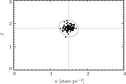
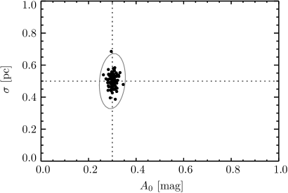
Figure 1: Maximum likelihood best-fit parameters for a set of 100 simulations. The dotted lines show the true, original values used: $\kappa=$1.5\text{\,}\mathrm{s}\mathrm{t}\mathrm{a}\mathrm{r}\,\mathrm{p}\mathrm{c}^{-2}$$, $\beta=1.8$, $A_{0}=$0.3\text{\,}\mathrm{m}\mathrm{a}\mathrm{g}$$, and $\sigma=$0.5\text{\,}\mathrm{p}\mathrm{c}$$. Note how the points, representing the individual best-fits, cluster around the true values. The ellipses, showing the expected 3-$\sigma$ errors as deduced from the Fischer information matrix, are in excellent agreement with the observed distribution of points.

5 Application: deriving the local Schmidt scaling law for a giant molecular cloud

In this section we apply the framework developed above to one relevant astrophysical problem, determining the local star formation scaling law for a nearby Giant Molecular Cloud, which in its simplest version can be written as in Eq. (5).

In nearby molecular clouds $\Sigma_{\mathrm{YSO}}$ is a directly measured quantity and can be related to $\Sigma_{\mathrm{SFR}}$ via $\Sigma_{\mathrm{SFR}}=\Sigma_{\mathrm{YSO}}\times\langle m\rangle/\tau$, where $\langle m\rangle$ is the mean mass of a protostar and $\tau$ the age of the protostellar (class I) population in the cloud. We note here that we are interested in the local star formation scaling law within a GMC and this is physically different from the Kennicutt-Schmidt law which relates global quantities averaged over entire galaxies (e.g., Kennicutt 1998) or subregions of galaxies (e.g., Bigiel et al. 2008) which in either case do not resolve the individual molecular clouds. Indeed, the indexes ($\beta$) of the local and global relations are not necessarily physically related, nor expected to be the same, when comparing individual molecular clouds and normal galaxies (e.g., Calzetti et al. 2012).

Since we use infrared extinction measurements to trace the gas column density in the clouds we write Eq. (5) as $\Sigma_{\mathrm{YSO}}\propto A_{K}^{\beta}$ and note that $\Sigma_{\mathrm{gas}}\propto A_{K}$ for a constant gas-to-dust ratio. Additionally we allow for the possibility of a star-formation threshold, i.e., a lower limit of the surface density for gas, or equivalently dust, below which no star formation takes place and no protostars are produced in situ (e.g., Lada et al. 2010, Heiderman et al. 2010). Finally, since it is physically reasonable to assume that star formation is not an instantaneous process, we allow for some diffusion of protostars from their birth sites. We model this diffusion process by smoothing the initial protostellar surface density, $\Sigma_{\mathrm{YSO}}^{(0)}$, by a Gaussian spatial kernel. In summary we have

$$\Sigma_{\mathrm{YSO}}(x|\kappa,\beta,A_{0},\sigma)=\int\frac{1}{2\pi\sigma^{2}}\mathrm{e}^{|x-x^{\prime}|^{2}/2\sigma^{2}}\Sigma_{\mathrm{YSO}}^{\mathrm{(0)}}(x^{\prime}|\kappa,\beta,A_{0})\,\mathrm{d}^{2}x^{\prime}\;,$$ (16)

where

$$\Sigma_{\mathrm{YSO}}^{\mathrm{(0)}}(x|\kappa,\beta,A_{0})=\kappa\operatorname{H}\bigl{(}A_{K}(x)-A_{0}\bigr{)}\left(\frac{A_{K}}{$1\text{\,}\mathrm{m}\mathrm{a}\mathrm{g}$}\right)^{\beta}(x)\;.$$ (17)

In this equation $\operatorname{H}$ is the Heaviside step function (defined to be zero for a negative argument and one for positive one). The constants involved are the normalization $\kappa$ (taken to be measured in units of $\mathrm{s}\mathrm{t}\mathrm{a}\mathrm{r}\,\mathrm{p}\mathrm{c}^{-2}\,\mathrm{m}\mathrm{a}\mathrm{g}^{-\beta}$, the star-formation threshold $A_{0}$ (in units of $K$-band extinction), the dimensionless exponent $\beta$, and the diffusion coefficient $\sigma$ (measured in pc).

The data at our disposal will be the extinction map of a molecular cloud, i.e. $A_{K}(x)$, and a catalog with the positions of protostars $\{x_{n}\}$. With these data we can fit the four parameters $\theta=\{\kappa,\beta,A_{0},\sigma\}$ using both the approaches described in Sects. 3 and 4.

5.1 Simulations

Before using the techniques described in this paper on real data, we validated them on simulated data. The simulations were carried out by taking the extinction map of the Orion molecular cloud from Lombardi et al. (2011), and by randomly generating protostars according to the law (16). Specifically, we fixed the parameters $\beta$, $A_{0}$, and $\sigma$ to test values, and we set $\kappa$ such that the expected number of protostars in the field was $300$. For each simulation, we then drew the number of protostars from a Poisson distribution with the appropriate average, and we distributed the initial positions of the stars in the field following the density $\Sigma_{\mathrm{YSO}}^{\mathrm{(0)}}$ of Eq. (17), i.e. without any diffusion represented by the $\sigma$ parameters. Finally, we changed the initial positions of the protostars by drawing random offsets from a two dimensional normal distribution with variance $\sigma^{2}$, and by moving each protostar position according to the drawn offsets.

We then tried to recover the “unknown” parameters using both a maximum likelihood approach and a Bayesian inference. The input data provided to the code were the positions of the protostars, as generated using the procedure described above, and the extinction map of the cloud. Figure 1 reports the results obtained in a typical set of simulation with true parameters $\kappa=$1.5\text{\,}\mathrm{s}\mathrm{t}\mathrm{a}\mathrm{r}\,\mathrm{p}\mathrm{c}^{-2}\,\mathrm{m}\mathrm{a}\mathrm{g}^{-\beta}$$, $\beta=1.8$, $A_{0}=$0.3\text{\,}\mathrm{m}\mathrm{a}\mathrm{g}$$, and $\sigma=$0.5\text{\,}\mathrm{p}\mathrm{c}$$. To produce the plots, we performed 100 independent simulations, drawing each time a different set of protostars, and we report in the plot the locations of the best-fit estimates obtained from the maximization of the likelihood. We also plot the expected 3-$\sigma$ error ellipse, as derived from the Fisher information matrix. As expected, and as shown by these plots (and analogous ones produced during our tests), the maximum likelihood estimate does not suffer any evident bias and is able to constrain all parameters in a very efficient way. Note that for the set of simulations shown in Fig. 1 we used on average $300$ protostars, a number comparable with the number of class I objects known in Orion A (see below). During the tests we also verified that the value of the likelihood function at its maximum was compatible with the expectations of Eqs. (14) and (15).

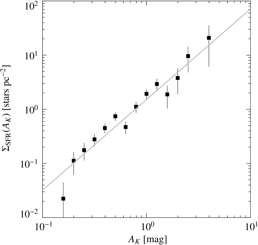
Figure 2: The differential distribution of $\Sigma_{\mathrm{SFR}}$ as a function of extinction on a simulation carried out with input parameters $\kappa=$1.5\text{\,}\mathrm{s}\mathrm{t}\mathrm{a}\mathrm{r}\,\mathrm{p}\mathrm{c}^{-2}\,\mathrm{m}\mathrm{a}\mathrm{g}^{-\beta}$$, $\beta=1.8$, $A_{0}=$0.3\text{\,}\mathrm{m}\mathrm{a}\mathrm{g}$$, and $\sigma=$0.5\text{\,}\mathrm{p}\mathrm{c}$$. The best-fit power law, shown as a line in this plot, is $\kappa=$1.23\pm 0.12\text{\,}\mathrm{s}\mathrm{t}\mathrm{a}\mathrm{r}\,\mathrm{p}\mathrm{c}^{-2}\,\mathrm{m}\mathrm{a}\mathrm{g}^{-\beta}$$ and $\beta=$2.71\pm 0.08$$.

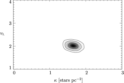
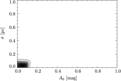
Figure 3: The posterior probability for the four density parameters obtained for the Orion A molecular cloud.

We also tested in a similar way the Bayesian approach. For these tests, we adopted both uniform and uninformative Jeffreys priors for the parameters, excluding for all of them negative values. In general, during our tests we found that original, true values of the parameters were always within the Bayesian $95\%$ credible intervals.

As a comparison, Fig. 2 shows the projected density of protostars as a function of the projected density of the dust. To make this figure, we considered increasing contour levels of extinction, and we estimated the density of protostars within two consecutive levels of extinction by computing the ratio between the number of protostars and the area enclosed within the two contours; errors were estimated from simple Poisson statistics. The figure also shows the best-fit power law obtained from these data, which is not in agreement with the original input: the measured parameters where $\kappa=$1.23\pm 0.12\text{\,}\mathrm{s}\mathrm{t}\mathrm{a}\mathrm{r}\,\mathrm{p}\mathrm{c}^{-2}\,\mathrm{m}\mathrm{a}\mathrm{g}^{-\beta}$$ and $\beta=$2.71\pm 0.08$$, compared with the original input parameters of $\kappa=$1.5\text{\,}\mathrm{s}\mathrm{t}\mathrm{a}\mathrm{r}\mathrm{s}\,\mathrm{p}\mathrm{c}^{-2}\,\mathrm{m}\mathrm{a}\mathrm{g}^{-\beta}$$ and $\beta=1.8$. This simple test shows that in presence of a threshold and/or of a diffusion of the protostars from their original loci of formation, the standard fit of the $\Sigma_{\mathrm{gas}}$–$\Sigma_{\mathrm{SFR}}$ plot leads to unreliable results. Note that the poor performance of the simple fit of histograms is a combination of several factors: the use of a simple least-squares minimization algorithm does not take into account the Poisson statistics of the bins (see Laurence & Chromy 2010); the lack of modeling of the threshold and of the diffusion; the lost of information when binning the data. A partial removal of these factors occasionally makes the algorithm less biased (but only marginally so); in some cases (particularly when adding the parameter $A_{0}$ to the fit) the bias was actually larger, presumably as a result of a poor minimization of the least square algorithm. In general, we find that the fitting algorithm based on binned data is very unstable, leading to large differences in the results depending on the particular configuration used (i.e., on the specific location of the protostars $\{x_{n}\}$ and on the particular choice of the bin sizes). Note instead that the use of a Poisson statistics with infinitesimal bins produces the same likelihood of Eq. (6) (see Appendix A.1), and therefore guarantees unbiased and robust results.

Additionally, we also checked the results of the Bayesian analysis when other observational effects were present in the data. Specifically, after generating the stars according to the local Schmidt law, we convolved the map with a Gaussian beam with $\mathit{FWHM}=$6\text{\,}\mathrm{a}\mathrm{r}\mathrm{c}\mathrm{m}\mathrm{i}\mathrm{n}$$ to simulate the effect of a unresolved structures due to finite resolution. Moreover, we added artificial noise that takes into account the proper error propagation in the extinction map (see Lombardi & Alves 2001). Simulations showed that the Bayesian technique can cope well with these effects, and the results obtained are largely unaffected.

In summary, the simulations completely validated the approach described in this paper. We therefore applied our method to the best studied star-forming molecular cloud, the Orion complex.

5.2 Application to Orion A

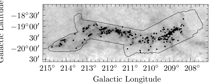
Figure 4: The extinction map of Orion A (taken from Lombardi et al. 2011), together with the location of the Class I protostars (from Megeath et al. 2012). The polygonal line shows the region where the protostar observations have been carried out.

In order to derive the local Schmidt scaling law in Orion-A, we used our 2MASS/Nicest extinction map (Lombardi et al. 2011). We preferred the Nicest (Lombardi 2009) algorithm over the Nicer (Lombardi & Alves 2001) one because the former produces maps that are less affected by systematic biases in the central regions of molecular clouds, where presumably most protostars are formed. Additionally, we used a catalog of protostars obtained from a survey carried out in the region with Spitzer Space Telescope (Megeath et al. 2012). From this catalog we selected only Class I sources (specifically, objects classified as “probable protostars”); moreover, we excluded 56 sources found by cross-correlation with a catalog of 624 foreground objects (identified as unreddened sources visible in front of the molecular cloud, see Alves & Bouy 2012). As a result, we were left with 329 objects enclosed within the polygonal area in Orion-A where the observations have been carried out (see Megeath et al. 2012 for details on the area selection).

We performed frequentist and a Bayesian analyses of these data using the techniques described in this paper. For the Bayesian analysis we fitted the model (16) with flat priors over all parameters (taken however to be positive) using the likelihood of Eq. (7). We explored the resulting posterior probability distribution with Markov Chain Monte Carlo, using a simple Metropolis-Hastings sampler. The resulting posterior probability, shown in Fig. 3, presents the following relevant results (all bounds are referred to a $95\%$ confidence level interval):

• The exponent $\beta$ is exquisitely close to the value $2$: the result obtained is indeed $\beta=2.03\pm 0.15$.

• We measure a star-formation coefficient $\kappa=$1.65\pm 0.19\text{\,}\mathrm{s}\mathrm{t}\mathrm{a}\mathrm{r}\,\mathrm{p}\mathrm{c}^{-2}\,\mathrm{m}\mathrm{a}\mathrm{g}^{-2}$$.

• The data show that there is no threshold for star formation: $A_{0}<$0.09\text{\,}\mathrm{m}\mathrm{a}\mathrm{g}$$.

• Class I protostars seem to have undergone no detectable diffusion from their original positions beyond the resolution of our extinction maps.

The frequentist analysis provides consistent results. Here we just mention the fact that the best-fit log-likelihood is $\ln\mathcal{L}(\hat{\theta})=-1156$; as a reference, the value predicted from Eq. (14) is $\operatorname{E}[\ln\mathcal{L}](\hat{\theta})=-1137$, with an expected tolerance computed from the square root of Eq. (15) of $\sim 52$. We deduce therefore that the model proposed is in agreement with the observations.

5.3 Discussion

Using the analysis described above we can now write the fundamental star formation scaling relation for the Orion A molecular cloud:

$$\Sigma_{\mathrm{YSO}}=($1.65\pm 0.19$)\left(\frac{A_{K}}{$\mathrm{m}\mathrm{a}\mathrm{g}$}\right)^{$2.03\pm 0.15$}\,$\mathrm{s}\mathrm{t}\mathrm{a}\mathrm{r}\,\mathrm{p}\mathrm{c}^{-2}$\;.$$ (18)

This result can be considered a complete description of the local Schmidt law characterizing this cloud because our analysis has enabled the derivation of robust values for both the power-law index, $\beta$, and the coefficient, $\kappa$, the constant of proportionality. While $\beta$ determines how $\Sigma_{\mathrm{YSO}}$ varies with column density of the cloud, $\kappa$ sets the overall scale or magnitude of the relation.

It is of interest to compare our results to those of a few recently published studies. Gutermuth et al. (2011) derived a value for $\beta$ of $1.8\pm 0.01$ for the Orion cloud from a least-squares fit to the $\Sigma_{\mathrm{YSO}}$–$\Sigma_{\mathrm{gas}}$ relation, using the nearest neighbor method to derive $\Sigma_{\mathrm{YSO}}$ for each star and infrared extinction measurements to derive the corresponding $\Sigma_{\mathrm{gas}}$. This result is in reasonable agreement with our findings, particularly given the large scatter in the Gutermuth et al. (2011) data. Steeper $\beta$s ($\sim 4$), however, have been derived for other clouds using different methodologies (Heiderman et al. 2010; Harvey et al. 2013). Whether this represents evidence for variations in $\beta$ between clouds is far from clear at this time. More robust statistics and application of a more consistent methodology to studies of other clouds would be needed to make a better comparison to our results for Orion and a better assessment of possible cloud-to-cloud variations in the star formation scaling law. We started already a follow-up analysis in this direction, and the results of the application of the statistical technique described in this paper to a set of clouds are presented in Lada et al. (2013), to which we refer the reader for a more the astrophysical conclusions of the analysis.

5.4 Concluding Remarks

In this paper we described the use of a likelihood analysis to derive a parametric density model that best describes the discrete spatial data. The likelihood can be used both in a frequentist and Bayesian analysis, and appears to be validated by its application to simulated data in which input parameters were accurately recovered. We applied the method to model the observed distribution of Class I protostars in the Orion A molecular cloud and derive the star formation scaling law for that cloud. Specifically we find: $\Sigma_{\mathrm{YSO}}=($1.65\pm 0.19$)\,(A_{K}/$\mathrm{m}\mathrm{a}\mathrm{g}$)^{$2.03\pm 0.15$}\,$\mathrm{s}\mathrm{t}\mathrm{a}\mathrm{r}\mathrm{s}\,\mathrm{p}\mathrm{c}^{-2}$$. Moreover, we found no evidence for an extinction threshold for star formation in the cloud and no evidence for any significant diffusion of the protostars from their birth sites.

Appendix A Analytical derivations

A.1 Alternative derivation of Eq. (7)

In this section we provide an alternative derivation of Eq. (7), that highlights the relationship between the likelihood and the fit of histograms. Suppose we that we know completely the density $\rho(x)\equiv\rho(x|\theta)$ responsible for a Poisson point process. One possibility to evaluate the probability to observe a given configuration $\{x_{n}\}$ of points is to make a partition of the domain of $\rho(x)$ into a small regions or bins of equal area $a$, chosen such that $a\ll 1/\rho(x)$ for any point $x\in\mathbb{R}^{d}$. In this way, since the average number of stars for each bin is much less then unity, then each bin will contain at most one point. In this limit, each bin will have with probability $P_{0}(x)=1-a\rho(x)$ no stars, and with probability $P_{1}(x)=a\rho(x)$ one star. The joint probability for the whole configuration will be therefore the product of the individual probabilities for the individual bins, i.e.

$$P\bigl{(}\{x_{n}\}|\theta\bigr{)}=\prod_{n=1}^{N}\bigl{[}a\rho(x_{n}|\theta)\big{]}\prod_{m}\bigl{[}1-a\rho(x_{m}|\theta)\bigr{]}\;,$$ (19)

where the first product runs over the $N$ bins with a single data point, and the second one over the other bins, i.e. all bins without any data point (we recall that since bins are taken to be small, no bin has more than a datapoint). This probability is proportional to $a^{N}$, and therefore as we take the limit $a\rightarrow 0$ it is interesting to consider $\mathcal{L}=P/a^{N}$: that operation corresponds to use a probability density. If we switch to logarithms, the first product over $n$ becomes a sum of $\ln\rho$ at the locations of the points, while the second product, in the limit of $a\rightarrow 0$, becomes an integral over the entire space (because the bins with points make a negligible contribution, see Fig. 5):

$$\ln\mathcal{L}\bigl{(}\{x_{n}\}|\theta\bigr{)}=\sum_{n=1}^{N}\ln\rho(x_{n}|\theta)-\int\rho(x|\theta)\,\mathrm{d}^{d}x\;.$$ (20)

A.2 Properties of the log-likelihood

In order to prove Eq. (13), we note that the average has to be carried out over all possible configurations of data points $\{x_{n}\}$, and therefore involves only the first term, i.e. the summation, of this equation; the integral is a constant term and the average is trivially itself. Let us call $\ell$ the first term of Eq. (13), and $\mu$ the second, so that $\ln\mathcal{L}=\ell+\mu$. By using the same reasoning of Eq. (6), we can write the average of $\ell$ by considering separately the probability to have exactly $N$ points in the field, which follows a Poisson probability, and the probability for the distribution of each of these points. In summary,

$$\operatorname{E}[\ell] {}=\sum_{N=0}^{\infty}\mathrm{e}^{-\mu}\frac{\mu^{N}}{N!}\int\mathrm{d}x_{1}\,\frac{\rho(x_{1})}{\mu}\cdots\int\mathrm{d}x_{N}\,\frac{\rho(x)}{\mu}\ell\;$$

$${}=\sum_{N=0}^{\infty}\frac{\mathrm{e}^{-\mu}}{N!}\int\mathrm{d}x_{1}\,\rho(x_{1})\cdots\int\mathrm{d}x_{N}\,\rho(x_{N})\sum_{n=1}^{N}\ln\rho(x_{n})$$

$${}=\sum_{N=0}^{\infty}\mathrm{e}^{-\mu}\frac{\mu^{N-1}}{N!}\sum_{n=1}^{N}\int\mathrm{d}x_{n}\,\rho(x_{n})\ln\rho(x_{n})$$

$${}=\sum_{N=1}^{\infty}\mathrm{e}^{-\mu}\frac{\mu^{N-1}}{(N-1)!}\int\mathrm{d}x\,\rho(x)\ln\rho(x)$$

$${}=\int\mathrm{d}x\,\rho(x)\ln\rho(x)\;.$$ (21)

Finally, putting back the term $\mu$ of $\ln\mathcal{L}$ we obtain the desired result of Eq. (13).

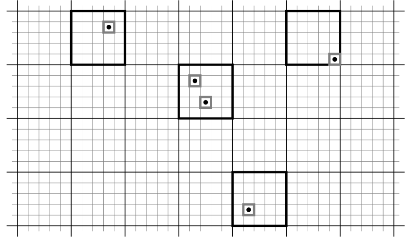
Figure 5: The derivation of the likelihood of Eq. (7). Note that when we reduce the grid size from the black grid to the grey one, each grid cell eventually contains at most one point. Note also how the total area of the grid cells with points becomes negligible when the grid size is small.

The variance of $\ln\mathcal{L}$ is identical to the variance of $\ell$, which can be evaluated from $\operatorname{E}[\ell^{2}]$. Following a calculation similar to Eq. (3) and using the independence of $x_{n}$ from $x_{m}$ for $n\neq m$ one obtains

$$\operatorname{E}[\ell^{2}]=\left[\int\rho(x)\ln\rho(x)\,\mathrm{d}^{d}x\right]^{2}+\int\rho(x)\ln^{2}\rho(x)\,\mathrm{d}^{d}x\;.$$ (22)

From this equation one immediately derives $\operatorname{Var}(\mathcal{L})=\operatorname{Var}(\ell)=\operatorname{E}(\ell^{2})-\operatorname{E}^{2}(\ell)$ as given in Eq. (15).

In a similar way one can derive Eq. (4). We start from the second equality of Eq. (10), and we note that the partial derivatives of $\ln\mathcal{L}$ can be written as

$$-\frac{\partial^{2}\ln\mathcal{L}}{\partial\theta_{i}\,\partial\theta_{j}}={} \sum_{n=1}^{N}\left[\frac{1}{\rho^{2}(x_{n})}\frac{\partial\rho(x_{n})}{\partial\theta_{i}}\frac{\partial\rho(x_{n})}{\partial\theta_{j}}-\frac{1}{\rho(x_{n})}\frac{\partial^{2}\rho(x_{n})}{\partial\theta_{i}\,\partial\theta_{j}}\right]$$

$${}-\int\frac{\partial^{2}\rho(x_{n})}{\partial\theta_{i}\,\partial\theta_{j}}\,\mathrm{d}^{d}x\;.$$ (23)

When taking the average over the point positions $\{x_{n}\}$ of this expression, the summation of the first line becomes an integral over $\rho(x)\,\mathrm{d}^{d}x$, and as a result the last term of the first line cancels with the integral of the second line. We are therefore left out with Eq. (4).

References

- Alves & Bouy (2012) Alves, J. & Bouy, H. 2012, A&A, 547, A97
- Bigiel et al. (2008) Bigiel, F., Leroy, A., Walter, F., et al. 2008, AJ, 136, 2846
- Calzetti et al. (2012) Calzetti, D., Liu, G., & Koda, J. 2012, ApJ, 752, 98
- Feigelson & Babu (2012) Feigelson, E. D. & Babu, G. J. 2012, Modern Statistical Methods for Astronomy (Cambridge University Press)
- Fisher (1922) Fisher, R. A. 1922, Royal Society of London Philosophical Transactions Series A, 222, 309
- Gutermuth et al. (2011) Gutermuth, R. A., Pipher, J. L., Megeath, S. T., et al. 2011, ApJ, 739, 84
- Harvey et al. (2013) Harvey, P. M., Fallscheer, C., Ginsburg, A., et al. 2013, ApJ, 764, 133
- Heiderman et al. (2010) Heiderman, A., Evans, II, N. J., Allen, L. E., Huard, T., & Heyer, M. 2010, ApJ, 723, 1019
- Kennicutt (1998) Kennicutt, Jr., R. C. 1998, ApJ, 498, 541
- Lada et al. (2013) Lada, C., Lombardi, M., Roman-Zuniga, C., Forbrich, J., & Alves, J. 2013, ApJ, in press (astro-ph/1309.7055)
- Lada et al. (2010) Lada, C. J., Lombardi, M., & Alves, J. F. 2010, ApJ, 724, 687
- Laurence & Chromy (2010) Laurence, T. A. & Chromy, B. A. 2010, Nature Methods, 7, 338
- Lombardi (2009) Lombardi, M. 2009, A&A, 493, 735
- Lombardi & Alves (2001) Lombardi, M. & Alves, J. 2001, A&A, 377, 1023
- Lombardi et al. (2011) Lombardi, M., Alves, J., & Lada, C. J. 2011, A&A, 535, A16
- Megeath et al. (2012) Megeath, S. T., Gutermuth, R., Muzerolle, J., et al. 2012, AJ, 144, 192
- Sarazin (1980) Sarazin, C. L. 1980, ApJ, 236, 75
- Schmidt (1959) Schmidt, M. 1959, ApJ, 129, 243