Quantum theory of multimode polariton condensation

Abstract

We develop a theory for the dynamics of the density matrix describing a multimode polariton condensate. In such a condensate several single-particle orbitals become highly occupied, due to stimulated scattering from reservoirs of high-energy excitons. A generic few-parameter model for the system leads to a Lindblad equation which includes saturable pumping, decay, and condensate interactions. We show how this theory can be used to obtain the population distributions, and the time-dependent first- and second-order coherence functions, in such a multimode condensate. As a specific application, we consider a polaritonic Josephson junction, formed from a double-well potential. We obtain the population distributions, emission line shapes, and widths (first-order coherence functions), and predict the dephasing time of the Josephson oscillations.

I Introduction

The strong coupling of quantum well excitons and microcavity photons gives rise to part-light and part-matter quasiparticles known as cavity polaritons.Hopfield (1958); Weisbuch et al. (1992) Polaritons inherit the bosonic nature of their constituents, allowing them to undergo Bose-Einstein condensation.Dang et al. (1998); Kasprzak et al. (2006); Love et al. (2008); Assmann et al. (2011) The condensation is characterized by the appearance of macroscopically occupied single-particle states in a pumped microcavity. It differs from Bose-Einstein condensation in atomic gases,Pitaevskii and Stringari (2003) because the polaritons have a very light effective mass, and can therefore condense at a much higher background temperature. Another key distinction between polariton condensates and their atomic counterparts is the fact that polaritons decay into external photons, typically in a few picoseconds. Thus, the polariton condensate is a nonequilibrium steady-state, maintained by a balance between the radiative decay and the external pumping. The external pumping generally creates a population of excitons or polaritons at high energy, and condensation occurs in lower energy states due to stimulated scattering from the high-energy reservoir.

One consequence of this nonequilibrium nature is that, whereas in equilibrium only the lowest energy single-particle state can be macroscopically occupied, for polaritons large occupations can build up in other orbitals. Furthermore, the condensation can occur in several orbitals simultaneously, enabling the study of interacting macroscopic quantum states. The presence of several highly occupied states of a trapping potential can be seen directly in the emission spectra,Tosi et al. (2012); Galbiati et al. (2012) and inferred from the presence of Josephson oscillations.Lagoudakis et al. (2010); Abbarchi et al. (2013) Such multimode condensation can also occur in spatially extended states, in particular in the Bloch states of oneLai et al. (2007) and twoMasumoto et al. (2012) dimensional lattices. The in-plane potentials that control these condensates can arise from growth induced disorder in the Bragg mirrors,Langbein et al. (1999); Love et al. (2008); Lagoudakis et al. (2010) metal-film patterning of the mirror surfaces,Lai et al. (2007); Masumoto et al. (2012) and interaction effects,Tosi et al. (2012) as well as from the use of non-planar structures such as micropillars and photonic molecules.Galbiati et al. (2012)

The theoretical modeling of these nonequilibrium quantum objects has been performed quite extensively within the mean-field approximation, using an augmented Gross-Pitaevskii descriptionWouters and Carusotto (2007); Keeling and Berloff (2008); Eastham (2008); Rodrigues et al. (2012) to treat the dynamics of the highly occupied orbitals, and to obtain the excitation spectra. Mean-field solutions of microscopic models using the nonequilibrium Green’s function formalismSzymańska et al. (2007) have also been developed. The LangevinTassone and Yamamoto (2000); Haug et al. (2012); Wouters and Savona (2009), Fokker-PlanckWhittaker and Eastham (2009); Schwendimann et al. (2010), and density matrixPorras and Tejedor (2003); Laussy et al. (2004); Verger et al. (2006); Schwendimann and Quattropani (2008); Savenko et al. (2011) frameworks have been used to derive the quantum statistics of the condensate, and hence the first- and second-order coherence functions of the optical emission. The density matrix approach allows the treatment of fluctuations in the condensate as well as the direct incorporation of incoherent phenomena such as the interaction with phonon baths.Laussy et al. (2004); Savenko et al. (2011) While mean field theories are already able to treat several highly occupied orbitals,Eastham (2008); Wouters (2008); Rodrigues et al. (2012) full quantum treatments of this regime have yet to be formulated.

The aim of this work is to develop a density matrix approach for multimode polariton condensation, in which several single-particle orbitals are driven by several reservoirs. It treats both quantum and nonequilibrium fluctuations, and allows photon statistics and emission spectra to be calculated. We first derive a Lindblad equation for two condensate modes (highly occupied orbitals) pumped by a single reservoir of higher energy particles, using a treatment similar to that of a two-mode laser,Singh and Zubairy (1980) and then extend the result to treat several reservoirs pumping several condensates. This gives a generic model for the quantum dynamics of a nonequilibrium polariton condensate, with the complexity of the reservoirs captured in a few known parameters. We show how the theory can be used to obtain the population distribution of the condensate orbitals, both numerically and analytically. We also show how it may be used to calculate both first-order and second-order coherence functions. The first-order coherence function, $\langle a_{1}^{\dagger}(\tau)a_{1}\rangle$, is the Fourier transform of the emission spectrum from one condensate orbital. We obtain it in three different ways: (i) direct numerical solution of the Lindblad form, (ii) making a continuum approximation to obtain a soluble partial differential equation, related to the Fokker-Planck equation,Kampen (2007); Whittaker and Eastham (2009) and (iii) a cruder static limit approximation, which neglects the dynamics of the populations, but is generally valid near threshold.Whittaker and Eastham (2009) Among higher order correlation functions we consider those of the form $\langle a_{1}^{\dagger}(\tau)a_{2}(\tau)a_{2}^{\dagger}a_{1}\rangle$, which quantify the dephasing of the intensity oscillations that correspond to the beating between the condensate modes. Such oscillations are a form of Josephson oscillations, which have been observed experimentally.Lagoudakis et al. (2010) We analyze their dephasing both numerically and in the static limit.

As a specific application of our theory, we study fluctuations in a polariton Josephson junction, formed in a double-well potential,Lagoudakis et al. (2010) using a tight-binding model in which each well is pumped by a corresponding reservoir. Diagonalizing the Hamiltonian leads to symmetric and antisymmetric orbitals when the wells are degenerate. We obtain the population distribution in these orbitals, calculate the emission line shapes and widths, and predict the dephasing time of the Josephson oscillations in the quasilinear regime, where interactions have a negligible effect on the mean-field dynamics. We predict large fluctuations in the populations when the wells are tuned to resonance, due to the presence of a soft density mode, and show how the emission is broadened by intermode and intramode interactions.

The remainder of this paper is structured as follows. In Sec. II, we give the Lindblad form for the pumping of two condensate orbitals by one reservoir [Eq. (II.1)], and obtain the generalization to many condensate orbitals pumped by many reservoirs [Eq. (15)]. We also provide expressions for the population distributions. In Sec. III we introduce an approximate form for the Hamiltonian dynamics of the condensates, and show how coherence functions can be obtained. Sec. IV addresses the specific problem of the double-well potential, giving results for the population distributions (Fig. 3), the decay of first-order-coherence (Fig. 4), the variation in coherence time (Fig. 5), and the dephasing of intensity (Josephson) oscillations (Fig. 6). Finally, in Secs. V and VI we discuss wider applications of our results, summarize our conclusions, and outline some suggestions for future work.

II The pumping model

In this section, we develop a model for the pumping of low-energy polariton orbitals by scattering from a high-energy reservoir of excitons or polaritons. We consider first two condensates being pumped by a single reservoir, and then generalize the result to many condensates pumped by many reservoirs. Our final aim is an equation of motion for the reduced density matrix describing the highly-occupied polariton states ($\hbar=1$),

$$\dot{\rho}=\mathcal{L}_{p}\rho+\mathcal{L}_{d}\rho-i[H,\rho],$$ (1)

where $\mathcal{L}_{p}$ and $\mathcal{L}_{d}$ are the superoperators corresponding to pumping and decay respectively, while $H$ encodes the Hamiltonian dynamics of the condensates. For the decay we will use a sum of terms, each of the standard Lindblad form,Scully and Zubairy (1997) to implement losses from each condensate mode. Note this assumes that each condensate mode emits into an independent reservoir, i.e., neglects the possibilityAleiner et al. (2012) of interference between the emission from different modes.

II.1 One reservoir pumping two modes

The one reservoir, two modes problemSingh and Zubairy (1980); Scully and Zubairy (1997) is a simplified version of the problem addressed in this paper. We use it to establish the core formulas that we will then expand upon. We consider a reservoir of higher energy, incoherent polaritons above the bottleneck region of the dispersion relationship. As illustrated in Fig. 1, we suppose that these high energy polaritons drive condensation in two low-energy orbitals through stimulated scattering.Deng et al. (2010) The scattering processes will also generate particles in two, generally different, by-product states ($|b_{1}\rangle,|b_{2}\rangle$), which carry away the excess energy and momentum. These by-products can be excitons, if the condensate is being populated by exciton-exciton scattering in the reservoir, or outgoing phonons, if it is being populated by phonon emission. Within our approach these processes lead to the same form for $\mathcal{L}_{p}$. Having two by-products allows a closed form for the dissipator $\mathcal{L}_{p}$ to be obtained, by the standard procedure of adiabatically eliminating the reservoir states.Scully and Zubairy (1997)

Labeling the states of the reservoir with an index $i$, and associating each such state with a corresponding by-product state, gives the Hamiltonian

$$\mathcal{H}_{p}=\sum_{i}g_{1}a_{1}^{\dagger}\big{(}c_{b_{1}}^{\dagger}\frac{(c_{a})^{2}}{\sqrt{2}}\big{)}_{i}+g_{2}a_{2}^{\dagger}\big{(}c_{b_{2}}^{\dagger}\frac{(c_{a})^{2}}{\sqrt{2}}\big{)}_{i}+h.c.,$$ (2)

where $(c_{a})_{i}$ annihilates a reservoir exciton, $(c_{b_{1}})_{i}$ and $(c_{b_{2}})_{i}$ annihilate the by-products, and $a_{1}$ and $a_{2}$ annihilate polaritons in the condensate orbitals. $g_{1}$ and $g_{2}$ are the matrix elements for scattering into the two condensate orbitals, which at this stage we take to be independent of $i$. For phonon emission $(c_{a})^{2}/\sqrt{2}$ should be replaced with $c_{a}$, but reservoir levels will be traced over in the final results, and the form of the theory is unaffected.

An important feature of the polariton dispersion is that the effective mass, $(d^{2}E/dk^{2})^{-1}$, of the reservoir polaritons or excitons is several orders of magnitude larger than that of the condensate polaritons. Thus, the reservoir excitons are effectively immobile on the long length scales relevant to the condensate. This is consistent with experiments, in which the energy shifts of the polariton states, due to the repulsion with the reservoir excitons, appear in the region that is directly pumped.Tosi et al. (2012); Wertz et al. (2010); Ferrier et al. (2011) As in the mean-field theories,Wouters and Carusotto (2007); Keeling and Berloff (2008); Eastham (2008) we may neglect any motion of the reservoir excitons, and obtain a theory with local gain. We take the reservoir states to be localized orbitals at the position $r_{i}$, and note that the interactions responsible for the scattering have a short range (e.g., the Bohr radius for the exciton-exciton interaction). The scattering matrix element $g_{1}$, for example, is then

$$g_{1} =\int drdr^{\prime}V(r-r^{\prime})\phi_{1}^{\ast}(r)\phi_{b1,i}^{\ast}(r^{\prime})\phi_{a,i}(r)\phi_{a,i}(r^{\prime})$$

$$\approx\int drV_{0}\phi_{1}^{\ast}(r)\phi_{b1,i}^{\ast}(r)\phi_{a,i}(r)\phi_{a,i}(r)$$

$$\propto\phi_{1}^{\ast}(r_{i}).$$ (3)

The spatial structure of the condensate and reservoir appears through these matrix elements, which are proportional to the amplitude of the condensate orbitals at the position of the reservoir.

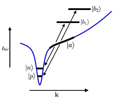
Figure 1: (Color online) Schematic showing the ideal polariton dispersion relation, and the stimulated scattering of polaritons from reservoir states, $|a\rangle$, into low-energy condensate states, $|n\rangle,|p\rangle$, and by-product states, $|b_{1}\rangle,|b_{2}\rangle$. The states can be localized in real space, and hence are indicated here as involving a range of wave vectors.

The level structure involved in Fig. 1 and Eq. (2) is that of a two-mode laser with a common level, $|a\rangle$, shared by the two modes. We outline the derivation of the dissipator $\mathcal{L}_{p}$ for this level scheme here; similar treatments can be found in Refs. Singh and Zubairy, 1980; Scully and Zubairy, 1997.

We begin by introducing the reduced density operator describing the condensates and one set of high-energy levels, $\rho_{i}=\mathrm{Tr}_{j\neq i}\,\rho$, and its matrix elements in Fock states

$$\rho_{i}=\sum\rho_{nmpq}^{\alpha_{i}\beta_{i}}\mid n\rangle\langle m\mid\otimes\mid p\rangle\langle q\mid\otimes\mid\alpha_{i}\rangle\langle\beta_{i}\mid,$$ (4)

where $n,m$ ($p,q$) denote the occupations of the first (second) condensate mode, and $\alpha_{i},\beta_{i}\in\{a,b_{1},b_{2}\}$ the occupations of the reservoir and by-product levels. These states, for exciton-exciton scattering, have either two excitons in the reservoir orbital $i$ (the state indicated by $a$) or one in a by-product orbital (the states indicated by $b_{1}$ and $b_{2}$). For exciton-phonon processes, they have either one exciton in the reservoir orbital (indicated by $a$) or a phonon in a by-product state (indicated by $b_{1}$ and $b_{2}$). We also introduce a composite object which is the sum over these reduced density operator matrix elements, $\rho_{nmpq}^{\alpha\beta}=\sum_{i}\rho_{nmpq}^{\alpha_{i}\beta_{i}}$. The reduced Hamiltonian which carries the evolution of this density matrix is

$$H_{p}=\sum_{i=1,2}g_{i}\big{(}a_{i}^{\dagger}c_{b_{i}}^{\dagger}c_{a}+c_{a}^{\dagger}c_{b_{i}}a_{i}\big{)},$$ (5)

where we based ourselves on the phonon form of Eq. (2) for notational simplicity.

The manipulationsScully and Zubairy (1997) we now present revolve around solving the following schematic relation, in the interaction picture,

$$\dot{\rho}=-i[H_{p},\rho]+\lambda_{a}\rho_{[\phi\rightarrow a]}-\gamma_{r}\rho_{[a,b_{i}\rightarrow\phi]}+(\mathcal{L}_{d}\rho).$$ (6)

The $\lambda_{a}$ term represents the replenishing of the upper level $|a\rangle$ from a vacuum state $|\phi\rangle$. This corresponds to the relaxation of laser-generated higher energy polaritons into the reservoir. The $\gamma_{r}$ term is for the decay from the $|a\rangle,|b_{i}\rangle$ levels via channels other than the condensates, e.g., spontaneous emission into outside cavity modes. Linking the replenishing and relaxation processes to a common vacuum level, $|\phi\rangle$, allows us to manipulate these $\lambda_{a},\ \gamma_{r}$ terms in rate equations, assuming that the population of that level is time-independent. The rate equations themselves correspond to the diagonal elements of the standard Lindblad forms for the transitions shown schematically in Eq. (6). In this adiabatic limit, the levels are eliminated, turning the replenishing into a term $\lambda_{a}\rho_{nmpq}^{aa}\rightarrow r\rho_{nmpq}$, with the effective pumping rate, $r$, given by

$$r=\cfrac{\lambda_{a}\gamma_{r}}{\lambda_{a}+\gamma_{r}}$$ (7)

(see Appendix A for derivation).

Second, we exploit the two different time scales associated with the processes in Eq. (6). We assume that the relaxation, proportional to $\gamma_{r}$, is much faster than the dynamics of the modes due to the action of the pumping Hamiltonian Eq. (5) and Lindblad decay, $\mathcal{L}_{d}$. This allows us to solve for the slowly varying processes, $\dot{\rho}\simeq-i[H_{p},\rho]$, on a time scale for which they appear stationary, with respect to the $\gamma_{r}$ dynamics. The matrix elements of the commutator of the composite object, $-i[H_{p},\rho]$, are given by

$$\dot{\rho}_{nmpq}^{\alpha\beta} =-i\Big{[}g_{1}\delta_{\alpha b_{1}}\sqrt{n}\rho_{n-1mpq}^{a\beta}+g_{2}\delta_{\alpha b_{2}}\sqrt{p}\rho_{nmp-1q}^{a\beta}$$ (8)

$$-g_{1}\delta_{\beta a}\sqrt{m+1}\rho_{nm+1pq}^{\alpha b_{1}}-g_{2}\delta_{\beta a}\sqrt{q+1}\rho_{nmpq+1}^{\alpha b_{2}}$$

$$+g_{1}\delta_{\alpha a}\sqrt{n+1}\rho_{n+1mpq}^{b_{1}\beta}+g_{2}\delta_{\alpha a}\sqrt{p+1}\rho_{nmp+1q}^{b_{2}\beta}$$

$$-g_{1}\delta_{\beta b_{1}}\sqrt{m}\rho_{nm-1pq}^{\alpha a}-g_{2}\delta_{\beta b_{2}}\sqrt{q}\rho_{nmpq-1}^{\alpha a}\Big{]}.\quad\quad$$

To obtain the desired equation of motion we take the trace of Eq. (8), $\sum_{\alpha,\beta=a,a;b_{1},b_{1};b_{2},b2}\dot{\rho}_{nmpq}^{\alpha\beta}=\dot{\rho}_{nmpq}$, giving a form depending on the eight components of the density operator appearing on the right-hand side. The equations-of-motion for these components are obtained by using Eq. (8) once again. This second time, we introduce the loss terms, $-\gamma_{r}\,\rho_{nmpq}^{\alpha\beta}$, and the effective pumping, $r\rho_{nmpq}\delta_{\alpha a}\delta_{\beta a}$, in the right-hand side.

The full set of equations of motion for the eight matrix elements of the traced density operator $\dot{\rho}_{nmpq}$ can thus be constructed, and assembled into three matrix equations of the form

$$\dot{R}=-MR+A.$$ (9)

Here the $M$ are $9\!\times\!9$ matrices, the $R$ are vectors formed from elements of the density matrix, in which two quanta are being passed between the reservoirs and the condensate modes in closed form, and the $A$ vectors are the driving terms (see Appendix B for explicit forms). The only non zero element, in each of the A vectors, is $r\rho_{nmpq},\,r\rho_{n-1m-1pq},\,r\rho_{nmp-1q-1}$. Solving for the three forms adiabatically, $\dot{R}=0\Rightarrow R=M^{-1}A$, and substituting the proper elements back into the traced version of Eq. (8), gives the dissipator describing the pumping:

$$\mathcal{L}_{p}\rho_{nmpq}=-r\frac{\big{(}g_{1}^{2}(n-m)+g_{2}^{2}(p-q)\big{)}^{2}+\big{(}g_{1}^{2}(n+m+2)+g_{2}^{2}(p+q+2)\big{)}\gamma_{r}^{2}}{\big{(}g_{1}^{2}(n-m)+g_{2}^{2}(p-q)\big{)}^{2}+2\gamma_{r}^{2}\big{(}g_{1}^{2}(n+m+2)+g_{2}^{2}(p+q+2)\big{)}+\gamma_{r}^{4}}\rho_{nmpq}$$

$$+\frac{2r\gamma_{r}^{2}g_{1}^{2}\sqrt{nm}}{\big{(}g_{1}^{2}(n-m)+g_{2}^{2}(p-q)\big{)}^{2}+2\gamma_{r}^{2}\big{(}g_{1}^{2}(n+m)+g_{2}^{2}(p+q+2)\big{)}+\gamma_{r}^{4}}\rho_{n-1m-1pq}$$

$$+\frac{2r\gamma_{r}^{2}g_{2}^{2}\sqrt{pq}}{\big{(}g_{1}^{2}(n-m)+g_{2}^{2}(p-q)\big{)}^{2}+2\gamma_{r}^{2}\big{(}g_{1}^{2}(n+m+2)+g_{2}^{2}(p+q)\big{)}+\gamma_{r}^{4}}\rho_{nmp-1q-1}.$$ (10)

Note that $g_{1,2}$ are squared in our result; the scattering rates into the condensates depend on the probability densities of the condensate wavefunctions at the reservoir, $|\phi_{1,2}(r_{o})|^{2}$, via Eq. (3). Setting $n=m,\,p=q$ in Eq. (II.1) gives the equation-of-motion for the population distribution,

$$\dot{P}_{np}=\; \gamma n_{c}\Bigg{[}\dfrac{\alpha_{1}n}{\alpha_{1}n+\alpha_{2}(p+1)+n_{s}}P_{n-1p}+\dfrac{\alpha_{2}p}{\alpha_{1}(n+1)+\alpha_{2}p+n_{s}}P_{np-1}-\dfrac{\alpha_{1}(n+1)+\alpha_{2}(p+1)}{\alpha_{1}(n+1)+\alpha_{2}(p+1)+n_{s}}P_{np}\Bigg{]}$$

$$\;\;+\gamma\Big{[}(n+1)P_{n+1p}+(p+1)P_{np+1}-(n+p)P_{np}\Big{]},$$

where we have added the standard Lindblad damping termsScully and Zubairy (1997) for radiation from the condensate modes, assumed to decay at equal rates $\gamma$ to simplify the notation. Here we have also introduced a dimensionless pumping parameter, $n_{c}=r/2\gamma$, a pump saturation parameter, $n_{s}=\gamma_{r}^{2}/[4(g_{1}^{2}+g_{2}^{2})]$, and the ratios $\alpha_{1(2)}=g_{1(2)}^{2}/(g_{1}^{2}+g_{2}^{2})$. This is the generalization, to the two-mode case, of the pump parametrization used in Ref. Whittaker and Eastham, 2009. Note that the pumping in Eq. (II.1) is saturable: the gain is reduced as the occupation increases, due to the occupation numbers in the denominators. Furthermore it includes a gain competition effect, with the growth rate of one mode reduced by the occupation of the other. This arises from the common level, $|a\rangle$.

We can find a steady-state solution by requiring that the growth of an occupation probability due to pumping matches its decay due to loss. The first two terms on the first line of Eq. (II.1) correspond to transitions into the state of $n,p$ particles caused by the pumping, while the final term on the second line corresponds to transitions out of this state caused by the loss. Similarly, the final term on the first line of Eq. (II.1) corresponds to transitions out of the state $n,p$ caused by the pumping, while the first two terms on the second line correspond to transitions into this state caused by the loss. We can find a steady-state solution by requiring that either one of these sets of rates balances. Such a detailed balance conditionCarmichael and Walls (1974) ensures that the other set also balances, and that there is no net flow of probability to higher or lower occupation numbers. Specifically, in Eq. (II.1), it corresponds to the steady-state equation splitting in two identical conditions

$$P_{np}=\dfrac{n_{c}}{n+p}\Bigg{(} \cfrac{\alpha_{1}nP_{n-1p}}{\alpha_{1}n+\alpha_{2}(p+1)+n_{s}}$$ (12)

$$+\dfrac{\alpha_{2}pP_{np-1}}{\alpha_{1}(n+1)+\alpha_{2}p+n_{s}}\Bigg{)}.$$

Note that in this single-reservoir model the gain competition leads to single-mode behavior: except for the point $\alpha_{1}=\alpha_{2}$ the population distribution obtained from Eq. (12) peaks when either $n=0$ or $p=0$. Multimode behavior will become possible when more than one reservoir is introduced, reducing the impact of the gain competition.

We note that in the single-mode case, the population dynamics, Eq. (II.1), and distribution, Eq. (12) correspond to a standard laser-like saturable pumping. In particular, Eq. (12) reduces to

$$P_{n}=\frac{n_{c}}{n+n_{s}}P_{n-1},$$ (13)

which is Eq. (11.2.14) in Ref. Scully and Zubairy, 1997; see also Eq. (4) in Ref. Whittaker and Eastham, 2009. A similar recurrence relation has been obtained by Laussy et al.Laussy et al. (2004) for a model of a single condensate mode coupled to a bosonic reservoir. Note that their Eq. (4) can be put in the form of Eq. (13) by expanding their denominator to first order in the occupation number.

We can obtain an approximate solution to the recurrence relation, Eq. (12), by dropping the $+1$s in the denominators, replacing the occupation numbers with continuous variables, and approximating $P_{n-1p}\rightarrow P_{(n,p)}-1\cdot\partial_{n}P_{(n,p)}$ and $P_{np-1}\rightarrow P_{(n,p)}-1\cdot\partial_{p}P_{(n,p)}$. The solution of the differential equation thereby obtained is the multivariate Gaussian

$$P_{(n,p)}\propto\mathrm{exp}\Bigg{(}-\frac{(n+p)^{2}}{2n_{c}}+\frac{\alpha_{1}n_{c}-n_{s}}{\alpha_{1}n_{c}}n\\ +\frac{\alpha_{2}n_{c}-n_{s}}{\alpha_{2}n_{c}}p\Bigg{)}.$$ (14)

II.2 Many reservoirs pumping many modes

We now generalize the above results to allow many different reservoirs to pump many different condensate modes. The Hamiltonian for scattering from each of these reservoirs is Eq. (2), generalized to many condensate modes. We now use $g_{ij}$ to denote the matrix element for a transition from one of the initial $(|a\rangle)_{i}$ levels in reservoir $i$ into a by-product state $(|b_{j}\rangle)_{i}$ in that reservoir, and a polariton in a condensate mode $j$. Note that each reservoir generally involves many high-energy states, as in Eq. (2), whose matrix elements for scattering into a particular condensate mode are all supposed to be approximately equal. We further assume that the different reservoirs are independent, except for their coupling via the condensates. From the forms of the matrix elements, Eq. (3), we see that the first assumption is valid when the reservoirs are regions of space that are small enough for the variation in the condensate wavefunctions across each to be ignored. The second condition requires that the reservoirs are large compared with the mean free path of the high-momentum excitons above the bottleneck.

As an aperçu,Racine (2013) the generalization to many reservoirs means that the full high-energy subspace is subdivided into blocks. The reservoirs and by-products density matrix elements, defined after Eq. (4), now carry indices for each reservoir, $\rho_{..}^{\alpha_{1}\beta_{1}\alpha_{2}\beta_{2}..\alpha_{i}\beta_{i}..}$, and the matrices $M$ become Kronecker sums, $M=\sum_{i}I\otimes..\otimes M_{i}\otimes..\otimes I$. But the assumed independence of the different reservoirs means that the pumping terms ($A$ vectors) appear in each subspace, and the result is that the dissipator for pumping by many reservoirs is the sum of dissipators for individual reservoirs. The generalization to many condensates means that each $M_{i}$ associating the $i^{th}$ reservoir with $v$ condensates is an $(1\!+\!v)^{2}\!\times\!(1\!+\!v)^{2}$ matrix. The forms of these matrices, however, allow the relevant elements oftheir inverses to be obtained [most of the terms in the cofactors and the determinants which form $(M_{i})^{-1}_{i1}\!=\!\tfrac{(C_{i})_{i1}}{|M_{i}|}$ cancel], and the final result is a direct generalization of Eq. (II.1) :

$$\mathcal{L}_{p}\rho_{n_{1}\,n_{2}\;..}^{m_{1}m_{2}..}=\sum_{i}r_{i}\Bigg{[}\sum_{j} \dfrac{2\gamma_{r}^{2}g_{ij}^{2}\sqrt{n_{j}m_{j}}\rho_{n_{1}\,n_{2}\;...n_{j}-1..}^{m_{1}m_{2}..m_{j}-1..}}{\big{(}\sum_{k}g_{ik}^{2}(n_{k}-m_{k})\big{)}^{2}+2\gamma_{r}^{2}\sum_{k}g_{ik}^{2}(n_{k}+m_{k}+2)-4\gamma^{2}_{r}g_{ij}^{2}+\gamma_{r}^{4}}$$ (15)

$$-\dfrac{\big{(}\sum_{j}g_{ij}^{2}(n_{j}-m_{j})\big{)}^{2}+\gamma_{r}^{2}\sum_{j}g_{ij}^{2}(n_{j}+m_{j}+2)}{\big{(}\sum_{j}g_{ij}^{2}(n_{j}-m_{j})\big{)}^{2}+2\gamma_{r}^{2}\sum_{j}g_{ij}^{2}(n_{j}+m_{j}+2)+\gamma_{r}^{4}}\rho_{n_{1}\,n_{2}\;..}^{m_{1}m_{2}..}\Bigg{]}$$

($\rho_{n_{1}\,n_{2}\;..}^{m_{1}m_{2}\;..}\equiv\langle n_{1},n_{2},..|\rho|m_{1},m_{2},..\rangle$, with $n_{j}$ and $m_{j}$ occupation numbers of the condensate modes). Note that the growth of condensate $j$ due to reservoir $i$ depends on the (squared) magnitude of the condensate orbital at the position of that reservoir, via the matrix element $g_{ij}$, as well as the pump rate for that reservoir, $r_{i}$. Since the reservoir $i$ is now feeding many condensate modes, the gain is reduced according to all their occupations, giving rise to the sums over condensate modes in the second terms of the denominators.

The generalization of the dimensionless pumping parameter for reservoir $i$, introduced above, is $n_{i}^{c}=r_{i}/2\gamma$, while the pump saturation parameter becomes $n_{i}^{s}=\gamma_{r}^{2}/(4\sum_{j}g_{ij}^{2})$, and the normalized transition strengths become

$$\alpha_{ij}=g_{ij}^{2}/\sum_{k}g_{ik}^{2}.\vspace{0.5in}$$ (16)

Finally, the population dynamics equation (II.1) now reads

$$\dot{P}_{n_{1}n_{2}..} =\gamma\sum_{i}n_{i}^{c}\sum_{j}\Big{[}\frac{\alpha_{ij}n_{j}P_{n_{1}n_{2}..n_{j}-1..}}{\sum_{k}\alpha_{ik}(n_{k}+1)-\alpha_{ij}+n_{i}^{s}}$$

$$-\frac{\alpha_{ij}(n_{j}+1)P_{n_{1}n_{2}..}}{\sum_{k}\alpha_{ik}(n_{k}+1)+n_{i}^{s}}\Big{]}$$

$$+\gamma\sum_{j}\Big{[}(n_{j}+1)P_{n_{1}n_{2}..n_{j}+1..}-n_{j}P_{n_{1}n_{2}..}\Big{]}.$$

We have found an approximate steady-state solution of this equation, for the special case where the coupling ratios among the $u$ reservoirs and $v$ condensates obey $\alpha_{ii+j}=\beta_{j},i=1,2..u,j=0,1,2,..,v-1$, with the index $i+j$ treated circularly around $v$, and where all the $n_{i}^{s},n_{i}^{c}$ are the same. The solution, valid to the extent that Eq. (21) holds, is the multivariate Gaussian

$$P {}_{(n_{1},n_{2},..)}\propto\mathrm{exp}\Bigg{[}\!\!-\frac{1}{2}\begin{pmatrix}n_{1}&n_{2}&..\end{pmatrix}\cdot\mathbb{S}\cdot\begin{pmatrix}n_{1}\\ n_{2}\\ ..\end{pmatrix}+\mathbb{Z}\cdot\begin{pmatrix}n_{1}\\ n_{2}\\ ..\end{pmatrix}\!\Bigg{]}$$

with

$$\mathbb{S}=\begin{pmatrix}\frac{\sum_{i}\beta_{i}^{2}}{n_{c}}&\frac{\sum_{i,j\neq i}\beta_{i}\beta_{j}}{n_{c}}&..\\ \frac{\sum_{i,j\neq i}\beta_{i}\beta_{j}}{n_{c}}&\frac{\sum_{i}\beta_{i}^{2}}{n_{c}}&..\\ ..&..&..\end{pmatrix}$$ (19)

and

$$\mathbb{Z}=\begin{pmatrix}\tfrac{n_{c}-n_{s}}{n_{c}}&\tfrac{n_{c}-n_{s}}{n_{c}}&..\end{pmatrix}.$$ (20)

The validity of Eq. (II.2) can be seen by substituting it into the continuous version of Eq. (II.2). For the case of two condensates and two reservoirs this gives

$$0\approx\beta_{o}\beta_{1}\!\Bigg{(}\cfrac{(\beta_{1}\!-\!\beta_{o})(n\!-\!p)}{\beta_{o}n\!+\!\beta_{1}p\!+\!n_{s}}+\cfrac{(\beta_{o}\!-\!\beta_{1})(n\!-\!p)}{\beta_{1}n\!+\!\beta_{o}p\!+\!n_{s}}\Bigg{)}.$$ (21)

III Coherence functions

III.1 Low-energy Hamiltonian

We now consider how the dissipative dynamical model, described above, may be further developed, and used to calculate the dynamical characteristics of a multimode polariton condensate. In particular, we consider the calculation of time-dependent first and second order coherence functions. To keep the notation manageable we consider explicitly a two-mode condensate; the formulation is such that the generalization is reasonably straightforward.

The first step is to introduce the Hamiltonian dynamics of the condensate modes. In particular, we include the polariton-polariton interactions. The underlying interaction Rochat et al. (2000) is predominantly due to the exchange terms in the Coulomb and radiative couplings (phase-space filling), so that its range is on the order of the Bohr radius. It should thus, in the present low-energy theory, be understood to be a contact interaction, $V(r)=V_{0}\delta^{d}(r)$, with matrix element $\mu_{ijkl}=V_{0}\int d^{d}r\psi^{\ast}_{i}(r)\psi_{j}(r)\psi^{\ast}_{k}(r)\psi_{l}(r)$. The low-energy Hamiltonian is then

$$H=\sum_{i=1,2}\omega_{i}a^{\dagger}_{i}a_{i}+\tfrac{1}{2}\sum_{ijkl}\mu_{ijkl}a^{\dagger}_{i}a_{j}a^{\dagger}_{k}a_{l},$$ (22)

where $\omega_{i}$ are the single-particle energies. This form is obtained by diagonalizing the single-particle Hamiltonian, so that $a_{i}$ is the annihilation operator in a single orbital. An example of this procedure, diagonalizing the Hamiltonian for a double-well system by eliminating the hopping term, is described in Sec. IV.

In order to render the general interacting bosonic Hamiltonian, Eq. (22), tractable, we consider the case in which there is some trapping potential creating localized single-particle orbitals for the polaritons. We furthermore assume the strong-trapping limit, where the energy separation between the orbitals, $\omega_{i}-\omega_{j}$, is large compared with the interaction energy (of order $V_{0}n$ for an overall condensate density $n$). We will therefore neglect the parts of the interaction which transfer particles between different orbitals, i.e., non resonant scattering processes between condensates in different modes. This makes the problem tractable since the equation of motion becomes diagonal in Fock space. It is consistent with the semiclassical limit of the equations of motion, in which such processes give rise to rapidly oscillating terms.Eastham (2008) However, the nonlinear terms which conserve the number of particles in each orbital must be retained, since their effects are not suppressed by the differences in single-particle energies. For the two-mode problem we will thus take for the interaction Hamiltonian the form

$$H_{(NL)}=\kappa(a_{1}^{\dagger}a_{1})^{2}+\kappa(a_{2}^{\dagger}a_{2})^{2}+\eta a_{1}^{\dagger}a_{1}a_{2}^{\dagger}a_{2},$$ (23)

including the Fock space diagonal interactions within each mode (strength $\kappa$) and between the modes (strength $\eta$). However, the Bogoliubov or parametric scattering terms, such as $a_{1}^{\dagger}a^{\dagger}_{1}a_{2}a_{2}$, are neglected. Since the single-particle energies are just energy shifts in the following they will often be dropped. The form of the equation of motion, (1), we consider is thus

$$\dot{\rho}=\mathcal{L}_{p}\rho \ -\ \tfrac{\gamma}{2}\bigl{(}(a_{1}^{\dagger}a_{1}+a_{2}^{\dagger}a_{2})\rho+\rho(a_{1}^{\dagger}a_{1}+a_{2}^{\dagger}a_{2})$$ (24)

$$\ -\ 2a_{1}\rho a_{1}^{\dagger}-2a_{2}\rho a_{2}^{\dagger}\bigr{)}-i[H_{(NL)},\rho].$$

We note that the form of the interactions in Eq. (23) do not enter into the equation for the population dynamics, Eqs. (II.1, II.2), since $H_{(NL)}$ commutes with the diagonal elements of $\rho$. Their role will be primary however in the calculation of coherence functions below.

III.2 First-order coherence functions

A key application of the equation of motion, (1), is to calculate the linewidths of the emission from the individual condensate modes. Whittaker and Eastham (2009) Equivalently, one can consider the first-order coherence function of the emission from mode 1, for example, $g^{(1)}(\tau)\propto\langle a_{1}^{\dagger}(\tau)a_{1}(0)\rangle$. By the Wiener-Khinchin theorem, the Fourier transform of this correlation function gives the power spectrum of the electromagnetic field, i.e., the emission spectrum.Loudon (2000) Such spectra have been studied experimentally.Love et al. (2008) The linewidth has been shown to be generated by the interplay between interactions and the polariton number fluctuations, discussed above, which together imply energy fluctuations.

The first-order coherence function may be calculated from the equation of motion for the reduced density matrix, by exploiting a form of the quantum regression theorem.Scully and Zubairy (1997); Swain (1981) Thus, the two-time correlation function $\langle a_{1}^{\dagger}(\tau)a_{1}(0)\rangle$ is the expectation value $\langle a_{1}^{\dagger}\rangle=\operatorname{Tr}a_{1}^{\dagger}\rho^{\prime}$, with a density operator $\rho^{\prime}(\tau)=e^{\mathcal{L}\tau}\rho^{\prime}(0)$ obtained by evolving $\rho^{\prime}(0)=a_{1}\rho(0)$ according to Eq. (1). In this form the regression theorem holds provided the system-reservoir coupling is weak, so that the full density operator factorizes. This is already implicit in our model for pumping and decay. We note that there is also a stronger version of the quantum regression theorem, which relates the equations of motion for $n$-time correlation functions to those for $m$-time ones.Scully and Zubairy (1997); Ford and O’Connell (1996) This is not useful here, because the nonlinearities mean that $\langle a_{1}(t)\rangle$, for example, does not obey a closed set of linear equations of motion.

To implement this quantum regression approach, we introduce the distributionWhittaker and Eastham (2009) $u_{np}(\tau)=\sqrt{n}\rho^{\prime}_{n-1npp}(\tau)$ , so that

$$g^{(1)}(\tau)\propto\langle a_{1}^{\dagger}\rangle=\sum_{n,p}u_{np}(\tau).$$ (25)

The initial condition for the evolution is

$$u_{np}(0)=\langle n,p|a^{\dagger}_{1}a_{1}\rho(0)|n,p\rangle=nP^{ss}_{np},$$ (26)

where the steady-state population distribution $P^{ss}_{np}$ is obtained from Eq. (II.2) [or more generally Eq. II.2]. From Eq. (1) we find the equation of motion for $u_{np}$,

$$\dot{u}_{np}=\gamma\sum_{i=1,2}n^{c}_{i} \bigg{[}\dfrac{\alpha_{i1}n}{\alpha_{i1}(n-\frac{1}{2})+\alpha_{i2}(p+1)+n^{s}_{i}}u_{n-1p}$$

$$+\dfrac{\alpha_{i2}p}{\alpha_{i1}(n+\frac{1}{2})+\alpha_{i2}p+n^{s}_{i}}u_{np-1}$$

$$-\dfrac{\alpha_{i1}(n+\frac{1}{2})+\alpha_{i2}(p+1)}{\alpha_{i1}(n+\frac{1}{2})+\alpha_{i2}(p+1)+n^{s}_{i}}u_{np}\bigg{]}$$

$$+\gamma\bigg{[}nu_{n+1p} +(p+1)u_{np+1}-\big{(}(n-\frac{1}{2})+p\big{)}u_{np}\bigg{]}$$

$$+i\big{[}\kappa(2n- 1)+\eta p\big{]}u_{np}.$$ (27)

We have neglected terms $\mathcal{O}(\frac{n}{n_{s}}\cdot n)$, since $n_{s}\gg\langle n\rangle$ for our system. The solution to Eq. (III.2), with the appropriate initial condition, Eq. (26), gives the first-order coherence function via Eq. (25). For up to several hundreds of particles, $\dot{u}_{np}$ can be integrated numerically to obtain $g^{(1)}(\tau)$.

In the single-mode case, an expansion based on the one mode equivalent of Eq. (III.2) was solved analytically in Ref. Whittaker and Eastham, 2009. A Kubo formHamm (2005); Kubo (1954) was reached which incorporates the interaction and the slower Schawlow-Townes broadening. Within each term both a Lorentzian and a Gaussian lineshape can be obtained depending on which limit is applied, i.e., motional broadening and the static limit. For multimode condensation, we could not reach a simple analytic formula for the first-order correlation function and we therefore resort to the semianalytic approaches presented below.

III.3 First-order coherence: Fokker-Planck approach

To make Eq. (III.2) tractable more widely, we recast it in the form of a soluble partial differential equation. This process follows the derivation of the Fokker-Planck equation for a one-step Markov process.Kampen (2007) It involves approximating the occupation numbers by continuous variables, and expanding the finite-difference operators in terms of differentials (Kramers-Moyal expansion).

We first introduce step operators $\mathbb{E}_{n,p}$, whose action, for example, is $\mathbb{E}_{n}nu_{np}=(n+1)u_{n+1p}$. This allows us to rewrite Eq. (III.2) as

$$\dot{u}_{np}= (\mathbb{E}_{n}^{-1}-1,\mathbb{E}_{p}^{-1}-1)\cdot\big{[}(q_{n},q_{p})u_{np}\big{]}$$ (28)

$$+\ (\mathbb{E}_{n}-1,\mathbb{E}_{p}-1)\cdot\big{[}(r_{n},r_{p})u_{np}\big{]}$$

$$+\ (h+s)u_{np}$$

where

$$q_{n,p}=\ \gamma n_{c}\Big{(}\frac{\beta_{o,1}}{D_{o}}+\frac{\beta_{1,o}}{D_{1}}\Big{)}(n,p+1)$$ (29)

$$r_{n}=\ \gamma(n-1),\quad r_{p}=\ \gamma\,p.$$ (30)

The first two lines in Eq. (28) correspond to the master equation for a one-step stochastic process, such as nearest-neighbor transitions in two dimensions, with $u_{np}$ interpreted as a probability, and $q_{n,p},r_{n,p}$ transition rates. These contributions conserve the sum of $u$, and alone would lead to the Fokker-Planck (i.e., continuity) equation in the continuous limit. A nonconserving term proportional to

$$h=\frac{\gamma n_{c}}{2}\Big{(}\frac{\beta_{o}}{D_{o}}+\frac{\beta_{1}}{D_{1}}\Big{)}-\frac{\gamma}{2},$$ (31)

remains when the gain and loss terms in Eq. (III.2) are recast in this way. Here $\beta_{o}=\alpha_{11},\alpha_{22}$ and $\beta_{1}=\alpha_{12},\alpha_{21}$, and

$$D_{o,1}=\beta_{o,1}(n+\tfrac{1}{2})+\beta_{1,o}(p+1)+n_{s}.$$ (32)

The interactions, also, lead to a non-conserving term, proportional to

$$s=i\big{[}\kappa(2n-1)+\eta p\big{]}.$$ (33)

We then Taylor-expand the step operators $\mathbb{E}_{n,p}^{\pm 1}\rightarrow 1\pm\partial_{n,p}+\frac{1}{2}\partial_{n,p}^{2}$, and obtain the continuous approximation

$$\dot{u}_{(n,p)}= (h+s)u_{(n,p)}+\nabla\cdot[(\mathbf{r}-\mathbf{q})u_{(n,p)}]$$

$$+\tfrac{1}{2}\nabla^{2}\cdot[(\mathbf{r}+\mathbf{q})u_{(n,p)}]$$

$$= (h+s)u_{(n,p)}$$ (34)

$$+\nabla\cdot\{[\mathbf{r}-\mathbf{q}+\tfrac{1}{2}\nabla\odot(\mathbf{r}+\mathbf{q})]u_{(n,p)}$$

$$\qquad+\tfrac{1}{2}(\mathbf{r}+\mathbf{q})\odot\nabla u_{(n,p)}\},$$

where $\mathbf{r}=(r_{n},r_{p}),\mathbf{q}=(q_{n},q_{p}),\nabla=(\partial_{n},\partial_{p})$, $\nabla^{2}=(\partial^{2}_{n},\partial^{2}_{p})$, and $\odot$ denotes elementwise multiplication. We notice that the conserving part of Eq. (34) is a convection equation in the occupation number space, with a position-dependent drift velocity, given by the prefactor of $u$ inside the divergence, and a diffusion coefficient, given by the prefactor of $\nabla u$. The remaining terms, proportional to $h+s$, cause the integral of $\dot{u}$ to be non-zero. They induce the decay in magnitude of $u$, and hence are responsible for decoherence and the finite linewidth, according to Eq. (25). The standard Schawlow-Townes linewidth arises from the term proportional to $h$, while the interaction broadening arises from that proportional to $s$.

Equation (34), like the Fokker-Planck equation, is soluble when $h$, $s$, and the drift coefficients are at most linear functions of the occupation numbers, and the diffusion coefficients are constants. We therefore expand these coefficients appropriately in Taylor series around the mean of the initial conditions, $n_{l}=\frac{\langle nu_{o}\rangle}{\langle u_{o}\rangle}$, $p_{l}=\frac{\langle pu_{o}\rangle}{\langle u_{o}\rangle}$. For simplicity we also neglect the quadratic terms in the expansion of $\mathbf{r}+\mathbf{q}$, which would contribute a small linear term to the drift coefficient.

We define $n^{\prime}=n-n_{l}$, and introduce the reciprocal representation $g=\iint e^{-i(k_{1},k_{2})\cdot(n^{\prime}\!,p^{\prime})}u_{(n^{\prime}\!,p^{\prime})}\mathrm{d}n^{\prime}\mathrm{d}p^{\prime}$. The appropriately linearized form of Eq. (34) is then

$$\dot{g}+\sum_{j}\big{(}a_{j}+\sum_{i} b_{ij}k_{i}\big{)}\partial_{k_{j}}g=$$ (35)

$$cg+\sum_{i}d_{i}k_{i}g+\sum_{i}e_{i}k_{i}^{2}g,$$

with coefficients

$$A= -i\nabla(h+s)|_{n_{l},p_{l}}$$ (36)

$$B= \left.\begin{pmatrix}\nabla(r_{n}-q_{n})\\ \nabla(r_{p}-q_{p})\end{pmatrix}\right|_{n_{l},p_{l}}$$ (37)

$$c= h|_{n_{l},p_{l}}$$ (38)

$$D= i\big{(}r_{n}-q_{n}+\tfrac{1}{2}\partial_{n}(r_{n}+q_{n}),$$ (39)

$$\quad\quad r_{p}-q_{p}+\tfrac{1}{2}\partial_{p}(r_{p}+q_{p})\big{)}\big{|}_{nl,pl}$$

$$E= -\frac{1}{2}\left.\begin{pmatrix}r_{n}+q_{n}&0\\ 0&r_{p}+q_{p}\end{pmatrix}\right|_{n_{l},p_{l}},$$ (40)

where $D=(d_{1},d_{2})$, etc.. The origins of the various terms in Eqs. (36)–(39) can be seen in Eq. (34); note there are contributions from both $r-q$ and $r+q$ to the lowest-order drift matrix $D$, from the two terms on the second-to-last line of Eq. (34). At $k_{1,2}=0$, the solution of Eq. (35) shall give $g^{(1)}(\tau)$.

We solve Eq. (35) using the method of characteristics Kampen (2007) to reduce it to a set of coupled ordinary differential equations. The characteristic equation is $\dot{K}=A+KB$, which may be solved in the eigenbasis of $B$, $\mathbb{B}=P^{\,-1}BP$, where $P$ is the eigenvector matrix of $B$, before transforming back to the original basis. This gives

$$K_{o}=-AB^{-1}+(AB^{-1}+K)e^{-B\tau},$$ (41)

where $K_{0}=K(\tau=0)$. Note that the origin $\tau=0$ is significant and the constant $-AB^{-1}$ cannot be dropped. We then obtain

$$g=g_{o}(K_{o})\,\mathrm{exp}\Big{[}c\tau+D\!\int_{0}^{\tau}K\mathrm{d}t^{\prime}+\int_{0}^{\tau}KE\tilde{K}\mathrm{d}t^{\prime}\Big{]},$$ (42)

using $\tilde{K}$ to denote the transpose of $K$. The first integral inside the exponential is

$$\int_{0}^{\tau}K\mathrm{d}t^{\prime}\ =-AB^{-1}\tau+(K_{o}+AB^{-1})B^{-1}(e^{B\tau}\!-\!I)$$

$$=- AB^{-1}\tau+(AB^{-1}+K)B^{-1}(I\!-\!e^{-B\tau}),$$ (43)

which at $K=0$ gives

$$\zeta(\tau)=-DAB^{-1}\tau+DAB^{-1}B^{-1}(I\!-\!e^{-B\tau}).$$ (44)

The second integral is solved in a similar fashion, only in this case the result depends explicitly on the eigenvalues and eigenvectors of $B$. We define $E_{p}=P^{\,-1}E\tilde{P}^{\,-1}$ and obtain

$$\xi(\tau)=AB^{-1}E\tilde{B}^{-1}\tilde{A}\tau$$

$$\quad-\Big{(}AB^{-1}B^{-1}(I\!-\!e^{-B\tau})E\tilde{B}^{-1}\tilde{A}+\mathrm{T.c.}\Big{)}+AB^{-1}P$$

$$\quad\times\Big{[}\sum_{ij}\hat{\imath}\otimes\hat{\jmath}\frac{E_{p\,ij}}{\mathbb{B}_{ii}\!+\!\mathbb{B}_{jj}}(I\!-\!e^{-(\mathbb{B}_{ii}+\mathbb{B}_{jj})\tau})\Big{]}\tilde{P}\tilde{B}^{-1}\tilde{A}.$$ (45)

The tensor product $\hat{\imath}\otimes\hat{\jmath}$ with unit vectors $\hat{\imath},\hat{\jmath}$ generates a matrix with all zeros except at position $ij$. We finally obtain the solution

$$g^{(1)}(\tau)=g_{o}(\tau)\,\mathrm{exp}\big{(}c\tau+\zeta(\tau)+\xi(\tau)\big{)}.$$ (46)

The function $g_{o}(\tau)$ is related to the transform of $u_{np}(0)$, given by Eq. (26),

$$g_{o}(\tau)=\Big{(}\int e^{-iK^{\prime}_{o}\cdot(n,p)}nP_{(n,p)}\mathrm{d}n\,\mathrm{d}p\Big{)}\mathrm{exp}(iK^{\prime}_{o}\cdot(n_{l},p_{l})),$$ (47)

where $K^{\prime}_{o}=-AB^{-1}(I-e^{-B\tau})$ is $K_{o}$ at $K(\tau)=0$. We also shifted the transform by the linearization points, $n^{\prime}$ $=$ $n$ $-$ $n_{l}$, $p^{\prime}$ $=$ $p$ $-$ $p_{l}$, such that it is consistent with the rest of the solution. The coefficients, Eqs. (36 - 40), can be obtained analytically, while the diagonalization of $B$ and integral in $g_{0}$ are performed numerically.

III.4 First-order coherence: static limit

For sufficiently short timescales the gain and loss processes will not change the occupation numbers of the condensate orbitals. We can therefore calculate $g^{(1)}(\tau)$ allowing only for the effects of the nonlinear Hamiltonian, Eq. (23). This is the static-limit calculation previously discussed for the single-mode case.Whittaker and Eastham (2009) The time scale over which it is valid is the time scale for intensity fluctuations, given by the decay of $g^{(2)}(t)$; due to critical slowing down this timescale becomes long close to threshold, and most of the decay of $g^{(1)}(\tau)$ is captured correctly. For the two-mode case we find

$$|g_{s}^{(1)}(\tau)| =\Big{|}\operatorname{Tr}\sum_{np}a_{1}^{\dagger}e^{-iH_{(NL)}\tau}\Big{(}P_{np}\,a_{1}|n,p\rangle\langle n,p|\Big{)}$$ (48)

$$\qquad\quad\qquad\qquad\qquad\qquad\qquad\qquad\times e^{iH_{(NL)}\tau}\Big{|}$$

$$\propto\Big{|}\iint\!P_{(n,p)}e^{i(2\kappa n+\eta p)\tau}\,\mathrm{d}n\,\mathrm{d}p\;\Big{|},$$

where in the second line we have approximated a factor of $n$ inside the integral as a constant and treated the occupation numbers as continuous. Due to the cutoff in $P_{(n,p)}$ the integral will be performed numerically. Notice that the kernel in the integral indeed corresponds to the interaction term proportional to $s$ in Eq. (III.2); all the other dynamics is neglected.

III.5 Coherence of Josephson oscillations

The approaches described above for the first-order coherence function can be generalized to calculate higher-order correlation functions. An interesting example is the second-order cross-correlation function $g^{J}(\tau)\propto\langle a_{1}^{\dagger}(\tau)a_{2}(\tau)a_{2}^{\dagger}a_{1}\rangle$. This function characterizes the coherence of the intensity oscillations, caused by the beating between the different emission frequencies in a multimode condensate. They can be interpreted as a form of Josephson oscillation. Leggett (2001)

To motivate the consideration of the correlation function $g^{J}(\tau)$ we consider the mean-field limit where the creation and annihilation operators can be treated as classical oscillating variables, $a_{1,2}(t)\to\sqrt{n_{1,2}}e^{i(\omega_{1,2}t+\phi_{1,2})}$, in other words the eigenvalues of coherent states, $|\alpha_{1,2}\rangle$. Leggett (2001); Scully and Zubairy (1997) For two orbitals with amplitudes $c_{1},c_{2}$ at a point $r$, the density or intensity is $n=(c_{1}a_{1}^{\dagger}+c_{2}a_{2}^{\dagger})(c_{1}a_{1}+c_{2}a_{2})$. Thus, in that theory, there is an oscillating contribution to the intensity, proportional to

$$\cos[(\omega_{1}-\omega_{2})t+\phi_{1}-\phi_{2}].$$ (49)

The intensity oscillations are not zero in the mean-field theory because it assumes a well-defined phase for the condensates, and hence a well-defined phase difference between them. However, in the strong-trapping limit considered here there are no terms in the Hamiltonian which fix this relative phase, and the averaged intensity does not oscillate, $\langle a_{1}^{\dagger}(\tau)a_{2}(0)\rangle=0$. Even in the absence of phase-fixing terms in the Hamiltonian, however, a phase would arise in each member of an ensemble, i.e., a single run of an experiment, due to spontaneous symmetry breaking. The fluctuations of the phases between members of the ensemble account for the vanishing of the oscillations on average. We can nonetheless study how the oscillations in each member behave, by considering the correlation function of the intensity,

$$\langle n(\tau)n(0)\rangle=\langle (a_{1}^{\dagger}(\tau)+a_{2}^{\dagger}(\tau))(a_{1}(\tau)+a_{2}(\tau))$$

$$\;\times(a_{1}^{\dagger}+a_{2}^{\dagger})(a_{1}+a_{2})\rangle,$$ (50)

and in particular the component at the beat frequency $\langle a_{1}^{\dagger}(\tau)a_{2}(\tau)a_{2}^{\dagger}a_{1}\rangle$. (We omit the amplitudes $c_{1,2}$ above for notational simplicity.)

The calculation of $g^{J}(\tau)$ closely parallels that of the first-order coherence. We again use the quantum regression theorem, so that $g^{J}(\tau)$ is the average $\langle a_{1}^{\dagger}a_{2}\rangle$, with the density operator obtained by evolving $a_{2}^{\dagger}a_{1}\rho(0)$ over the time $\tau$. We introduce the distribution

$$u_{np}^{J}=\sqrt{n}\sqrt{p+1}\,\rho^{\prime}_{n-1np+1p}(\tau),$$ (51)

such that $g^{J}(\tau)=\sum_{n,p}u_{np}^{J}$. The initial condition is $u_{np}^{J}(0)=n(p+1)\,P_{np}^{ss}$, and the evolution obeys

$$\dot{u}^{J}_{np}=\gamma\sum_{i} n^{c}_{i}\bigg{[}\frac{\alpha_{i1}n}{\alpha_{i1}(n-\frac{1}{2})+\alpha_{i2}(p+\frac{3}{2})+n^{s}_{i}}u^{J}_{n-1p}$$

$$\quad+\frac{\alpha_{i2}(p+1)}{\alpha_{i1}(n+\frac{1}{2})+\alpha_{i2}(p+\frac{1}{2})+n^{s}_{i}}u^{J}_{np-1}$$

$$\quad-\frac{\alpha_{i1}(n+\frac{1}{2})+\alpha_{i2}(p+\frac{3}{2})}{\alpha_{i1}(n+\frac{1}{2})+\alpha_{i2}(p+\frac{3}{2})+n^{s}_{i}}u^{J}_{np}\bigg{]}$$

$$+\gamma\bigg{[}n u^{J}_{n+1p}+(p+1)u^{J}_{np+1}-\big{(}n+p\big{)}u^{J}_{np}\bigg{]}$$ (52)

$$+\>i\Big{(}\kappa (2n-1)-\kappa(2p+1)+\eta(-n+p+1)\Big{)}u^{J}_{np}.$$

The static limit can be calculated in the same fashion as above and gives the expression

$$|g_{s}^{J}(\tau)|\propto\Big{|}\iint\!P_{(n,p)}e^{i(2\kappa-\eta)(n-p)\tau}\,\mathrm{d}n\,\mathrm{d}p\Big{|}.$$ (53)

IV Condensation in a double-well potential

We now apply the general theory developed above to the specific problem of polariton condensation in a double-well potential, with incoherent pumping provided by a high-energy reservoir. This system, illustrated in Fig. 2, is a form of Josephson junction. Oscillations of the density of polaritons in each well, analogous to the a.c. Josephson effect, have recently been observed experimentally.Lagoudakis et al. (2010) They are due to the presence of two highly occupied states of different energies, as predicted by Wouters Wouters (2008) and by Eastham.Eastham (2008) The theory developed above will allow us to obtain the quantum statistical properties of the light emitted from this type of double-well system, including the linewidths and the dephasing time of the density oscillations.

We note that, in addition to their observation in a system with continuous incoherent pumping,Lagoudakis et al. (2010) where losses are compensated by gain, Josephson oscillations have also been observed in transient condensates.Abbarchi et al. (2013); Raftery et al. (2013) Such condensates are created by an initial excitation pulse, and the Josephson effects are observed following the pulse, but before the condensate decays. Abbarchi et al.Abbarchi et al. (2013) studied the dynamics of polaritons created by ultrafast resonant excitation in a double-well potential, and observed linear and nonlinear oscillations as well as macroscopic quantum self-trapping (MQST). The condensates in this case are generated directly by a pump laser, rather than by scattering from an incoherent reservoir. Raftery et al.Raftery et al. (2013) studied the dynamics of interacting photons in coupled superconducting resonators; they observed linear and nonlinear oscillations, collapses and revivals reflecting quantum effects, and a dynamical transition to MQST as the population decays. Josephson effects for polaritons with continuous coherent pumping have also been considered theoretically,Sarchi et al. (2008) as have some Josephson phenomena for polaritons with incoherent gain and loss.Magnusson et al. (2010); Read et al. (2010)

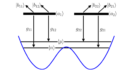
Figure 2: (Color online) Model for condensation in a double-well potential, in which two orbitals, extended across the well due to tunneling, are pumped by independent reservoirs localized on the left and right. The occupations of the two delocalized orbitals are denoted $n$ and $p$.

As shown in Fig. 2, we consider a situation in which the two lowest orbitals of a double-well potential are being pumped by two reservoirs, one for each of the wells. We begin with a tight-binding model for the low-energy orbitals, with Hamiltonian

$$H_{LR}=\Delta\epsilon(a_{R}^{\dagger}a_{R}-a_{L}^{\dagger}a_{L})-t(a_{R}^{\dagger}a_{L}+a_{L}^{\dagger}a_{R})+H_{LR(NL)},$$ (54)

where $a_{L}$ and $a_{R}$ are the annihilation operators for polaritons in orbitals localized on the left and right. $\Delta\epsilon$ is the detuning, i.e., the energy difference between these orbitals, and $t$ is the tunneling matrix element. We use

$$H_{LR(NL)}=g[(a_{L}^{\dagger}a_{L})^{2}+(a_{R}^{\dagger}a_{R})^{2}],$$ (55)

to model the repulsive interactions within the condensates. Note that we have assumed, for simplicity, that the direct overlap of the localized orbitals is small, and hence neglected any off-diagonal interaction terms in the localized basis. We have also assumed that the localized orbitals are the same size, so that the interaction strength is the same for each.

The first step is to diagonalize the quadratic part of the Hamiltonian, and transform to the basis of single-particle eigenstates. This is accomplished by the standard transformation

$$\begin{pmatrix}a_{L}\\ a_{R}\end{pmatrix}=\begin{pmatrix}\cos(\theta)&-\sin(\theta)\\ \sin(\theta)&\cos(\theta)\end{pmatrix}\begin{pmatrix}a_{1}\\ a_{2}\end{pmatrix},$$ (56)

with $\tan(2\theta)=t/\Delta\epsilon$, which gives

$$H=\Delta E(a_{2}^{\dagger}a_{2}-a_{1}^{\dagger}a_{1})+H_{(NL)},$$ (57)

where $\Delta E=\sqrt{\Delta\epsilon^{2}+t^{2}}$. At zero detuning, $a_{1}$ and $a_{2}$ annihilate particles in symmetric or antisymmetric orbitals extended over the double well.

The normalized transition strengths between the condensates and the reservoirs $\alpha_{ij}$, defined in Eq. (16), follow from Eq. (56). Since the two reservoirs are equivalent, these ratios are just the fraction of the density in each orbital that lies over each reservoir, i.e., on the left or the right of the junction:

$$\alpha_{11}=\alpha_{22}=\cos^{2}(\theta)=\tfrac{1}{2}+\frac{\Delta\epsilon}{2\sqrt{\Delta\epsilon^{2}+t^{2}}}$$

$$\alpha_{12}=\alpha_{21}=\sin^{2}(\theta)=\tfrac{1}{2}-\frac{\Delta\epsilon}{2\sqrt{\Delta\epsilon^{2}+t^{2}}}.$$ (58)

Finally, we need the coefficients in the interaction Hamiltonian, Eq. (23). Writing Eq. (55) in the $a_{1,2}$ basis, and comparing with Eq. (23), gives

$$\kappa=g[\sin^{4}(\theta)+\cos^{4}(\theta)]=\frac{g}{2}\left(1+\frac{\Delta\epsilon^{2}}{\Delta\epsilon^{2}+t^{2}}\right),$$

$$\eta=8g\sin^{2}(\theta)\cos^{2}(\theta)=\frac{2g\,t^{2}}{\Delta\epsilon^{2}+t^{2}}.$$ (59)

The transformation of Eq. (55) to the single-particle eigenbasis also generates the interaction terms

$$\begin{split}\frac{g}{2}\Big{[}&\sin^{2}(2\theta)a_{1}^{\dagger}a_{1}^{\dagger}a_{2}a_{2}\\ &+\sin(4\theta)(a_{2}^{\dagger}a_{2}^{\dagger}a_{2}a_{1}-a_{1}^{\dagger}a_{1}^{\dagger}a_{1}a_{2})\Big{]}+\mathrm{h.c.},\end{split}$$ (60)

which describe the scattering of particles between different orbitals. As discussed in Sec. III.1, we treat the quasilinear regime, where the strength of these terms is smaller than the level spacing of the non-interacting Hamiltonian, so that they are a small perturbation. For the two-well problem the condition for this approximation to be valid is parametrically

$$\Delta E=\sqrt{\Delta\epsilon^{2}+t^{2}}\gtrsim gn.$$ (61)

Here we neglect numerical factors, which are of order 1 in typical geometries, including the trigonometric functions in Eq. (60). When Eq. (60) is satisfied the density generically undergoes sinusoidal oscillations, while the relative phase between the condensates can either oscillate or wind (linear “Rabi” oscillations and linear “Josephson” oscillations, respectivelyAbbarchi et al. (2013)). For the special case $\Delta\epsilon=0$ Eq. (60) is the criterion defining the Rabi regime as given by Leggett.Leggett (2001) It excludes any situation in which the density imbalance is determined by interactions, rather than by the pumping alone. We discuss this further in Appendix C.

IV.1 Population distribution

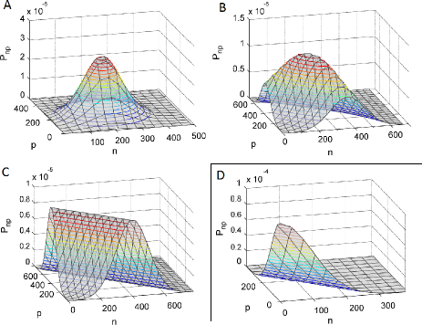
Figure 3: (Color online) Probability distribution of the populations $n,p$ of the two orbitals of a double-well potential, pumped by independent reservoirs for each well. Panels A–C: Results above the mean-field threshold, with $n_{c}=5200,\,n_{s}=5000$, and the reservoir to mode couplings varying as $\alpha_{11}=\alpha_{22}=1$ (A), 0.66 (B), 0.5 (C), and $\alpha_{12}=\alpha_{21}=0$ (A), 0.33 (B), 0.5 (C). This corresponds to decreasing the detuning or increasing the tunneling, so that the eigenstates evolve from localized orbitals of each well to delocalized, symmetric-antisymmetric superpositions. A soft mode develops along the $n+p$ direction as the tunneling is increased and the modes become pumped indiscriminately by the two reservoirs. Panel D: distribution at the mean-field threshold, $n_{c}=n_{s}=5000$, for $\alpha_{11}=\alpha_{22}=1$, $\alpha_{12}=\alpha_{21}=0$.

In Fig. 3 we show the population distribution among the orbitals of the double well, obtained by using Eq. (58) in Eq. (II.2). We take $n_{s}$ $=$ $5000$, which is physically reasonableWhittaker and Eastham (2009) while also in a regime which is convenient to contrast the approaches presented in Sec. III. We show results when the pump parameter $n_{c}$ is both at the mean-field threshold ($n_{c}$ $=$ $n_{s}$; panel D), and above threshold ($n_{c}$ $=$ $5200$; panels A–C). Above threshold we show how the distribution varies with tunneling or detuning, giving results for three steps from vanishing tunneling ($t/\Delta\epsilon$ $=$ $0$, panel A) to vanishing detuning ($t/\Delta\epsilon$ $\to$ $\infty$, panel C). For vanishing tunneling the orbitals are localized in the left and right well, and the double-well system comprises two independent condensates. The population distribution above threshold is then a symmetrical two-dimensional Gaussian ($P_{np}$ $=$ $P_{n}P_{p}$). However, as we increase the tunneling, or decrease the detuning, the orbitals become more delocalized between the left and right, and hence receive pumping from both reservoirs. The distribution broadens along the direction $n$ $=$ $p$, until at resonance the distribution is a flat ridge along this direction ($P_{np}$ $=$ $P_{[n+p]}|_{n,p\geq 0}$). This is because the pumping is related to the density profile of the condensate orbitals, which is identical for the two modes at resonance. Thus, the pumping does not distinguish between the two orbitals, fixing only the total density $n$ $+$ $p$, and leaving the difference $n$ $-$ $p$ undetermined, within $n,p$ $\geq$ $0$. In other words, there is a soft mode describing density fluctuations between the two condensate orbitals. The effects of the soft mode are limited by the cut-off at $n$ $=$ $p$ $=$ $0$, so that the population distribution in this case is not a Gaussian. Furthermore, there are large fluctuations in the populations, which persist even far above threshold, $n_{c}$ $\gg$ $n_{s}$. We note that $\Delta\epsilon$ $=$ $0$ corresponds to a nonequilibrium phase boundary at the mean-field (rate-equation) level,Eastham (2008) separating the single-mode and two-mode steady-states. The large fluctuations found here correspond to critical fluctuations near this phase transition, associated with the finite size of the condensate.Eastham and Littlewood (2006)

IV.2 First-order coherence functions

In Fig. 4 we show the first-order coherence functions for the light emitted from one mode of a double-well. The left panel (A) shows the results obtained by direct numerical solution of Eq. (III.2), while the right panel (B) shows those of the Fokker-Planck and static-limit approaches. We again show results at the mean-field threshold, and slightly above it, and for both vanishing tunneling and vanishing detuning.

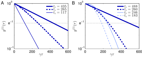
Figure 4: (Color online) First-order coherence functions for the emission from one mode of a double-well potential, with $g=4\times 10^{-5}\gamma$ and $n_{s}=5000$. Solid curves show results for vanishing interwell tunneling ($t/\Delta\epsilon=0$), and dotted curves for vanishing detuning ($t/\Delta\epsilon\to\infty$). Left panel (A): Numerical results with $n_{c}=5000$ (thin line) and $5200$ (thick lines). Right panel (B): Static limit approximation (light blue) and Fokker-Planck approximation (dark blue), for $n_{c}=5200$. The insets give the corresponding coherence times in units of $1/\gamma$.

For all parameters shown, the numerical solution gives an exponential decay of the first-order coherence, i.e., a Lorentzian emission line. This is the same form found previously for a single mode,Whittaker and Eastham (2009) and corresponds to interaction broadening in the motional narrowing regime.Kubo (1954); Hamm (2005) That the result is due to interaction effects is shown by the observation that the computed coherence times are similar to those obtained from the static limit calculation. The static limit, however, is deprived of the motional narrowing effectKubo (1954); Whittaker and Eastham (2009) and shows its hallmark Gaussian decay for the first-order coherence. For larger polariton-polariton interaction strengths or broader population distributions, the static regime dominates, and the numerical solution and the static limit result coincide.

The full dependence of the coherence time, as predicted by the static limit and Fokker-Planck approaches, is shown in Fig. 5. The coherence time decreases, so the linewidth broadens, as we go from localized independent condensates (zero tunneling) to delocalized coupled condensates (zero detuning). This is because the broadening reflects the population fluctuations, which cause energetic fluctuations via the interaction, and the population fluctuations are largest for the delocalized case (see Fig. 3). This effect is counterbalanced by the changes in interaction strengths, $\kappa,\eta$, with detuning Eqs. (59). Even though in the distributed case the condensates overlap with one another and the average interaction strength is stronger than in the independent case ($\frac{\kappa}{g},\frac{\eta}{g}$ $=$ $0.5,2$ vs $1,0$), the populations are anticorrelated between the modes. The resulting energy fluctuations, therefore, to some extent cancel. To separate this effect we show the coherence time obtained in the static limit taking $\kappa$ $=$ $g$ and $\eta$ $=$ $0$ (panel A, light blue). This produces a basic step-like form of the coherence time.

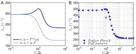
Figure 5: (Color online) Dependence of the coherence time (in units of $1/\gamma$) on the ratio of tunneling to detuning, $t/\Delta\epsilon$, for $n_{c}=5200$ and $n_{s}=5000$. Left panel (A): Static limit approximation, with $\kappa,\eta$ given by Eq. (59) (dark blue), and with $\kappa,\eta=g,0$ (light blue). Right panel (B): Fokker-Planck approximation and full numerical solution.

When the dependence of the interaction strengths on detuning is included two additional features are noticeable in the static limit (panel A, dark blue): a non-monotonic dependence of the coherence time, and an overall increase of the coherence time at $t/\Delta\epsilon\approx 1$. The inter-condensate interaction is responsible for these effects. The fluctuations in the populations of the modes are anticorrelated at strong tunneling, because the total occupation, $n\!+\!p$, is fixed by the pumping. Since an increase in the occupation of one mode tends to be accompanied by a decrease in the occupation of the other, the energy shifts generated by the interaction within the modes are partially canceled by those between the modes. In this way the inter- and intra-condensate interactions act in conjunction to preserve and even increase coherence. In the motional narrowing regime, as shown in the Fokker-Planck and full numerical solutions (panel B), fluctuations acquire a more isotropic nature and this effect vanishes.

Finally, we see from Figs. 4 and 5 that the Fokker-Planck approximation is in good agreement with the full numerical calculation. We note that, for strong tunneling, the Fokker-Planck approximation indicates a Gaussian behavior for the first-order coherence function, similar to that seen in the static limit. We suggest this is an effect of the soft density mode. In the Fokker-Planck approach the drift coefficients are approximated as linear functions of the populations, giving a divergent relaxation time for fluctuations of $n$ $-$ $p$. Thus, the soft mode has no dynamics at the level of the linearized theory, and we obtain behavior similar to that of the static limit. In the full theory, nonlinear effects are in place and this slow dynamics is suppressed.

IV.3 Coherence of Josephson oscillations

In Fig. 6 we show the decay of the second-order correlation function $g^{J}(\tau)$, describing the dephasing of the intensity oscillations, obtained from both the numerical solution of Eq. (III.5), and from the static limit result, Eq. (53). Comparing with Fig. 4 we see that, when the interwell tunneling vanishes, the decay time for $g^{J}(\tau)$ is half that of the first-order coherence function $g^{(1)}(\tau)$, for the exponential decays obtained from the numerical solution. For the Gaussian decays, obtained in the static limit, the corresponding factor is $1/\sqrt{2}$. This is as expected, since for independent emitters $g^{J}$ factorizes, $\langle a_{1}^{\dagger}(\tau)a_{2}(\tau)a_{2}^{\dagger}a_{1}\rangle=\langle a_{1}^{\dagger}(\tau)a_{1}\rangle\langle a_{2}(\tau)a_{2}^{\dagger}\rangle$. Such a factorization does not, in general, apply in the case where the modes interact, and indeed we see that for the numerical solution shown the decay of $g^{J}$ occurs faster than would be expected from independent emitters. This reflects the correlations between the modes, which can be caused both by the Hamiltonian and the dissipative interactions through the common reservoirs.

We make two additional comments regarding the relation between $g^{J}$ and $g^{(1)}$. First, for all the parameters shown the ratio of the coherence times in the static limit appears to be $1/\sqrt{2}$, even when the intermode interactions are present. One can readily check, however, that $g^{J}$ does not factorize in this case, although this is not apparent from these coherence times. Second, we note that for independent emitters $g^{J}$ strictly factorizes into a product of $g^{(1)}(\tau)$ and an antinormal ordered correlation function $\langle a(\tau)a^{\dagger}\rangle$; the latter corresponds to an absorption spectrum. The decay times for these two types of correlators can, in principle, differ in an interacting system, where the dynamics after adding a particle is not equivalent to that after removing one. This difference is negligible here, however, since the range of occupation numbers in the steady-state density matrix is much larger than 1.

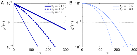
Figure 6: (Color online) Decay of the second-order cross-correlation function $g^{J}(\tau)$, describing the dephasing of intensity (Josephson) oscillations in the strong-trapping (Rabi) regime of a double-well potential. Corresponding results for the first-order coherence function are shown in Fig. 4. Solid curves: Vanishing interwell tunneling. Dotted curves: vanishing detuning. Left panel (A): Numerical results with $n_{c}=5000$ (thin line), $5200$ (thick lines). Right panel (B): Static limit approximation for $n_{c}=5200$.

V Discussion

Although we have focused on the specific example of condensation in a double-well potential, our theory can be applied to a range of many-condensate systems now being considered,Lagoudakis et al. (2010); Masumoto et al. (2012); Tosi et al. (2012); Galbiati et al. (2012) once they have been decomposed into the appropriate single-particle orbitals. Each such orbital comprises a possible condensate mode in our theory, with gain and loss characterized by a few phenomenological parameters. In general the decoherence of the condensate depends on the structure of the single particle orbitals, so our theory allows for the study and optimization of coherence properties of polariton condensates across the geometries now being developed, including wires, photonic molecules, and photonic crystals. More speculatively, it could provide a basis for studying glasslike statesJanot et al. (2013); Malpuech et al. (2007) and spontaneous vortex lattices,Keeling and Berloff (2008) beyond the mean-field level, and also for treatments of polariton dynamics in the quantum correlated regime.Carusotto and Ciuti (2013)

One notable feature in experiments is the presence of a large repulsive interaction with the reservoir excitons.Tosi et al. (2012); Wouters et al. (2008) We have omitted this from our discussion, because it can be included on average as an effective potential, and hence a redefinition of the orbitals. Fluctuations in the reservoir occupation can broaden the emission line, i.e., lead to decoherence of the condensate, but this is negligible compared with the intrinsic linewidth provided pump laser noise is small and fast.Love et al. (2008); Poddubny et al. (2013) Schwendimann, Quattropani, and Sarchi have recently discussed an additional decoherence mechanism for polariton condensates, involving parametric scattering processes, and predicted its effects for a single-mode condensate.Schwendimann et al. (2010) It would be interesting to extend our theory to include this process, and hence assess its impact in multimode condensates.

We have presented the theory without explicit consideration of the polarization of the polaritons.Shelykh et al. (2010) In incoherently pumped systems, the effects of this additional degree of freedom have been explored in both experiment and theory; the key result is that the condensate shows a high degree of linear polarization, in a direction pinned to the crystal axes.Kasprzak et al. (2007); Klopotowski et al. (2006); Shelykh et al. (2006); Laussy et al. (2006) In principle our theory allows the treatment of polarization, beyond the mean-field (Gross-Pitaevskii) level, in two regimes.

Polarization can be included relatively straightforwardly within our theory, when the polarization splitting of the single-particle orbitals is negligible. In CdTe microcavities extrinsic effects, probably strain, do induce such splittings, but they are typically small, $\Omega_{ph}\sim\mu\mathrm{eV}$.Krizhanovskii et al. (2009) Neglecting this scale we may take each spatial orbital in our theory to comprise two degenerate circularly polarized orbitals, for polaritons with $J_{z}=\pm 1$. Within each such orbital the interaction Hamiltonian isShelykh et al. (2010)

$$c_{1}(n_{+}^{2}+n_{-}^{2})+c_{2}n_{+}n_{-},$$ (62)

where $n_{+(-)}$ are the numbers of polaritons of each circular polarization. Since this is of the same form as Eq. (23), i.e., diagonal in Fock space, in the circular basis, the form of our theory is unaffected, although the number of modes is, in general, doubled. (However, $|c_{1}|\gg|c_{2}|\approx 0$,Magnusson et al. (2010) so that if the polarizations have independent reservoirs they completely decouple to a good approximation, and the number of modes is effectively unchanged.)

Although a full analysis of this case is beyond the scope of this paper, we can anticipate some results and ramifications. Each spatial mode will give rise to two coherent circularly polarized emitters, each with a linewidth determined by the co-polarized interactions (the broadening due to the cross-polarized interactions will be smaller, because $|c_{2}|\ll|c_{1}|$). The relative occupation of the two circular polarizations will depend on the scattering processes. In incoherently pumped systems, a reasonable assumptionShelykh et al. (2010); Martín et al. (2002) is that relaxation processes provide for the gain and nonlinear gain to be equivalent for the two circular polarizations, so that the resulting occupations are identical, and the emission for each spatial mode is then linearly polarized on average. This argument is very similar to those previously used to explain the linear polarization of polariton condensates:Shelykh et al. (2006); Laussy et al. (2006) the choice of the circular basis arises because this diagonalizes the interaction Hamiltonian, and the reasonable assumption of an equal population of such eigenstates (which gives the minimum energy in equilibrium) is then a linear polarization. If the two circular polarizations are truly degenerate, $\Omega_{ph}=0$, then the direction of linear polarization would fluctuate from shot to shot, but it can be locked by a non-zero $\Omega_{ph}$.Read et al. (2010) For a single spatial mode Laussy et al.Laussy et al. (2006) have gone beyond mean-field theory to predict the decay time of the polarization, considering the Hamiltonian evolution alone, i.e., in the static limit (c.f. Sec III.4); we expect motional narrowing to extend this decay time in general.

The approach in terms of circularly polarized basis states breaks down when, sufficiently far above threshold, the linewidths become smaller than $\Omega_{ph}$, which is no longer a small energy scale. In this regime one should take the (typically) linearly polarized eigenstates of the single-particle Hamiltonian as the starting point. However, transforming the interaction, Eq. (62), to this basis leads to polarization-flip scattering terms, such as $a_{x}^{\dagger}a_{x}^{\dagger}a_{y}a_{y}$. This is of the form of Eq. (24), but unfortunately since $\Omega_{ph}$ is usually small compared with the interaction energy it cannot be similarly neglected. Thus this regime cannot be fully treated within the framework of our theory, unless it is extended to include non-conserving scattering processes, i.e., spin-flip terms. An exception is when only one of the two orthogonal polarizations is populated, which can indeed occur,Krizhanovskii et al. (2009) so that the unoccupied orthogonally polarized mode may be omitted completely from the description.

VI Conclusion

In summary, we have developed a model for the nonequilibrium dynamics of polaritons in an incoherently pumped microcavity, incorporating gain due to scattering from multiple reservoirs, and resonant polariton-polariton interactions. In contrast to previous works addressing condensates formed with a single macroscopically-occupied orbital, our theory applies when several such states coexist, i.e., to multimode polariton condensates. We have used it to predict the quantum statistics, revealed for example via the linewidths, and shown how these quantities are affected by interactions between the condensates. We predict that the populations of the modes can be anticorrelated due to their coupling to a common reservoir, leading to a narrowing of the emission lines and a prolongation of the coherence time. We have also demonstrated theoretically a dephasing mechanism for intensity oscillations, and shown that, for realistic parameters, their coherence decay provides a useful probe of correlation effects.

An important theoretical extension of our work would be to include the nonresonant interaction terms between the modes, in particular terms such as $a_{1}^{\dagger}a_{1}^{\dagger}a_{2}a_{2}$, which become significant beyond the strong-trapping regime. This would also allow us to include spin-flip and polarization dependent mechanisms.Glazov et al. (2013); Magnusson et al. (2010) In Fock space, the Liouville evolution of these terms generates a recursive dependence on all the elements within density matrix. This contrasts with having to solve for the diagonal elements in the case of steady-state population distribution or the one off-diagonal terms for linewidth and Josephson coherence function. We suggest that these interactions could be included by generalizing the Fokker-Planck approach to apply to the full density operator, rather than the distributions $u$ or $P$, i.e., by assuming $\rho_{mnpq}$ is smooth, so that Eq. (1) becomes a partial differential equation. Such an approach would be similar in spirit to those based on the Wigner representation for $\rho$, as discussed by Wouters and SavonaWouters and Savona (2009) among others. It could also be done without consideration of the classical limit of quantum electrodynamics and make use of the Mellin transform in relation to fractional calculus,Sabatier et al. (2007); Das (2011) in contrast to the double-sided Laplace transform which led to Eq. (46). More numerically driven, the cumulant expansion technique used in Ref. Magnusson et al., 2010 may also lead to a way to deal with these terms. The non resonant interaction terms lead to the Bogoliubov spectrum for a homogeneous single-mode condensate, and hence are implicated in superfluidity, while at the semiclassical level they cause nonlinear mixing and synchronization in the multimode case.Eastham (2008) The suggested generalization of our theory would allow the impact of quantum and nonequilibrium fluctuations on such phenomena to be explored, in complex geometries where many condensates coexist. Josephson phenomena which occur outside the strong-trapping regime are also accessible once these terms are included.

Appendix A Derivation of the Effective Pumping Rate

To derive an effective pumping rate, $r$, starting from the replenishing rate, $\lambda_{a}$, of reservoir level $|a\rangle$, we combine the system to a generic level, $\Phi=\rho^{\phi\phi}|\phi\rangle\!\langle\phi|$, giving $\rho\otimes\Phi$. The evolution of the coupled system, projected onto $|\phi\rangle$, provides the rate equation,

$$0=-\lambda_{a}\rho_{nmpq}^{\phi\phi}+\gamma_{r}(\rho_{nmpq}^{aa}+\rho_{nmpq}^{b_{1}b_{1}}+\rho_{nmpq}^{b_{2}b_{2}}),$$ (63)

which we use in conjunction with the trace over all levels, $\mathrm{Tr}_{a,b_{i},\phi}[\rho\otimes\Phi]$,

$$\rho_{nmpq}=\rho_{nmpq}^{\phi\phi}+\rho_{nmpq}^{aa}+\rho_{nmpq}^{b_{1}b_{1}}+\rho_{nmpq}^{b_{2}b_{2}}$$ (64)

Substituting $\rho_{nmpq}-\rho_{nmpq}^{\phi\phi}$ for $\rho_{nmpq}^{aa}+\rho_{nmpq}^{b_{1}b_{1}}+\rho_{nmpq}^{b_{2}b_{2}}$, (64), into (63) gives

$$\rho_{nmpq}^{\phi\phi}=\frac{\gamma_{r}}{\lambda_{a}+\gamma_{r}}\rho_{nmpq}.$$ (65)

Hence

$$\lambda_{a}\rho_{nmpq}^{\phi\phi}=\cfrac{\lambda_{a}\gamma_{r}}{\lambda_{a}+\gamma_{r}}\rho_{nmpq}=r\rho_{nmpq},$$ (66)

and we have transformed the repopulation from level $\Phi$ into an effective pumping, with rate $r$. Additional levels could be included, but their steady-state nature allows us to recover this simpler scheme.Scully and Zubairy (1997)

Appendix B Intermediate Vector and Matrix Forms in the Simplified Pumping Model

To obtain the one reservoir, two modes dissipator (II.1), we generate three versions of these vector forms,

$$R=\begin{pmatrix}\rho_{nmpq}^{aa}\\ \rho_{nm+1pq}^{ab_{1}}\\ \rho_{n+1mpq}^{b_{1}a}\\ \rho_{nmpq+1}^{ab_{2}}\\ \rho_{nmp+1q}^{b_{2}a}\\ \rho_{n+1mpq+1}^{b_{1}b_{2}}\\ \rho_{nm+1p+1q}^{b_{2}b_{1}}\\ \rho_{n+1m+1pq}^{b_{1}b_{1}}\\ \rho_{nmp+1q+1}^{b_{2}b_{2}}\end{pmatrix},\quad A=r\begin{pmatrix}\rho_{nmpq}\\ 0\\ 0\\ 0\\ 0\\ 0\\ 0\\ 0\\ 0\end{pmatrix}.$$ (67)

We also use three instances of the following matrix form,

$$M=\begin{pmatrix}\gamma_{r}&-ig_{1}\sqrt{m+1}&ig_{1}\sqrt{n+1}&-ig_{2}\sqrt{q+1}&ig_{2}\sqrt{p+1}&0&0&0&0\\ -ig_{1}\sqrt{m+1}&\gamma_{r}&0&0&0&0&ig_{2}\sqrt{p+1}&ig_{1}\sqrt{n+1}&0\\ ig_{1}\sqrt{n+1}&0&\gamma_{r}&0&0&-ig_{2}\sqrt{q+1}&0&-ig_{1}\sqrt{m+1}&0\\ -ig_{2}\sqrt{q+1}&0&0&\gamma_{r}&0&ig_{1}\sqrt{n+1}&0&0&ig_{2}\sqrt{p+1}\\ ig_{2}\sqrt{p+1}&0&0&0&\gamma_{r}&0&-ig_{1}\sqrt{m+1}&0&-ig_{2}\sqrt{q+1}\\ 0&0&-ig_{2}\sqrt{q+1}&ig_{1}\sqrt{n+1}&0&\gamma_{r}&0&0&0\\ 0&ig_{2}\sqrt{p+1}&0&0&-ig_{1}\sqrt{m+1}&0&\gamma_{r}&0&0\\ 0&ig_{1}\sqrt{n+1}&-ig_{1}\sqrt{m+1}&0&0&0&0&\gamma_{r}&0\\ 0&0&0&ig_{2}\sqrt{p+1}&-ig_{2}\sqrt{q+1}&0&0&0&\gamma_{r}\\ \end{pmatrix}.$$ (68)

The vectors and matrices $R^{\prime},A^{\prime},M^{\prime}$ and $R^{\prime\prime},A^{\prime\prime},M^{\prime\prime}$ are obtained by shifting the indices and occupation numbers of $R,A,M$ according to $n,m\rightarrow n-\!1,m-\!1$ and $p,q\rightarrow p\!-\!1,q\!-\!1$, respectively. We use the elements $M_{21}^{-1}..M_{51}^{-1}$, $M^{\prime-1}_{21},M^{\prime-1}_{31}$ and $M^{\prime\prime-1}_{41},M^{\prime\prime-1}_{51}$ in our substitution.

Appendix C Regimes of Josephson junctions

Within the mean-field (Gross-Pitaevskii) dynamics of a Josephson junction one typically discusses several different regimes, and a range of Josephson effects within each regime. If Eq. (61) holds then the mean-field dynamics is that of two coupled harmonic oscillators, leading to our description of this regime as linear. In it one obtains sinusoidal oscillations in the density from the beating between normal modes.Javanainen (1986) Since this is also the physics of Rabi oscillations of a two-state system, the linear regime is sometimes also described as the Rabi regime. In the literature the criterion for the linear/Rabi regimeLeggett (2001); Raghavan et al. (1999); Abbarchi et al. (2013) is usually stated for the case where the detuning, $\Delta\epsilon$, is zero, or at least similar to the tunneling, $t$, and so is $t\gtrsim gn$. For $\Delta\epsilon\neq 0$ the behavior at the mean-field level can remain linear (constant blueshifts, of order $gn$, excepted) even for very small tunneling, so long as Eq. (61) is satisfied. The opposite regime, where the interactions dominate, is usually labeled as the Josephson regime, and is where macroscopic quantum self-trapping is studied.

The experiment involving continuous incoherent pumping,Lagoudakis et al. (2010) as in our theory, is generally agreed to be in the linear/Rabi regime,Lagoudakis et al. (2010); Abbarchi et al. (2013) so that we expect our theory to apply. We note, however, one potential complication. If interactions like Eq. (60) are completely neglected then there are no terms which fix the relative phase of the condensates in the two modes. Thus the phase of the Josephson oscillations would fluctuate from shot to shot of an experiment [see Eq. (49)]. The data reported in Ref. Lagoudakis et al., 2010 are, however, averaged over many repetitions and still reveal oscillations, so that a consistent phase is being established. Thus the terms in Eq. (60) do have some effect, perhaps implying some small corrections to our results.

As noted above, some other recent experiments involve coherent resonant excitation to create a transient condensate.Abbarchi et al. (2013) The linear regime discussed by these authors would correspond to Eq. (61) being satisfied, while the nonlinear regime (where macroscopic quantum self-trapping was observed) would be where it is violated; the further distinction made within the linear regime, between “Rabi” and “Josephson” oscillations, would not be relevant in terms of the applicability of our theory. It is, in any case, not directly relevant to these experiments, as they have neither a condensed steady-state nor incoherent excitation.

References

- Hopfield (1958) J. J. Hopfield, Phys. Rev. 112, 1555 (1958).
- Weisbuch et al. (1992) C. Weisbuch, M. Nishioka, A. Ishikawa, and Y. Arakawa, Phys. Rev. Lett. 69, 3314 (1992).
- Dang et al. (1998) L. S. Dang, D. Heger, R. André, F. Boeuf, and R. Romestain, Phys. Rev. Lett. 81, 3920 (1998).
- Kasprzak et al. (2006) J. Kasprzak, M. Richard, S. Kundermann, A. Baas, P. Jeambrun, J. M. J. Keeling, F. M. Marchetti, M. H. Szymanska, R. Andre, J. L. Staehli, V. Savona, P. B. Littlewood, B. Deveaud, and L. S. Dang, Nature 443, 409 (2006).
- Love et al. (2008) A. P. D. Love, D. N. Krizhanovskii, D. M. Whittaker, R. Bouchekioua, D. Sanvitto, S. A. Rizeiqi, R. Bradley, M. S. Skolnick, P. R. Eastham, R. André, and L. S. Dang, Phys. Rev. Lett. 101, 067404 (2008).
- Assmann et al. (2011) M. Assmann, J.-S. Tempel, F. Veit, M. Bayer, A. Rahimi-Iman, A. Loeffler, S. Hoefling, S. Reitzenstein, L. Worschech, and A. Forchel, Proc. Natl. Acad. Sci. USA 108, 1804 (2011).
- Pitaevskii and Stringari (2003) L. Pitaevskii and S. Stringari, Bose-Einstein Condensation, International Series of Monographs on Physics, Vol. 116 (Oxford University Press, London, 2003).
- Tosi et al. (2012) G. Tosi, G. Christmann, N. G. Berloff, P. Tsotsis, T. Gao, Z. Hatzopoulos, P. G. Savvidis, and J. J. Baumberg, Nat. Phys. 8, 190 (2012).
- Galbiati et al. (2012) M. Galbiati, L. Ferrier, D. D. Solnyshkov, D. Tanese, E. Wertz, A. Amo, M. Abbarchi, P. Senellart, I. Sagnes, A. Lemaître, E. Galopin, G. Malpuech, and J. Bloch, Phys. Rev. Lett. 108, 126403 (2012).
- Lagoudakis et al. (2010) K. G. Lagoudakis, B. Pietka, M. Wouters, R. André, and B. Deveaud-Plédran, Phys. Rev. Lett. 105, 120403 (2010).
- Abbarchi et al. (2013) M. Abbarchi, A. Amo, V. G. Sala, D. D. Solnyshkov, H. Flayac, L. Ferrier, I. Sagnes, E. Galopin, A. Lemaître, G. Malpuech, and J. Bloch, Nat. Phys. 9, 275 (2013).
- Lai et al. (2007) C. W. Lai, N. Y. Kim, S. Utsunomiya, G. Roumpos, H. Deng, M. D. Fraser, T. Byrnes, P. Recher, N. Kumada, T. Fujisawa, and Y. Yamamoto, Nature 450, 529 (2007).
- Masumoto et al. (2012) N. Masumoto, N. Y. Kim, T. Byrnes, K. Kusudo, A. Löffler, S. Höfling, A. Forchel, and Y. Yamamoto, New J. Phys. 14, 065002 (2012).
- Langbein et al. (1999) W. Langbein, J. M. Hvam, and R. Zimmermann, Phys. Rev. Lett. 82, 1040 (1999).
- Wouters and Carusotto (2007) M. Wouters and I. Carusotto, Phys. Rev. Lett. 99, 140402 (2007).
- Keeling and Berloff (2008) J. Keeling and N. G. Berloff, Phys. Rev. Lett. 100, 250401 (2008).
- Eastham (2008) P. R. Eastham, Phys. Rev. B 78, 035319 (2008).
- Rodrigues et al. (2012) A. S. Rodrigues, P. G. Kevrekidis, J. Cuevas, R. Carretero-Gonzalez, and D. J. Frantzeskakis, arXiv:1205.6262 (2012).
- Szymańska et al. (2007) M. H. Szymańska, J. Keeling, and P. B. Littlewood, Phys. Rev. B 75, 195331 (2007).
- Tassone and Yamamoto (2000) F. Tassone and Y. Yamamoto, Phys. Rev. A 62, 063809 (2000).
- Haug et al. (2012) H. Haug, T. D. Doan, H. T. Cao, and D. B. T. Thoai, Phys. Rev. B 85, 205310 (2012).
- Wouters and Savona (2009) M. Wouters and V. Savona, Phys. Rev. B 79, 165302 (2009).
- Whittaker and Eastham (2009) D. M. Whittaker and P. R. Eastham, EPL 87, 27002 (2009).
- Schwendimann et al. (2010) P. Schwendimann, A. Quattropani, and D. Sarchi, Phys. Rev. B 82, 205329 (2010).
- Porras and Tejedor (2003) D. Porras and C. Tejedor, Phys. Rev. B 67, 161310 (2003).
- Laussy et al. (2004) F. P. Laussy, G. Malpuech, A. Kavokin, and P. Bigenwald, Phys. Rev. Lett. 93, 016402 (2004).
- Verger et al. (2006) A. Verger, C. Ciuti, and I. Carusotto, Phys. Rev. B 73, 193306 (2006).
- Schwendimann and Quattropani (2008) P. Schwendimann and A. Quattropani, Phys. Rev. B 77, 085317 (2008).
- Savenko et al. (2011) I. G. Savenko, E. B. Magnusson, and I. A. Shelykh, Phys. Rev. B 83, 165316 (2011).
- Wouters (2008) M. Wouters, Phys. Rev. B 77, 121302 (2008).
- Singh and Zubairy (1980) S. Singh and M. S. Zubairy, Phys. Rev. A 21, 281 (1980).
- Kampen (2007) N. V. Kampen, Stochastic Processes in Physics and Chemistry, 3rd ed. (North Holland, Amsterdam, 2007).
- Scully and Zubairy (1997) M. O. Scully and M. S. Zubairy, Quantum Optics (Cambridge University Press, London, 1997).
- Aleiner et al. (2012) I. L. Aleiner, B. L. Altshuler, and Y. G. Rubo, Phys. Rev. B 85, 121301 (2012).
- Deng et al. (2010) H. Deng, H. Haug, and Y. Yamamoto, Rev. Mod. Phys. 82, 1489 (2010).
- Wertz et al. (2010) E. Wertz, L. Ferrier, D. Solnyshkov, R. Johne, D. Sanvitto, A. Lemaître, I. Sagnes, R. Grousson, A. V. Kavokin, P. Senellart, G. Malpuech, and J. Bloch, Nat. Phys. 6, 860 (2010).
- Ferrier et al. (2011) L. Ferrier, E. Wertz, R. Johne, D. D. Solnyshkov, P. Senellart, I. Sagnes, A. Lemaître, G. Malpuech, and J. Bloch, Phys. Rev. Lett. 106, 126401 (2011).
- Carmichael and Walls (1974) H. J. Carmichael and D. F. Walls, Phys. Rev. A 9, 2686 (1974).
- (39) This can be seen by setting and varying . It is also pointed out in Ref. \rev@citealpnumSinghZubairy1980. In this context it may be helpful to define normalized quantities in terms of the coupling strength to one mode, rather than the total coupling, e.g., .
- Racine (2013) D. Racine, Quantum Theory of Multimode Exciton-polariton Bose-Einstein Condensation, Ph.D. thesis, Trinity College Dublin (2013).
- Rochat et al. (2000) G. Rochat, C. Ciuti, V. Savona, C. Piermarocchi, A. Quattropani, and P. Schwendimann, Phys. Rev. B 61, 13856 (2000).
- Loudon (2000) R. Loudon, “The quantum theory of light,” (Oxford University Press, London, 2000) p. 102, 3rd ed.
- Swain (1981) S. Swain, J. Phys. A: Math. Gen. 14, 2577 (1981).
- Ford and O’Connell (1996) G. W. Ford and R. F. O’Connell, Phys. Rev. Lett. 77, 798 (1996).
- Hamm (2005) P. Hamm, “Principles of nonlinear spectroscopy: a practical approach,” Lectures of the Virtual European University on Lasers (2005), (unpublished).
- Kubo (1954) R. Kubo, J. Phys. Soc. Jpn. 9, 935 (1954).
- Leggett (2001) A. J. Leggett, Rev. Mod. Phys. 73, 307 (2001).
- Raftery et al. (2013) J. Raftery, D. Sadri, S. Schmidt, H. E. Türeci, and A. A. Houck, arXiv:1312.2963 (2013).
- Sarchi et al. (2008) D. Sarchi, I. Carusotto, M. Wouters, and V. Savona, Phys. Rev. B 77, 125324 (2008).
- Magnusson et al. (2010) E. B. Magnusson, H. Flayac, G. Malpuech, and I. A. Shelykh, Phys. Rev. B 82, 195312 (2010).
- Read et al. (2010) D. Read, Y. G. Rubo, and A. V. Kavokin, Phys. Rev. B 81, 235315 (2010).
- Eastham and Littlewood (2006) P. R. Eastham and P. B. Littlewood, Phys. Rev. B 73, 085306 (2006).
- Janot et al. (2013) A. Janot, T. Hyart, P. R. Eastham, and B. Rosenow, Phys. Rev. Lett. 111, 230403 (2013).
- Malpuech et al. (2007) G. Malpuech, D. D. Solnyshkov, H. Ouerdane, M. M. Glazov, and I. Shelykh, Phys. Rev. Lett. 98, 206402 (2007).
- Carusotto and Ciuti (2013) I. Carusotto and C. Ciuti, Rev. Mod. Phys. 85, 299 (2013).
- Wouters et al. (2008) M. Wouters, I. Carusotto, and C. Ciuti, Phys. Rev. B 77, 115340 (2008).
- Poddubny et al. (2013) A. Poddubny, M. Glazov, and A. N.S., New J. Phys. 15, 025016 (2013).
- Shelykh et al. (2010) I. A. Shelykh, A. V. Kavokin, Y. Rubo, T. Liew, and G. Malpuech, Semicond. Sci. Technol. 25, 013001 (2010).
- Kasprzak et al. (2007) J. Kasprzak, R. André, L. S. Dang, I. A. Shelykh, A. V. Kavokin, Y. G. Rubo, K. V. Kavokin, and G. Malpuech, Phys. Rev. B 75, 045326 (2007).
- Klopotowski et al. (2006) L. Klopotowski, M. Martin, A. Amo, L. Vina, I. Shelykh, M. Glazov, G. Malpuech, A. Kavokin, and R. André, Solid State Comm. 139, 511 (2006).
- Shelykh et al. (2006) I. A. Shelykh, Y. G. Rubo, G. Malpuech, D. D. Solnyshkov, and A. Kavokin, Phys. Rev. Lett. 97, 066402 (2006).
- Laussy et al. (2006) F. P. Laussy, I. A. Shelykh, G. Malpuech, and A. Kavokin, Phys. Rev. B 73, 035315 (2006).
- Krizhanovskii et al. (2009) D. N. Krizhanovskii, K. G. Lagoudakis, M. Wouters, B. Pietka, R. A. Bradley, K. Guda, D. M. Whittaker, M. S. Skolnick, B. Deveaud-Plédran, M. Richard, R. André, and L. S. Dang, Phys. Rev. B 80, 045317 (2009).
- Martín et al. (2002) M. D. Martín, G. Aichmayr, L. Viña, and R. André, Phys. Rev. Lett. 89, 077402 (2002).
- Glazov et al. (2013) M. M. Glazov, M. A. Semina, E. Y. Sherman, and A. V. Kavokin, Phys. Rev. B 88, 041309 (2013).
- Sabatier et al. (2007) J. Sabatier, O. Agrawal, and J. T. Machado, Advances in Fractional Calculus: Theoretical Developments and Applications in Physics and Engineering (Springer, Berlin, 2007).
- Das (2011) S. Das, Functional Fractional Calculus (Springer, Berlin, 2011).
- Javanainen (1986) J. Javanainen, Phys. Rev. Lett. 57, 3164 (1986).
- Raghavan et al. (1999) S. Raghavan, A. Smerzi, S. Fantoni, and S. R. Shenoy, Phys. Rev. A 59, 620 (1999).