Separation of particles leading either to decay and unlimited growth of energy in a driven stadium-like billiard

Abstract

A competition between decay and growth of energy in a time-dependent stadium billiard is discussed giving emphasis in the decay of energy mechanism. A critical resonance velocity is identified for causing of separation between ensembles of high and low energy and a statistical investigation is made using ensembles of initial conditions both above and below the resonance velocity. For high initial velocity, Fermi acceleration is inherent in the system. However for low initial velocity, the resonance allies with stickiness hold the particles in a regular or quasi-regular regime near the fixed points, preventing them from exhibiting Fermi acceleration. Also, a transport analysis along the velocity axis is discussed to quantify the competition of growth and decay of energy and making use distributions of histograms of frequency, and we set that the causes of the decay of energy are due to the capture of the orbits by the resonant fixed points.

1 Introduction

Modelling dynamical systems with mixed phase space has been one of the main challenges of the nonlinear statistical mechanics research field and has received especial attention in the last decades [1, 2, 3, 4]. Particularly, with the advance of fast computers the dynamics can be evolved over long time series letting several phenomena, some of them completely new to be observed. A class of dynamics of particular interest includes the Hamiltonian systems with time-dependent perturbation, for which energy varies with time. Moreover, a better understanding of the mixed dynamics in the phase space can be given, and phenomena related to them carefully characterized. The study of chaotic properties of systems can be found in many fields of physics such as fluids [5], plasmas [6, 7], nanotubes [8], complex networks [9]. Interesting applications and phenomena can be found in optics [10, 11, 12] and acoustic [13] if billiard dynamics is considered. Particularly, if the billiard boundaries are time dependent, applications in microwaves, [14, 15, 16] and quantum dots [17, 18, 19, 20] can also be found. Also, when a particle-particle iteration in billiard dynamics is considered, one could find synchronization [21, 22] and soft wall effects [23, 24].

In particular, a phenomenon which intrigues physicists in general is the unlimited energy growth of a bouncing particle with a driven boundary, a phenomenon called Fermi Acceleration (FA). It was introduced in earlier 1949 by Enrico Fermi [25] as an attempt to describe the mechanism in which particles that have their origin from cosmic rays, acquire very high energy. Nowadays his idea is extended to other models where average properties of the velocity or kinetic energy, for long time series, are studied. In light of this approach, a billiard type dynamics is one of the most useful systems [26] which possibly exhibits unlimited energy growth when the boundary is moving in time. The Loskutov-Ryabov-Akinshin (LRA) conjecture then gives the minimal conditions to observe such a phenomenon [27, 28]. It then claims that if a billiard has a chaotic component for the dynamics in the static boundary case, this is a sufficient condition to observe unlimited energy growth when a time-dependence on the boundary is introduced. The elliptical billiard is not described by the LRA conjecture. It is indeed integrable for the static boundary case presenting a separatrix curve separating two types of dynamical regimes: libration from rotation. The introduction of time perturbation in the boundary makes the separatrix curve to turn into a stochastic layer letting the particle suffer successive crossings from rotation to libration regions [29, 30, 31] leading to an unlimited diffusion in energy.

Recent study [32], indicates that non-linear phenomena like stickiness can act as a slowing mechanism of FA. In fact, the finite time trappings around the stability islands influence some transport properties, making the system locally less-chaotic [33]. Such influence of stickiness can be found in several models and applications on the literature [3, 4, 34, 35, 36, 37, 38]. In this paper we revisit the problem of a stadium-like billiard with oscillating circle arcs boundaries, focusing on the analysis of the mechanism that produces the decay of energy, where many low energy orbits are observed to undergo reduction of energy to an apparently stable state. We argue for existence of a critical resonance velocity where high initial velocities produce FA and low initial velocities do not experience the unlimited energy grow. Such decay is caused by influence of sticky orbits with resonance around the stability islands. It leads the chaotic orbits to suffer a temporary trapping around stability islands and then be captured by the fixed points. A statistical investigation is made in order to quantify this phenomenon. Similar approach was done previously [39, 40, 41, 42, 43, 44], but in this paper we emphasize the decay of energy and its origin in stickiness for the first time. We also discuss the statistics of transport in the velocity axis near a resonant velocity marking a separation of low energy to high energy regimes producing the decay of energy and the phenomenon of unlimited energy growth.

The paper is organized as follows. In Sec.2 we describe the dynamics of the stadium billiard and a study of its chaotic properties. Section 3 is devoted to discuss the statistical and transport analysis of the properties for both ensembles of initial conditions considering low and high energy regime. Here we also present the influence of the stickiness orbits that hold the orbits in a quasi periodic motion near the fixed points, what causes the decay of energy. Finally in Sec. 4 our final remarks and conclusions are presented.

2 Stadium billiard as model, the mapping and chaotic properties

This section is devoted to discuss the model and the equations describing the dynamics. The model consists of a classical particle (or an ensemble of non-interacting particles) moving inside a closed domain of a stadium-like shape. The stadium billiard is composed by two parallel lines connected with regions of negative curvature [45, 46]. In this paper we consider the boundary of the stadium described by three geometric control parameters, $a$ which is the width of the circle arc, $b$ indicates the depth of the curvature and $l$ is the strength of the parallel lines. Additionally, we introduce in the boundary a time dependence. The dynamics of a particle for the static version of the billiard are characterized by a constancy in the energy. However the defocusing mechanism, as proposed originally by Bunimovich [45], is responsible to generate chaotic dynamics under the condition $(4bl/a^{2})\approx(l/2R)>1$ [46, 47], where $R$ is the original radius of the Bunimovich stadium. According to the LRA conjecture, a chaotic dynamics is a sufficient condition to produce unlimited energy growth in the velocity of the particle when a time perturbation to the boundary is introduced. The unlimited diffusion in velocity generated due to collisions of a particle with a massive and time moving boundary is known in the literature as Fermi acceleration [25]. Robustness is not a characteristic of the phenomenon since inelastic collision [48, 49, 50, 51] as well as dissipation introduced by the drag-type force [52, 53] suppresses the unlimited diffusion.

As usually made in the literature, the dynamics of the particle are made by using a nonlinear mapping. We therefore take into account two distinct possibilities of the dynamics which include: (i) successive collisions and; (ii) indirect collisions. For case (i), the particle suffers successive collisions with the same focusing component while in (ii), after suffering a collision with a focusing boundary, the next collision of the particle is with the opposite focusing boundary. A schematic illustration of the both collision cases can be found in Figs. 1, 2. In between such a collision the particle can, in principle, collide many times with the two parallel borders. We have considered that the time dependence in the boundary is $R(t)=R_{0}+r\sin(wt)$, where $R_{0}=(a^{2}+4b^{2})/8b$ is the radius of the static boundary and $R_{0}\gg r$. The definition of the parameters $a$ and $b$ can be found in Fig. 2. The velocity of the boundary is obtained by

$$\dot{R}(t)={B(t)}=B_{0}\cos(wt)~{},$$ (1)

with $B_{0}=rw$ and $r$ is the amplitude of oscillation of the moving boundary while $w$ is the frequency of oscillation. In our investigation however we consider only the so called static boundary approximation (also called as a simplified version). It assumes that the boundary is fixed, which makes the time spent between collisions easy to be calculated. However the velocity after collision is calculated as if the boundary were moving. For this kind of approximation, we may find some examples of dynamical systems, whose behaviour is basically the same, considering a comparison between simplified and complete version dynamics. The Bouncer model and the Standard map are two of the examples [32, 49, 50], and the stadium billiard itself [41, 42], shows a very similar dynamics for both versions.

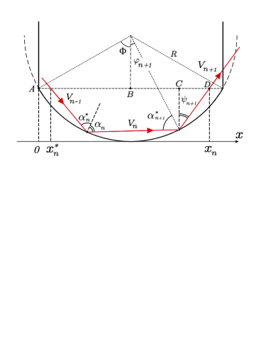
Figure 1: Sketch of the model near a focusing boundary and illustration of a typical trajectory suffering successive collisions.

The mapping is constructed for the variables $\alpha_{n}$ corresponding to the angle between the trajectory of the particle and the normal axis at the collision point, $\varphi_{n}$ is the angle measured between the normal axis at the collision points and the symmetry line of the vertical axis of the stadium, $t_{n}$ denotes the time and $V_{n}$ the outgoing speed of the particle for the nth collision. The condition to observe case (i), i.e. the successive collisions, is $|\varphi_{n+1}|<\Phi$, where $\Phi=\arcsin(a/2R_{0})$ is the angle between the vertical symmetry line and the maximum angle of the negative curvature region. A typical successive collision case is represented in Fig. 1. Using basic geometry properties we obtain

$$\left\{\begin{array}[]{ll}\alpha^{*}_{n+1}=\alpha_{n}{}\\ \varphi_{n+1}=\varphi_{n}+\pi-2\alpha_{n}~{}~{}(mod~{}2\pi){}\\ t_{n+1}=t_{n}+{2R\cos(\alpha_{n})\over V_{n}{}}\\ \end{array}\right.,$$ (2)

where the superscript $(*)$ represents the dynamical variable immediately before the collision.

Case (ii) is considered when $|\varphi_{n+1}|>\Phi$ and the particle collides with the opposite focusing component. In principle, the particle can suffer several collisions with the straight walls, so for such a type of collision, we make use of the unfolding method [26, 47] to describe the dynamics. Two auxiliary variables are then introduced, $\psi$, which is the angle between the vertical line at the collision point and the particle’s trajectory, and $x_{n}$, representing the projection over the horizontal axis. A sketch of the indirect collisions is shown in Fig. 2,

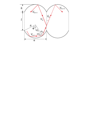
Figure 2: An illustration of the indirect collisions dynamics and its variables and parameters.

therefore leading to the following mapping

$$\left\{\begin{array}[]{ll}\psi_{n}=\alpha_{n}-\varphi_{n}~{}~{}mod(\pi/2)\\ x_{n}={R\over\cos(\psi_{n})}[\sin(\alpha_{n})+\sin(\Phi-\psi_{n})]{}\\ x_{n+1}=x_{n}+l\tan(\psi_{n})~{}~{}mod(a)\\ \alpha^{*}_{n+1}=\arcsin[\sin(\psi_{n}+\Phi)-x_{n+1}\cos(\psi_{n})/R]{}\\ \varphi_{n+1}=\psi_{n}-\alpha^{*}_{n+1}{}\\ t_{n+1}=t_{n}+{R[\cos(\varphi_{n})+\cos(\varphi_{n+1})-2\cos(\Phi)]+l\over V_{n}\cos(\psi_{n}){}}\\ \end{array}\right..$$ (3)

The expression for the velocity of the particle after collision is obtained by decomposing it into two separate components, which are

$$\left\{\begin{array}[]{ll}\vec{v}_{n}\cdot\vec{T}_{n}=v_{n}\sin(\alpha^{*}_{n}){}{}\\ \vec{v}_{n}\cdot\vec{N}_{n}=-v_{n}\cos(\alpha^{*}_{n}){}{}\\ \end{array}\right.,$$ (4)

where $\vec{T}$ and $\vec{N}$ are the tangent and normal unit vectors at the collision point. Because the collision is happening in a moving referential frame (non inertial) we have to make change of referential frames from inertial to non-inertial. The reflection law is then given by

$$\left\{\begin{array}[]{ll}\vec{V}^{\prime}_{n+1}\cdot\vec{N}_{n+1}=-\kappa\vec{V}^{\prime}_{n}\cdot\vec{N}_{n+1}{}{}\\ \vec{V}^{\prime}_{n+1}\cdot\vec{T}_{n+1}=\eta\vec{V}^{\prime}_{n}\cdot\vec{T}_{n+1}{}{}\\ \end{array}\right.,$$ (5)

where $\kappa\in[0,1]$ and $\eta\in[0,1]$ are the respective restitution coefficients for the normal and the tangent components, and the superscript ^′ resembles the non-inertial referential frame. In this paper we consider only the conservative case, therefore $\kappa=\eta=1$, although the construction of the mapping is more general.

Moving back to the inertial referential frame, the components of the velocity of the particle after collision are given by

$$\left\{\begin{array}[]{ll}\vec{V}_{n+1}\cdot\vec{N}_{n+1}=-\kappa\vec{V}_{n}\cdot\vec{N}_{n+1}+(1+\kappa)\vec{B}(t_{n+1})\cdot\vec{N}_{n+1}{}{}\\ \vec{V}_{n+1}\cdot\vec{T}_{n+1}=\eta\vec{V}_{n}\cdot\vec{T}_{n+1}+(1-\eta)\vec{B}(t_{n+1})\cdot\vec{T}_{n+1}{}{}\\ \end{array}\right.$$ (6)

Finally the velocity of the particle after collision is given by

$$\mid\vec{V}_{n+1}\mid=\sqrt{(\vec{V}_{n+1}\cdot\vec{T}_{n+1})^{2}+(\vec{V}_{n+1}\cdot\vec{N}_{n+1})^{2}}~{}.$$ (7)

The two components of the velocity can be used to obtain the angle $\alpha$, leading to

$$\alpha_{n}=\arcsin\left[{{{\mid\vec{V}_{n}\mid}\over{\mid\vec{V}_{n+1}\mid}}\sin(\alpha^{*}_{n})}\right]~{}.$$ (8)

The dynamics of the particle is then evolved by considering simultaneously equations (2), (3), (7) and (8).

3 Numerical Results and Statistical Investigation

In this section we present and discuss on how the stickiness orbits influence the dynamics. Moreover we proceed the study by doing an extensive statistical investigation in the dynamics particularly considering distributions of the angular variables along the dynamics. The novelty here is that after considering the histograms of frequency analysis for either the velocities and the polar angles for the decay of the velocity for a very long time series, we can see that the orbits after experience the stickiness influence, are captured by the fixed points, as if the dynamics was under the regime of dissipation. This makes the behaviour of the average velocity curves decays for lower energy ensembles. Also, a transport investigation along the velocity axis considering both the low and high energy regimes in order to quantify the competition between the FA and the decay of energy near the critical resonance velocity.

3.1 Resonance Velocity

Let us start discussing the resonance velocity. The phase space may be represented, according to the convenience, either using angular coordinates $\alpha_{n}$ and $\phi_{n}$, or the auxiliary variables $\psi$ and $\xi$, where $\xi=0.5+R_{0}\sin(\phi_{n+1})/a$ is the projection along the horizontal axis, and is usually normalized at $mod(1)$. The fixed points $\psi^{*}$ are deeply connected with $\alpha_{n}$ because of the axial symmetry of the billiard. There is a sequence of fixed points corresponding to orbits always within the stadium at $\phi_{n}=0$ (period-1), that intersects different multiples of the parameter $a$ in the horizontal direction, according to the unfolding method [26, 47]. They are represented in the phase space by the elliptical stability islands in Fig. 3. Also, such stable orbits, can be understood as librator-like trajectories inside the billiard (see Ref. [26] for details).

Considering the linearisation of the unperturbed mapping [39, 40, 41, 42] around the fixed points and according to the action-angle variables, one finds the rotation number $\sigma=\arccos\left(1-{8bl\over a^{2}\cos^{2}(\psi^{*}_{n})}\right)$, where $\psi^{*}_{n}=\arctan(ma/l)$ is the fixed point and $m\geq 1$ is the number of mirrored stadiums that the particle can go through in a trajectory (for detailed explanation see Ref. [40]).

Now, considering an orbit of a particle moving around a fixed point in the unperturbed (static) version of the billiard, the time spent between two successive collisions, i.e., the time between collisions with the two focusing components is $\tau\approx{l\over\cos(\psi^{*}_{n})V_{n}}$ (considering the period-1 fixed point). Thus the rotation period of such an orbit around the fixed point $T_{rot}={2\pi\tau\over\sigma}$.

When a time perturbation is introduced in the focusing boundaries, there is an external perturbation period given by $T_{ext}={2\pi\over w}$. When $T_{rot}=T_{ext}$ there is then a resonance between the moving boundaries oscillations and the rotating orbits around the fixed points (see Ref. [40] for explanation figures about this resonance). After grouping the terms properly one finds

$$V_{r}={wl\over\cos(\psi^{*}_{n})\arccos\left(1-{8bl\over(a\cos(\psi^{*}_{n}))^{2}}\right)}~{}.$$ (9)

Of course, that the value of $V_{r}$ depends on what fixed point we are evaluating the linearisation. However, for all period-1 fixed points, one may found a very close value for the resonant velocity for all of them. For the combination of the parameters as $l=1.0$, $a=0.5$, $b=0.01$, we have $V_{r}=1.2$ which is an average of all possible values for the different period-1 fixed points that one may found with the combination of the geometric control parameters given below. So, around $V_{r}$, all the fixed points become resonant, and increase the mixing in the phase space. For a better understanding of the influence of these parameters on the number of islands and fixed points in the phase space and their relation with the defocusing mechanism please see Ref. [46, 47]. Also, it must be stressed that such resonance is only observed when the defocusing mechanism is no longer active [46, 47], once with fully chaotic phase space, no stability island exists, therefore no resonance is observed.

Indeed resonance is a phenomenon often observed in dynamical systems with mixed phase space properties. When an orbit has its velocity equal or less than the resonant one, the particle can penetrate in the neighbourhood of the fixed points. It may then enter the stability island for a while and leave such a region [2, 3, 4, 34] or may be trapped in a pseudo stable orbit for a long time. Such behaviour is like it was attracted by the fixed point (we show this in the next sections). A possible explanation for this kind of phenomenon is related to a transformation of an invariant curve observed in the static version into a porous curve as the time perturbation is considered. Then a particle may cross a porous curve making possible visits to previous forbidden regions which become now accessible for the particle.

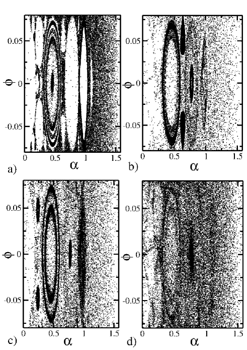
Figure 3: Phase space for the time-dependent stadium billiard. The initial velocities used were (a) $V_{0}=5$, (b) $V_{0}=1.5$, (c) $V_{0}=1.2$ and (d) $V_{0}=0.5$.

Figure 3 shows a phase space for different initial velocities considering both $V_{0}<V_{r}$ and $V_{0}>V_{r}$ for 25 different initial conditions chosen along the chaotic sea. As mentioned before, the phase space may be represented, according to the convenience, either using angular coordinates $\alpha_{n}$ and $\phi_{n}$, or the auxiliary variables $\psi$ and $\xi$. Figure 3 was constructed using $\alpha$ and $\phi$ for $\alpha\in[0,\pi/2]$ and $\phi\in[-\Phi,+\Phi]$. Stickiness regions can be seen in Fig. 3 particularly when the initial velocities are given close but still below to the resonant velocity. As the dynamics evolves, the orbits often change from an island to a surrounding region leading to successive trappings thus not letting the velocity of the particle to reach higher values. For long enough time the orbit chooses (so far a proper mechanism is not yet known) an island and stay there for really long time (as far we have studied, more then $10^{9}$ collisions), as if it was attracted to the fixed point into a stable orbit. The temporally trapping around the stability islands is a possible reason to explain the decay of energy for an ensemble of low energies $(V_{0}<V_{r})$, where many orbits are observed to undergo reduction of energy to an apparently stable state.

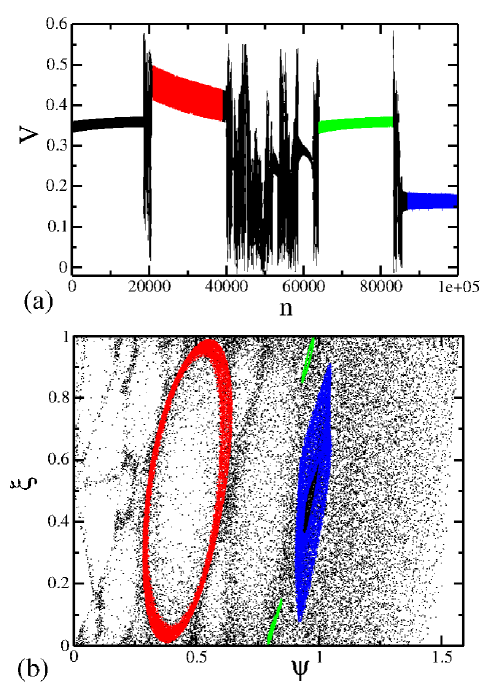
Figure 4: Color Online:Influence of stickiness orbits for the dynamics. In (a) is shown the evolution of the velocity as a function of the number of collisions, and in (b) is shown the same orbit for the coordinates $\psi$ and $\xi$. The initial velocity considered was $V_{0}=0.35$.

The mixed behaviour of the dynamics between quasi-periodic and chaotic region is shown in Fig. 4 where an orbit with initial velocity lower than the resonant one is evolved for a long time leading to temporarily trappings as shown in Figs. 4(a,b). A change in the coordinates of the phase space is made from polar angles $(\alpha,\phi)$ to the auxiliary one $(\psi,\xi)$, with $\xi=0.5+R_{0}\sin(\phi_{n+1})/a$.

3.2 Statistical Analysis

Let us start this section by discussing some statistical analysis concerning behaviour of the average velocity. We consider the quadratic deviation of the average velocity as

$$\omega(n,V_{0})={1\over M}\sum_{i=1}^{M}\sqrt{{\overline{V_{i}^{2}}(n,V_{0})}-{\overline{V_{i}}}^{2}(n,V_{0})}~{},$$ (10)

where $M$ represents an ensemble of initial conditions. The average velocity is given by

$$\overline{V}(n,V_{0})={1\over n}\sum_{i=1}^{n}{V_{i}}~{}.$$ (11)

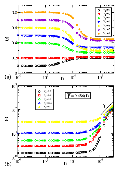
Figure 5: Color Online:Behaviour of $\omega$ as a function of $n$ for ensembles of low and high initial velocities. In (a) all curves experience a decay of energy caused by the successive stickiness trappings while in (b) the curves are experiencing a diffusion in energy leading to Fermi acceleration. They exhibit a growth according a power law with exponent $\beta\approx 0.5$ for long time. The initial velocities are labelled in the figure.

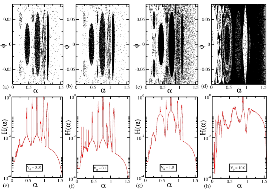
Figure 6: Color Online:Comparison between the final pair of the angular coordinates ($\alpha,\phi$) for both low and high energy ensembles, with the frequency histogram along the whole dynamical evolution of the $\alpha$ coordinate. In (a) and (e) $V_{0}=0.05$, (b) and (f) $V_{0}=0.5$, (c) and (g) $V_{0}=1.0$, and finally in (d) and (h) $V_{0}=10.0$. The histogram axis of (e), (f), (g) and (h) are plotted in logarithmic scale.

Figure 5 shows the evolution of different curves of $\omega$ as a function of $n$ for different initial velocities. Each curve was constructed considering an ensemble of $2000$ different initial conditions chosen along the chaotic sea. They were evolved in time up to $10^{7}$ collisions with the boundary. One sees in Fig. 5(a) all the initial velocities are lower than the resonant one ($V_{0}<V_{r}$) and the $\omega$ curves stay constant for short times. After a crossover they experience a decay for long time series. On the other hand, Fig. 5(b) shows some curves of $\omega$ for initial velocities higher than the resonant one ($V_{0}>V_{r}$). They initially present a constant plateau in the same range of their initial velocities and then suddenly bend towards a growth regime marked by a power law ($\omega\propto n^{\beta}$) with exponent $\beta\approx 0.5$. The $\beta$ exponent on the increments in velocity variables are well described using a central limit theorem (CLT) [54, 55], so that over many time steps, the distribution of displacements is Gaussian with a variance exactly proportional of $\sqrt{n}$ leading to an unlimited growth in the velocity. It is important to emphasize the curves of $\omega$ do not depend on the control parameters $a$, $b$ and $l$ given such parameters produce a behaviour which is scaling invariant [47]. Therefore only one combination of the parameters is enough to have a tendency of the behaviour. The amplitude of the time perturbation is assumed to be constant $B_{0}=0.01$ given it is also scaling invariant [39].

As previously discussed and as is known in the literature, the high initial energy ensembles, those with initial velocity higher than the resonant one, lead to Fermi acceleration [39, 40]. Then we shall give a particular attention and focus on the low energy ensemble therefore characterizing the decay of energy mechanism and its correlation with stickiness orbits. As shown in Fig. 5, the separation of ensembles is seen by considering the averages of different curves of $\omega$. Because the average velocity is one of the observables responsible to characterize the diffusion in energy, a statistical analysis with the average velocity for a grid of initial conditions is a natural and good procedure to quantify the dynamics, particularly the diffusion in energy. It let us to see what initial condition leads to growth or decrease of velocity then defining clearly which one produces Fermi acceleration. We than consider an investigation using the histograms of frequency technique which let us see what region in the phase space produce a larger stickiness, as shown in Fig. 6.

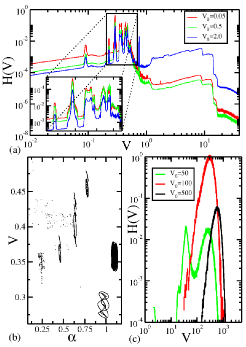
Figure 7: Color Online: In (a) we have the frequency histogram for the lower energy ensemble concerning the whole velocity distribution for $V_{0}=0.05$, $V_{0}=0.5$ and $V_{0}=2.0$. In particular, the zoom-window shows the picks of more intensity. In (b) is shown the convergence velocity as function of the $\alpha$ angle, where we are able to identify in which respective island the orbits got trapped and with respective velocity. And in (c), we show the frequency histogram for the high energy ensemble, where the several peaks of intensity do not appear, and we have a very well defined distribution. Also, the axis of (a) and (c) are in the logarithmic scale, for a better representation of their range and intensity.

We start then considering the angular variables, i.e. the polar angles ($\alpha,\phi$). Since the stadium billiard has an axial symmetry, the variable $\phi$ (or $\xi$), is not a good choice to be considered because it leads to an almost constant distribution along the dynamics. The same process is applied to the auxiliary variable $\xi$. We considered a set of $5\times 10^{6}$ initial conditions chosen along the chaotic sea for both ensembles of high and low energy. Each initial condition was iterated up to $10^{7}$ collisions with the boundary. For the statistical process we collected and saved the final pair of the angular variables at the end of this dynamical evolution. We see from Fig. 6(a,b,c) that for $V_{0}<V_{r}$ the vast majority of points are located inside a stability island. Such region is very close to where the fixed point is in the vicinity of the islands. This final behaviour indeed indicates basically the orbits are trapped inside the stability islands. Alternatively they were attracted to their respective attracting fixed points leading to a clear evidence that the stickiness orbits are responsible for the decay of energy for initial velocities lower than the resonant one. To make a comparison, in Figs. 6(e,f,g) we draw the histograms of frequency of the whole evolution of the $\alpha$ variable along the dynamics for a set of initial conditions ($10^{6}$), but iterated to the same number of collisions and with the same initial velocity of the Figs. 6(a,b,c). We can see some of the preferred regions for the variable $\alpha$, which perfectly match with the position of the islands and the fixed points of the Figs. 6(a,b,c). Particularly the shape of the boundaries of the stability islands are well defined in the histogram of Fig. 6(g). The same procedure is made considering now the high energy ensemble, i.e. for $V_{0}>V_{r}$ as shown in Fig. 6(d). One sees there is no longer convergence to the final pair of angular variables to the regions of the stability islands and fixed points as seen previously. The final pair $(\alpha,\phi)$ just stay wandering along the chaotic sea, a condition that explains why the orbits experience Fermi acceleration. The orbits for $V_{0}>V_{r}$ also experience stickiness, as shown in Fig. 3(a). However these trappings are not sufficient condition to hold their velocity down. Also, in Fig. 6(h), we make the comparison with the whole distribution of the $\alpha$ variable along the whole dynamics, and we can see there is no preferred region anymore. In fact the region in $\alpha$ concerning the chaotic sea shows a growth in the histogram of frequency indicating a high chaotic behaviour therefore corroborating for the FA phenomenon.

After a careful look at histogram of frequency we see some islands are more preferred than others. This explains why in Fig. 5(a) the decay of energy of the curves of $\omega$ produce several different plateaus of convergence for long time which of course depend on the initial velocity. Each of the plateaus are related to the attraction of orbits to the periodic fixed points as shown in Fig. 6. The convergence plateaus are range in a finite region of $V_{final}\in(0.55,0.15)$. In particular the curve of $\omega$ for $V_{0}=0.1$ actually grows for this convergence region. Such region seems to be the same concerning the convergence for final velocity when dissipation is acting in the system [56].

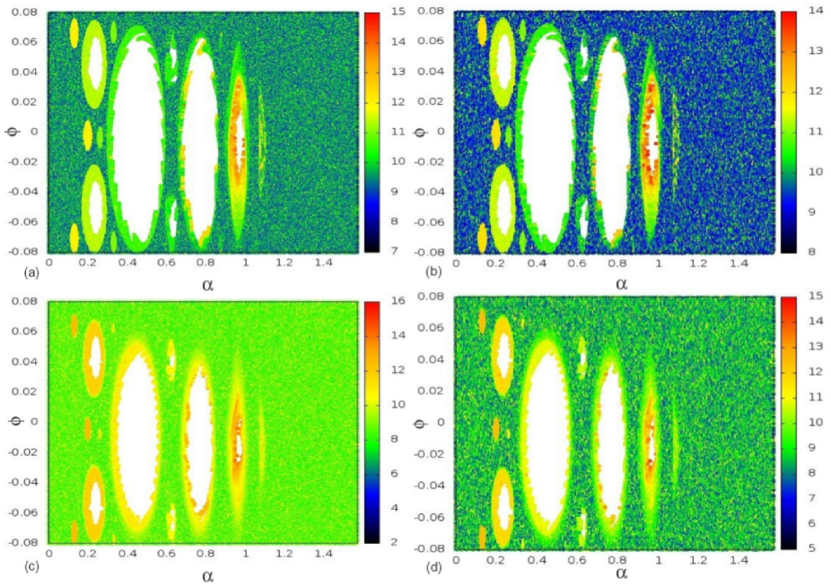
Figure 8: Color Online:Transport analysis considering “real escape” orbits. In (a) and (b), we have $V_{0}=2.0$, and in (c) and (d) we have $V_{0}=1.0$. The color scale represents the escape collision. In (a) and (c) we have the initial conditions that crossed the resonance line and experienced FA, and in (b) and (d), we have the initial conditions that also crossed the resonance line, but experienced decay of energy. Note that the color scale of all figures are in the logarithmic scale, for a better representation of their intensity. Blue (black) indicates a fast escape, and yellow and red (gray and dark gray) represent long times for the orbit to escape. White regions means, that the particle never escaped.

As an attempt to quantify the different plateaus of convergence, we made a histogram of the velocity distribution along the dynamics considering the same ensemble as used to construct Fig. 6 and running the dynamics until $10^{7}$ collisions. Figure 7(a) shows these distributions for three different values of initial velocities. One can see a major concentration for the low energy regime between $0.1$ and $1.0$. Several peaks are noted and decreasing in intensity as the initial velocity increases. Such behaviour is similar as the one shown in the zoom window in Fig. 7(a), even when $V_{0}>V_{r}$, which is the case of $V_{0}=2.0$. Also, for initial velocities lower than the resonant one, there is a distribution for the velocity over $V_{r}$, which is not so intense for $V_{0}=0.05$ and $V_{0}=0.5$ and is quite significant for $V_{0}=2.0$. These distributions confirm what was supposed previously and not all initial conditions for $V_{0}<V_{r}$ experience decay of energy. In a complementary way, not all initial conditions with $V_{0}>V_{r}$ lead to unlimited energy growth. Figure 7(b) shows the distribution of velocities for lower energy regime as a comparison with their positions concerning the polar angular coordinate $\alpha$. This comparison allow us to distinguish in which island of the phase space the orbits will converge to for every range of final velocities plateaus. For example, a comparison between Fig. 7(a) and Fig. 7(b) shows higher intensity peaks for velocities between $V\approx 0.29$ and $V\approx 0.35$. They indicate the orbits prefer to stay in the last two period-one islands of the phase space i.e., the ones located near $\alpha\approx 0.97$ and $\alpha\approx 1.10$ respectively. Finally for Fig. 7(c) we show the histogram of frequency for the high energy ensemble of initial velocities. One can notice that the several peaks are not observed anymore. Now we have a very well defined distribution along the velocities meaning that for the very high energy ensemble, as for example the initial velocities at least ten times larger than $V_{r}$, FA is inherent in the system. Only very few orbits lead to a decay in energy, as shown in the green curve in Fig. 7(c) for $V_{0}=50$. We believe that the period-1 islands should be the preferred ones. All the results come from the resonance velocity, which marks the transition from the Fermi acceleration regime and the decay of energy. The analytical expression, were obtained considering the resonance around the period-1 islands. Also, they are the biggest ones in the phase space, and show themselves more influential for the stickiness phenomenon. You could find different resonance velocities, for different islands of different periods, but even so the period-1 islands should be the more influential ones. Still, one thing that might change the preference between the islands, would be change the value of the geometric control parameters. This change, would influence on the number of islands, and also change the resonance velocity. See Refs.[39, 47].

3.3 Transport analysis

Let us now map along the phase space the initial conditions that lead to unlimited growth of energy and those producing the decay of energy. To start with we consider an ensemble of initial conditions along the phase space uniformly distributed over $\alpha$ and $\phi$ assuming velocities either below $V_{0}<V_{r}$ and above $V_{0}>V_{r}$ the resonant. We look at the time evolution of each initial condition mapping then those who cross the resonant velocity either coming from above showing a decay of energy or coming from below therefore leading to unlimited energy growth

Considering a distribution of initial conditions equally distributed in $2000$ bins along as $\alpha\in[0,\pi/2]$ and $\phi\in[-\Phi,+\Phi]$, we evaluated the dynamics considering an introduction a hole in the system [57, 58, 59, 60, 61] placed concerning the resonance velocity $V_{r}=1.2$. If an initial condition started with $V_{0}<V_{r}$ achieves energy enough to cross the resonant velocity we consider it has escaped from the low energy region to a higher energy region. The same procedure applies for initial conditions in the high energy regime. So if it decays to a velocity smaller than $V_{r}$ we consider it has escaped from high energy to lower energy region. We emphasize the multiple crossings from same orbit can in principle happen so we are considering just the first crossing with $V_{r}$ line, up to the maximum collision of $5\times 10^{6}$.

Figure 8 shows a grid of initial conditions selected near the critical region leading to “escape” in a color scheme. Figures 8(a,b,c,d) then represent in the color scale the respective collision (in a log scale) where an initial condition has crossed the critical resonance velocity line for the first time. Blue (black) indicates fast escape, while yellow and red (gray and dark gray) denotes long time until the orbit crosses the critical line. White regions mean that the orbits never escaped. One can see an existence of orbits trapped by stickiness near the islands concerning Fig.8(a,b,c,d), indicated by yellow and red (gray and dark gray) colors. Indeed these quasi-periodic orbits produce a delay in the diffusion along the energy/velocity axis and hence in the escape through the resonant velocity, leading to a delay also in Fermi acceleration, also, they are more numerous and influential for $V_{0}<V_{r}$.

Considering first an initial velocity $V_{0}=2.0$, we marked the initial conditions that escaped and reached high velocities up to the end of the simulation in Fig.8(a). In the same way the initial conditions that had escaped and experienced the decay of energy up to the end of the simulations are drawn in Fig. 8(b). The same process was made for an initial velocity $V_{0}=1.0$, where the initial conditions that escaped and acquired high velocities are drawn in Fig.8(c), and finally the initial conditions that escaped but remained at the end of the dynamics under the influence of the decay of energy are represented in Fig.8(d).

The fraction of initial conditions of $V_{0}=2.0$ in Figs.8(a,b) is: $14.06\%$ escaped and decreased their velocity up to the end of simulations; $43.63\%$ escaped and experienced FA and the $42.31\%$ never crossed the critical line of resonance velocity. These results indicates that the great majority of initial conditions for $V_{0}=2.0$ stays in the high energy regime. Considering now the fraction of initial conditions of $V_{0}=1.0$ given by Figs.8(c,d) we found that: $55.41\%$ of the initial conditions who had escaped stays in the low energy regime up to the end of simulations, $24.04\%$ escaped and had experienced FA in the end of the simulations, and $20.55\%$ never escaped. These results mean that for the initial conditions of $V_{0}=1.0$, about $80\%$ of the orbits stay confined in the lower energy regime. In particular, for all items of Fig.8, one can see a strong stickiness regime in the last two islands, which are the islands of main influence for the convergence of orbits, as shown in Fig.7. This strong stickiness indicates that these orbits were trapped for really long times around that regions, and crossed the critical resonance line in a very later time, or not even crossed it, which can be an evidence that they were captured by the fixed points, what will lead their velocity down.

4 Final Remarks and Conclusions

We revisited the problem of the time-dependent stadium-like billiard aiming to understand and quantify the mechanism that is responsible for the decay of energy. A non-linear mapping was constructed considering distinct kinds of collisions with the boundary to describe the dynamics. A resonance between the period of oscillation of the boundary and the rotation period around the fixed point was confirmed. Through this resonance two ensemble regimes can be defined at low and high energy, where for high velocities FA is inherent.

A statistical and transport investigation along the phase space was made concerning both regimes of initial energy as an attempt to describe the competition between the decay of energy and FA. We characterize the fundamental role of stickiness and initial conditions for the existence of Fermi acceleration.

Focusing on the lower energy regime, we have seen that stickiness orbits lead the velocity to decay, and for long time the dynamics is stable where most of the orbits are located very close to the fixed points, where it seems that they were captured by fixed points, as if the dynamics was under the influence of dissipation and then suppressing the velocity. The results give support to new studies on stickiness influence in the FA and diffusion process concerning systems with mixed properties in the phase space. Also, it would be interesting to investigate, if stickiness should play similar role in other billiards and chaotic systems.

References

- [1] Hilborn R C 1994, Chaos and Nonlinear Dynamics: An Introduction for Scientists and Engineers, Oxford University Press, New York.
- [2] Lichtenberg A J and Lieberman M A 1992, Regular and Chaotic Dynamics. Appl. Math. Sci. 38, Springer Verlag, New York.
- [3] Zaslasvsky G M 2007, Physics of Chaos in Hamiltonian Systens, Imperial College Press, New York.
- [4] Zaslasvsky G M 2008, Hamiltonian Chaos and Fractional Dynamics, Oxford University Press, New York.
- [5] Scheneider J, Tél T and Neufeld Z 2007, Chaos 17, 3.
- [6] Portela J S E, Caldas I L and Viana R L 2011, Int. J. Bifurcation and Chaos 17, 4067.
- [7] del-Castillo-Negrete D, Carreras B A, and Lynch V E 2005, Phys. Rev. Lett. 94, 065003.
- [8] Jimenez G A and Jana S C 2007, Composites: Part A 38, 983.
- [9] He P, Ma S, and Fan T 2013, Chaos 22, 043151.
- [10] Andersen M F, Kaplan A, Grn̆zweig T, and Davidson N 2006, Phys. Rev. Lett. 97, 104102.
- [11] Abraham N B and Firth W J 1990, J. Opt. Soc. Am. B 7, N.6, 951.
- [12] Milner V, Hanssen J L, Campbell W C and Raizen M G 2001, Phys. Rev. Lett. 86, 1514.
- [13] Tanner G and Søndergaard N 2007, J. Phys. A 40, 443.
- [14] Stein J and Støckmann H J 1992, Phys. Rev. Lett. 68, 2867.
- [15] Sirko L, Koch P M, and Blümel R 1997, Phys. Rev. Lett. 78, 2940.
- [16] Haake F 2001, Quantum Signatures of Chaos Springer, Berlin.
- [17] Ponomarenko L A, Schedin F, Katsnelson M I, Yang R, Hill E W, Novoselov K S and Geim A K 2008, Science, 320, 356.
- [18] Berggren K F, Yakimenko I I and Hakanen J 2010, New J. of Phys. 12, 073005.
- [19] Jalabert R A, Stone A D and Alhassidd Y 1992, Phys. Rev. Lett. 68, 3468.
- [20] de Menezes D D, Jar e Silva M and de Aguiar F M 2007, Chaos 17, 023116.
- [21] Meza-Montes L and Ulloa S E 1997, Phys. Rev. E 55, R6319.
- [22] Xavier E P S, Santos M C, Dias da Silva L G G V, da Luz M G E and Beims M W 2004, Physica A 342, 377.
- [23] Oliveira H A, Manchein C and Beims M W 2008, Phys. Rev. E 78, 046208.
- [24] Zharnitsky V 1995, Phys. Rev. Lett. 75, 4393.
- [25] Fermi E 1949, Phys. Rev. 75, 1169.
- [26] Chernov N and Markarian R 2006, Chaotic Billiards. American Mathematical Society, Vol. 127.
- [27] Loskutov A, Ryabov A B and Akinshin L G 2000, J. Phys. A 33, 7973.
- [28] Loskutov A, Ryabov A B and Akinshin L G 1999, J. Exp. and Theor. Phys. 89, 966.
- [29] Lenz F, Diakonos F K and Schmelcher P 2008, Phys. Rev. Lett. 100, 014103.
- [30] Lenz F, Petri C, Koch F R N, Diakonos F K and Schmelcher P 2009, New J. Phys. 11, 083035.
- [31] Leonel E D and Bunimovich L A 2010, Phys. Rev. Lett. 104, 224101.
- [32] Livorati A L P, Kroetz T, Dettmann C P, Caldas I L and Leonel E D 2012, Phys. Rev. E 86, 036203.
- [33] Manchein C, Beims M W and Rost J M 2014 Physica A 400, 186.
- [34] Bunimovich L A and Vela-Arevalo L V 2012, Chaos 22, 026103.
- [35] Zaslavsky G M and Edelman M 2005, Phys. Rev. E 72, 036204.
- [36] Szezech J D, Caldas I L, Lopes S R, Viana R L, and Morrison J P 2009, Chaos 19, 43108.
- [37] Altmann E G, Motter A E and Kantz H 2006, Phys. Rev. E 73, 026207.
- [38] Custódio M S and Beims M W 2011, Phys. Rev. E 83, 056201.
- [39] Livorati A L P , Loskutov A and Leonel E D 2012, Physica A 391, 4756.
- [40] Loskutov A and Ryabov AB 2002, J. Stat. Phys. 108 995.
- [41] Loskutov A, Ryabov A B and Leonel E D 2010, Physica A 389, 5408.
- [42] Ryabov A B and Loskutov A 2010, J. Phys. A 43, 125104.
- [43] Loskutov A and Ryabov A B 2001, Int. J. of Comp. Anticipatory Syst. 8, 336.
- [44] Loskutov A, Akinshin L G and Sobolevsky A N 2011, Appl. Nonlin. Dyn. 9, 50.
- [45] Bunimovich L A 1979, Commun. Math. Phys. 65, 295.
- [46] Bunimovich L A 1991, Chaos 1, 187.
- [47] Livorati A L P, Loskutov A and Leonel E D 2011, J. Phys. A, 44, 175102.
- [48] Leonel E D 2007, J. Phys. A: Math. Theor. 40, F1077.
- [49] Leonel E D and Livorati A L P 2008 Physica. A 387 1155.
- [50] Livorati A L P, Ladeira D G and Leonel E D 2008 Phys. Rev. E 78 056205.
- [51] Leonel D E and Marinho E P 2009, Physica A 388, 4927.
- [52] Tavares D F and Leonel E D 2008, Braz. J. Phys. 38, 58.
- [53] Tavares D F, Leonel E D and Costa Filho R N 2012, Physica A 391, 5366.
- [54] Adams W J 2009, The Life and times of the Central Limit Theorem. 2.ed. American Mathematical Society, Providence.
- [55] Fischer H 2011, History of the Central Limit Theorem. Springer, New York.
- [56] Livorati A L P, Caldas I L and Leonel E D 2012, Chaos 22, 026122.
- [57] Altmann E G, Portela J S E and Tél T 2013, Rev. Mod. Phys. 85, 869.
- [58] Leonel E D and Dettmann C P 2012, Phys. Lett. A 376, 1669.
- [59] Dettmann C P and Georgiou O 2011, J. Phys. A 44, 195102.
- [60] Dettmann C P and Georgiou O 2009 , Physica D 238, 2395.
- [61] Dettmann C P and Leonel E D 2012, Physica D 241, 403.