GAMMA-RAY EMISSION IN DISSIPATIVE PULSAR MAGNETOSPHERES:
FROM THEORY TO FERMI OBSERVATIONS

Abstract

We compute the patterns of $\gamma$-ray emission due to curvature radiation in dissipative pulsar magnetospheres. Our ultimate goal is to construct macrophysical models that are able to reproduce the observed $\gamma$-ray light-curve phenomenology recently published in the Second Fermi Pulsar Catalog. We apply specific forms of Ohm’s law on the open field lines using a broad range for the macroscopic conductivity values that result in solutions ranging, from near-vacuum to near Force-Free. Using these solutions, we generate model $\gamma$-ray light curves by calculating realistic trajectories and Lorentz factors of radiating particles, under the influence of both the accelerating electric fields and curvature radiation-reaction. We further constrain our models using the observed dependence of the phase-lags between the radio and $\gamma$-ray emission on the $\gamma$-ray peak-separation. We perform a statistical comparison of our model radio-lag vs peak-separation diagram and the one obtained for the Fermi standard pulsars. We find that for models of uniform conductivity over the entire open magnetic field line region, agreement with observations favors higher values of this parameter. We find, however, significant improvement in fitting the data with models that employ a hybrid form of conductivity; specifically, infinite conductivity interior to the light-cylinder and high but finite conductivity on the outside. In these models the $\gamma$-ray emission is produced in regions near the equatorial current sheet but modulated by the local physical properties. These models have radio-lags near the observed values and statistically best reproduce the observed light-curve phenomenology. Additionally, these models produce GeV photon cut-off energies.

1. INTRODUCTION

Almost half a century since the discovery of Pulsars (Hewish et al., 1968) the origin of their emission still remains uncertain. This uncertainty derives both from our lack of knowledge of the precise magnetospheric structure, the location of the radiation emission region and also from the lack of knowledge of the microphysical processes that produce the acceleration of the radiating particles. However, progress has recently been achieved on some of these issues.

For years the only known solution (analytic though) of the pulsar magnetosphere was that of the retarded, inclined vacuum dipole (Deutsch, 1955, hereafter, VRD). However, it was apparent from the very beginning that this solution was unrealistic because it produced huge electric fields with a component $E_{\parallel}$ parallel to the magnetic field on the surface of the star. Such fields would not only pull charges off the surface of the star but would also initiate pair cascades that would fill the magnetosphere with the number of charges necessary to short out these fields everywhere in the magnetosphere (Goldreich & Julian, 1969). The charge density needed to achieve this is known as the Goldreich Julian density $\rho_{\rm GJ}$ and the solutions with $E_{\parallel}=0$ are known as Force-Free Electrodynamic solutions (hereafter, FFE). These FFE magnetospheres represent mathematically the simplest such structures, in the sense that in the axisymmetric case they can be reduced to a single equation for the poloidal magnetic flux, the so-called pulsar equation (Scharlemann & Wagoner, 1973). Even in this simplest of cases, the structure of the magnetosphere remained unknown because the pulsar equation is singular on the Light Cylinder (hereafter, LC), a fact that stymied efforts to obtain numerical solutions.

The situation changed fifteen years ago when the first solution of the pulsar equation that smoothly crossed the singular LC surface was produced by Contopoulos, Kazanas, & Fendt (1999) (hereafter, CKF). This solution determined, by numerical iteration, the poloidal current distribution on the LC that allows a smooth transition of the magnetic field lines across this surface. In addition to the field structure of the magnetosphere, this solution determined the global current structure that flows through the entire magnetosphere and also the local sign of its carriers. Because of the current flow through the magnetosphere, any global solution must inherently provide current closure. Thus, the CKF solution revealed the global current flow of these magnetospheres: The current flows out mainly on a current sheet along the last closed field surface (separatrix) interior to the LC and the equatorial plane beyond the LC (there is also some distributed current above this surface), while the return current flows mainly along the dipole/rotational axis. The axisymmetric solution has since been confirmed and further studied by several others (Gruzinov, 2005; Timokhin, 2006; Komissarov, 2006; McKinney, 2006; Uzdensky, 2003; Yu, 2011; Parfrey et al., 2012).

The FFE magnetospheric solution set was completed when Spitkovsky (2006), using a time-dependent code, numerically integrated Maxwell’s equations appropriate for a rotating, oblique dipole (along with the proper boundary conditions on the surface of the star) to produce the first three-dimensional (hereafter, 3D) pulsar solutions. These solutions reproduced the closed-open magnetosphere configuration of CKF extending the solution to an oblique magnetic geometry.

Kalapotharakos & Contopoulos (2009) and Pétri (2012) confirmed the structure of these 3D solutions. The former used a time-dependent 3D scheme similar to that of Spitkovsky (2006) but with the incorporation of Perfectly Matched Layer (Berenger, 1994, 1996) at the outer boundary of their computational domain, a technique that minimizes the reflected waves at this boundary; this allowed them to follow their simulations for many stellar periods out to distances $r\simeq 10\,R_{\rm LC}$ (where $R_{\rm LC}$ is the LC radius). The latter used a time-dependent pseudo-spectral 3D scheme where they applied the Characteristic Compatibility Method in order to avoid the inward reflection at their outer boundaries. The main features of the 3D ideal FFE solutions have also been confirmed by recent relativistic magnetohydrodynamic models that inherently take into account plasma inertia and pressure (Tchekhovskoy et al., 2013).

Similarly to the CKF, the 3D solutions also comprise an (undulating) equatorial current sheet outside the LC that survives to large distances (Kalapotharakos, Contopoulos, & Kazanas, 2012a), while its shape is similar to that of the split monopole solution current sheet (Bogovalov, 1999). However, within the LC, as the inclination angle $\alpha$ increases, a progressively smaller fraction of the return current reaches the surface of the star through the current sheet. For $\alpha=90^{\circ}$ all the current reaching the stellar surface is distributed over half of the polar caps (Bai & Spitkovsky, 2010). This means that, for $\alpha=90^{\circ}$, the equatorial current sheet outside the LC is not directly connected to the star.

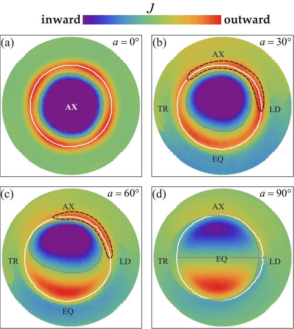
In Fig. 1 we plot, in a color scale, the poloidal current density $J_{p}$ distribution on the polar cap for the indicated $\alpha$ values. The solid white line in all panels denotes the polar cap rim. The open (closed) field lines start inside (outside) this rim. We note that any FFE simulation could have magnetic field lines that close outside the LC due to unavoidable numerical dissipation. Nonetheless, we define open magnetic field lines to be those that cross the LC. In each panel there are notations that indicate the directions (with respect to the magnetic axes) toward the leading edge (LD), the rotational axis (AX), the trailing edge (TR), and the rotational equator (EQ). This notation scheme is followed in all the subsequent figures (whenever is needed). The positive values (reddish color) of $J_{p}$ indicate outward current while the negative (blueish color) values indicate inward current. The solid gray line is the zero current density line ($J_{p}=0$). We see that for $\alpha=0^{\circ}$ (Fig. 1a) there is a current sheet all along the separatrix (the white rim). However, for $\alpha>0$ (Figs. 1b,c,d) only a part of the return current reaches the stellar surface in a current sheet form (the areas within the dashed black lines). These areas are toward the rotational axis and mostly toward the leading side of the polar cap, becoming progressively smaller as $\alpha$ increases. This effect makes, in general, asymmetric the structure from both sides of the equatorial current sheet.

One should note here that both the analytic VRD and the numerical FFE solutions are dissipationless and so, strictly speaking, preclude the acceleration of particles and the emission of radiation (Kalapotharakos et al., 2012c). The VRD solutions have huge $E_{\parallel}$ but no particles ($\rho=0$) to accelerate, while the FFE solutions have large values of the charge density $\rho$ which however shorts-out the accelerating electric field $E_{\parallel}$ yielding again no acceleration. The observed, radiation-emitting pulsars should therefore lie somewhere between these two limiting regimes.

More recently, two groups (Kalapotharakos et al., 2012c; Li et al., 2012b) began filling the solution gap between the VRD and FFE by producing solutions with both $\rho\neq 0$ and $E_{\parallel}\neq 0$. In order to proceed this way, one needs a macroscopic prescription for the current density $J$, i.e. a form of Ohm’s law. The actual Ohm’s law is expected to be rather complicated incorporating many effects (e.g., pressure, inertia, Hall; see Meier, 2004) and taking into account also any pair production microphysical processes. The adopted prescriptions, in the current study, even though simplistic, provide solutions that have a distribution of non-zero $E_{\parallel}$. All these prescriptions eventually involve a conductivity parameter $\sigma$ (expressed in units of the fundamental frequency in the problem, namely the pulsar rotation frequency $\Omega$) that describes the plasma’s ability to screen the accelerating electric fields, with the final solution depending on both the macroscopic prescription for $J$ and the corresponding spatial distribution of $\sigma$. According to most of these prescriptions, as $\sigma$ goes from 0 to $\infty$, an entire spectrum of solutions between VRD and FFE is recovered.

Figure 1.— The distribution of the FFE poloidal current density on the polar caps (colors indicate the magnitude and direction) for the indicated inclination angles $\alpha$. In each panel the white line denotes the polar cap rim while the gray line denotes the zero current line that separates the inward from the outward current. For $\alpha=0^{\circ}$ the return current has a current sheet component all along the separatrix that separates the open from the closed magnetic field lines (strong red color along the white line). This current sheet component connects the equatorial current sheet with the stellar surface. As the inclination angle increases the return current that reaches the stellar surface in a current sheet form (part within the black dashed line) becomes gradually smaller until $\alpha=90^{\circ}$ where the equatorial current sheet is not directly connected to the stellar surface. The notations ‘LD’, ‘AX’, ‘TR’, and ‘EQ’ indicate the directions (with respect to the magnetic axis) toward the leading edge, rotational axis, trailing edge, and rotational equator, respectively. We note that the ‘AX’ direction for $\alpha=0^{\circ}$ and ‘EQ’ direction for $\alpha=90^{\circ}$ coincide with the magnetic axis. The axisymmetric case ($\alpha=0^{\circ}$) is degenerate and the ‘LD’, ‘TR’, and ‘EQ’ directions are not defined.

On the observational side, the launch of Fermi Gamma-Ray Space Telescope ushered in a new era in the study of pulsars. The discovery of over 130 new pulsars to date in high energy ($>100$ MeV) $\gamma$-rays (117 of which are included in the Second Fermi Pulsar Catalog (2PC), Abdo et al., 2013), increased the corresponding data base by twentyfold. The measurement of exponential cut-offs in the pulsar spectra (Abdo et al., 2009) immediately resolved the issue of the location of the high energy $\gamma$-ray emission in favor of the outer magnetosphere. Furthermore, the notable increase in the number of detections allows meaningful statistical studies of their $\gamma$-ray properties and cross-correlations with emission at other wavelengths, most notably with the radio. One of the most important such correlations has been that between the peak-separation $\Delta$ of the $\gamma$-ray pulses and the lag $\delta$ between the $\gamma$-ray and radio emission. This is important because it involves observed quantities across widely separated frequency bands, one of which (radio) is widely accepted as emitted by a region located near the pulsar dipole axis from a region close to the pulsar surface. Since the $\gamma$-ray emission depends more sensitively on the structure of the pulsar magnetic field lines near the LC and $E_{\parallel}$ distribution, the $\Delta-\delta$ diagram can be employed to test the pulsar $\gamma$-ray emission models. The confrontation of pulsar model magnetosphere predictions with the pulsar $\Delta-\delta$ diagram is the essence of the present paper.

In Kalapotharakos et al. (2012b) we presented for the first time $\gamma$-ray light curves based on realistic particle trajectories that take into account the physical properties (i.e. the field structure and the values of $E_{\parallel}$) of dissipative solutions. This study involved only one inclination angle $\alpha=90^{\circ}$ but a wide range of conductivity values. The resulting light curves exhibited double peaked shapes for solutions corresponding to the entire range of $\sigma$ values. It was also shown that as $\sigma$ increases, the corresponding emission region moves outward and for the highest adopted $\sigma$ values (solutions near-FFE) an important $\gamma$-ray component comes from a region near the equatorial current sheet outside the LC. Nevertheless, all these high-conductivity light-curves showed a clear trend for radio-lags larger than those observed. This “lag” problem seems to appear also when the $\gamma$-ray emission is calculated by employing simple phenomenological $\gamma$-ray emission models for particles moving in FFE geometries (Contopoulos & Kalapotharakos, 2010; Bai & Spitkovsky, 2010; Harding et al., 2011).

In this paper, we extend our study of $\gamma$-ray light curves for the entire range of values of the inclination angle $\alpha$. Our goal is to study the radiation patterns of dissipative solutions and to compare statistically the corresponding $\Delta-\delta$ diagrams with those observed. This will reveal whether and under what assumptions the dissipative models can explain the observed phenomenology. Eventually, the macrophysics of the models that passes the comparison test successfully should be related to microphysical mechanisms that can support it.

The structure of the present paper is as follows. In Section 2 we give a brief outline of our dissipative models. In Section 3 we use the field structure of these models to define realistic electron (or positron) trajectories and calculate their corresponding energies (including the effects of radiation losses) and the resulting curvature radiation emission. In Section 4 we present our results. We discuss the particle orbit properties, their evolution with $\sigma$ and how this evolution determines the $\gamma$-ray emission regions and the corresponding light curves. Particular emphasis is given to the comparison between these results and the observational data. In Section 5, guided by the results of Section 4, we present special models corresponding to certain spatial $\sigma$ distributions that are able to reproduce the observed phenomenology. Finally, in Section 6 we present our conclusions.

2. Model Description

In order to produce our models we solve numerically the time dependent Maxwell equations

$$\frac{\partial\mathbf{B}}{\partial t} =-c\boldsymbol{\nabla}\times\mathbf{E}$$ (1)

$$\frac{\partial\mathbf{E}}{\partial t} =c\boldsymbol{\nabla}\times\mathbf{B}-4\pi\mathbf{J}$$ (2)

using a 3D Finite Difference Time Domain technique (Kalapotharakos & Contopoulos, 2009; Kalapotharakos et al., 2012c). We consider the presence of a dipole magnetic moment $\boldsymbol{\mu}$ at the center of the star and that the star itself is a perfect conductor; then the boundary condition on the stellar surface for the electric field reads $\mathbf{E}=-(\boldsymbol{\Omega}\times\mathbf{r})\times\mathbf{B}/c$ , where $\boldsymbol{\Omega}$ is the angular velocity of the neutron star and $\mathbf{B}$ the magnetic field on its surface. The closure of the system then requires a prescription for the current density $\mathbf{J}$ in terms of the fields. For the FFE solutions this is given by (Gruzinov, 1999)

$$\mathbf{J}=c\rho\frac{\mathbf{E}\times\mathbf{B}}{B^{2}}+\frac{c}{4\pi}\frac{\mathbf{B\cdot\nabla\times B-E\cdot\nabla\times E}}{B^{2}}\mathbf{B}$$ (3)

and guarantees that $\mathbf{E_{\parallel}}$, the component of the electric field parallel to $\mathbf{B}$, be identically zero. Numerically, rather than computing the above expression we employ just the drift current (the first term in the above expression) and we force the value of any parallel electric field component at each time step to equal zero. One should note that the charge density $\rho$ in the expression above is given by $\rho=\boldsymbol{\nabla}\cdot\mathbf{E}/(4\pi)$.

As noted above, realistic pulsar magnetospheres must be different from those of FFE to allow for $\mathbf{E_{\parallel}}\neq 0$, needed for the acceleration of particles that produce the observed radiation and, therefore, one is compelled to produced non-FFE models. This is achieved by considering prescriptions for $\mathbf{J}$ different from those of Eq. (3). In Kalapotharakos et al. (2012c) we used the following very simplistic prescription for the current density

$$\mathbf{J}=c\rho\frac{\mathbf{E}\times\mathbf{B}}{B^{2}}+\sigma\mathbf{E_{||}}\,.$$ (4)

The first term is the usual drift component while the second term regulates the $\mathbf{E_{\parallel}}$ through the conductivity $\sigma$. This prescription requires a special treatment that sets $E_{\perp}<B$ securing in that way that the drift component stays always subluminal. This is most important near the equatorial current sheet outside the LC where the magnetic field approaches 0.

We also produced models (Kalapotharakos et al., 2012c) employing the so-called Strong Field Electrodynamics (Gruzinov, 2008, hereafter, SFE) that has a covariant formulation for the current density that reads

$$\mathbf{J}=\frac{c\rho\mathbf{E\times B}+(c^{2}\rho^{2}+\gamma_{f}^{2}\sigma^{2}E_{0}^{2})^{1/2}(B_{0}\mathbf{B}+E_{0}\mathbf{E})}{B^{2}+E_{0}^{2}}$$ (5)

where

$$B_{0}^{2}-E_{0}^{2}=\mathbf{B^{2}-E^{2}},\;B_{0}E_{0}=\mathbf{E\cdot B},\;E_{0}\geq 0$$ (6)

$$\gamma_{f}^{2}=\frac{B^{2}+E_{0}^{2}}{B_{0}^{2}+E_{0}^{2}}~{}.$$ (7)

This prescription as well as the one proposed by Li et al. (2012b)

$$\mathbf{J}=\frac{c\rho\mathbf{E\times B}+\gamma_{f}\sigma E_{0}(B_{0}\mathbf{B}+E_{0}\mathbf{E})}{B^{2}+E_{0}^{2}}~{},$$ (8)

where $E_{0},B_{0}$ and $\gamma_{f}$ are defined by Eqs. (6), (7), have been produced considering Ohm’s law in the fluid frame. However, since this frame is not a priori known, one has to assume a velocity. In SFE the dissipation takes place only in the space-like regions ($J>\rho c$) and the fluid frame is the one for which the charge density vanishes $(\rho=0)$. In prescription (8) the fluid frame is assumed to be the slowest moving one that has electric fields parallel to magnetic fields.

All the above macroscopic prescriptions for the current density $\mathbf{J}$ tend to the FFE prescription Eq. (3) as $\sigma\rightarrow\infty$. Nevertheless, the advantage of (4) and (8) (though still not covariant) is that their corresponding models can span the entire spectrum of solutions between VRD and FFE as $\sigma$ varies from 0 to $\infty$, while SFE produces solutions that have $J\rightarrow\rho c$ as $\sigma\rightarrow 0$. On the other hand, the SFE and (8) naturally include the $E_{0}$ term in the denominator of the drift term that makes the treatment of the region near the current sheets much easier since it never allows the drift current to be superluminal. Moreover, this expression is compatible with the motion of the charged particles along the drift direction. Thus, in the present work we decided to add the $E_{0}$ term in our prescription (4), that now reads

$$\mathbf{J}=c\rho\frac{\mathbf{E}\times\mathbf{B}}{B^{2}+E_{0}^{2}}+\sigma\mathbf{E_{||}}$$ (9)

in order to take advantage of its features on the current sheet and to be consistent to the motion of the particles along the drift direction.

We note that the final solutions we get from prescriptions (4), (8) and (9) do not differ significantly and one can always get the same spatial distribution of $E_{\parallel}$ values just by applying a slightly different value of $\sigma$. However, the distribution of $\sigma$ that determines the potential drops at each region of the magnetosphere, which can reproduce the observed pulsar phenomenology, the ultimate subject of this kind of research, cannot be established beforehand.

Figure 2.— The distribution of the potential drop $V_{B}$ along the magnetic field lines, in the indicated color scale, for $\alpha=15^{\circ}$. In both panels (a) and (b) the black line denotes the polar cap rim for the FFE solution. The red line denotes the polar cap rim for the dissipative solution that has $\sigma=0.02\Omega$ everywhere in the magnetosphere while the green line denotes the polar cap rim for the dissipative solution that has $\sigma=0.02\Omega$ only in the open magnetic field line region and FFE regime for the closed region. We see that the perfectly conductive closed region (b) decreases the potential drop along the open magnetic field lines compared to that of a magnetosphere that is dissipative in both open and closed regions (a). We see also that the green polar cap rim is closer to the red one than it is to the FFE polar cap rim, even though it is larger. We note that for high $\alpha$ the corresponding green line is closer to the corresponding black line.

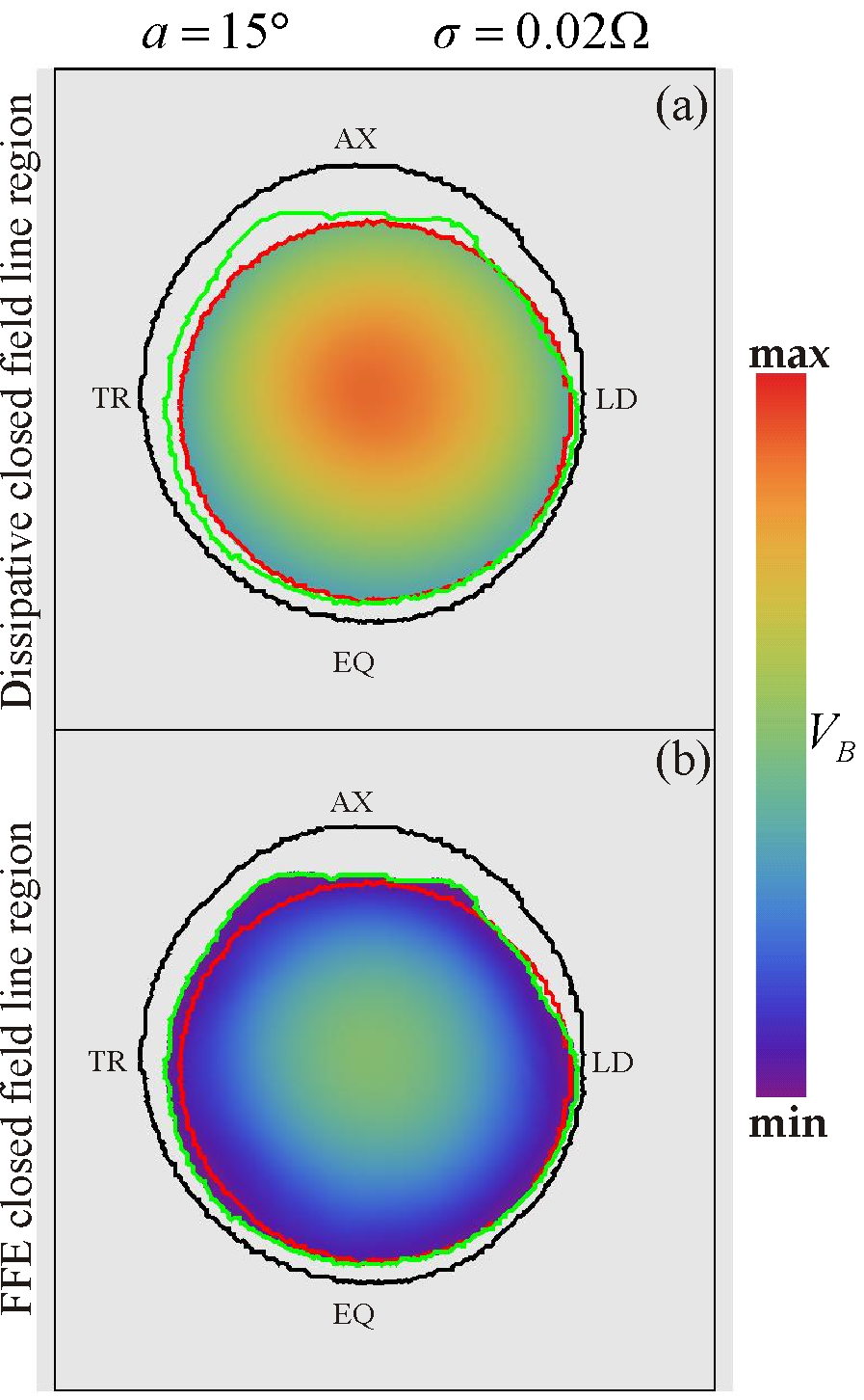
In what follows, we present results produced employing prescription (9) while we have tested that the main results remain unaffected by the use of the other prescriptions. We have also modified our code so that it can identify the different magnetic field lines at each snapshot in time as the pulsar rotates. This allows $\sigma$ to be magnetic-field-line dependent. This technique will be extremely helpful when the microphysical studies will provide all the different plasma properties along the different magnetic field lines. However, this information is still incomplete and so we reserve this kind of study for the future. Nevertheless, we still employ this technique in the present paper in order to produce solutions with different values of $\sigma$ in open and the closed field lines. It is reasonable to consider that the closed field line regions are described by FFE and only the ‘open’ regions may have small $\sigma$ values. Thus, for the solutions presented in the next sections we have always applied very high $\sigma$ value ($\sigma=40\Omega$) for the closed field line regions. Note, that a similar technique has been used by Li et al. (2012a). The difference in that study is that it considers the closed field line regions to be the same as the FFE ones, independently of the value of $\sigma$ in the open field lines. However, this is not strictly speaking correct, because one cannot determine the open-closed field line boundary from a solution that has the same $\sigma$ (however large) over all space, i.e. the FFE solution. Li et al. (2012a) claimed that the spin-down, i.e. the Poynting flux, is relatively insensitive to the size of the conducting closed zone. However, for the current study the detailed determination of the last open field lines and the corresponding voltage along them is, in principle, essential. This effect is more dominant for low $\alpha$ values: In Fig. 2 we plot the polar caps for $\alpha=15^{\circ}$ for $\sigma=0.02\Omega$ applied everywhere in the magnetosphere (red line), for $\sigma=0.02\Omega$ applied only in the open field line region while the FFE (in reality highly conductive) condition is applied in the ‘closed’ region (green line) and for the FFE (everywhere applied) solution (black line). The color scale represents the potential drop $V_{B}$ along the magnetic field lines for the solution with finite conductivity everywhere (Fig. 2a) and for the solution with finite conductivity only in the open field line region (Fig. 2b). We see that the green line is closer to the red line (though still larger) rather than the black one. We note that as we go to high $\alpha$ values the corresponding green line goes closer to the black line.

Another issue is the construction of solutions of very high $\sigma$. This problem arises from the small time steps $dt$ needed to deal with the high $\sigma$ values of the ‘stiff’ second term in all expressions for the current density $\mathbf{J}$. The most general solution of this problem is the use of implicit-explicit integrators (Palenzuela, 2013, and references therein). However, in our case the solutions corresponding to $\sigma\rightarrow\infty$ (FFE) are known. Near this regime (FFE), the solutions have almost identical field structure and the only difference is the spatial distribution of the small $E_{\parallel}$ values. The value $\mathbf{E_{\parallel}}$ is determined by the following equation

$$\frac{\partial\mathbf{E_{\parallel}}}{\partial t}=c(\boldsymbol{\nabla}\times\mathbf{B})_{\parallel}-4\pi\mathbf{J_{\parallel}}$$ (10)

with $\mathbf{J_{\parallel}}$ given by the second term of Eq. (9) and with $(\boldsymbol{\nabla}\times\mathbf{B})_{\parallel}$ given by its FFE value. For $\sigma\rightarrow\infty$, $E_{\parallel}\rightarrow 0$ and $\partial E_{\parallel}/(\sigma\partial t)\rightarrow 0$. This implies that for high enough $\sigma$ the remaining (small) $E_{\parallel}$ can be calculated approximately by setting the right hand side of Eq. (10) equal to 0. This $E_{\parallel}$ value can thus be obtained by the expression

$$E_{\parallel}=\frac{c|(\boldsymbol{\nabla}\times\mathbf{B})_{\parallel}|_{\text{(FFE)}}}{4\pi\sigma}$$ (11)

where the $\boldsymbol{\nabla}\times\mathbf{B}$ is assumed to be the one corresponding to FFE solutions. In case of prescriptions (8) and (5) the $E_{\parallel}$ value can be derived easily either numerically or from the linearized expressions with respect to $E_{\parallel}$. The above approximation implies that for a specific $\sigma$ value, the higher the $(\boldsymbol{\nabla}\times\mathbf{B})_{\parallel}$ the higher the $E_{\parallel}$ will be. In order to confirm this approximation, we ran a few simulations with $\sigma=30\Omega~{}-~{}70\Omega~{}$ using prescriptions (9) and (8) and we compared these models to the corresponding FFE ones that have the approximated spatial $E_{\parallel}$ distributions (e.g. Eq. 11). There were only slight differences between these two configurations that do not affect the trajectories and the corresponding light-curve results we present in the next sections.

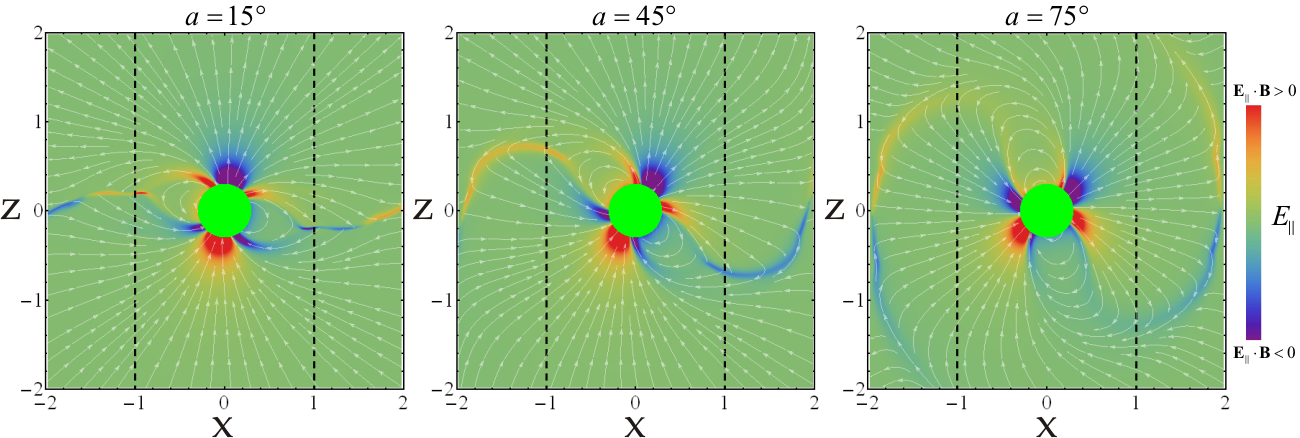
In Fig. 3 we plot, in color scale, and for the indicated $\alpha$ values, the distribution of $E_{\parallel}$ provided by relation (11). In this plot we have considered the same $\sigma$ value (e.g. $\sigma=500\Omega$) everywhere. The blue (red) color implies $E_{\parallel}$ antiparallel (parallel) to the local $B$. The distribution of $E_{\parallel}$ reflects the distribution of $(\boldsymbol{\nabla}\times\mathbf{B})_{\parallel}$ in the corresponding FFE solutions. For the constant $\sigma$ (in the open field zone) solutions, in the remaining of this study we employ approximation (11) for all cases with $\sigma\geq 30\Omega$.

In our simulations we use a stellar radius $r_{\star}=0.2R_{\rm LC}$. Our computational domains extend up to $5R_{\rm LC}$ and the spatial resolution (i.e. the grid cell size) is $0.01R_{\rm LC}$. Each simulation has been evolved for 2-3 stellar rotations. We note that the calculations presented below assume standard values for pulsar period $P_{\star}=0.1s$ and magnetic field on stellar surface $B_{\star}=10^{12}G$.

Figure 3.— The distribution of $E_{\parallel}$, in the indicated color scale, on the poloidal plane $(\boldsymbol{\mu},~{}\boldsymbol{\Omega})$, for very high conductivity values (near-FFE) and for the indicated $\alpha$ values. We see, in general, high $E_{\parallel}$ above the polar caps, near the separatricies, and near the equatorial current sheets outside the light-cylinder (vertical black dashed lines).

3. Realistic Particle Trajectories

In the present paper we study the contribution of curvature radiation to the observed $\gamma$-ray light curves. We define realistic trajectories of charged particles ($e^{-}$ and $e^{+}$) following a methodology similar to that presented in Kalapotharakos et al. (2012b). Assuming that the speed of the particles is always very close to $c$, we set the velocity vector $\mathbf{v}$, everywhere in the magnetosphere, to be

$$\mathbf{v}=\left(\frac{\mathbf{E}\times\mathbf{B}}{B^{2}+E_{0}^{2}}+f\frac{\mathbf{B}}{B}\right)c~{}.$$ (12)

The first term in expression (12) is a drift velocity component similar to that in our $\mathbf{J}$ prescriptions while the second term is a component along the local magnetic field line. The sign and the value of the scalar quantity $f$ is set so that the total speed of the particle be $c$ and the motion be outward. For a given magnetospheric solution (i.e. specific field configuration) the spatial distribution of $f$ is then uniquely determined. This fixes the assumed velocity flow in the entire magnetosphere and hence the particle trajectories. Since the particle trajectories are defined, the only additional requirement for the calculation of the particles’ kinetic energy along their trajectories is their initial conditions (position and energy). Assuming we know these we can calculate the $\gamma_{L}$ values (Lorentz factors) along each trajectory taking into account their acceleration by the $\mathbf{E_{\parallel}}$ provided by the solution and their losses due to curvature radiation. Thus, the calculation of the $\gamma_{L}$ value is made by integration over time of

$$\frac{d\gamma_{L}}{dt}=f\frac{q_{e}cE_{\parallel}}{m_{e}c^{2}}-\frac{2q_{e}^{2}\gamma_{L}^{4}}{3R_{\rm CR}^{2}m_{e}c}$$ (13)

where $q_{e}$ and $m_{e}$ are the electron charge and rest-mass, respectively while the quantity $R_{\rm CR}$ is the radius of curvature at each point of the trajectory. The first term in (13) formulates the energy gain rates of the particles due to the parallel electric field component they encounter along their trajectories and the second term formulates the energy loss rates due to curvature radiation.

Below, whenever it is not stated otherwise, the radiating particles are considered to start on the stellar surface, distributed uniformly on the polar cap with small $\gamma_{L}$ values ($\gamma_{L}<100$). In each model, we integrated $\approx 2\times 10^{6}$ trajectories originating on each polar cap. We have checked that this number ensures a reliable statistics and provides robust results. We note, also, that at each point of the stellar surface we assume that we have the kind of particles ($e^{-},e^{+}$) needed in the region to accelerate outward. We integrate these trajectories up to $r=2.5R_{\rm LC}$, we collect the bolometric energy along the emitting directions (locally tangential to the trajectories) and taking into account the time-delay effects, we construct sky-maps and the corresponding light-curves.

Figure 4.— Trajectories and emission level (in the indicated color scale) for $\alpha=45^{\circ}$ and for different $\sigma$ values. (Left hand column) We plot the particle trajectories in the corotating frame together with the equatorial current sheet. The color along the orbits represents the local emissivity due to curvature radiation $\propto\gamma^{4}R_{\rm CR}^{-2}$. (Middle column) The same trajectories but in the inertial frame. (Right hand column) A sampling of points that trace the comoving (prescribed by the particle flux) magnetosphere volume contributing to the highest 95% of the total emission. We note that each of these points represent the same number of particles and not equal volume elements. All columns show that as $\sigma$ increases the emission moves gradually outward and for high $\sigma$ values it is produced in regions near the equatorial current sheet outside the light-cylinder. We note also that the trajectories for $\sigma\geq 30\Omega$ are almost identical since for these $\sigma$ values the field structure remains almost the same and the particles are near corotation along the magnetic field lines.

4. Results

4.1. Radiation patterns

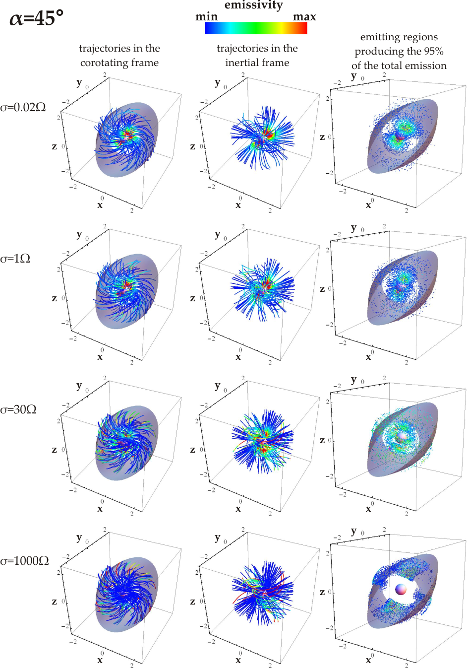
In the left-hand column of Fig. 4 we plot, for $\alpha=45^{\circ}$ and for the indicated $\sigma$ values, a sample of 200 particle trajectories in the corotating frame. The gray transparent surface represents the equatorial current sheet outside the LC as it is defined in the corresponding FFE solution. The color along each trajectory represents the local emissivity ($\propto\gamma_{L}^{4}R_{\rm CR}^{-2}$) according to the indicated color scale. In the middle column, the same trajectories are plotted but in the inertial frame. We note that the trajectories, for high $\sigma$ follow very closely the magnetic field lines in the corotating frame while the trajectories of low $\sigma$ deviate from them since the first term of the right-hand side of Eq. (12) no longer supports corotation. For low $\sigma$ we see significant radiation (reddish color) at low altitudes, well within the LC. However, as $\sigma$ increases radiation starts being produced at higher altitudes. Thus, the higher the value of $\sigma$, the higher is the altitude along each trajectory at which most of the emission is produced. This happens because as $\sigma$ increases $E_{\parallel}$ decreases and so the particles need to traverse longer distances to reach the $\gamma_{L}$ values that allow them to radiate efficiently. Moreover, the trajectories that produce significant emission in the outer parts of the magnetosphere seem to be those moving in regions near the equatorial current sheet in the corotating frame (see left-hand column of Fig. 4). In the right-hand column we plot, in the corotating frame, the points that trace the comoving volume (prescribed by the particle flux) where the highest 95% of the total emission of the entire magnetosphere is produced. The color of individual points still represents the corresponding emissivity. These figures show that for low $\sigma$ almost all the emission comes from the inner magnetosphere from lobes above the magnetic poles. For higher $\sigma$ these lobes change their orientation slightly and become progressively smaller with $\sigma$. At the same time more and more points from the outer magnetosphere contribute to the total emission. These (outer) points, for high $\sigma$ ($\sigma>1\Omega$) lie in regions close to the equatorial current sheet. Actually, for very high $\sigma$ values the inner magnetosphere has no significantly radiating points and all the emission is produced in the outer magnetosphere in regions near the equatorial current sheet.

Figure 5.— The radius of curvature $(R_{\rm CR})$ measured in light-cylinder radii for $\alpha=45^{\circ}$ and for the indicated $\sigma$ values. (Top row) We plot the $\log(R_{\rm CR})$ vs spherical radius $r$ (measured in light-cylinder radii) along many particle trajectories that start on the corresponding polar caps. We see that $R_{\rm CR}\propto 10^{r}$ with a scatter of one order of magnitude. (Bottom row) The $\log(R_{\rm CR})$ values of particle trajectories at $r=1R_{\rm LC}$ mapped (in the indicated color scale) on the corresponding polar caps. We see that particles trajectories that start near the polar cap edges have smaller $R_{\rm CR}$ values.

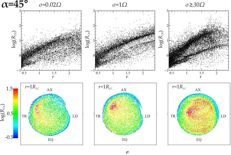
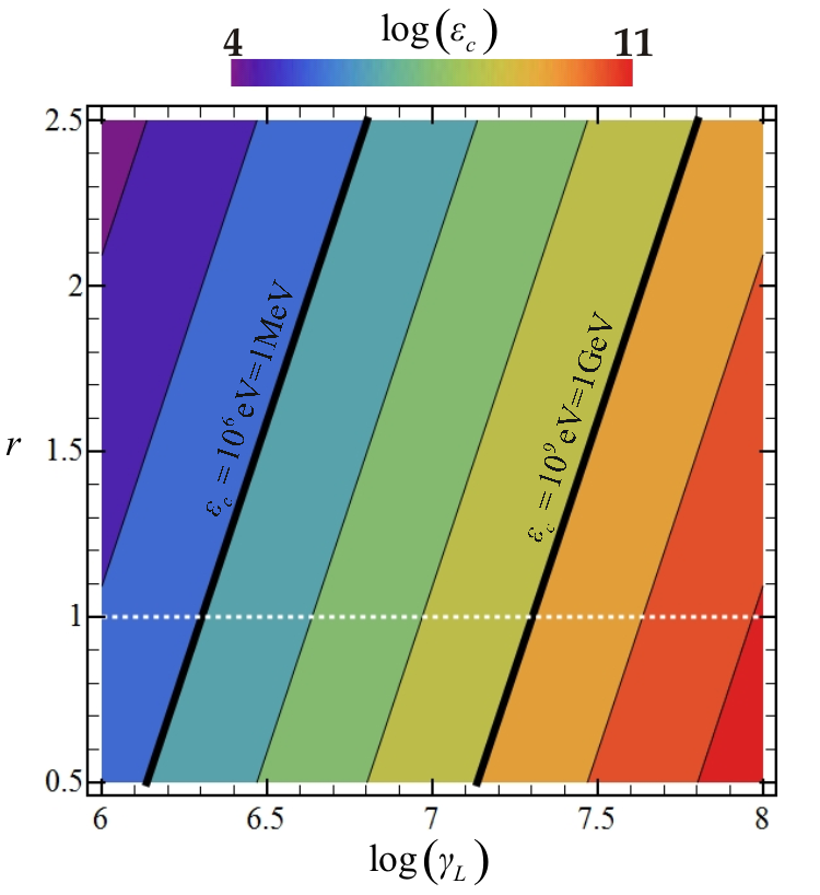
The local emissivity is more sensitive to the local values of $\gamma_{L}$ than the corresponding values of $R_{\rm CR}$. In turn, the local values of $\gamma_{L}$ are very sensitive to the values of $E_{\parallel}$ that the particles see up to a specific point, while $R_{\rm CR}$ is not as sensitive to $E_{\parallel}$ but depends mostly on the geometry of the magnetic field lines. Actually, $R_{\rm CR}$ remains almost unchanged beyond some not extremely high value of $\sigma$. In the first row of Fig. 5 we plot, for $\alpha=45^{\circ}$ and for the indicated values of $\sigma$, the values of $\log(R_{\rm CR})$ versus the spherical radius $r$ for many points along a large sample of particle trajectories. We see that, in general, $\log(R_{\rm CR})$ increases almost linearly with $r$, even though there is a dispersion of $\log(R_{\rm CR})$ values that scatters the corresponding $R_{\rm CR}$ values within 1-2 orders of magnitude. The radius of curvature can be approximated by the expression $R_{\rm CR}\propto 10^{r}$. For a specific $r$ the larger $R_{\rm CR}$ values correspond to the inner region of the polar cap while the smaller ones come from trajectories originating near the polar cap rim (last open field lines). In the second row of Fig. 5 we map on the polar cap, in the indicated color scale, the values of $\log(R_{\rm CR})$ that these trajectories reach at $r=1R_{\rm LC}$. These plots show clearly that $R_{\rm CR}$ increases slightly with $\sigma$. Moreover, we see that the small $R_{\rm CR}$ values are always for trajectories that originate near the polar cap edge. This can be also observed in the middle column of Fig. 4, where it is clear that the trajectories that start near the edge of the polar cap are much more curved (i.e. smaller $R_{\rm CR}$) than the trajectories originating inside the polar cap rim. This implies that the high emission observed in regions near the equatorial current sheet, in the high $\sigma$ models is additionally enhanced by the smaller values of $R_{\rm CR}$ of these trajectories. The general properties and trends presented in Figs. 4, 5 remain the same for all values of the pulsar inclination angle $\alpha$. The $R_{\rm CR}$ values and their dependence on $r$, solely determined by the field structure, put certain restrictions on the location where specific photon energies could be produced. The cut-off energy in the curvature radiation spectrum is given by

$$\epsilon_{c}=\frac{3}{2}c\hbar\frac{\gamma_{L}^{3}}{R_{\rm CR}}.$$ (14)

Figure 6 is a contour plot of $\log(\epsilon_{c})$ in the $r-\log(\gamma_{L})$ plane. In this plot we have considered that $R_{\rm CR}=0.05\times 10^{r}$ (an approximate expression that describes the lower segment of the points plotted in Fig. 5 for $\sigma\geq 30\Omega$). The two thick black lines denote the indicated $\epsilon_{c}$ values (1MeV and 1GeV) while the horizontal dashed white line denotes the $r=1R_{\rm LC}$ value. Figure 6 shows the minimum $\gamma_{L}$ value required for a specific photon energy to be emitted at a particular distance. For example, in order to have GeV photon emission at $r=1R_{\rm LC}$ the emitting particles must have Lorentz factors at least $\gamma_{L}=10^{7.3}$ (at this distance).

Figure 6.— The cut-off energy $\epsilon_{c}$ in the indicated logarithmic scale as a function of $\log(\gamma_{L})$ and $r$. The two thick black lines denote the 1Mev and 1GeV $\epsilon_{c}$ values, as indicated in the figure. The white dashed horizontal line denotes the $r=1R_{\rm LC}$ value. There are restrictions with respect to the minimum $\gamma_{L}$ values required for certain photon energy emission at some distance.

Figure 7.— Radiation patterns and $\gamma_{L}$ values for $\alpha=75^{\circ}$ and for the indicated $\sigma$ values. (Left hand column) The maximum $\gamma_{L}$ values of particle trajectories up to $r=2.5R_{\rm LC}$ mapped, in logarithmic color scale, on the corresponding polar caps. For low $\sigma$ values the $\gamma_{L_{max}}$ values can reach higher than $10^{8}$ while for very high $\sigma$ values hardly exceed $10^{6}$. (Middle column) The total emission values along the particle trajectories up to $r=2.5R_{\rm LC}$ mapped, in the indicated color scale, on the corresponding polar caps. We see that the high total emission values move from the inner part of the polar cap toward its edge. Note that in these panels we plot a sampling of points $(\approx 10^{4})$ that is 1/200 of the total number $(2\times 10^{6})$ of particle trajectories we have integrated in each polar cap. (Right hand column) The corresponding sky-maps: the luminosity per solid angle $dL/d\omega$, in the indicated color scale as a function of the rotation phase $\phi_{ph}$ and the observer inclination angle $\zeta$.

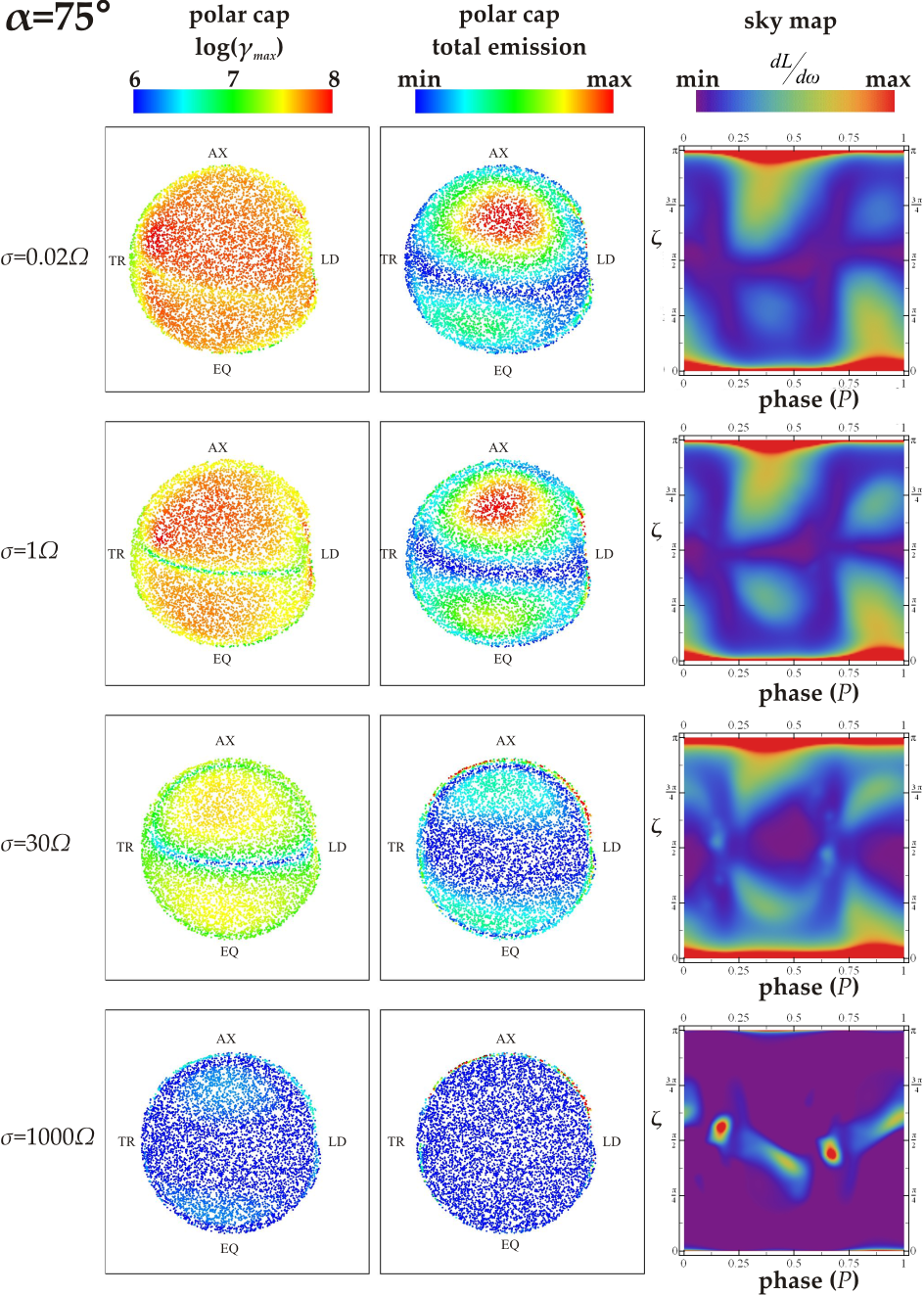
In Fig. 7 we show in color scale the polar cap maps of the $\log$ of the maximum value of $\gamma_{L}$ along each trajectory ($\gamma_{L_{\max}}$, left-hand column) and the total (along the entire trajectory) emission (middle column) for $\alpha=75^{\circ}$ and the indicated $\sigma$ values. We see that for low $\sigma$ models the particles can reach values up to $\gamma_{L_{\max}}\gtrsim 10^{8}$. These values are reached in the inner magnetosphere (well inside the LC) with their upper limiting values determined by the radiation reaction limit (curvature radiation energy loss rate equal to energy gain due to $E_{\parallel}$). The values of $\gamma_{L_{\max}}$ decrease with increasing $\sigma$ and for $\sigma=1000\Omega$ most of them drop below $10^{6}$ with only the highest ones reaching the value $\simeq 10^{6.5}$.

The total emission map (middle column) shows a similar pattern but it nevertheless differs since it is modulated by the $R_{\rm CR}$ values and the distribution of the $\gamma_{L}$ values all along the trajectories. The patterns shown in the left-hand and middle columns of Fig. 7 resemble that of the current density distribution on the polar cap (see Fig. 1) confirming, generally, that $E_{\parallel}$ is higher wherever the poloidal current is higher. However, as $\sigma$ increases and $E_{\parallel}$ decreases, $\gamma_{L}$ becomes sufficiently large to emit significant curvature radiation at increasingly larger distances. In these high $\sigma$ cases, the most efficiently radiating trajectories are those that see high $E_{\parallel}$ at large distances (beyond the LC). These trajectories are those reaching close to the equatorial current sheet near which we generally have high $E_{\parallel}$ (because the current density requirement in the FFE regime in this region is high). These trajectories originate near the edge of the polar cap (last open field lines) and that is why we observe (Fig. 7) in these regions, gradually, relatively higher $\gamma_{L_{\max}}$ and total emissions (than in the other regions). Nevertheless, Fig. 7 shows clearly that the total emission is not uniformly distributed over the region near the equatorial current sheet (i.e. the emission is not uniformly distributed all over the polar cap rim).

Figure 8.— The $\gamma$-ray light-curve atlas together with the corresponding sky-maps for $\sigma=0.02\Omega$. In each sky-map, for different inclination angles $\alpha$, gray horizontal lines are plotted at the $\zeta$ values for which the light-curves are displayed. In this case all the emission comes from the inner magnetosphere within the light-cylinder. The corresponding light curves are not very narrow.

As we mentioned above, for high $\sigma$ the values of $E_{\parallel}$ are small and consequently the particle energies and the corresponding $\gamma_{L}$ values are not efficient in producing significant emission in the inner magnetosphere (within the LC). However, the $\gamma_{L}$ values with which the particles reach the LC are not equal. The distribution of the $\gamma_{L}$ values on the LC depends on what $E_{\parallel}$ the particles encounter up to the LC. For small $E_{\parallel}$ (i.e. high $\sigma$) the $\gamma_{L}$ value depends mostly on the energy gain (first term in the right-hand side of Eq. 13) up to the LC (since the corresponding energy loss due to curvature radiation is small). This essentially means that the particles starting on the polar cap regions where the current reaches the stellar surface in a current sheet form (see Fig. 1) will have the highest $\gamma_{L}$ values at the LC because they encounter (amongst all polar cap particles) the highest $E_{\parallel}$ values within the LC. The non-uniformity of the $\gamma_{L}$ values on the LC affects the relative efficiency of the radiation beyond this point due to the $E_{\parallel}$ these particles see in the regions near the equatorial current sheet outside the LC. Higher $\gamma_{L}$ value on the LC means stronger emission beyond the LC near the equatorial current sheet.

The previous study provides the direction of the emitted photons (tangentially to the trajectories) and the corresponding bolometric emission ($\propto\gamma_{L}^{4}R_{\rm CR}^{-2}$) along each trajectory. This information allows us to construct $\gamma$-ray light curves by collecting all the photons in sky-maps taking into account time-delay effects. In the right-hand column of Fig. 7 we plot the sky-maps for $\alpha=75^{\circ}$ and for the indicated $\sigma$ values. Each sky-map depicts, in the indicated color scale, the emitted luminosity per solid angle ($dL/d\omega=dL/\sin(\zeta)d\zeta d\phi_{ph}$). The horizontal axis represents the phase of the pulsar rotation while the vertical axis represents the observer inclination angle $\zeta$. The zero phase is assigned to photons emitted close to the stellar surface on the $\boldsymbol{\mu}{\bf-\Omega}$ plane. Each observer sees a different light curve depending on its $\zeta$ value. The observed light curve is the horizontal cut of the sky-map at the observer’s $\zeta$ value.

The high emission we observe for low $\sigma$ values (Fig. 7, right-hand column for $\sigma=0.02\Omega$, $\sigma=1\Omega$) comes from lobes of points above the polar caps well within the LC. As $\sigma$ increases these lobes become smaller, making the emitting regions on the sky-maps narrower while gradually there appear additional components coming from regions near the equatorial current sheet. For very high $\sigma$ ($\gtrsim 300\Omega$) all the emission comes from specific regions near the equatorial current sheet (see bottom panel in middle-column of Fig. 7) and the corresponding emitting regions on sky-maps are narrow.

The sky-map pattern shown in Fig. 7 for $\sigma=1000\Omega$ is quite different than that corresponding to uniform emission in the entire equatorial current sheet. As we explained above, for very high $\sigma$ values, the trajectories that start from polar cap regions, where the current reaches in a current sheet form, radiate much more effectively beyond the LC. However, for the smaller $\alpha$ values ($\leq 45^{\circ}$) these regions on the polar cap are quite extended and so the corresponding sky-maps are very similar to those produced by uniform emission over the entire equatorial current sheet. In the bottom panel of right-hand column of Fig. 4 we see that emission is produced by the largest part of the equatorial current sheet (though still not totally uniform). On the other hand for larger $\alpha$ values ($>45^{\circ}$) the current sheet part reaching the polar cap is small; because of the limited extent of this region, whose particle trajectories provide all the radiation, the equatorial current sheet emission is far from uniform, something that affects the radiation pattern on the sky-map.

4.2. Comparison with Fermi Observations

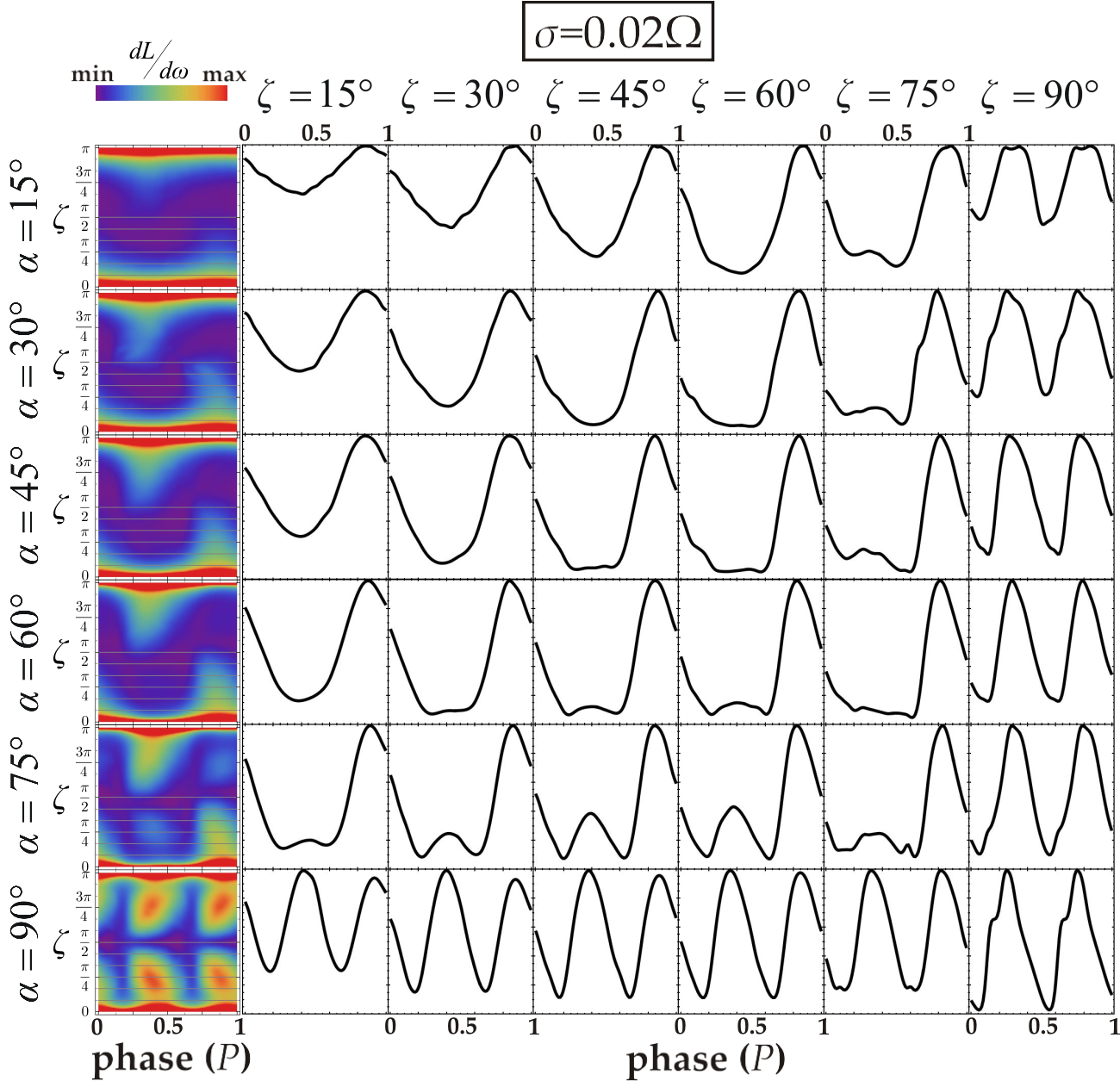
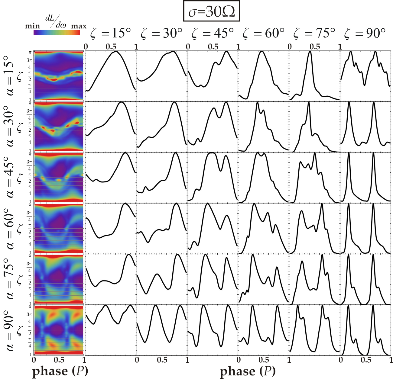
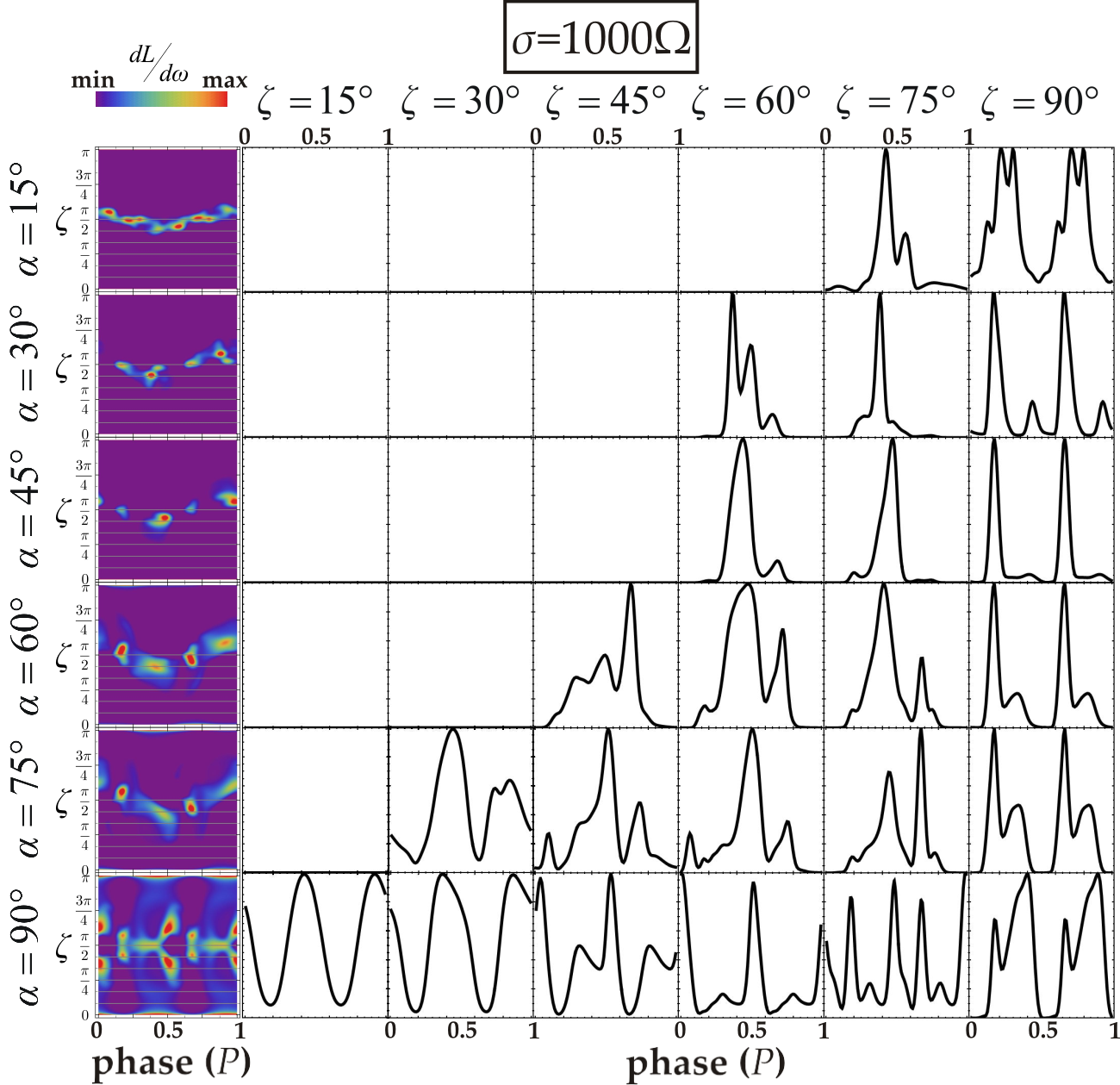
In Figs. 8, 9 and 10 we plot light-curve atlases for $\sigma=0.02\Omega,30\Omega$, and $1000\Omega$, respectively. Each atlas presents the light curves for the indicated inclination and observer angle ($\alpha,\zeta$) values. For $\sigma=0.02\Omega$ (Fig. 8) we see single and double peaked light-curves but the pulses seem to be rather wide. In general, the light curves become double peaked as we go towards high $\alpha$ and/or $\zeta$ values. For $\sigma=30\Omega$ (Fig. 9) there are cases (mostly near high $\zeta$ values) where the light-curves are quite narrow. However, there are cases where the light-curves are still wide and in some cases they look more complicated. This happens because for this level of $\sigma$ values there are different emitting components from both the inner (within the LC) and the outer (outside the LC) magnetosphere. When an observer is in a direction ($\zeta$ value) that sees both components the corresponding light-curve becomes more complex. For much higher $\sigma$ all the emission comes from the outer magnetosphere outside the LC in regions near the equatorial current sheet. Figure 10 shows that most of the light-curves, for $\sigma=1000\Omega$, are narrow. Moreover, in this case the observers of relatively small $\zeta$ values do not cross any significantly emitting region and so the corresponding part of the atlas is empty. ‘Significantly emitting’ in this case means that the maximum luminosity per unit solid angle for the specific $\zeta$ is larger than 2% of the corresponding maximum value of the entire sky-map. Below that value we don’t get clear and reliable information. In some of these cases it is also difficult to determine a clear primary and/or a secondary local maximum. Above that $\sigma$ value the light-curve shape saturates and remains almost the same.

Some of the light-curve shapes shown in Figs. 8-10 resemble those observed while others do not. However, in the vast majority of the observed pulsars we have no clue about either their inclination angle ($\alpha$) or our observer angle ($\zeta$) and so it is not easy to say whether a specific pulsar is described and up to what level by each model. Thus, we need a statistical comparison between the results provided by our models and the observational data. In this paper we are interested in checking the light-curve phenomenology, leaving for a forthcoming paper the study of the energetic part of the high energy emission.

Figure 9.— Same as in Fig. 8 but for $\sigma=30\Omega$. A significant part of the emission is produced in regions near the equatorial current sheet that has formed outside the light-cylinder. Some light-curves appear complex since in these cases the corresponding observer sees emission coming from different parts (inner and outer) of the magnetosphere.

Figure 10.— Same as in Figs. 8 and 9 but for $\sigma=1000\Omega$. All the emission is produced in regions near the equatorial current sheet outside the light-cylinder. However, the emissivity is not uniform in these regions due to the modulation of the parallel electric components remaining within the light-cylinder. Nonetheless, the light-curves are, in general, narrow. The empty panels in this atlas are for $\zeta$ values where no radiation is observed for the corresponding $\alpha$ values.

As we mention in the first section, a robust statistical result is the correlation of the $\gamma$-ray peak-separation $\Delta$ and the radio-lag $\delta$ between the $\gamma$-ray and radio emission. Figure 11 shows the $\delta$ vs $\Delta$ plot of the Second Fermi Pulsar Catalog (2PC) data (Abdo et al., 2013) together with the data of the dissipative models of the indicated $\sigma$ values assuming that the radio emission comes from a region near the magnetic pole on the pulsar surface. This assumption for the radio phase neglects phase shifts (that would increase $\delta$) due to aberration and retardation that result from emission at a significant altitude relative to $R_{\rm LC}$. In reality, the observed statistics in $\delta-\Delta$ diagram is expected to depend on the details of both the radio and $\gamma$-ray emitting models and on the possible population biases of the radio and $\gamma$-ray pulsars. Thus, for instance, the probability for radio photons to be observed is expected to be higher (lower) for low (high) $|\zeta-\alpha|$ values. However, in the current study we don’t incorporate any model of radio emission. Thus, all the radio-lag $\delta$ values presented below measure the time delays between $\gamma$-ray photons and radio photons which are thought to be emitted on the $(\boldsymbol{\mu},\boldsymbol{\Omega})$ plane near the stellar surface (assuming that the latter are always observed). We decided to plot and compare the 2PC data corresponding only to standard pulsars (and not the millisecond pulsars) since these objects (standard pulsars) present clearer and stronger indications that the radio emission is produced near the stellar surface. The 2PC data are plotted with black dots with error-bars while the model data are plotted with various shapes and colors. The color denotes the $\alpha$ value according to the indicated color scale (blue, low $\alpha$ to red, high $\alpha$) and the shape denotes the corresponding $\zeta$ value according to the indicated shape scale (full circle, low $\zeta$ to horizontal line, high $\zeta$). The $\Delta$ value is calculated as the phase difference (measured as a fraction of the stellar period, $P$) between the two highest local maxima. We note that any local maximum lower than $0.05$ of the value of the highest (first) maximum is not counted as a local maximum and the corresponding light curve is considered to have only one peak. The $\delta$ value is derived as the phase of the first peak of the $\gamma$-ray peak (assuming $0$ to be the phase emitted at the magnetic pole on the stellar surface). We note that the phase $\phi_{ph}$ of a photon emitted at a point $A$ along the trajectory of a particle (integrated in the inertial frame) is given by

$$\phi_{ph}=\left(\Omega t_{A}-\phi_{\mathbf{v_{A}}}-\frac{\mathbf{r_{A}}\cdot\mathbf{v_{A}}}{v_{A}}\frac{1}{R_{\rm LC}}\right)\negthickspace\negthickspace\negthickspace\mod 2\pi$$ (15)

where $t_{A}$ is the integration time corresponding to the point $A$ (assuming that the integration starts at the stellar surface), $\mathbf{v_{A}},\mathbf{r_{A}}$ are the particle velocity and position vectors at $A$, and $\phi_{\mathbf{v_{A}}}$ is the azimuth angle of the velocity $\mathbf{v_{A}}$ with respect to the magnetic axis at $t=0$ oriented according to $\mathbf{\Omega}$. The last term in Eq. (15) formulates the light travel time delay.

For low $\sigma$ values ($\sigma=0.02\Omega$ and $\sigma=1\Omega$) we have run 6 models (every $15^{\circ}$, $\alpha=15^{\circ},~{}30^{\circ},\ldots,90^{\circ}$) and we have calculated the $(\delta,~{}\Delta)$ values for 6 $\zeta$ values $(\zeta=15^{\circ},~{}30^{\circ},\ldots,90^{\circ})$ while for $\sigma>1\Omega$ we have run 17 models (every $5^{\circ}$, $\alpha=10^{\circ},~{}15^{\circ},20^{\circ},\ldots,90^{\circ}$) and we have calculated the $(\delta,~{}\Delta)$ values for 17 $\zeta$ values ($\zeta=10^{\circ},~{}15^{\circ},20^{\circ},\ldots,90^{\circ}$). This means that the plots of Fig. 11 for $\sigma\leq 1\Omega$ may have up to 36 model data points while those for $\sigma>1\Omega$ may have up to 289 model data points.

Figure 11.— Diagram showing radio-lag $\delta$ vs the $\gamma$-ray peak-separation $\Delta$ for the models (color elliptical points) corresponding to the indicated $\sigma$ values. In each panel, the black points (with error-bars) correspond to standard pulsars (and not the millisecond ones) observed by Fermi (2PC). The color and the shape of the model points denote the $\alpha$ and $\zeta$ values, respectively as indicated in the figure. We note that for $\sigma=0.02\Omega$ and $\sigma=1\Omega$ we have considered a smaller number of $\alpha$ and $\zeta$ values than those for the higher $\sigma$ values (see text for more details). The low $\sigma$ models have the highest radio-lag values among all the models. In this case all the model points lie in regions absent of observed points. As $\sigma$ increases the model points move toward smaller radio-lag values (closer to the observed values). For very high $\sigma$ values many model points lie near the observed ones while there are still points, corresponding mostly to high $\alpha$ values, that lie in regions not covered by the observed ones.

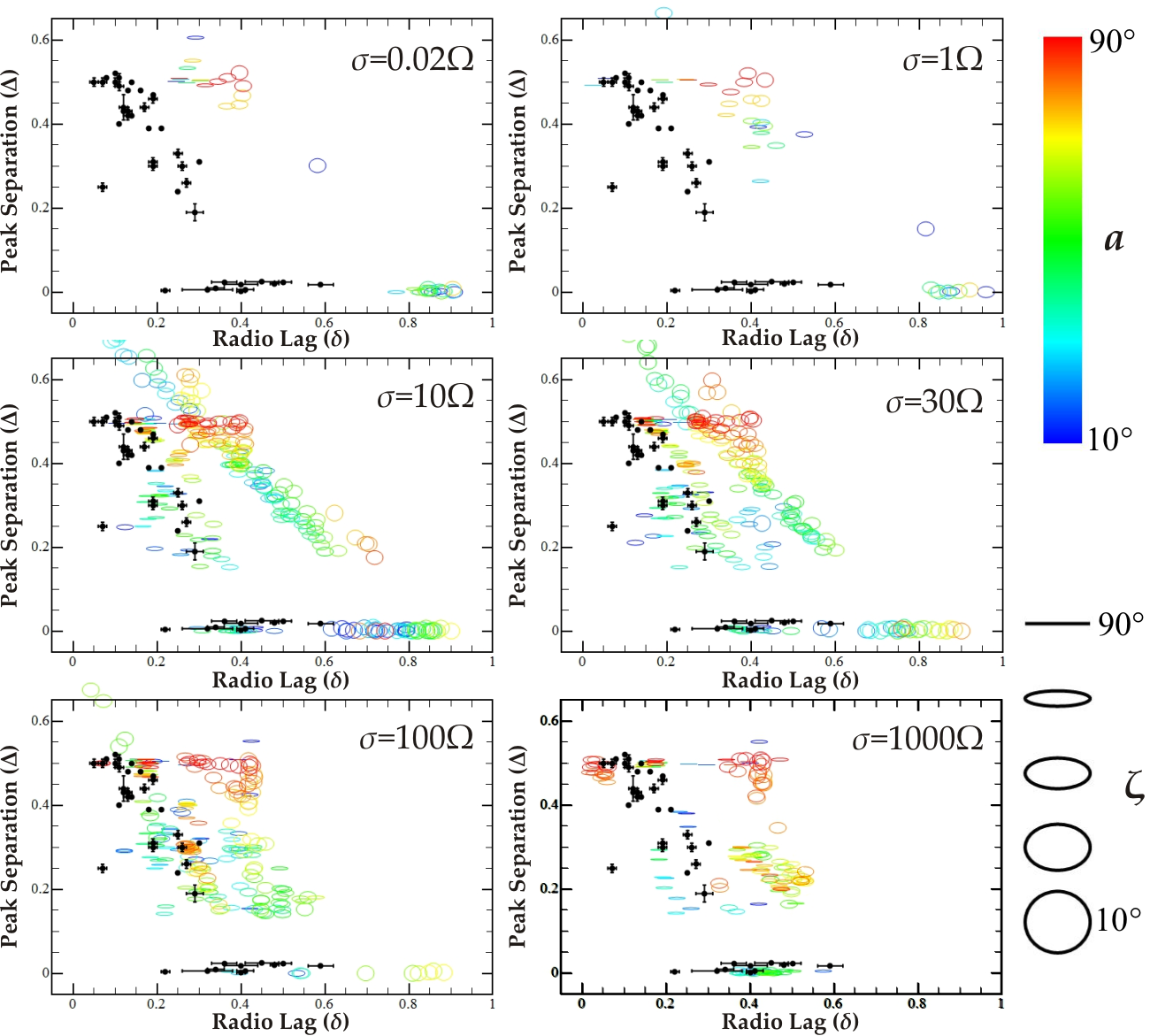
The values of ($\delta,~{}\Delta$) can be determined from the shapes of the computed model pulses. However, because this procedure is time consuming and possibly biased, we have developed an algorithm that takes into account most of the human-eye criteria employed in the determination of ($\delta,~{}\Delta$) values. This allowed an automatic, unbiased and fast computation of the ($\delta,~{}\Delta$) values directly from the corresponding sky-map data. Such an automatic calculation may lead to some errors (false points). However, we expect the number of these false points to be small since we checked more than a hundred light-curves of various types and in more than 90% of the cases the results were in total agreement with those derived by simple eye examination. These false points come from non-standard light-curves (more than two clear peaks from more than one radiating components) and do not affect the underlined statistics.

Figure 12.— Histograms of the fraction of observed points (gray color) and model points (light green color) at a given radio-lag $\delta$, for the indicated $\sigma$ values, along the radio-lag $(\delta)$ axis of Fig. 11. The dark green color indicates coexistence of two histograms. The histograms for the models depend on the results presented in Fig. 11. However, the results of Fig. 11 correspond to uniform distribution functions for $\alpha$ and $\zeta$ while these histograms have been calculated assuming a uniform distribution function for $\alpha$ and spherically uniform distribution function for $\zeta$. We see that low $\sigma$ models do not have good agreement with the observations. Higher $\sigma$ models cover the entire range of the observed $\delta$ values but the distributions differ from the observed ones.

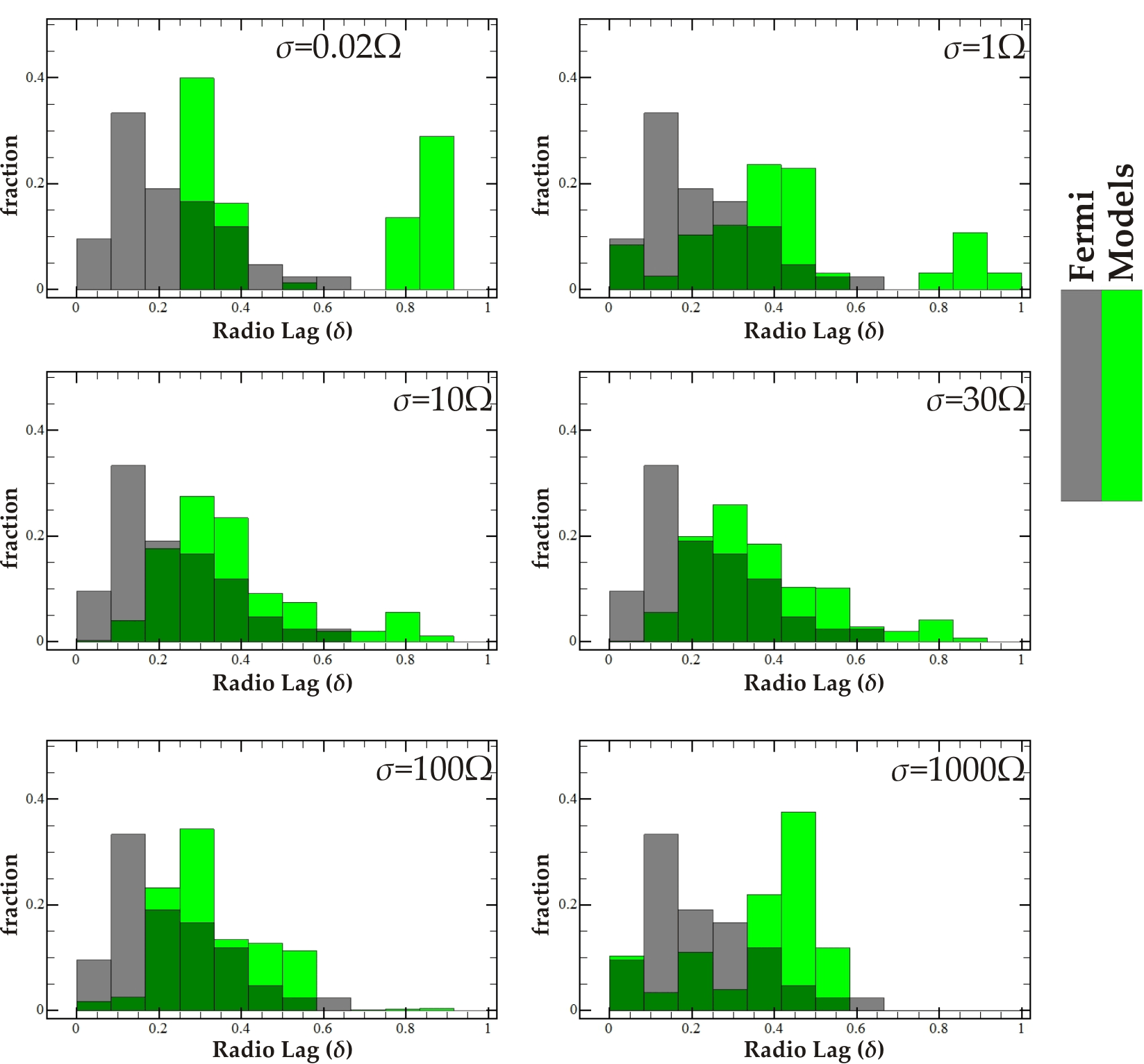
In Figs. 12 and 13 we plot the projected fraction distributions (in green histograms) of the models shown in Fig. 11 along the $\delta$ and $\Delta$ axes, respectively, keeping the axis orientation of Fig. 11. Each panel shows also the fraction distributions of the observed points (in gray histograms). We note that the model statistics shown in Figs. 11-13 depend not only on the $\sigma$ value but also on the probability distribution functions of $\alpha,~{}(F_{\alpha})$ and $\zeta,~{}(F_{\zeta})$. Apparently, the allocation of model points in Fig. 11 corresponds to uniform distributions for $\alpha$ and $\zeta$. For $\alpha$ the intrinsic probability distribution function $F_{\alpha}$ is unknown but for $F_{\zeta}$ there is no reason why this would be different from a spherically uniform $F_{\zeta}\propto\sin(\zeta)$. Thus, the histograms in Figs. 12, 13 are modified with respect to the data of Fig. 11 so that they are in compliance with a uniform distribution in $\alpha,~{}F_{\alpha}(\alpha)\propto 2/\pi$ and spherically uniform distribution in $\zeta,~{}F_{\zeta}(\zeta)\propto\sin(\zeta)$.

Figure 13.— Same as in Fig. 12 but for $\Delta$ axis. Note that we have kept the axis orientation shown in Fig. 11.

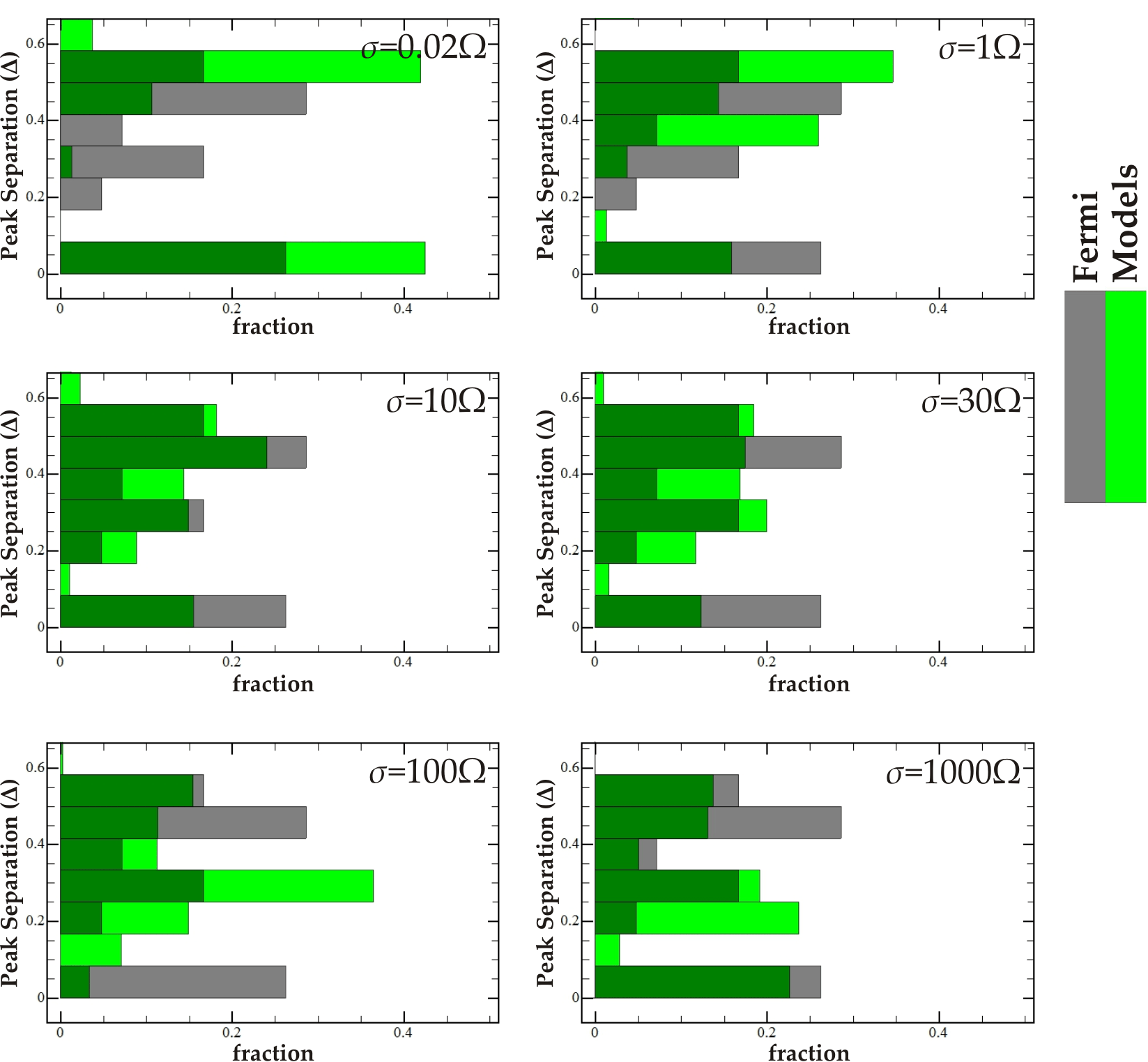
Figures 11-13 show that for $\sigma=0.02\Omega$ there are mostly two groups of points (one near $\Delta=0$ and one near $\Delta=0.5$) that have much higher $\delta$ values than the observed ones. The group near $\Delta=0.5$ consists in general of points coming from higher $\alpha$ values than those we see in the group near $\Delta=0$. For $\sigma=1\Omega$ we still see the same two groups of points but now some of the points of the group near $\Delta=0.5$ have moved either towards smaller $\delta$ values or smaller $\Delta$ values trying to fill the gap between the two groups. For a higher $\sigma$ ($\sigma=10\Omega$) many model points have moved to even smaller $\delta$ and $\Delta$ values overlapping the region covered by the observed points while many model points lie along a diagonal line, parallel to the arrangement of the observed points, at higher $\delta$ values. As $\sigma$ increases, more model points lie in the observed region while the points remaining along the diagonal approach slightly the observed region ($\sigma=30\Omega$) and become more dispersed ($\sigma=100\Omega$). Above this $\sigma$ value the total number of model points decreases since for some $\zeta$ values the pulsars become invisible (see Fig. 10). This effect affects the histograms by increasing the relative fractions at higher $\delta$ and lower $\Delta$. Nonetheless, for higher $\sigma$ the model point distributions saturate consisting always of points that lie in the observed region and points that clearly lie in regions absent of observed points. We note that the latter model points correspond mainly to higher $\alpha$ values.

Figure 14.— Same as Fig. 15 but for the CSUE models. We see a variety of light-curve shapes similar to those observed by Fermi.

5. Successful Models

The results presented in the previous section, provide the basic properties and trends of the radiation patterns in dissipative models of uniform $\sigma$ in the open field line region. This study showed that the low $\sigma$ models are consistent with inner magnetosphere emission (within the LC) while the high $\sigma$ models (near-FFE) are consistent with outer magnetosphere emission in regions near the equatorial current sheet outside the LC. Moreover, the detailed comparison with the observed phenomenology seems to rule out (under the assumption that the radio emission is produced near the magnetic poles) the very low $\sigma$ models since these models appear to have systematically larger radio-lags than the observed ones contrary to what the application of the theoretical accelerating models (Outer-Gap, hereafter, OG; Slot-Gap, hereafter, SG; Cheng et al., 1986; Romani & Yadigaroglu, 1995; Muslimov & Harding, 2004) on dissipative magnetosphere solutions has shown (Bai & Spitkovsky, 2010; Harding et al., 2011; Kalapotharakos et al., 2012b). In fact, the theoretical accelerating models under the geometry of near-vacuum solutions indicate smaller radio-lags than those we get under the geometry of near-FFE solutions. However, the theoretical acceleration models in this case (near-vacuum solutions) assume the presence of significant $E_{\parallel}$ in regions where they do not actually exist. On the other hand, the high $\sigma$ models (near-FFE) signify the importance of the regions near the equatorial current sheet and are clearly closer to observations. They show a set of light curves that fit the observations while another set has larger radio-lags than those observed. This inconsistency leaves open questions on whether the uniform $\sigma$ models are able to reproduce the observed $\gamma$-ray light-curve phenomenology. Nevertheless, as we will see, the study above reveals a way to find the successful models.

Up to now we have assumed a uniform $\sigma$ distribution in the open field regions (the closed field line region has always high $\sigma$) and that the radio emission is produced near the magnetic poles. The uniform $\sigma$ is the simplest and most unbiased approach since it gives a uniform level of screening of $E_{\parallel}$ everywhere. This means, especially for the high $\sigma$ (near-FFE) solutions, that the screening of the $E_{\parallel}$ is more difficult wherever the required FFE $(\boldsymbol{\nabla}\times\mathbf{B})_{\parallel_{\text{FFE}}}$ is higher. We note that this is, in general, valid for all the current density $\mathbf{J}$ prescriptions tested in this study.

Figure 15.— The $\delta$-$\Delta$ diagram for the Current Sheet Uniform Emission (CSUE) model together with the corresponding histograms along $\delta$ (top) and $\Delta$ (right) axes. Even though these models are in a better agreement with observations than the dissipative models shown in Figs. 11-13 they still present a systematic trend of model radio-lag $(\delta)$ values that are higher than those observed. In each histogram panel we have indicated the corresponding $g$ values derived by relation (16) for uniform $\alpha$ distribution (all $w_{\alpha_{i}}$ are equal).

Figure 16.— A simplified picture that describes the structure of the models successfully reproducing the observed $\gamma$-ray light-curve phenomenology. The blue sphere and the green cylindrical surface represents the pulsar and the light-cylinder, respectively. This type of model assumes a FFE regime Inside the light-cylinder and Dissipative Outside (FIDO).

Assuming that the flow across the polar cap is not highly non-uniform the discrepancy between the model data and the Fermi data, present even for the highest $\sigma$ values shown in Figs. 11-13, could indicate primarily two things:
Either

1. that the radio emission is not produced near the magnetic poles

or

1. that the adopted $\sigma$ distribution and/or the adopted Ohm’s law are not the correct ones.

Case (a) is in contradiction with a widely observed phenomenology (e.g. Rankin, 1983) and we will not consider this option in this paper. The second case (b) seems reasonable and it should be related to the detailed properties of the underlined microphysics of pair creation. Nonetheless, the analysis presented in Section 4 indicates that the non-uniform “lighting” of different parts of regions near the equatorial current sheet may produce different radiation patterns on the sky-maps. Contopoulos & Kalapotharakos (2010), Bai & Spitkovsky (2010), Pétri (2011) and Arka & Dubus (2013) have already presented $\gamma$-ray light-curves and studied some of their phenomenological properties assuming either constant emission or constant $\gamma_{L}$ values on the equatorial current sheet. However, only Contopoulos & Kalapotharakos (2010) attempted a coarse comparison with the observed phenomenology in the First Fermi Pulsar Catalog (1PC).

Figure 17.— Same as Fig. 15 but for the FIDO models. We see that these models are in a very good agreement with the observations. The indicated $g$ values are considerably smaller than those of CUSE models (Fig. 15).

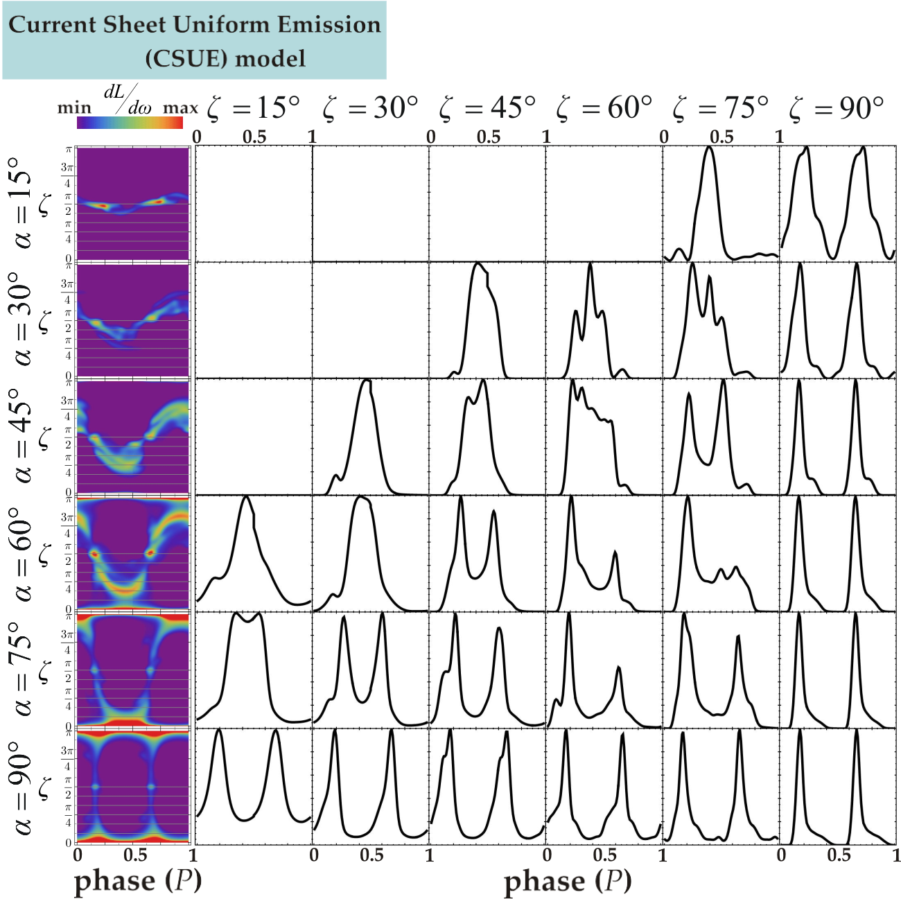
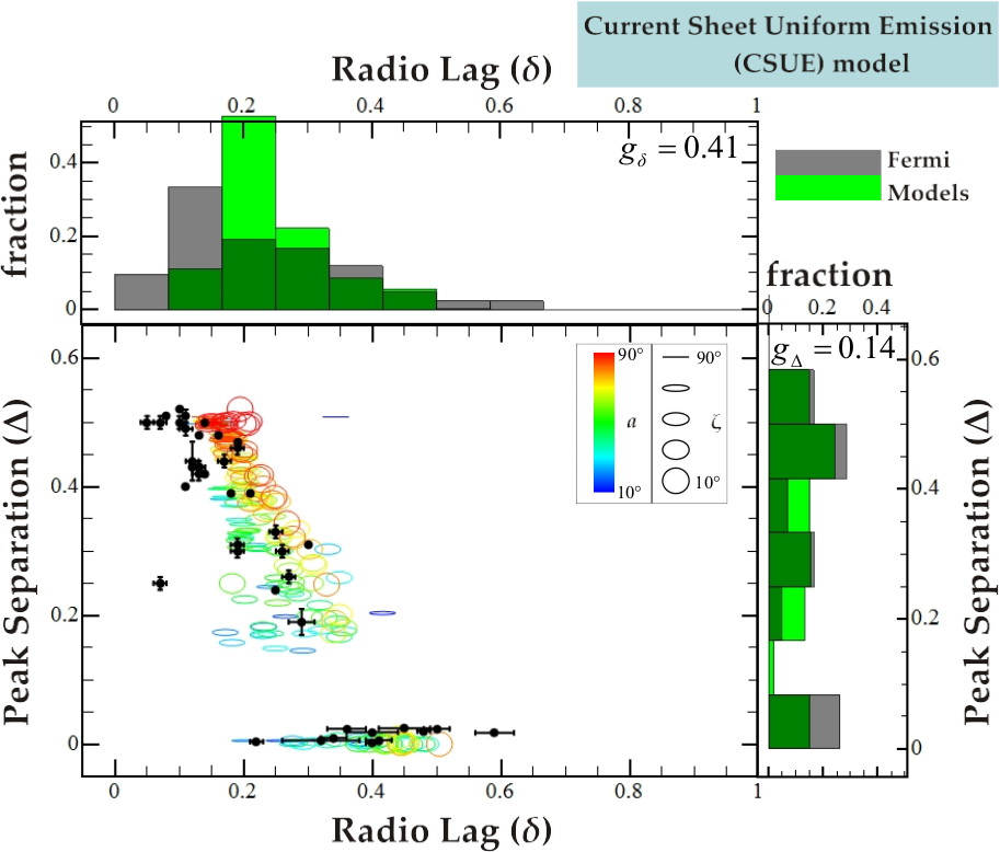
We first make, for comparison, a detailed statistical analysis of the $\delta-\Delta$ relation for the dissipative models, assuming uniform emissivity everywhere on the equatorial current sheet of the FFE solutions. For this we assumed that all the particles start from the outer parts of both polar caps. More specifically, using the Open Volume radial, $r_{\rm ovc}$, and azimuthal, $\phi_{\rm ovc}$, Coordinates (OVCs) (Dyks & Harding, 2004) defined inside the open volume of each FFE solution, we assume that particles originate in a uniform distribution within the thin layer between $r_{\rm ovc}=0.95-1$ of the corresponding polar cap radius. We integrate the trajectories of these particles up to $2.5R_{\rm LC}$ assuming constant emissivity along their length. Figure 14 shows the sky-maps and the corresponding light curve atlas. These results are very similar to the Separatrix Layer (SL) model in Bai & Spitkovsky (2010). Actually, our sky-maps seem a little more complex than those of Bai & Spitkovsky (2010) mostly because we have considered uniform particle flux over the entire part of the polar cap with $r_{\rm ovc}=0.95-1$ instead of a flux from a narrow zone around $r_{\rm ovc}=0.90$ or $0.95$. In Fig. 15 we present the ($\delta,\Delta$) statistics together with the corresponding histograms along $\delta$ and $\Delta$ axes, for the FFE (or near-FFE) models assuming uniform emission (up to $2.5R_{\text{LC}}$) on the equatorial current sheet. All these panels include the 2PC data for comparison. Figure 15 shows that the Current Sheet Uniform Emission model (hereafter, CSUE) is in better agreement with the observations than the series of dissipative models presented in Figs. 11-13. Nonetheless, it is apparent that there is a strong trend toward higher radio-lag values $(\delta)$ compared to those observed. This difference becomes clearer in the distribution along the $\delta$ axis.

Figure 18.— Same as Fig. 8 but for the FIDO models. The adopted conductivity value outside the light-cylinder is $30\Omega$. The emission comes from regions near the equatorial current sheet. The emissivity distribution is affected by the local physical properties and is not symmetric around the equatorial current sheet. This adjusts the corresponding radio-lag values toward the observed values. Moreover, there is no emission for low $\zeta$ and high $\alpha$ values. We see also narrow, well-defined $\gamma$-ray light-curves with low off-peak emission.

Figure 19.— (a) Same as the panels in the middle column of Fig. 7 but for the $\alpha=75^{\circ}$ FIDO model. We see that the high emission is produced mostly from particles that originate at the leading edge of the polar cap. (b) Same as the panels of the right-hand column of Fig. 4 but for the $\alpha=75^{\circ}$ FIDO model. We see that most of the emission is produced in regions near the equatorial current sheet around the rotational equator.

On the one hand, the high $\sigma$ models presented in Figs. 11-13 fail because the emission from a region near the equatorial current sheet is modulated by the distribution of $E_{\parallel}$ within the LC. On the other hand, when we assume constant emission, as in CSUE models, we still are not able to reproduce the observed statistics. However, both cases show that the emission from the outer magnetosphere emerging from physical properties of the near-FFE solutions in regions near the equatorial current sheet is important.

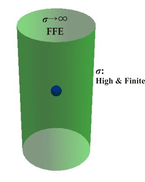
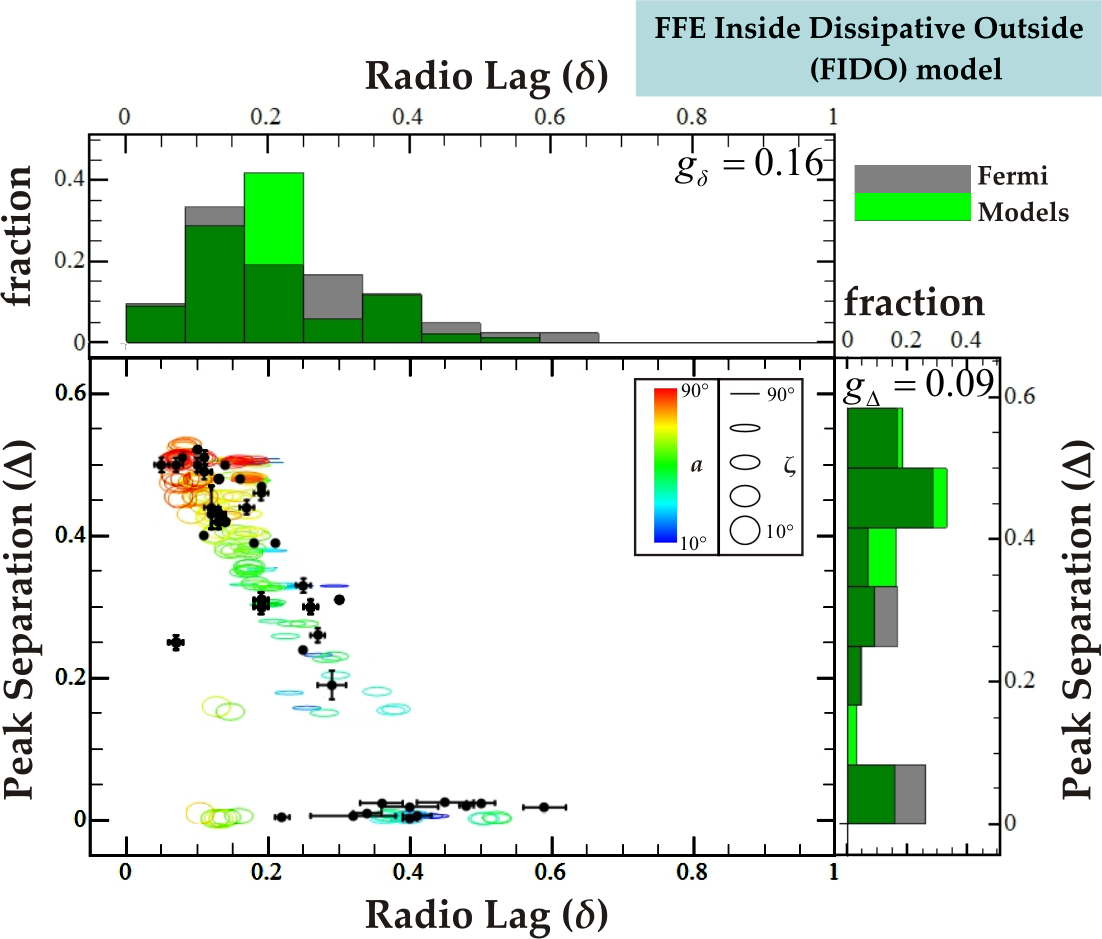
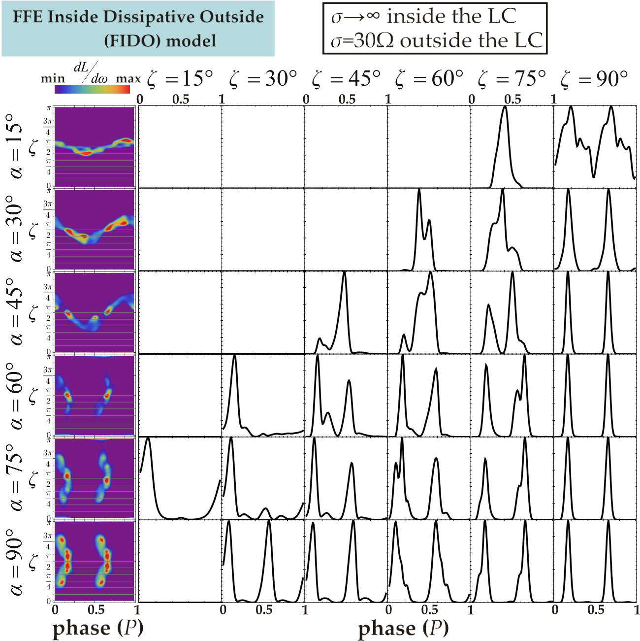
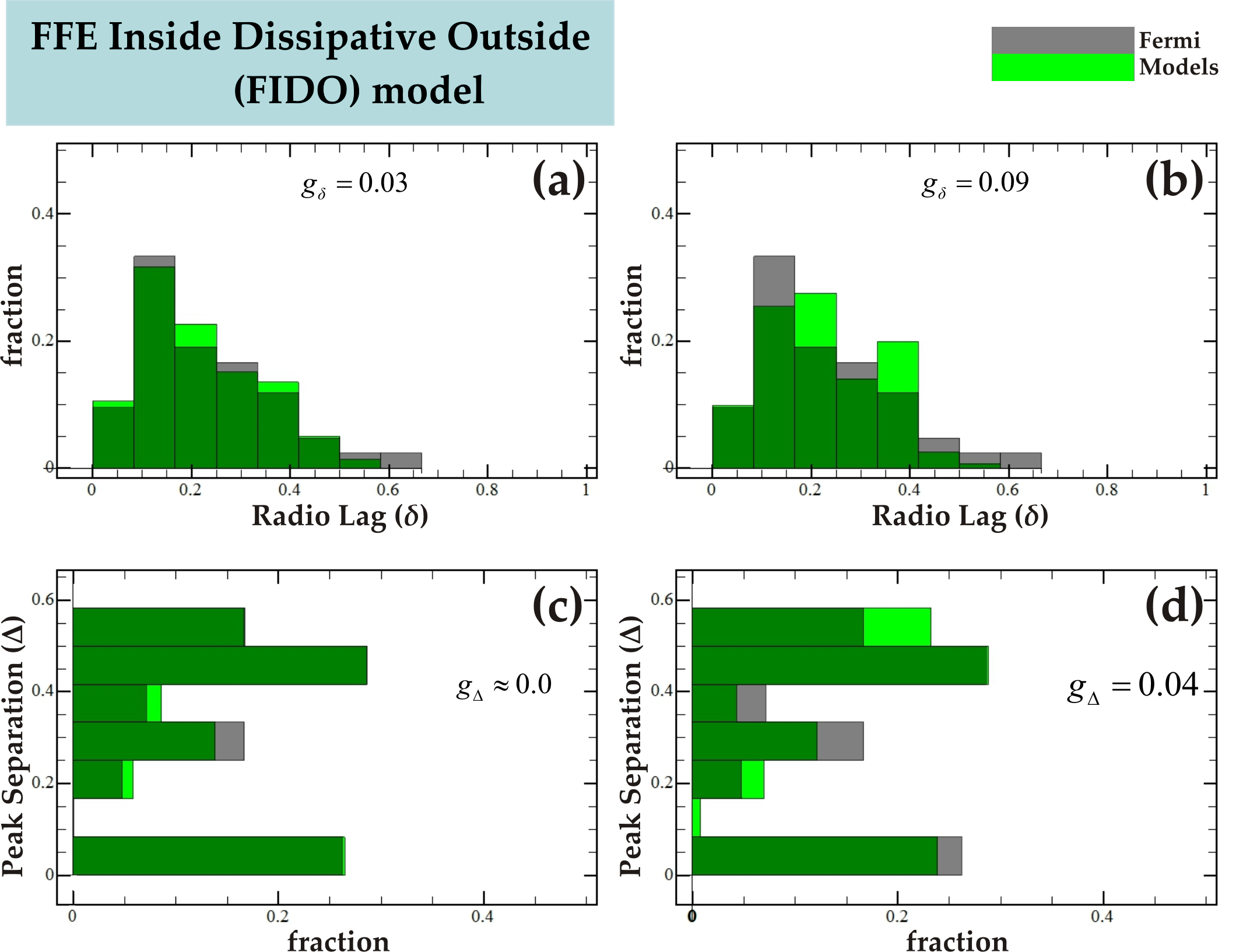
We consider an alternative simple model that retains the emission near the equatorial current sheet and the physical properties of the dissipative solutions but avoids its modulation from the inner magnetosphere. We assume a hybrid FFE-Inside & Dissipative-Outside model (hereafter, FIDO) that has an FFE regime $(\sigma\rightarrow\infty)$ within the LC and high (but finite) $\sigma$ outside the LC (see Fig. 16). In this model, the inner magnetosphere no longer affects the radiation patterns while the finite $\sigma$ in the outer magnetosphere allows the regions near the equatorial current sheet to determine the radiation patterns based only on the local physical properties. Figure 17 shows the $\delta-\Delta$ distribution corresponding to these hybrid models for $\sigma=30\Omega$ outside the LC together with the 2PC data. Remarkably, these models are by far the best in reproducing the observed 2PC statistics. The high energy radiation in this case is produced in regions near the equatorial current sheet but the corresponding radiation patterns depend exclusively on the local physical properties with no contribution from inside the LC. This affects the radiation patterns of the models, with those having the higher inclination angles $(\alpha>45^{\circ})$ being the most affected.

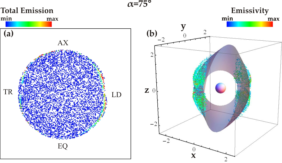
Figure 18 presents the light-curve atlas of FIDO models. We see narrow and well defined light-curves that resemble those observed by Fermi. For low $\alpha$ values $(\alpha\leq 45^{\circ})$ the emission comes from regions near the entire equatorial current sheet while for higher $\alpha$ values $(\alpha>45^{\circ})$, where the equatorial current sheet extends to lower colatitudes, the emission comes from regions near the equatorial current sheet that are closer to the rotational equator. This effect eliminates the corresponding emission at low $\zeta$ values. In Fig. 19a we map, in the indicated color scale, the total luminosity on the polar cap for $\alpha=75^{\circ}$ (similar to the middle column of Fig. 7). We see that the high emission trajectories lie near the edge of the polar cap. This clearly indicates that all the emission is produced in regions near the current sheet beyond the LC. However, the emission is not uniform all along the polar cap edge. We observe stronger emission from the leading edge of the polar cap and from parts that are closer to the rotational axis. In Fig. 19b we plot, in the corotating frame, the points that trace the comoving (prescribed by the particle flux) volume that contribute to the highest 95% of the total emission in the FIDO model of $\alpha=75^{\circ}$. We see that most of the emission comes from a region near the equatorial current sheet that has $\theta>45^{\circ}$ (where $\theta$ is the spherical polar angle) towards the rotational equator. These regions have high $E_{\parallel}$ and the particles that travel through them reach higher $\gamma_{L}$ values.

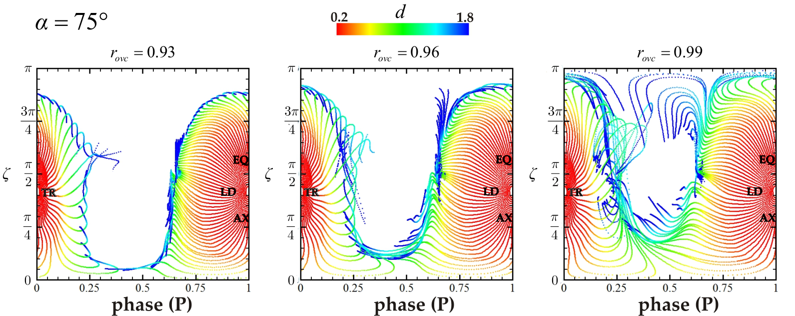
The sky-map emission pattern depends, in general, on (a) the distribution of the initial conditions ($r_{\rm ovc},\phi_{\rm ovc}$) of the highly emitting trajectories on the polar cap and (b) the altitude (distance) at which these trajectories emit. Bai & Spitkovsky (2010) have already presented the projections of particle trajectories on the sky-map based on the FFE geometry. Assuming constant and uniform emission along all the trajectories they concluded that the emitting patterns that match better the shapes of the observed $\gamma$-ray light curves are those that originate close to a ring corresponding to $r_{\rm ovc}=0.90$ or $r_{\rm ovc}=0.95$ (for each $\phi_{\rm ovc}$ the edge of the polar cap has $r_{\rm ovc}=1$). They noticed also that, in this case (FFE), the formation of the caustics is the result of the Sky Map Stagnation (SMS) effect which means that the strong emission in sky-maps is not due to the coincidence that emission from different trajectories congregates on the same point on the sky-map, but the emission from different points of a single trajectory arrives simultaneously, piling up on the same region of the sky-map. However, they noticed (and we confirm) that this effect is less prominent the lower the emission altitude is and the higher the $r_{\rm ovc}$ is. Nevertheless, their results (see fig. 6 and fig. 8 in Bai & Spitkovsky, 2010) indicate that high intensity regions on sky-maps can be produced by the concurrent contribution from different trajectories (especially for $r_{\rm ovc}\rightarrow 1$). In our case, instead of setting the $r_{ovc}$ limits of the emitting trajectories artificially, we allow the distribution of $E_{\parallel}$ from the model to determine the emitting geometry. In reality, the emissivity distribution among and along the trajectories is what will determine the emission pattern on sky-maps. The geometric properties and the effectiveness of the SMS phenomenon of the highly emitting trajectories will modulate the sky-map emission patterns accordingly.

In Fig. 20 we plot the sky-map projections of the trajectories originating from one (north) polar cap for the indicated $r_{\rm ovc}$ values (for the entire range of the $\phi_{\rm ovc}$ values). The color along the trajectory projections represents the distance $d$ traveled along each trajectory according to the indicated color scale. These results confirm the general picture presented by Bai & Spitkovsky (2010). We see that the SMS effect becomes stronger (i.e. shorter blue segments) as the $r_{\rm ovc}$ decreases. Figure 19a and the bottom middle panel of Fig. 7 show which trajectories presented in Fig. 20 are the ones that shine brightest producing the corresponding emission patterns on sky-maps.

The main differences that make FIDO models more effective in reproducing the $\delta-\Delta$ correlation than CSUE models are:

1. In FIDO models the emission is non-uniform along the equatorial current sheet in a way that emission at small $\zeta$ is negligible because the regions, near the equatorial current sheet, producing radiation for small $\zeta$ have small $E_{\parallel}$ for high $\sigma$ and consequently the particles in these regions have low and inefficient $\gamma_{L}$ values. This effect removes some points of higher $\delta$ values from the $(\delta-\Delta)$ diagram.

2. In FIDO models the emission is asymmetric across the equatorial current sheet. The higher emission (i.e. higher $E_{\parallel}$) originates from the leading edge of the polar cap rim. These trajectories have smaller $\delta$ values that push some of the points of $(\delta-\Delta)$ diagram to left (smaller values of $\delta$).

Figure 20.— Trajectory projections on the sky-map for $\alpha=75^{\circ}$. Each panel shows trajectories that originate from one (north) polar cap at the indicated $r_{ovc}$ values. The color along the trajectory projections illustrates the traveled distance $d$. Which trajectories emit and at what distance is what determines the emission pattern on the sky-maps.

The non-uniform and asymmetry effects were also present in the dissipative models of uniform (in the open field line region) $\sigma$ presented in Figs. 4-13. In the middle column of Fig. 7 we see that the total emission near the edge of the polar cap is not equal in diametrically opposed points. However, in that case these effects were modulated by the $E_{\parallel}$ of the inner magnetosphere and produced different emission patterns.

We have already mentioned that the statistical comparison between the models (CSUE and FIDO) and the 2PC observations presented in Fig. 15 and Fig. 17 depends on the unknown intrinsic probability distribution function of $\alpha$ $(F_{\alpha})$ and on the probability for the radio and $\gamma$-ray pulses to be observed together for the different $\alpha$ and $\zeta$ combinations. However, the determination of this last probability requires a detailed prescription for the radio emission as well, something that goes beyond the scope of this paper. Nonetheless, the determination of the $F_{\alpha}(\alpha)$ that minimizes the statistical differences between the models and the 2PC data on the $(\delta-\Delta)$ diagram is challenging. Thus, below we do this exercise and determine the $F_{\alpha}(\alpha)$ functions for the CSUE and FIDO models that fit best the data taking into account all the points plotted in Figs. 15 and 17.

The distribution on the $(\delta-\Delta)$ plane is 2D and so any 2D statistical comparison technique (e.g. Kolmogorov-Smirnov) is unreliable due to the relatively small number of observational points. Instead, we decided to find the relative weights for each $\alpha$ value that minimize the differences between the model-observation distributions, independently along the $\delta$ and $\Delta$ axis. In particular, we derived the values of $w_{\alpha_{i}}:(\alpha_{i}=10^{\circ},~{}15^{\circ}\ldots 90^{\circ})$ that minimize the

$$g_{\delta,~{}\Delta}(w_{\alpha_{i}})=\sum_{j=1}^{N_{b}}\frac{\left(\sum_{i=1}^{N_{\alpha}}w_{\alpha_{i}}P_{\alpha_{i}}^{j}-P_{O}^{j}\right)^{2}}{\sum_{i=1}^{N_{\alpha}}w_{\alpha_{i}}P_{\alpha_{i}}^{j}+P_{O}^{j}}$$ (16)

under the requirements $w_{\alpha_{i}}\geq 0:i=1\ldots N_{\alpha}$ and $\sum_{i=1}^{N_{\alpha}}w_{\alpha_{i}}=1$. In Eq. (16) $N_{b}$ is the number of bins we consider for the distributions along the $\delta$ and $\Delta$ axis. The quantity $P_{O}^{j}$ expresses the observable probability for the $j^{\rm th}$ bin while the quantity $P_{\alpha_{i}}^{j}$ expresses the probability of models with $\alpha=\alpha_{i}$ to be in the $j^{\rm th}$ bin. Finally $N_{\alpha}$ is the total number of different $\alpha$. The expression (16) is minimized using Interior Point method as this is implemented in Mathematica (Wolfram Research, Inc., 2010). We note that the $g_{\delta}$ and $g_{\Delta}$ values are not compared directly to each other since they refer to a different number of bins $(N_{b})$ along $\delta$ and $\Delta$ axis.

Figure 21.— The CSUE model fraction histograms (together with the observed ones) for the optimum $\alpha$ distributions. (a), (c) The model histograms along $\delta$ and $\Delta$ axes for the (different) $\alpha$ distributions that minimize the corresponding $g,~{}(g_{\delta},~{}g_{\Delta})$ values (Eq. 16), respectively. (b), (d) The model histograms along $\delta$ and $\Delta$ axes, respectively, for the $\alpha$ distribution that is the mean of the $\alpha$ distributions that independently minimize the $(g_{\delta},~{}g_{\Delta})$ values in (a), (c). In (a), (c) we see an improved performance for the CSUE models (with respect to Fig. 15)) even though they are still unable to reproduce the low radio-lag values. When the corresponding optimum $\alpha$ distributions are combined (b), (d) there is poorer agreement (especially along the $\Delta$ axis), indicating that the optimum $\alpha$ distributions adopted in (a) and (c) are not very similar.

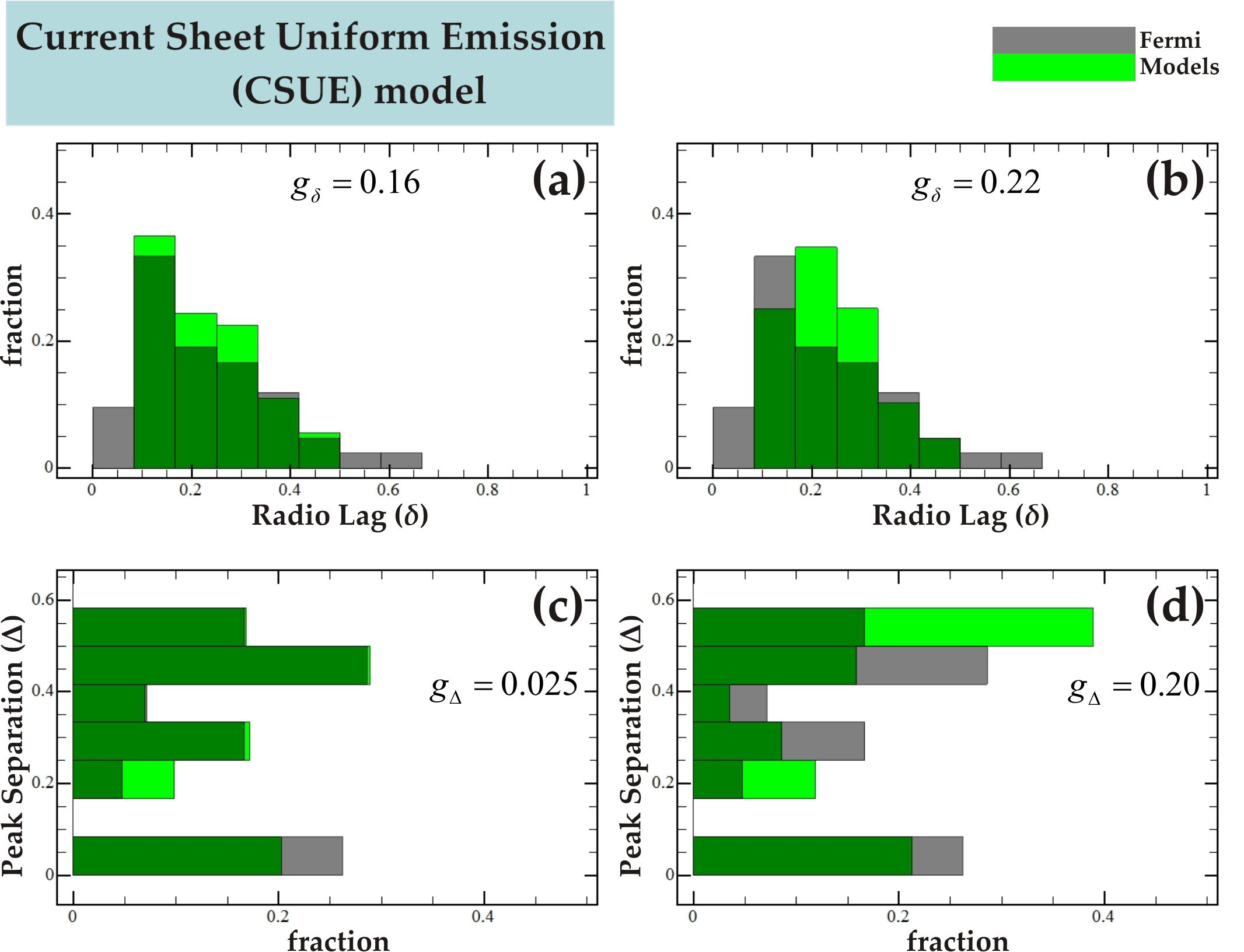
In Figs. 15, 17 we have indicated the $g$ values corresponding to uniform $\alpha$ distributions (all $w_{\alpha_{i}}$ are equal). We see that FIDO models have $g$ values that are considerably smaller than the (CSUE) models. This confirms our previous conclusions that the FIDO models fit the observational data quantitatively better than the CSUE models, under the assumption of uniform $\alpha$ distribution.

We calculated the $w_{\alpha_{i}}$ that minimize the $g(w_{\alpha_{i}})$ corresponding independently to the distributions along $\delta$ and $\Delta$ axes for both CSUE and FIDO models. In the top and bottom panels of the left-hand column of Fig. 21 we plot the optimized CSUE model distributions along $\delta$ and $\Delta$ axes, respectively. We see that each of these distributions are much closer to the observed distributions than those shown in Fig. 15 even though the lowest observed $\delta$ values cannot be reproduced. The corresponding $g(w_{\alpha_{i}})$ values are indicated on each panel of Fig. 21. However, the $w_{\alpha_{i}}$ sets that minimize the distributions along $\delta$ and $\Delta$ axes (Fig. 21a, c) have considerable differences. In order to compromise these differences we considered a common $(w_{\alpha_{i}})$ set that contains the average values of the two independent original $(w_{\alpha_{i}})$ sets. The distributions and the new $g(w_{\alpha_{i}})$ values corresponding to these average $(w_{\alpha_{i}})$ values are shown in the right-hand panels of Fig. 21. We see that the new distributions also differ considerably from the observed ones. This appreciable degradation implies an intrinsic limitation of CSUE models in reproducing the observed statistics and it is not related to the intrinsic $\alpha$ probability distribution function $F_{\alpha}$.

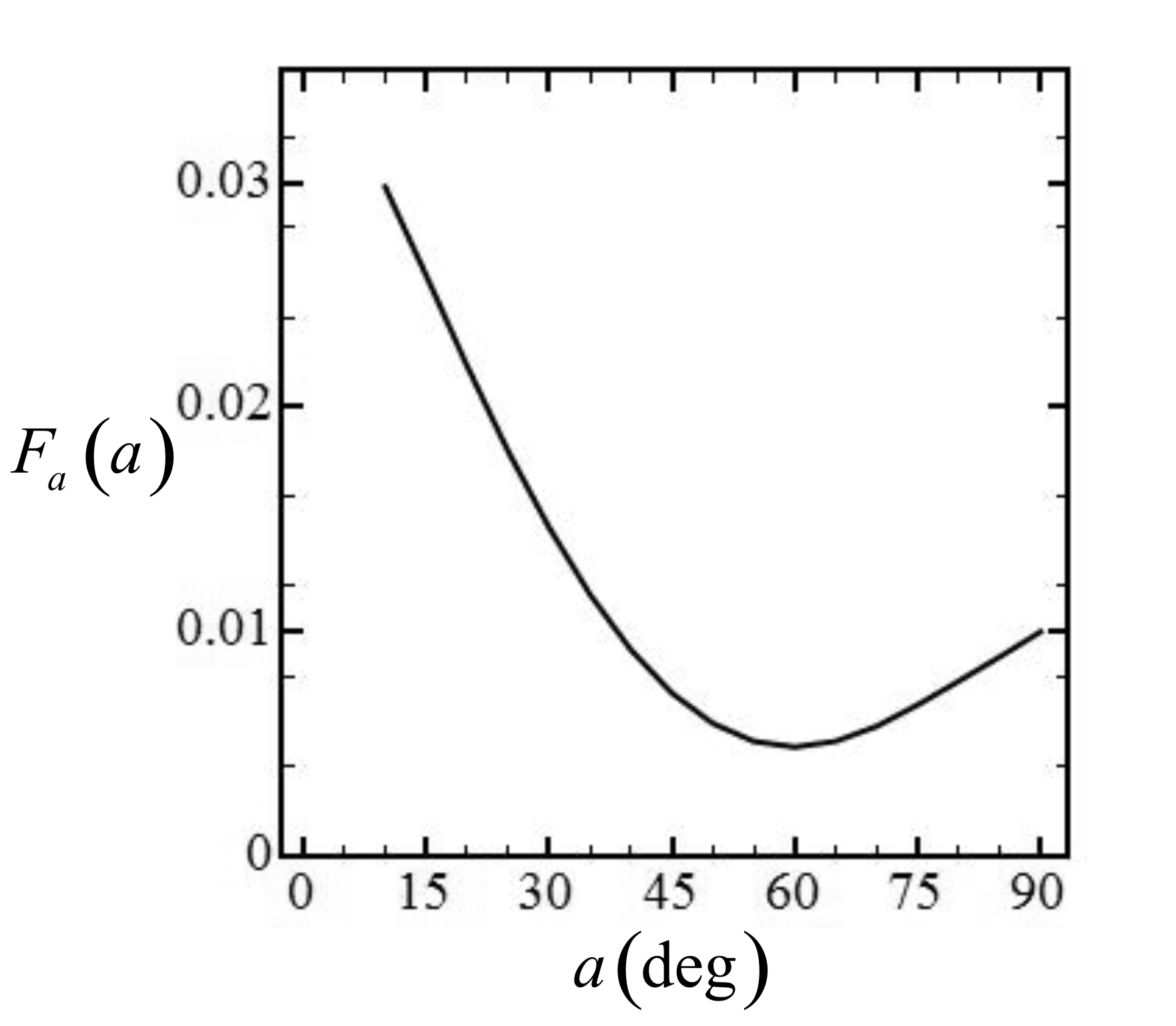
On the other hand, the same analysis for the FIDO models produces fruitful results. Figure 22 is similar to Fig. 21 but for the FIDO models. The left-hand column shows that there are $w_{\alpha_{i}}$ sets that fit the observed statistics almost perfectly along $\delta$ and $\Delta$ axes and the right-hand column panels imply that these optimizing $w_{\alpha_{i}}$ sets are close enough to each other so that their average values still result in model distributions that are in perfect agreement with the Fermi observations. The success of FIDO models allows the use of the weights $w_{\alpha_{i}}$ as estimators of the intrinsic distribution function of $\alpha$ in observed pulsars. Figure 23 shows the probability distribution function $F_{\alpha}(\alpha)$ estimated from the optimizing weights $w_{\alpha_{i}}$ used in the right-hand column of Fig. 22. We observe that there is a significant probability excess for low inclination angles $(\alpha<45^{\circ})$. For higher inclination angles the probability decreases even though it seems that there is an increasing trend for very high $\alpha$. The form of the $\alpha$ distribution function is consistent either to an initial $\alpha$ function predominant in low $\alpha$ values or to an initial $\alpha$ function that has been modified considerably by the alignment torques applied on the stellar surface. Finally, we note that this distribution function represents the distribution of the existing pulsars and should not be confused with the $\alpha$ distribution of the observed pulsars. The latter distribution depends also on the probability of observation with respect to $\alpha$.

Figure 22.— Same as Fig. 21 but for the FIDO models. In (a), (c) we see an almost perfect match (between the models and the observations) for the corresponding optimum $\alpha$ distributions. In (b), (d) the mean $\alpha$ distribution of those adopted in (a), (c) still produce histograms in good agreement with the observations.

Figure 23.— The optimum mean $\alpha$ probability distribution function $F_{a}(a)$ adopted in Fig. 22b, d.

6. Conclusions

In this paper we studied the radiation patterns of $\gamma$-radiation in dissipative pulsar magnetospheres, assuming the emission is due to curvature radiation. This study enabled us to identify models that successfully reproduce the observed $\gamma$-ray light-curve phenomenology.

We considered series of dissipative pulsar magnetosphere models corresponding to all macrophysical current density prescriptions used in the literature. These models cover, in general, the entire spectrum of solutions from the near-vacuum to the near Force-Free regime and provide the intrinsic distributions of parallel electric field components. These depend on the adopted conductivity value involved in each dissipative macrophysical prescription. In general, as the conductivity evolves from low to intermediate values, both the field geometry and the values of the parallel electric field components change considerably. However, for sufficiently large conductivity values ($\sigma\buildrel>\over{\sim}10\Omega$) the geometry stabilizes to near Force-Free structure, but the accelerating parallel electric components remain sensitive to the conductivity with their values decreasing with increasing $\sigma$. For each model, we considered charged particles $(e^{+},e^{-})$ uniformly distributed on the polar caps and we integrated their trajectories from the neutron star surface up to a distance 2.5 times that of the light-cylinder radius. We assumed that the particle velocities consist of two components: (a) a drift component perpendicular to the plane defined by the electric and magnetic fields and (b) a component parallel to the magnetic field, determined by the requirement that the total velocity be $v=c$. The trajectory integration includes the acceleration of the particles by the electric fields of the specific model magnetosphere and their energy losses due to curvature radiation with the local radius of curvature provided by the model field structure. From this calculation we produce sky-maps and the corresponding $\gamma$-ray light-curves based on the physical properties of the models. Our ultimate goal was to compare the $\gamma$-ray light-curve phenomenology predicted by the models with those of the observed pulsars in the Second Fermi Pulsar Catalog (2PC).

Initially, we considered models of uniform conductivity in the open field line regions (in the closed field line region the Force-Free condition has been applied i.e. infinite conductivity). For low conductivity values the radiation is produced mainly in the inner magnetosphere, well within the light-cylinder. An increase of conductivity pushes the radiation emission to higher altitude while the solution gradually starts forming features of the Force-Free solutions (e.g. current sheets). The formation of an equatorial current sheet outside the light-cylinder that extends inside the light-cylinder along a part of the separatrix induces high parallel electric components in the nearby regions. For high conductivity values ($10\Omega<\sigma<30\Omega$) a significant part of the total radiation is produced in regions near the equatorial current sheet outside the light-cylinder and for very high values ($\sigma\gg 30\Omega$) all radiation originates in this region. However, the emission is not uniform in this region near the equatorial current sheet since it is modulated by the inclination-dependent distribution of the accelerating parallel electric field components within the light-cylinder. The emission in these equatorial CS regions is more efficient the higher the Lorentz values $\gamma_{L}$ of the radiating particles. We found that the highest values of $\gamma_{L}$ are those of the particles that encounter the highest parallel electric fields within the LC. These highest field regions are the segments of the separatrix along which the return current flows, in current sheet form, down to the stellar surface. This region is uniform over the separatrix only for the aligned rotator but as the inclination angle increases the current sheet region of the separatrix decreases and vanishes for the limiting case of the orthogonal rotator (see Fig. 1). This effect makes the emission in the region near the equatorial current sheet non-uniform especially for the high inclination angles.

The fitting of model light curves to the observed light curves picks out the best parts of parameter space for each model, but does not statistically test the ability of the model phase space to match the entire distribution of light curve properties. Instead, we statistically compared the distribution of the radio-lag ($\delta$) vs peak-separation ($\Delta$) of the model and observed light curves, assuming (for the model light-curves) that the radio emission is produced near the magnetic poles, not far above the stellar surface (compared to the LC radius).

This comparison revealed that the low conductivity models give the poorest match to the observed $\delta$ vs $\Delta$ distribution, giving the largest radio-lags of all the models. The higher conductivity models perform better, as the emission moves outward and the regions near the equatorial current sheet become gradually active. However, even for very high conductivity values there are still model points on the $(\delta-\Delta)$ diagram that do not lie near the observed ones. We note also that for these high conductivities the $\gamma_{L}$ values of the particles in the emitting regions do not exceed $\simeq 10^{6}$ and the corresponding photon energies are well below GeV. Nevertheless, this analysis clearly showed that the high conductivity models did best at matching the data. Moreover, this study identified the different emission regions near the equatorial current sheet.

The equatorial current sheet had already been proposed as a candidate source region of the $\gamma$-ray emission (Contopoulos & Kalapotharakos, 2010; Bai & Spitkovsky, 2010; Pétri, 2011; Arka & Dubus, 2013). These studies assumed uniform (azimuthally symmetric) emissivity or constant $\gamma_{L}$ values over the emitting region. Although we demonstrated the systematically higher radio-lags of the light-curves of these models, they seem to produce the observed trend in the $\delta-\Delta$ diagram, and are statistically better than the high conductivity dissipative models discussed above.

The relatively good performance of the models that assume ad hoc uniform emission near the equatorial current sheet and of the high, uniform conductivity dissipative models, that produce emission in regions near the equatorial current sheet that is modulated by the accelerating electric field components in the inner magnetosphere (within the light-cylinder), motivated us to search for models that produce most of the $\gamma$-ray emission from regions near the equatorial current sheet, but this time modulated by the local physical properties. We found a simple macrophysical model that statistically best reproduces the $\gamma$-ray light-curve phenomenology.

Such a model assumes that the magnetosphere is in an exact Force-Free regime inside the light-cylinder and dissipative outside (FIDO) the light-cylinder. This implies that the conductivity in the inner magnetosphere is infinite while in the outer magnetosphere it is finite, though still high. The $\gamma$-ray emission is still produced in a region near the equatorial current sheet but the emission distribution is different from that of the uniform conductivity models discussed above. The success of this kind of model consists mainly in that: (a) The $\gamma$-ray emission is not present for low observer angle values $(\zeta)$ and high inclination angles $(\alpha)$ due to the smaller accelerating electric field in the corresponding regions. The emission at these angles would come from a region that is relatively close to the rotational equator, eliminating some points of the $(\delta-\Delta)$ diagram of higher radio-lag values $(\delta)$. (b) The $\gamma$-ray emission is asymmetric across the equatorial current sheet, being more effective on the side that comes from the leading part of the polar cap; this side produces lower radio-lag values $(\delta)$.

We note also that the light curves we get in FIDO models for $\sigma=30\Omega$ changes only slightly for much higher conductivity values ($\lesssim 1000\Omega$). However, the magnitude of the finite conductivity value $(\sim 30\Omega)$ of FIDO models, presented in Section 5, seems to be important. Much lower conductivity values $(\ll 30\Omega)$ are expected to destroy the equatorial current sheet and the associated high accelerating electric field components. Moreover, the value of conductivity of FIDO models produces accelerating electric field components and associated voltages that are able to produce Lorentz factors $(\gamma_{L})$ up to the order of $10^{7.5}$. With these $\gamma_{L}$ values the associated photon energies can reach up to GeVs. Much higher conductivity values $(\gg 30\Omega)$ result in a photon energy that barely exceeds MeVs even though they keep a similar emission pattern (with narrower pulses). Thus, the FIDO value seems to support both the observed light-curve phenomenology and the observed photon cut-off energies. We constructed the FIDO model of $\gamma$-ray emission with the goal of reproducing the observed $\gamma$-ray light-curve phenomenology, and its success in statistically best matching the observations is important in itself. Now, the fact that the model emitting regions that emerge naturally as a result of physical properties of the solutions also accelerate particles to $\gamma$-ray emitting energies makes them even more significant.

The FIDO emission geometry and sky-maps, while distinctly different from any of the previously proposed $\gamma$-ray emission models, do have elements of each. Slot-gap (SG) models (Muslimov & Harding, 2004) have a two-pole caustic (Dyks & Rudak, 2003) emission geometry, produced by uniform emission along the closed/open field boundary of both magnetic poles from the neutron star surface to the light-cylinder. An observer thus sees emission from both magnetic poles and there is emission throughout the sky-map and at all pulse phases. Outer-gap (OG) models (Romani & Yadigaroglu, 1995) have a one-pole caustic geometry, produced by emission along the closed/open field boundary but only in the outer magnetosphere above the null charge surface. An observer thus sees emission from only one magnetic pole and much of the sky-map is devoid of emission for smaller inclination angles, with no emission at off-peak pulse phases. The FIDO model has intrinsically a two-pole geometry, like the SG model, but no emission at low altitudes or at off-peak phases, like the OG model. Although the location of emission in the FIDO model is similar to that of the current sheet models, the emission pattern (for high $\alpha$ values) looks quite different, with emission over much less of the sky-map.

The FIDO models imply that the parallel electric field is efficiently screened in the inner magnetosphere, thus prohibiting any modulation from the inner magnetosphere of the emission in regions near the equatorial current sheet. This implies in turn that pair cascades must be operating along all open field lines; something that seems to be supported by recent studies of time-dependent pair cascades (Timokhin, 2010; Timokhin & Arons, 2013; Chen & Beloborodov, 2013). An explanation of why these cascades are not efficient enough to screen the accelerating electric fields in the outer magnetosphere could be the following: on the one hand, the large number density of the charges produced above the polar caps decreases with distance from the stellar surface due to the diverging flow lines. On the other hand, the corresponding Goldreich-Julian density could either decrease slower than the number density or increase with the distance from the stellar surface (especially for the flows that pass through regions near the equatorial current sheet; see eq. 6 and eq. 53 in Contopoulos et al. 1999 and Timokhin 2006, respectively). This effect generally increases the number of particles required for efficient screening of the accelerating electric fields. This increased demand on screening arises rather abruptly near the light-cylinder, where the required Goldreich-Julian density is high (in regions near the equatorial current sheet). Even though the demand for charges increases, the ability of new particle creation is small due to the significantly smaller magnetic fields and the low probability of photon-photon interactions.

We note that the theoretical consideration discussed above remain speculative as long as its validity is not verified by self-consistent studies of the microphysical processes. Certainly this will act as a driver for these kind of studies. The $\gamma$-ray luminosities produced by the FIDO models should also be investigated. The microphysical description presented in this paper allows the derivation of spectra (averaged and phase-resolved) that can be compared directly with the Fermi observations. We plan to present the study of the energetics of FIDO models in a forthcoming paper. We expect this study to put stronger constraints on the models and to help in the deeper understanding of the underlying microphysics.

References

- Abdo et al. (2009) Abdo, A. A., et al. 2009, ApJ, 696, 1084
- Abdo et al. (2013) —. 2013, ApJSS, 208, 17
- Arka & Dubus (2013) Arka, I., & Dubus, G. 2013, A&A, 550, A101
- Bai & Spitkovsky (2010) Bai, X.-N., & Spitkovsky, A. 2010, ApJ, 715, 1282
- Berenger (1994) Berenger, J. P. 1994, Journal of Computational Physics, 114, 185
- Berenger (1996) —. 1996, Journal of Computational Physics, 127, 363
- Bogovalov (1999) Bogovalov, S. V. 1999, A&A, 349, 1017
- Chen & Beloborodov (2013) Chen, A. Y., & Beloborodov, A. M. 2013, ApJ, 762, 76
- Cheng et al. (1986) Cheng, K. S., Ho, C., & Ruderman, M. 1986, ApJ, 300, 500
- Contopoulos & Kalapotharakos (2010) Contopoulos, I., & Kalapotharakos, C. 2010, MNRAS, 404, 767
- Contopoulos et al. (1999) Contopoulos, I., Kazanas, D., & Fendt, C. 1999, ApJ, 511, 351
- Deutsch (1955) Deutsch, A. J. 1955, Annales d’Astrophysique, 18, 1
- Dyks & Harding (2004) Dyks, J., & Harding, A. K. 2004, ApJ, 614, 869
- Dyks & Rudak (2003) Dyks, J., & Rudak, B. 2003, ApJ, 598, 1201
- Goldreich & Julian (1969) Goldreich, P., & Julian, W. H. 1969, ApJ, 157, 869
- Gruzinov (1999) Gruzinov, A. 1999, ArXiv Astrophysics e-prints
- Gruzinov (2005) —. 2005, Physical Review Letters, 94, 021101
- Gruzinov (2008) —. 2008, ArXiv e-prints
- Harding et al. (2011) Harding, A. K., DeCesar, M. E., Miller, M. C., Kalapotharakos, C., & Contopoulos, I. 2011, ArXiv e-prints
- Hewish et al. (1968) Hewish, A., Bell, S. J., Pilkington, J. D. H., Scott, P. F., & Collins, R. A. 1968, Nature, 217, 709
- Kalapotharakos & Contopoulos (2009) Kalapotharakos, C., & Contopoulos, I. 2009, A&A, 496, 495
- Kalapotharakos et al. (2012a) Kalapotharakos, C., Contopoulos, I., & Kazanas, D. 2012a, MNRAS, 420, 2793
- Kalapotharakos et al. (2012b) Kalapotharakos, C., Harding, A. K., Kazanas, D., & Contopoulos, I. 2012b, ApJL, 754, L1
- Kalapotharakos et al. (2012c) Kalapotharakos, C., Kazanas, D., Harding, A., & Contopoulos, I. 2012c, ApJ, 749, 2
- Komissarov (2006) Komissarov, S. S. 2006, MNRAS, 367, 19
- Li et al. (2012a) Li, J., Spitkovsky, A., & Tchekhovskoy, A. 2012a, ApJL, 746, L24
- Li et al. (2012b) —. 2012b, ApJ, 746, 60
- McKinney (2006) McKinney, J. C. 2006, MNRAS, 368, L30
- Meier (2004) Meier, D. L. 2004, ApJ, 605, 340
- Muslimov & Harding (2004) Muslimov, A. G., & Harding, A. K. 2004, ApJ, 606, 1143
- Palenzuela (2013) Palenzuela, C. 2013, MNRAS, 431, 1853
- Parfrey et al. (2012) Parfrey, K., Beloborodov, A. M., & Hui, L. 2012, MNRAS, 423, 1416
- Pétri (2011) Pétri, J. 2011, MNRAS, 412, 1870
- Pétri (2012) —. 2012, MNRAS, 424, 605
- Rankin (1983) Rankin, J. M. 1983, ApJ, 274, 333
- Romani & Yadigaroglu (1995) Romani, R. W., & Yadigaroglu, I.-A. 1995, ApJ, 438, 314
- Scharlemann & Wagoner (1973) Scharlemann, E. T., & Wagoner, R. V. 1973, ApJ, 182, 951
- Spitkovsky (2006) Spitkovsky, A. 2006, ApJL, 648, L51
- Tchekhovskoy et al. (2013) Tchekhovskoy, A., Spitkovsky, A., & Li, J. G. 2013, MNRAS, 435, L1
- Timokhin (2006) Timokhin, A. N. 2006, MNRAS, 368, 1055
- Timokhin (2010) —. 2010, MNRAS, 408, 2092
- Timokhin & Arons (2013) Timokhin, A. N., & Arons, J. 2013, MNRAS, 429, 20
- Uzdensky (2003) Uzdensky, D. A. 2003, ApJ, 598, 446
- Wolfram Research, Inc. (2010) Wolfram Research, Inc. 2010, Mathematica Version 8.0 (Champaign, Illinois: Wolfram Research, Inc.)
- Yu (2011) Yu, C. 2011, MNRAS, 411, 2461