Search for global $f$-modes and $p$-modes in the ⁸B neutrino flux

Abstract

The impact of global acoustic modes on the ⁸B neutrino flux time series is computed for the first time. It is shown that the time fluctuations of the ⁸B neutrino flux depend on the amplitude of acoustic eigenfunctions in the region where the ⁸B neutrino flux is produced: modes with low $n$ (or order) that have eigenfunctions with a relatively large amplitude in the Sun’s core, strongly affect the neutrino flux; conversely, modes with high $n$ that have eigenfunctions with a minimal amplitude in the Sun’s core have a very small impact on the neutrino flux. It was found that the global modes with a larger impact on the ⁸B neutrino flux have a frequency of oscillation in the interval $250\;\mu{\rm Hz}$ to $500\;\mu{\rm Hz}$ (or a period in the interval $30$ minutes to $70$ minutes), such as the $f$-modes ($n=0$) for the low degrees, radial modes of order $n\leq 3$, and the dipole mode of order $n=1$. Their corresponding neutrino eigenfunctions are very sensitive to the solar inner core and are unaffected by the variability of the external layers of the solar surface. If time variability of neutrinos is observed for these modes, it will lead to new ways of improving the sound speed profile inversion in the central region of the Sun.

1. Introduction

Over the last three decades, the neutrino physics community has been able to characterize some of the basic properties of neutrinos, namely, their oscillatory nature between flavors in a vacuum as well as in matter (Pontecorvo, 1958; Wolfenstein, 1978; Mikheyev & Smirnov, 1986), and fine-tune the properties of the nuclear reactions where neutrinos are produced in the Sun’s core. Although some important questions remain unsolved, the basic theory of neutrino physics is by now well understood (e.g., Bilenky, 2010).

The high quality of neutrino data available from current and future experiments (e.g, Abe et al., 2011; Bellini et al., 2010) will provide a way to make accurate diagnostics of the solar nuclear region, allowing us to test the shortcomings and limitations of the present standard solar model (SSM; Turck-Chieze & Lopes, 1993; Turck-Chieze et al., 2010; Lopes & Turck-Chieze, 2013).

Our understanding of the physical processes occurring in the Sun’s interior has progressed significantly due to the use of two complementary solar probes: solar neutrino fluxes and helioseismology data. In particular, it was possible to infer some of the basic dynamic properties of plasma in the Sun’s core, like the ones caused by the presence of magnetic fields, rotation and other flow motions (e.g., Turck-Chieze & Couvidat, 2011). Furthermore, this combined analysis of data was also used to test fundamental concepts in physics (e.g., Lopes & Silk, 2003; Casanellas et al., 2012) or to study the properties of dark matter (e.g., Lopes & Silk, 2002, 2010a, 2010b, 2012). In the latter case, the Sun is used as a cosmological tool, following a research strategy quite common in modern cosmology of using stars to constrain the properties of dark matter (e.g., Kouvaris & Tinyakov, 2011; Casanellas & Lopes, 2013).

Helioseismology, by means of sophisticated inversion techniques, has been able to infer some fundamental quantities related to the thermodynamics and dynamics properties of the Sun’s interior (Turck-Chieze & Couvidat, 2011). The two leading results worth mentioning are speed of sound (Basu et al., 2009; Turck-Chieze et al., 2001, 2004) and the differential rotation (Thompson et al., 1996) profiles. These results are obtained between the layers $0.8R_{\odot}$ (beneath the photosphere) and $0.1R_{\odot}$ (nuclear region). This achievement was possible due to high precision frequency measurements of several thousands of vibration acoustic modes with a precision better than $10^{-5}$ (see Turck-Chieze & Couvidat, 2011, and references therein). Unfortunately, the physics in the solar inner core is still largely unknown due to the fact that only a small number of acoustic modes are sensitive to that region and among these only a few have been successfully detected (Bertello et al., 2000; Garcia et al., 2001; Jimenez & Garcia, 2009). Naturally, the diagnostic of the solar core could improve significantly if the discovery of gravity modes is confirmed (Turck-Chieze et al., 2004; Garcia et al., 2007; Turck-Chieze et al., 2012).

Solar neutrino flux time fluctuations have been studied for several decades, mainly focusing on finding evidence of the solar magnetic cycle and day–night earth effects (e.g., Lisi et al., 2004; Sturrock et al., 2005; Fogli et al., 2005; Chauhan, 2006).

This work focuses on the impact of global acoustic mode oscillations on solar neutrino fluxes. Some of these acoustic modes propagate to the deepest layers of the Sun’s nuclear region, and perturb the local temperature. Global acoustic modes with small order are very sensitive to the central core and are not perturbed by the surface. The space instrument Global Oscillations at Low Frequencies (GOLF) has begun to detect some of these modes although not all of them have yet been identified due their small amplitudes at the surface. See Table 1 and the review (Turck-Chieze & Lopes, 2012) which gives a synthesis of the performances of these modes.

In principle, time variations of neutrino flux measurements could provide a way to measure the frequencies of such modes with a very small amplitude at the surface, without the variability related to the complex structure of the solar upper layers, caused by non-adiabaticity, turbulent convection, sub-photospheric differential rotation, magnetic activity and solar oblateness (Howe, 2009).

In this Letter, we discuss the possibility of detecting global acoustic oscillations of low order in solar neutrino flux fluctuations. It is true that global modes of very high order have a small amplitude in the Sun’s core, but global modes of low order have quite a large amplitude in the core as well as on the surface. There is the distinct possibility of observing them in the solar neutrino flux fluctuations, or in the case that the observations are not confirmed, it will be possible to put an upper bound on their amplitude in the Sun’s core. We estimate for the first time the impact of global acoustic modes in the ⁸B neutrino flux and predict the global modes which are more likely to be found in solar neutrino flux time series.

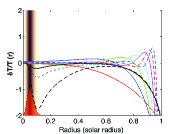
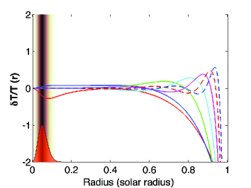
Figure 1.— The region of emission of ⁸B neutrinos (brown dashed area) and their flux $\Phi$ (r) (orange area). The $(\delta T/T)_{ln}$ eigenfunctions are drawn for selected radial ($l=0$) and quadrupole ($l=2$) acoustic modes computed for the current solar model: (a) $p_{1},\cdots,p_{7}$ radial ($l=0$) modes + $f$ modes for $l=3,4,5$; (b) $f$ and $p_{1},\cdots,p_{6}$ quadrupole ($l=2$) modes. The color for modes $l=0$ and $l=2$ runs from the lower to the higher value of $n$ in the following sequence: red, blue, green, cyan, magenta, dashed red and dashed blue The $f$ modes of degree $l=3$, $l=4$ and $l=5$ correspond to continuous, dotted and dashed back curves, respectively. For convenience, $(\delta T/T)_{ln}$ of the $l=0$ and $l=2$ modes were normalized to the value 4, the $f$ modes of $l=3$, $l=4$ and $l=5$ to the value 8 and $\Phi(r)$ to the value 1.

Table 1⁸B Neutrino Flux Variations
Caused by Acoustic Modes

Mode	Frequency [obs]	Frequency [th]	${\cal B}_{ln}$
$(l,n)$	($\mu Hz$)	($\mu Hz$)
$(l=\cdots,\;n=0)$			$\times 10^{0}$
$2$ $f$	$-$	$347.10$	$0.8069$
$3$ $f$	$-$	$386.65$	$0.9704$
$4$ $f$	$-$	$405.43$	$2.0608$
$5$ $f$	$-$	$415.08$	$5.7283$
$(l=0,n=\cdots)$			$\times 10^{-1}$
$p_{1}$	$258.60\pm 0.030$	$258.43$	$1.5280$
$p_{2}$	$-$	$404.36$	$1.9924$
$p_{3}$	$535.75\pm 0.010$	$535.57$	$1.4123$
$p_{4}$	$-$	$679.87$	$0.9378$
$p_{5}$	$825.23\pm 0.030$	$824.51$	$0.6264$
$p_{6}$	$972.612\pm 0.005$	$971.76$	$0.4376$
$p_{7}$	$-$	$1116.94$	$0.3221$
$p_{8}$	$1263.215\pm 0.01$	$1262.31$	$0.2336$
$p_{9}$	$1407.49\pm 0.01$	$1406.39$	$0.1721$
$p_{10}$	$1548.304\pm 0.01$	$1547.44$	$0.1238$
$(l=1,n=\cdots)$			$\times 10^{-2}$
$p_{1}$	$-$	$283.80$	$21.674$
$p_{2}$	$-$	$448.38$	$2.5458$
$p_{3}$	$-$	$596.67$	$1.6681$
$p_{4}$	$-$	$746.41$	$1.2171$
$p_{5}$	$-$	$893.19$	$0.9868$
$p_{6}$	$1039.465\pm 0.003$	$1038.95$	$0.7835$
$p_{7}$	$1185.60\pm 0.05$	$1184.84$	$0.6448$
$p_{8}$	$1329.63\pm 0.01$	$1328.87$	$0.5188$
$p_{9}$	$1472.86\pm 0.02$	$1472.20$	$0.4065$
$p_{10}$	$1612.746\pm 0.01$	$1611.99$	$0.3210$
$(l=2,n=\cdots)$			$\times 10^{-3}$
$p_{1}$	$-$	$382.26$	$177.67$
$p_{2}$	$-$	$514.48$	$5.2266$
$p_{3}$	$-$	$664.06$	$0.6738$
$p_{4}$	$-$	$811.33$	$0.2446$
$p_{5}$	$-$	$959.23$	$0.5623$
$p_{6}$	$-$	$1104.28$	$0.6874$
$p_{7}$	$-$	$1249.78$	$0.7097$
$p_{8}$	$1394.68\pm 0.01$	$1393.68$	$0.6865$
$p_{9}$	$1535.865\pm 0.006$	$1535.08$	$0.6138$
$p_{10}$	$1674.534\pm 0.013$	$1673.80$	$0.5455$
$(l=3,n=\cdots)$			$\times 10^{-4}$
$p_{1}$	$-$	$415.95$	$517.5$
$p_{2}$	$-$	$564.69$	$15.608$
$p_{3}$	$-$	$718.30$	$4.2462$
$p_{4}$	$-$	$866.47$	$1.6805$
$p_{5}$	$-$	$1014.41$	$0.5456$
$p_{6}$	$-$	$1160.82$	$0.0577$
$p_{7}$	$-$	$1305.85$	$0.4158$
$p_{8}$	$-$	$1450.10$	$0.6137$
$p_{9}$	$-$	$1590.63$	$0.7015$
$p_{10}$	$1729.74\pm 0.02$	$1728.34$	$0.7355$

2. Propagation of acoustic waves towards the core of the Sun

As we are looking for the propagation of acoustic waves generated in the upper layers of the convection zone by turbulence (e.g., Goldreich et al., 1994), any acoustic oscillation is regarded as a perturbation of the internal structure of the star. Therefore, any perturbed thermodynamic quantity $f$ is such that $f=f_{o}+\delta f$, where $f_{o}$ and $\delta f$ denote the equilibrium value and the Lagrangian perturbation of $f$.  It follows that for each eigenmode of vibration of degree $l$ and order $n$ (where the contribution of the magnetic field and rotation is considered negligible) that there is an unique eigenfrequency $\omega_{ln}$ and an unique set of eigenfunctions (e.g., Unno et al., 1989). For example, the perturbation of temperature will have an unique radial eigenfunction $\delta T_{ln}(r)$. Table 1 shows the frequencies of the radial and non-radial acoustic modes computed for the current SSM (Turck-Chieze & Lopes, 1993; Morel, 1997; Turck-Chieze et al., 2010; Lopes & Turck-Chieze, 2013). This solar model is identical to others published in the literature (e.g., Serenelli et al., 2011). As shown in Table 1, the difference between theoretical $[th]$ and observational $[obs]$ frequencies is smaller than $0.1\%$ (Bertello et al., 2000; Garcia et al., 2001; Turck-Chieze et al., 2004; Jimenez & Garcia, 2009).

Figure 1 shows $\delta T_{ln}(r)$ for $p_{n}$ modes with $l=0$ and $l=2$ and the $f$ modes for $l=2,\cdots,5$. Global acoustic modes based on the eigenfunction behavior can be classed into two types: modes of high $n$ – for which the amplitude of the radial eigenfunction is very small near the center of the star and its maximum occurs near the surface; and modes of lower $n$ – for which the amplitude of the radial eigenfunction is quite large near the center of the star. Examples of the latter type are $p_{1}$ and $p_{2}$ radial, dipole and quadrupole modes, as well as the $f$ quadrupole and octapole modes. Somehow the eigenfunctions of such modes of low $n$ in the Sun’s core exhibit a behavior identical to that of the eigenfunctions of gravity modes (Provost et al., 2000).

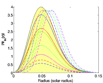
Figure 2.— The modulus of neutrino survival eigenfunctions $|\Psi_{ln}|$, for a selected number of acoustic modes (see Table 1): (a) $p_{1},\cdots,p_{7}$ radial ($l=0$) modes corresponding to the same temperature eigenfunctions shown in Figure 1(a) (the same color scheme). (b) $p_{1}$ dipole ($l=1$) mode ($-.-$ red line), $f$ quadrupole ($l=2$) mode ($-.-$ blue line), $f$ octupole ($l=3$) mode ($-.-$ green line) $f$ mode for $l=4$ ($--$ cyan line) $f$ mode for $l=5$ ($--$ magenta line). $|\Psi_{ln}|$ is a dimensionless quantity computed using Equation (5). The source of ⁸B neutrino flux, $\Phi(r)$, is shown as a light-yellow area. The functions $\Phi(r)$ are normalized to $4$ to facilitate the comparison with other curves. Similarly, the functions $|\Psi_{ln}|$ in the case (b) are normalized to 3.8.

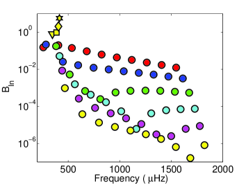
Figure 3.— ${\cal B}_{ln}$ for global modes: (a) $p_{n}$ ($n=1,\cdots,10$) for $l=0$ (red bullet), $l=1$ (blue bullet), $l=2$ (green bullet), $l=3$ (cyan bullet), $l=4$ (magenta bullet) and $l=5$ (yellow bullet). (b) $f$-mode for $l=2$ (yellow triangle), $l=3$ (yellow square), $l=4$ (yellow diamond) and $l=5$ (yellow hexagram). $B_{ln}$ is computed as proposed by Equation (4). See Table 1 for numerical values of ${\cal B}_{ln}$.

The propagation of acoustic waves toward the Sun’s center perturbs the local thermodynamic structure, such as the chemical abundances, the density $\rho$ and the temperature $T$, triggering fluctuations in the energy generation rate $\epsilon$ of the different nuclear reactions, in particular the ones related to the production of solar neutrinos. Therefore, the neutrino flux $\Phi(r)$ reads (e.g., Kippenhahn & Weigert, 1994):

$$\frac{\delta\Phi}{\Phi}=\frac{\delta\rho}{\rho}+\vartheta\frac{\delta T}{T}\simeq\zeta_{o}\frac{\delta T}{T},$$ (1)

where $\vartheta$ and $\zeta_{o}$ are constants. In the derivation of this result, $\delta\Phi$ is considered proportional to $\delta\epsilon$, such that $\delta\Phi/\Phi\approx\delta\epsilon/\epsilon$. The second (approximated) equality of Equation (1) is obtained as follows: for adiabatic non-radial acoustic oscillations (which are valid in the interior of the Sun) the following relation is valid ${\delta\rho}/{\rho}=\left(\Gamma_{3}-1\right)^{-1}{\delta T}/{T}$, where $\Gamma_{3}-1=\left(\partial T/\partial\rho\right)_{s}$ is the derivative being taken at constant specific entropy $s$ (e.g., Unno et al., 1989). In the Sun’s core, as the plasma is fully ionized, $\Gamma_{3}=5/3$. It is also assumed that the average cross-section between reagent particles is proportional to the $T^{\vartheta}$ where $\vartheta$ is an exponent, and the perturbation of the mass fractions of the reacting particles are considered negligible. In particular, the production of the ⁸B neutrino flux, $\Phi$, is estimated to be proportional to $T_{c}^{24}$ where $T_{c}$ is the temperature at the center of the Sun (Bahcall & Ulmer, 1996). Accordingly, if the value of $\vartheta$ is taken to be equal to $24$ then $\zeta_{o}\equiv 3/2+\vartheta=25.5$. This result shows that the relative variation on the neutrino flux is $25.5$ times larger than the temperature perturbation that has caused it.

It follows that the total neutrino flux when perturbed by an acoustic mode of frequency $\omega_{ln}$ is given by

$$\phi_{ln}(t)=\phi_{o}+\Delta\phi_{ln}(t),$$ (2)

where $\phi_{o}$ is the total neutrino flux (independent of time) as computed by the SSM (equilibrium model) and $\Delta\phi_{ln}(t)$ is the amount of neutrino flux produced or suppressed by the acoustic mode of vibration. By integrating the Equation (1) for the total mass of the star, $\Delta\phi_{ln}(t)$ reads

$$\Delta\phi_{ln}(t)={\cal A}_{ln}\;\zeta_{o}\;{\cal B}_{ln}\;\phi_{o}\;\;e^{-i\omega_{ln}t}\;e^{-\eta_{ln}t},$$ (3)

where ${\cal A}_{ln}$ is an amplitude related to the excitation source of global modes and ${\cal B}_{ln}$ is a quantity that determines the fraction of the total neutrino flux which is affected by the mode. ${\cal B}_{ln}$ reads

$${\cal B}_{ln}=\int_{0}^{R}\Psi_{ln}(r)dr,$$ (4)

where $\Psi_{ln}$ in the neutrino survival eigenfunction. $\Psi_{ln}$ reads

$$\Psi_{ln}=C_{\phi}^{-1}\;\left(\frac{\delta T}{T}\right)_{ln}\Phi\;\rho\;4\pi r^{2},$$ (5)

where $C_{\phi}$ is a normalization constant given by $C_{\phi}=\int\Phi(r)4\pi\rho(r)r^{2}\;dr$. Figure 2 presents the function $|\Psi_{ln}|$ for several modes, and Figure 3 and Table 1 show the values of ${\cal B}_{ln}$. $\Psi_{ln}$ results from the superposition of the eigenfunction $\delta T_{ln}$ with $\Phi(r)$, as schematically illustrated in Figure 1. The $|\Psi_{ln}|$ functions have an identical shape for all the modes, the difference being only in the magnitude of $|\Psi_{ln}|$, which depends on the magnitude of $\delta T_{ln}$ within the region where the ⁸B neutrino flux is produced (see Figure 2). The contribution of $\delta T_{ln}$ is more important in the case of low $n$ global modes, for which the amplitude of $\delta T_{ln}$ is large in the Sun’s core, which leads to a large value of ${\cal B}_{ln}$. Furthermore, in general, radial acoustic modes have a more important impact on the ⁸B neutrino flux than other global modes, and consequently produce a relatively larger value of ${\cal B}_{ln}$, as shown in Figure 3 and Table 1.

Clearly, the impact on the neutrino fluxes is larger for the $f$-modes and the $p_{n}$ modes of low degree. The strong impact on the $f$-modes of low degree is related to the fact that their temperature eigenfunctions have their maximum near the center of the Sun (see Figure 1), which also corresponds to the maximum of the kinetic energy of the mode, as shown by Provost et al. (2000). These $f$-modes are quite distinct from $f$-modes of high degree which have their maximum amplitude located near the surface (Schou et al., 1997). In fact, in the solar core these low degree $f$-modes have an amplitude with the same order as the low order gravity modes.

Among the $p_{n}$ modes, we notice the fact that the radial modes with $n$ equal to $1$, $2$ and $3$ have a larger impact on the ⁸B neutrino flux than other $p_{n}$ modes. This is due to the fact that the temperature eigenfunction of these modes has a relatively large value within the region of production of the ⁸B neutrinos (see Figure 1).

Presently, the excitation of acoustic and gravity waves is attributed to the random motions of convective elements in the upper layers, due to the Reynolds stress tensor or the advection of turbulent fluctuations of entropy (e.g., Goldreich et al., 1994; Samadi et al., 2008). The prediction of their amplitudes in the solar core is highly unreliable due to the uncertainty associated with the excitation and dumping mechanisms. Nevertheless, we make a qualitative estimation of their amplitudes using observational information from acoustic modes.

The amplitude for neutrino flux fluctuations $|\Delta\phi_{ln}/\phi_{o}|_{\rm max}$ can be computed from the amplitude of the temperature eigenfunction ${\cal A}_{ln}$. From Equation (3), one obtains $|\Delta\phi_{ln}/\phi_{o}|_{\rm max}=25.5\;{\cal A}_{ln}{\cal B}_{ln}$ (with $\zeta_{o}=25.5$). Following a procedure used to compute the surface amplitude of oscillations, ${\cal A}_{nl}$ is estimated from ${\cal A}_{nl}\approx 2/3\;\delta\rho/\rho$ (for $\Gamma_{3}\sim 5/3$) and $\delta\rho/\rho=v_{\rm ex}/c_{\rm s}$, where $v_{\rm ex}$ is the fluid velocity related with the excitation of acoustic modes and $c_{\rm s}$ is the adiabatic sound speed (Landau & Lifshitz, 1959). On the Sun’s surface, $v_{\rm ex}\sim 10\;{\rm cm\;s^{-1}}$ (e.g., Garcia et al., 2011) and $c_{\rm s}$ as computed from the SSM is $\sim 7\times 10^{5}\;{\rm cm\;s^{-1}}$ (Turck-Chieze & Lopes, 2012). It follows that ${\cal A}_{nl}\sim 10^{-5}$ and $|\Delta\phi_{ln}/\phi_{o}|_{\rm max}\sim 2.5\;10^{-4}\;{\cal B}_{ln}$. If we choose ${\cal B}_{ln}\sim 1$ (see Table 1) then $|\Delta\phi_{ln}/\phi_{o}|_{\rm max}$ has an amplitude of the order of 0.01%. The largest values of $|\Delta\phi_{ln}/\phi_{o}|_{\rm max}$ correspond to the $f$-modes and $p_{n}$ ($n=1,2,3$) radial modes and $p_{1}$ dipole mode. We note that this small $|\Delta\phi_{ln}/\phi_{o}|_{\rm max}$ value could be larger by a few orders of magnitude, as the exact mechanism of excitation is not known and several other processes can affect its estimation, such as the rotation, non-adiabaticity and strong-magnetic fields (e.g., Goldreich et al., 1991).

3. Summary and Conclusion

In this letter, we discuss the possibility of detecting global acoustic mode oscillations through the spectral analysis of the ⁸B neutrino flux time series. The acoustic modes present in the ⁸B neutrino flux fluctuations can be classified into two groups, low and high order modes, for which the amplitude of the temperature eigenfunctions is significant or minimal, respectively near the center of the star. The first group of modes with frequencies in the range of $250\;\mu{\rm Hz}$ to $500\;\mu{\rm Hz}$ (or with a period in the range 30 minutes to 70 minutes) has a much more significant impact on the ⁸B neutrino flux than the second one. This is the case for $f$ modes for $l\geq 2$, $p_{n}$ ($n=1,4$) radial modes and the $p_{1}$ dipole mode. Therefore, these modes should be the most visible modes in the ⁸B neutrino flux time series.

One of the first attempts to detect temporal fluctuations on the ⁸B neutrino flux time series was by Aharmim et al. (2010) looking for oscillations in the frequency range of $1$–$144\;{\rm day}^{-1}$, and their preliminary observational results were negative. Following the results obtained in this work, we recommend that observers look for global oscillations and focus their research in the time interval between 30 and 70 minutes. There is the clear possibility that the next generation of astrophysical neutrino detectors might be able to detect such acoustic perturbations in the flux of the different solar neutrino sources (e.g., Wurm et al., 2011).

Although this work concentrates on the analysis of the ⁸B neutrino flux, the ⁷Be, ¹⁵O and ¹⁷F neutrino fluxes should have very similar flux variations because these neutrinos are emitted in the same nuclear region. Therefore, the acoustic modes observed in the ⁸B neutrino flux should also be observed in the ⁷Be, ¹⁵O and ¹⁷F neutrino flux time series. Preliminary simulations done by Chen & Wilkes (2007) of the SNO+ detector (Maneira, 2011) suggest that, after 3 yr of operation, the CNO neutrino rate should be known with an accuracy of 10%. Currently, the ⁷Be neutrino flux presents the best hope of detecting these acoustic oscillations. Monte Carlo simulations performed by Wurm et al. (2011) suggest that there is the potential of the Low Energy Neutrino Astronomy experiment to determine temporal variations with amplitudes of the order 0.5%, covering a period ranging from tens of minutes to hundred of years.

The discovery of global acoustic modes of low $n$ in solar neutrino fluxes will be of major interest for the solar physics community, because it will allow an increase in the number of observed acoustic modes that are sensitive to the inner core of the Sun. Solar neutrino seismology provides a new way to measure the frequency of global acoustic modes of low $n$, which have been very difficult to measure using the current helioseismology techniques.

Furthermore, it will also allow the independent confirmation of the accuracy of the frequency measurements of the low order acoustic modes already measured by a few helioseismic instruments (see Table 1), such as, for instance, the $p_{1}$ radial mode which has been already observed by GOLF (Bertello et al., 2000). This is quite interesting as these frequency measurements correspond to eigenfunctions that are sensitive uniquely to the core of our star.

If such a discovery is achieved, it will be a significant step toward obtaining an accurate diagnostic of the inner core of the Sun. In particular, it will dramatically improve the inversion of the speed of sound and density profiles in the deepest layers of the Sun’s nuclear region.

References

- Abe et al. (2011) Abe K. et al., 2011, Physical Review D, 83, 52010
- Aharmim et al. (2010) Aharmim B. et al., 2010, The Astrophysical Journal, 710, 540
- Bahcall & Ulmer (1996) Bahcall J. N., Ulmer A., 1996, Physical Review D, 53, 4202
- Basu et al. (2009) Basu S., Chaplin W. J., Elsworth Y., New R., Serenelli A. M., 2009, The Astrophysical Journal, 699, 1403
- Bellini et al. (2010) Bellini G. et al., 2010, Physical Review D, 82, 33006
- Bertello et al. (2000) Bertello L., Varadi F., Ulrich R. K., Henney C. J., Kosovichev A. G., Garcia R. A., Turck-Chieze S., 2000, The Astrophysical Journal, 537, L143
- Bilenky (2010) Bilenky S., 2010, Introduction to the Physics of Massive and Mixed Neutrinos. Lecture Notes in Physics. Vol. 817, Heldelberg: Springer
- Casanellas & Lopes (2013) Casanellas J., Lopes I., 2013, The Astrophysical Journal Letters, 765, L21
- Casanellas et al. (2012) Casanellas J., Pani P., Lopes I., Cardoso V., 2012, The Astrophysical Journal, 745, 15
- Chauhan (2006) Chauhan B. C., 2006, Journal of High Energy Physics, 02, 035
- Chen & Wilkes (2007) Chen, M. C., & Wilkes, J. R. 2007, in Next Generation Nucleon Decay and Neutrino Detectors (Melville, NY: AIP), Editor: Jeffrey R. Wilkes, 25–30
- Fogli et al. (2005) Fogli G. L., Lisi E., Palazzo A., Rotunno A. M., 2005, Physics Letters B, 623, 80
- Garcia et al. (2001) Garcia R. A. et al., 2001, Solar Physics, 200, 361
- Garcia et al. (2011) Garcia R. A., Salabert D., Ballot J., Sato K., Mathur S., Jimenez A., 2011, Journal of Physics: Conference Series, 271, 2049
- Garcia et al. (2007) Garcia R. A., Turck-Chieze S., Jimenez-Reyes S. J., Ballot J., Palle P. L., Eff-Darwich A., Mathur S., Provost J., 2007, Science, 316, 1591
- Goldreich et al. (1994) Goldreich P., Murray N., Kumar P., 1994, Astrophysical Journal, 424, 466
- Goldreich et al. (1991) Goldreich P., Murray N., Willette G., Kumar P., 1991, Astrophysical Journal, 370, 752
- Howe (2009) Howe R., 2009, Living Reviews in Solar Physics, 6, 1
- Jimenez & Garcia (2009) Jimenez A., Garcia R. A., 2009, The Astrophysical Journal Supplement, 184, 288
- Kippenhahn & Weigert (1994) Kippenhahn R., Weigert A., 1994, Stellar Structure and Evolution (Astronomy and Astrophysics Library), Springer, Göttingen, Germany
- Kouvaris & Tinyakov (2011) Kouvaris C., Tinyakov P., 2011, Physical Review Letters, 107, 91301
- Landau & Lifshitz (1959) Landau L. D., Lifshitz E. M., 1959, Fluid mechanics. Vol. -1, Course of theoretical physics, Oxford: Pergamon Press, 1959
- Lisi et al. (2004) Lisi E., Palazzo A., Rotunno A. M., 2004, Astroparticle Physics, 21, 511
- Lopes & Silk (2010a) Lopes I., Silk J., 2010a, Science, 330, 462
- Lopes & Silk (2010b) Lopes I., Silk J., 2010b, The Astrophysical Journal Letters, 722, L95
- Lopes & Silk (2012) Lopes I., Silk J., 2012, The Astrophysical Journal, 752, 129
- Lopes & Turck-Chieze (2013) Lopes I., Turck-Chieze S., 2013, The Astrophysical Journal, 765, 14
- Lopes & Silk (2002) Lopes I. P., Silk J., 2002, Physical Review Letters, 88, 151303
- Lopes & Silk (2003) Lopes I. P., Silk J., 2003, Monthly Notice of the Royal Astronomical Society, 341, 721
- Maneira (2011) Maneira J., 2011, Nuclear Physics B - Proceedings Supplements, 217, 50
- Mikheyev & Smirnov (1986) Mikheyev S. P., Smirnov A. Y., 1986, Il Nuovo Cimento C, 9, 17
- Morel (1997) Morel P., 1997, A & A Supplement series, 124, 597
- Pontecorvo (1958) Pontecorvo B., 1958, Soviet Journal of Experimental and Theoretical Physics, 6, 429
- Provost et al. (2000) Provost J., Berthomieu G., Morel P., 2000, Astronomy and Astrophysics, 353, 775
- Samadi et al. (2008) Samadi R., Belkacem K., Goupil M. J., Dupret M. A., Kupka F., 2008, Astronomy and Astrophysics, 489, 291
- Schou et al. (1997) Schou J., Kosovichev A. G., Goode P. R., Dziembowski W. A., 1997, Astrophysical Journal Letters v.489, 489, L197
- Serenelli et al. (2011) Serenelli A. M., Haxton W. C., Pena-Garay C., 2011, The Astrophysical Journal, 743, 24
- Sturrock et al. (2005) Sturrock P. A., Caldwell D. O., Scargle J. D., Wheatland M. S., 2005, Physical Review D, 72, 113004
- Thompson et al. (1996) Thompson M. J. et al., 1996, Science, 272, 1300
- Turck-Chieze & Couvidat (2011) Turck-Chieze S., Couvidat S., 2011, Reports on Progress in Physics, 74, 6901
- Turck-Chieze et al. (2001) Turck-Chieze S. et al., 2001, The Astrophysical Journal, 555, L69
- Turck-Chieze et al. (2004) Turck-Chieze S., Couvidat S., Piau L., Ferguson J., Lambert P., Ballot J., Garcia R. A., Nghiem P., 2004, Physical Review Letters, 93, 211102
- Turck-Chieze et al. (2004) Turck-Chieze S. et al., 2004, The Astrophysical Journal, 604, 455
- Turck-Chieze et al. (2012) Turck-Chieze S., Garcia R. A., Lopes I., Ballot J., Couvidat S., Mathur S., Salabert D., Silk J., 2012, The Astrophysical Journal Letters, 746, L12
- Turck-Chieze & Lopes (1993) Turck-Chieze S., Lopes I., 1993, Astrophysical Journal, 408, 347
- Turck-Chieze & Lopes (2012) Turck-Chieze S., Lopes I., 2012, Research in Astronomy and Astrophysics, 12, 1107
- Turck-Chieze et al. (2010) Turck-Chieze S., Palacios A., Marques J. P., Nghiem P. A. P., 2010, The Astrophysical Journal, 715, 1539
- Unno et al. (1989) Unno W., Osaki Y., Ando H., Saio H., Shibahashi H., 1989, Nonradial oscillations of stars, Tokyo: University of Tokyo Press, 1989, 2nd ed., -1
- Wolfenstein (1978) Wolfenstein L., 1978, Physical Review D, 17, 2369
- Wurm et al. (2011) Wurm M. et al., 2011, Physical Review D, 83, 32010