Microscopic Dirac Spectrum in a 2d Gauge Theory with Zero Chiral Condensate

Abstract:

Fermionic theories with a vanishing chiral condensate (in the chiral limit) have recently attracted considerable interest; in particular variants of multi-flavour QCD are candidates for this behaviour. Here we consider the 2-flavour Schwinger model as a simple theory with this property. Based on simulations with light dynamical overlap fermions, we test the hypothesis that in such models the low lying Dirac eigenvalues could be decorrelated. That has been observed in 4d Yang-Mills theories at high temperature, but it cannot be confirmed for the 2-flavour Schwinger model. We also discuss subtleties in the evaluation of the mass anomalous dimension and its IR extrapolation.

1 Chiral symmetry and low lying Dirac eigenvalues

For fermionic models, the chiral condensate $\Sigma=-\langle\bar{\psi}\psi\rangle$ represents the order parameter, which indicates if chiral symmetry is intact or broken. The latter is the case at finite fermion mass $m$, but in the chiral limit $m\to 0$ both scenarios are possible:

• The chiral symmetry breaking could persist, $\Sigma(m=0)>0$. This is the familiar situation of low temperature QCD, where chiral flavour symmetry breaks spontaneously at zero quark masses.

• The scenario with $\Sigma(m=0)=0$ occurs for instance in high temperature QCD. At low temperature, multi-flavour variants of QCD are candidates for IR conformal theories with this property. However, the question whether or not IR conformality sets in for instance at $N_{f}=8$ or $12$ flavours is highly controversial; for a review, see Ref. [2].

  Here the low lying Dirac eigenvalues $\lambda$ do not form a Banks-Casher plateau. Instead, an obvious ansatz for their density $\rho(\lambda)$ near zero is a power law (with constants $c$, $\alpha$)

  $$\rho(\lambda)=cV|\lambda|^{\alpha}\ ,\quad\alpha=1/\delta\ .$$ (1)

  In the following $V$ represents the space-time volume. On the other hand, in the case of high temperature, $V$ means only the spatial volume, since there are no small (non-vanishing) Dirac eigenvalues in the direction of Euclidean time.

The second scenario is also expected for the Schwinger model (QED in two dimensions) with $N_{f}\geq 2$ flavours. In the continuum and large volume, A. Smilga derived the analytic result [3]

$$\Sigma(m)\propto m^{1/\delta}\ ,\quad\delta=\frac{N_{f}+1}{N_{f}-1}\ .$$ (2)

Here we focus on $N_{f}=2$.

In the framework of this scenario, there is an interesting conjecture that the low lying eigenvalues could be decorrelated and thus follow a Poisson distribution. Based on this assumption, T.G. Kovács derived an explicit formula for the densities of the leading eigenvalues [4]. The iteration of his formula yields, for the $n^{\rm th}$ (non-zero) eigenvalue, the density

$$\rho_{n}(\lambda)=\frac{(cV)^{n}}{(n-1)!\ (\alpha+1)^{n-1}}\ \lambda^{n(\alpha+1)-1}\ \exp\Big{(}-\frac{cV}{\alpha+1}\lambda^{\alpha+1}\Big{)}\ .$$ (3)

2 The Schwinger model with $N_{f}=2$ light fermions

A refined analysis [5] revealed that the critical exponent $\delta$ of the $N_{f}=2$ Schwinger model — in an $L\times L$ volume, with gauge coupling $g$ — actually depends on the Hetrick-Hosotani-Iso (HHI) parameter $l$,

$$l:=\frac{m}{\pi^{1/4}}\sqrt{2L^{3}g}\quad\left\{\begin{array}[]{cccc}\gg 1&&&:\quad\delta=3\\ \ll 1&&&:\quad\delta=1\end{array}\right.\quad.$$ (4)

Hence eq. (2) refers to the limit $l\gg 1$, whereas $l\ll 1$ corresponds to the spectrum of free fermions, with $\rho(\lambda)\propto\lambda^{d-1}$ [6].

If one performs lattice simulations, the parameter $l$ is between these extreme cases, and it is difficult to attain the behaviour of the $l\gg 1$ limit — to the best of our knowledge, such results have not appeared yet.

We simulated this model with dynamical chiral fermions (more precisely: with overlap hypercube fermions [7, 8]) with two flavours of degenerate mass $m$, and $\beta=1/g^{2}=5$ [9]. This yields a mean plaquette value close to $0.9$, which implies that lattice artifacts are small. On the other hand, finite size effects may be significant in our $L\times L$ volumes, $L=16\dots 32$. Table 1 displays the corresponding HHI parameter for the two fermion masses and the smallest and largest size $L$ that we are going to consider.

	$L=16$	$L=32$
$m=0.01$	$l=0.455$	$l=1.286$
$m=0.06$	$l=2.728$	$l=7.715$

Table 1: The HHI parameter $l$ of eq. (4) for two fermion masses $m$ and lattices sizes $L$, at $\beta=5$.

3 Decorrelation of small Dirac eigenvalues ?

The overlap Dirac operator that we used is constructed from an RG improved hypercubic kernel with a mass parameter $-1$ (in lattice units) [8, 9]. Thus the (massless) Dirac spectrum is located on a unit circle in the complex plane with centre $1$. For comparison with the continuum formula, we map the eigenvalues stereographically onto a line, as described in Ref. [10]. In order to test the compatibility with the density (3), we consider [11] the corresponding cumulative density (in contrast to a histogram, this does not require the choice of an bin size),

$$R_{n}(\lambda)=\int_{0}^{\lambda}d\lambda^{\prime}\ \rho_{n}(\lambda^{\prime})\ ,$$ (5)

for a fixed size $L$ and mass $m$, in some topological sector (the topological charge is identified with the fermion index $\nu$). We fit the Poisson behaviour (3) to the measured cumulative densities by tuning the free parameters $c$ and $\alpha$. Figure 1 shows that these fits work very well.

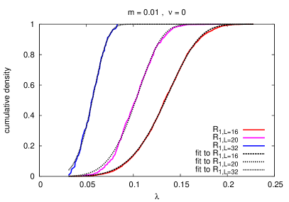
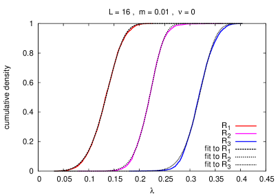
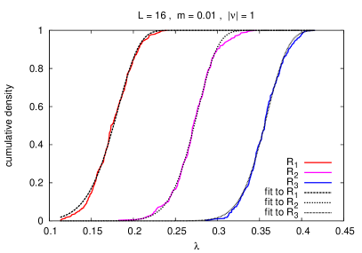
Figure 1: Cumulative Dirac eigenvalue densities at $m=0.01$, and the fitted Kovács distributions (3). We show above the leading eigenvalue in the topologically neutral sector ($\nu=0$) and lattice sizes $L=16,\ 20,\ 32$. Below we refer to $L=16$ and include the leading three non-zero eigenvalues in the sectors $|\nu|=0$ and $1$.

Next we consider the volume dependence of the mean values $\langle\lambda_{n}\rangle$ [11]. We perform fits of the Kovács distribution (3) to these mean values at $m=0.01$, in volumes $V=16^{2}\dots 32^{2}$. Figure 2 shows that also these fits work quite well. The plot on the left illustrates the $V$-dependence of $\langle\lambda_{1}\rangle$ in the sector $|\nu|=1$; the fit (bold line) matches the data in four volumes practically within the errors. The plot on the right extends this consideration to $n=1\dots 4$: all four eigenvalues in four volumes are captured well by adjusting the two parameters $c$ and $\alpha$ in the ansatz (1).

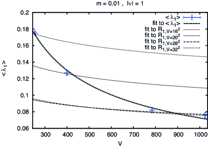
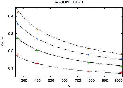
Figure 2: The volume dependence of the mean values $\langle\lambda_{n}\rangle$. The plot on the left (right) shows the data for $\langle\lambda_{1}\rangle$ (for $\langle\lambda_{1}\rangle\dots\langle\lambda_{4}\rangle\,$) in four volumes, which agree quite well with the $V$ dependent Kovács distributions (3), if we fit the free parameters $\alpha$ and $c$. However, the values of the fit parameters differ strongly from those required in Figure 1, which adjust the detailed distribution in one volume. These parameter sets correspond to the four finer lines in the plot on the left.

So far this seems to confirm that our microscopic Dirac spectra are compatible with the decorrelation property. However, each fit in Figure 1 was performed by tuning the two free parameters independently. In Figure 2 they were adjusted again, now to the expected volume dependence. The consistency condition is that the values of these parameters should be compatible, in particular the (dimensionless) exponent $\alpha$.

This is not the case: the $\alpha$ values required for these fits vary between $0.58(3)$ and $8.08(5)$ (and the coefficient $c$ even varies from $0.09(3)$ to $2.7(2)\cdot 10^{4}$) [11]. For a graphical illustration, the plot on the left of Figure 2 also shows lines for the parameter sets which were chosen in Figure 1 for the detailed distribution in each volume. We see that these lines are far from the mean values in distinct volumes. Therefore, the agreement cannot be confirmed, although it is amazing that the single fits work so well.

As a compelling test, we now focus on the distribution of the unfolded level spacings $s$ (which is described e.g. in Refs. [9, 10]). We saw in Ref. [9] that the entire Dirac spectrum follows very precisely the behaviour, which was predicted for the Chiral Unitary Ensemble (ChUE) [12]

$$\rho_{\rm ChUE}(s)=32\Big{(}\frac{s}{\pi}\Big{)}^{2}\exp(-4s^{2}/\pi)\ ,$$ (6)

just like QCD in the $\epsilon$-regime [10]. On the other hand, Ref. [13] observed in high temperature QCD with $2+1$ flavours a transition to a Poisson distribution $\rho_{\rm Poisson}(s)=\exp(-s)$, if one only includes low lying eigenvalues.

Hence we test specifically the unfolded level spacing density for the lowest two Dirac eigenvalues of each configuration [11]. Figure 3 shows the results for $m=0.01$, $\nu=0$ and $L=16$ (on the left), $L=32$ (on the right). In both cases our data are close to the ChUE curve, but far from the Poisson distribution. This is most obvious at $L=16$, where more statistics is included (2428 configurations), while $L=32$ (with 138 configurations) probes smaller eigenvalues.

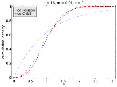
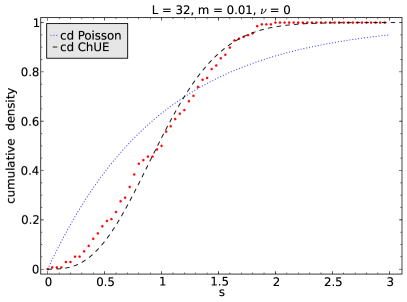
Figure 3: The unfolded level spacing distributions at $m=0.01$, in the topological sector $\nu=0$, for the lowest two Dirac eigenvalues at $L=16$ (on the left) and $L=32$ (on the right). In both cases, our data are compatible with the distribution of a Chiral Unitary Ensemble, but not with a Poisson distribution.

4 Mass anomalous dimension

At last we also take a look at the evaluation of the mass anomalous dimension $\gamma_{m}$. This can be done in various ways; here we follow the procedure which was used in Ref. [14]. As suggested in Ref. [15], it employs the mode number (the cumulative eigenvalue density, up to the normalisation)

$$\nu_{\rm mode}(\lambda)=V\int_{-\lambda}^{\lambda}d\lambda^{\prime}\ \rho(\lambda^{\prime})=\frac{2cV^{2}}{\alpha+1}\ \lambda^{\alpha+1}$$ (7)

as a tool to evaluate the mass anomalous dimension

$$\gamma_{m}(\lambda)=\frac{d}{\alpha(\lambda)+1}-1\ .$$ (8)

We are most interested in its IR limit,

$$\gamma_{m}^{*}=\ ^{~{}\lim}_{\lambda\to 0}\ \gamma_{m}(\lambda)\ .$$ (9)

Figure 4 shows the $\gamma_{m}$ values (which are obtained by averaging over a small interval) for fermion masses $m=0.01$ and $0.06$, in a variety of volumes. In both cases, the data are well compatible with a quadratic fit, which leads to very similar IR extrapolations,

$$m=0.01\ :\ \gamma_{m}^{*}=0.065(5)\ ,\qquad m=0.06\ :\ \gamma_{m}^{*}=0.063(7)\ .$$ (10)

The consistency between these two masses suggests stability of this value in the chiral extrapolation $m\to 0$, and in the large volume extrapolation $L\to\infty$. (Moreover, lattice artifacts are expected to be small, as we mentioned before.)

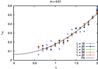
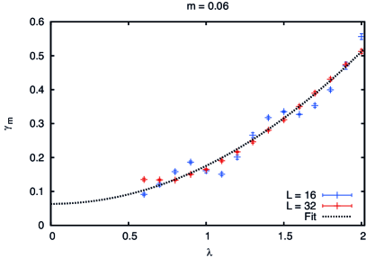
Figure 4: Evaluation of the mass anomalous dimension $\gamma_{m}$ based on the mode number $\nu_{\rm mode}(\lambda)$ at fermion mass $m=0.01$ (on the left) and $m=0.06$ (on the right). The data for both masses lead to very similar IR limits, which are given in eq. (10).

However, this apparently convincing picture is questionable, since the results for $\gamma_{m}^{*}$ depend significantly on the energy interval that we rely on for the extrapolation. Fits to the detailed distributions of the lowest few eigenvalues only lead to $\alpha\simeq 3/5$ [9], which corresponds to $\gamma_{m}^{*}\simeq 1/4$. That value is just between the extreme limits of the HHI parameter,

$$l\ll 1\quad\Rightarrow\quad\gamma_{m}^{*}=0\ ,\qquad l\gg 1\quad\Rightarrow\quad\gamma_{m}^{*}=1/2\ ,$$ (11)

which could be sensible regarding Table 1. In Figure 4 we refer to higher energies, so we are dealing with Dirac eigenvalues closer to the bulk. The corresponding IR extrapolation approaches the non-anomalous value $\gamma_{m}^{*}=0$ of free fermions.

5 Conclusions

We have considered the 2-flavour Schwinger model as a simple fermionic theory with a vanishing chiral condensate in the chiral limit, $\Sigma(m=0)=0$. We started from the hypothesis that in such theories the low lying Dirac eigenvalues could be decorrelated, and therefore Poisson distributed. In fact, this feature had been confirmed for fermions in $d=4$, interacting through Yang-Mills gauge fields at high temperature [4, 13]. However, we could not confirm this property for the 2-flavour Schwinger model. Single fits to the predicted properties work remarkably well — in particular for the density of a specific low eigenvalue — but these fits require parameters, which are clearly inconsistent. Moreover, we saw that the unfolded level spacing distribution for the two lowest eigenvalues of each configuration is close to the form of the Chiral Unitary Ensemble, but far from a Poisson distribution; this coincides with the feature of the entire spectrum.

These observations favour a modified hypothesis: the predicted eigenvalue decorrelation occurs if $\Sigma(m=0)$ vanishes due to high temperature, but not when this happens due to a large number of flavours. In fact, Ref. [17] associates the inverse temperature with the localisation scale for small Dirac eigenvalues, which is fully consistent with this modified hypothesis.

Regarding the mass anomalous dimension $\gamma_{m}$, we found an apparently stable IR extrapolation $\gamma_{m}^{*}$ based on the $\gamma_{m}$ values obtained through the mode number in a moderate spectral regime [11]. However, this result disagrees with fits obtained in the microscopic regime of the lowest Dirac eigenvalues [9]. This underscores once more that $\gamma_{m}^{*}$ is a tricky quantity: different methods may provide apparently convincing values, which still differ significantly. In fact, this is reflected by the recent literature on possibly IR conformal 4d fermionic models (see e.g. Refs. [14, 18]), which is currently one of the most controversial issues in the lattice community.

References

- [1]
- [2] L. Del Debbio, PoS (LATTICE2010) 004.
- [3] A.V. Smilga, Phys. Lett. B 278 (1992) 371, Phys. Rev. D 55 (1997) 443.
- [4] T.G. Kovács, Phys. Rev. Lett. 104 (2010) 031601.
- [5] J.E. Hetrick, Y. Hosotani and S. Iso, Phys. Lett. B 350 (1995) 92.
- [6] H. Leutwyler and A.V. Smilga, Phys. Rev. D 46 (1992) 5607.
- [7] W. Bietenholz, Eur. Phys. J. C 6 (1999) 537, Nucl. Phys. B 644 (2002) 223.
- [8] W. Bietenholz and I. Hip, Nucl. Phys. B 570 (2000) 423.
- [9] W. Bietenholz, I. Hip, S. Shcheredin and J. Volkholz, Eur. Phys. J. C 72 (2012) 1938.
- [10] W. Bietenholz, K. Jansen and S. Shcheredin, JHEP 0307 (2003) 033.
- [11] D. Landa-Marbán, W. Bietenholz and I. Hip, arXiv:1307.0231 [hep-lat].
- [12] M.A. Halasz and J.J.M. Verbaarschot, Phys. Rev. Lett. 74 (1995) 3920.
- [13] T.G. Kovács and F. Pittler, Phys. Rev. D 86 (2012) 114515.
- [14] A. Cheng, A. Hasenfratz, G. Petropoulos and D. Schaich, JHEP 1307 (2013) 061.
- [15] L. Giusti and M. Lüscher, JHEP 0903 (2009) 013.
- [16] Z. Fodor, K. Holland, J. Kuti, D. Nogradi and C. Schroeder, Phys. Lett. B 681 (2009) 353.
- [17] F. Bruckmann, T.G. Kovács and S. Schierenberg, Phys. Rev. D 84 (2011) 034505.
- [18] L. Del Debbio and R. Zwicky, Phys. Rev. D 82 (2010) 014502. A. Cheng, A. Hasenfratz and D. Schaich, Phys. Rev. D 85 (2012) 094509. A. Patella, Phys. Rev. D 86 (2012) 025006. P. de Forcrand, S. Kim and W. Unger, JHEP 1302 (2013) 051. L. Keegan, PoS (LATTICE2012) 044.