Carbon-enhanced Metal-poor Stars in SDSS/SEGUE. I.
Carbon Abundance Estimation and Frequency of CEMP Stars

Abstract

We describe a method for the determination of stellar [C/Fe] abundance ratios using low-resolution ($R=2000$) stellar spectra from the Sloan Digital Sky Survey (SDSS) and its Galactic sub-survey, the Sloan Extension for Galactic Understanding and Exploration (SEGUE). By means of a star-by-star comparison with a set of SDSS/SEGUE spectra with available estimates of [C/Fe] based on published high-resolution analyses, we demonstrate that we can measure [C/Fe] from SDSS/SEGUE spectra with S/N $\geq 15$ Å^-1 to a precision better than 0.35 dex for stars with atmospheric parameters in the range $T_{\rm eff}$ = [4400, 6700] K, $\log~{}g$ = [1.0, 5.0], [Fe/H] = [$-$4.0, $+$0.5], and [C/Fe] = [$-0.25$, $+$3.5]. Using the measured carbon-to-iron abundance ratios obtained by this technique, we derive the frequency of carbon-enhanced stars ([C/Fe] $\geq+0.7$) as a function of [Fe/H], for both the SDSS/SEGUE stars and other samples from the literature. We find that the differential frequency slowly rises from almost zero to about 14% at [Fe/H] $\sim$ –2.4, followed by a sudden increase, by about a factor of three, to 39% from [Fe/H] $\sim$ –2.4 to [Fe/H] $\sim$ –3.7. Although the number of stars known with [Fe/H] $<-4.0$ remains small, the frequency of carbon-enhanced metal-poor (CEMP) stars below this value is around 75%. We also examine how the cumulative frequency of CEMP stars varies across different luminosity classes. The giant sample exhibits a cumulative CEMP frequency of 32% for [Fe/H] $\leq-2.5$, 31% for [Fe/H] $\leq-3.0$, and 33% for [Fe/H] $\leq-3.5$; a roughly constant value. For the main-sequence turnoff stars, we obtain a lower cumulative CEMP frequency, around 10% for [Fe/H] $\leq-2.5$, presumably due to the difficulty of identifying CEMP stars among warmer turnoff stars with weak CH $G$-bands. The dwarf population displays a large change in the cumulative frequency for CEMP stars below [Fe/H] = –2.5, jumping from 15% for [Fe/H] $\leq-2.5$ to about 75% for [Fe/H] $\leq-3.0$. When we impose a restriction with respect to distance from the Galactic mid-plane ($|Z|<5$ kpc), the frequency of the CEMP giants does not increase at low metallicity ([Fe/H] $<-2.5$), but rather, decreases, due to the dilution of C-rich material in stars that have undergone mixing with CNO-processed material from their interiors. The frequency of CEMP stars near the main-sequence turnoff, which are not expected to have experienced mixing, increases for [Fe/H] $\leq-3.0$. The general rise in the global CEMP frequency at low metallicity is likely due to the transition from the inner-halo to the outer-halo stellar populations with declining metallicity and increasing distance from the plane.

1. Introduction

The chemical abundance ratios of very metal-poor (VMP; [Fe/H]$\leq-2.0$) stars in the Milky Way provide vital clues to the early chemical evolution and initial mass function (IMF) of their progenitors, which are likely to have been among the first generations of stars formed in the universe.

Given this importance, there have been increasingly ambitious efforts carried out to identify metal-poor candidates with large-scale surveys of the stellar populations of the Milky Way. The early HK survey (Beers et al. 1985, 1992) and the Hamburg/ESO Survey (HES; Wisotzki et al. 1996; Christlieb 2003; Christlieb et al. 2001, 2008) collectively identified several thousand VMP stars (Beers & Christlieb 2005). In recent years, this number has been dramatically increased by the Sloan Digital Sky Survey (SDSS; Fukugita et al. 1996; Gunn et al. 1998, 2006; York et al. 2000; Stoughton et al. 2002; Abazajian et al. 2003, 2004, 2005, 2009; Pier et al. 2003; Adelman-McCarthy et al. 2006, 2007, 2008; Aihara et al. 2011; Ahn et al. 2012) and the Sloan Extension for Galactic Understanding and Exploration (SEGUE-1; Yanny et al. 2009) and SEGUE-2 (C. Rockosi et al., in preparation), to many tens of thousands of VMP stars. Ongoing surveys, such as Large sky Area Multi-Object fiber Spectroscopic Telescope (LAMOST; Cui et al. 2012; Luo et al. 2012), hold the promise of enlarging this sample to several hundred thousand VMP stars.

Detailed chemical-abundance analyses by a number of groups, based on high-resolution spectroscopic follow-up, have revealed that, while most VMP stars exhibit similar abundance patterns, there are numerous examples of objects with peculiar chemical patterns, such as strong enrichments or deficiencies of light elements such as C, N, O, Na, Mg, Si, etc. (e.g., McWilliam et al. 1995; Ryan et al. 1996; Norris et al. 2001, 2013; Johnson 2002; Cayrel et al. 2004; Aoki et al. 2008, 2013; Cohen et al. 2008; Lai et al. 2008). Frebel & Norris (2012) provide a useful summary of all but the most recent work. Among the chemically peculiar stars with [Fe/H] $\leq-2.0$, objects with enhanced carbon abundance are the most common variety.

The carbon-enhancement phenomenon was recognized over a half century ago for stars with [Fe/H] $\sim$ –2.0 to [Fe/H] $\sim-1.0$. Such objects were called CH stars (Keenan 1942) or subgiant CH stars (Bond 1974), because their optical spectra exhibit strong CH $G$-band absorption features around 4300 Å compared to stars with similar effective temperatures and metallicities. Over the past quarter century, spectroscopic follow-up of metal-poor candidates selected from the HK and HES surveys have identified many more such stars at even lower metallicity (e.g., Beers et al. 1985, 1992; Christlieb et al. 2001; Christlieb 2003). These stars are referred to as carbon-enhanced metal-poor (CEMP) stars, originally defined as having metallicity [Fe/H] $\leq-1.0$ and carbon-to-iron ratios larger than 10 times the solar ratio (i.e., [C/Fe] $>+1.0$; Beers & Christlieb 2005); definitions of CEMP stars using the criteria [C/Fe] $>+0.5$ and [C/Fe] $>+0.7$ have also been employed by a number of authors (e.g., Aoki et al. 2007).

Recent studies of VMP stars discovered from various spectroscopic surveys have confirmed that the cumulative fraction of CEMP stars strongly increases with decreasing metallicity. Overall, the cumulative fraction of CEMP stars rises from $\sim$ 20 % for [Fe/H] $<-2.0$, 30% for [Fe/H] $<-3.0$, 40% for [Fe/H] $<-3.5$, and 75% for [Fe/H] $<-4.0$, after the inclusion of a carbon-normal star with [Fe/H] $\sim-5.0$ (Beers & Christlieb 2005; Marsteller et al. 2005; Rossi et al. 2005; Frebel et al. 2006; Lucatello et al. 2006; Norris et al. 2007, 2013; Carollo et al. 2012; Spite et al. 2013; Yong et al. 2013).

The high frequency of CEMP stars at low metallicity indicates that a large amount of carbon (relative to iron) was produced at an early evolutionary stage of the Milky Way. Other evidence for the large production of carbon at early times comes from the discovery by Cooke et al. (2011) of an extremely metal-poor (EMP; [Fe/H] $\sim–3.0$) damped Ly-$\alpha$ (DLA) system at $z=2.3$ that exhibits enhanced a carbon abundance ratio ([C/Fe]$=+1.5$) and other elemental-abundance signatures similar to the CEMP-no class of stars. This classification (defined by Beers & Christlieb 2005) describes CEMP stars with no strong enhancements of $s$-process elements. Matsuoka et al. (2011) also reported evidence for strong carbon production in the early universe, based on their analysis of the optical spectrum of the most distant known radio galaxy, with $z$ = 5.19.

The mechanisms that have been proposed to account for this large carbon production include: (1) mass transfer of carbon-enhanced material from the envelope of an asymptotic giant branch (AGB) star to its (presently observed) binary companion (e.g., Herwig 2005; Sneden et al. 2008; Masseron et al. 2010; Bisterzo et al. 2011, 2012); (2) massive, rapidly rotating, zero-metallicity stars, which produce large amounts of carbon, nitrogen, and oxygen due to distinctive internal burning and mixing episodes (Meynet et al. 2006, 2010); and (3) faint supernovae associated with the first generations of stars, which experience extensive mixing and fallback during their explosions and eject large amounts of C and O (Umeda & Nomoto 2003, 2005; Tominaga et al. 2007; Ito et al. 2009, 2013).

This early carbon production can have a profound influence on the chemical evolution of the Galaxy and the universe. As argued by Abia et al. (2001) and Lucatello et al. (2005), and most recently by Suda et al. (2013), the large fraction of CEMP stars at the lowest metallicities could indicate that the IMF in the early universe included a larger number of intermediate- to high-mass stars than the present-day IMF. However, Izzard et al. (2009) and Abate et al. (2013), using a binary population model alone, could not reproduce the high fraction of CEMP stars among the most metal-poor stars.

In order to understand the carbon-enhanced phenomenon among low-metallicity stars, there have been a number of efforts to estimate carbon abundance from low- and medium-resolution stellar spectroscopic surveys of metal-poor candidates. Generally, these efforts were limited in terms of sample size, coverage of stellar parameter space, and methodology for determining [C/Fe]. For example, the early approach of Rossi et al. (2005) made use of the strength of the Ca ii K line and CH $G$-band, along with the associated broadband $J-K$ colors, to estimate [Fe/H] and [C/Fe] for medium-resolution (1–2 Å) spectra of HK-survey stars. Frebel et al. (2006) followed Rossi et al.’s prescription to obtain [C/Fe] for a subset of 234 stars among 1777 metal-poor candidates from the HES survey, deriving a frequency of 9%$\pm$2% for VMP giants with [C/Fe] $>+1.0$. Very recently, Carollo et al. (2012) employed a grid of synthetic spectra, covering a wide range of parameter space, in order to match with the SDSS/SEGUE stellar spectra around the CH $G$-band region to derive the carbon-to-iron ratios. They applied their technique to the calibration stars (used for spectrophotometric corrections and tests of interstellar reddening) from SDSS/SEGUE, ending up with about 31,000 stars with derived carbon abundances (or upper limits), the largest previous effort to measure [C/Fe] for halo stars to date.

The SDSS/SEGUE surveys have produced an unprecedented sample of stellar spectra for more detailed analysis. SEGUE-1 was one of three sub-surveys comprising SDSS-II (Legacy, Supernova Survey, and SEGUE-1). The SEGUE-1 program obtained $ugriz$ imaging of some 3500 deg² of sky outside of the original SDSS footprint, and roughly 240,000 low-resolution ($R=2000$) stellar spectra covering the wavelength range 3820–9100 Å. SEGUE-2, executed during an early stage of the ongoing SDSS-III effort, observed stars fainter than the SEGUE-1 survey, and added an additional $\sim$140,000 stars. Stellar spectra obtained as calibration objects or ancillary projects during regular SDSS-I and SDSS-II operations account for roughly another 200,000 stars, yielding a total of about 600,000 stars potentially suitable for further analysis. For simplicity, we refer to all of the SDSS, SEGUE-1, and SEGUE-2 stellar spectra to as SDSS/SEGUE spectra (stars) throughout this paper.

Since this stellar database includes stars in many evolutionary stages and spans a wide range of metallicity ($-4.0<$ [Fe/H] $<+0.5$), measurement of the carbon-to-iron ratios enables the determination of the frequency of the CEMP phenomenon for stars of various spectral types, luminosity classes, and metallicities. This should, in turn, provide valuable constraints on Galactic chemical evolution models, numerical simulations of Galaxy formation, the nature of the IMF at early times, and the various proposed carbon-production mechanisms.

In this paper, we present new techniques for the measurement of [C/Fe], and derive the frequency of CEMP stars from the large sample of SDSS/SEGUE spectra. Section 2 describes our methodology for estimation of [C/Fe]. A validation of this method, based on a star-by-star comparison with high-resolution spectroscopy of SDSS/SEGUE stars in the literature, is provided in Section 3. The impact of signal-to-noise ratios (S/Ns) on the measured [C/Fe] is also examined in Section 3. Section 4 derives the frequency of the CEMP stars, as a function of [Fe/H], for the full sample, as well as for stars in various luminosity classes. A summary of our results and our conclusions are provided in Section 5.

2. Measurement of Carbon-to-Iron Ratios ([C/Fe])

2.1. Stellar Atmospheric Parameters

In order to derive the fundamental stellar atmospheric parameters ($T_{\rm eff}$, $\log~{}g$, and [Fe/H]) for the SDSS/SEGUE spectra, we employ the most recent update of the SEGUE Stellar Parameter Pipeline (SSPP; Lee et al. 2008a, 2008b, 2011; Allende Prieto et al. 2008; Smolinski et al. 2011). The SSPP processes the wavelength- and flux-calibrated SDSS/SEGUE stellar spectra, and delivers the three fundamental stellar parameters for most stars with spectral S/N ratio greater than 10 Å^-1, in the temperature range 4000–10,000 K. The SSPP estimates the atmospheric parameters through a number of approaches, such as a minimum distance method (Allende Prieto et al. 2006), neural network analysis (Bailer-Jones 2000; Re Fiorentin et al. 2007), and a variety of line-index calculations, which were calibrated with respect to known standard stars (e.g., Beers et al. 1999). This multiple approach permits the use of as wide a spectral range as possible, in order for the SSPP to obtain robust estimates of each parameter for stars over a wide range in $T_{\rm eff}$, $\log~{}g$, [Fe/H], and S/N. The SSPP is able to determine $T_{\rm eff}$, $\log~{}g$, and [Fe/H] with typical external errors of 180 K, 0.24 dex, and 0.23 dex, respectively (Smolinski et al. 2011), most reliably for stars in the temperature range 4500 K $<$ $T_{\rm eff}$ $<$ 7500 K. As described by Lee et al. (2011), the SSPP can also obtain an estimate of [$\alpha$/Fe], with a precision of better than 0.1 dex, for SDSS/SEGUE spectra having S/N $\geq 20$ Å^-1.

2.2. A New Grid of Synthetic Spectra for Determination of [C/Fe]

Since it is not practical to analyze hundreds of thousands of stellar spectra one at a time, we have modified the SSPP so that it is capable of estimating [C/Fe] in a fast, efficient manner. To accomplish this, we introduce a pre-existing grid of synthetic spectra. This eliminates the need for generating synthetic spectra on the fly, while simultaneously attempting to determine the primary atmospheric parameters and/or other elemental abundances.

As emphasized in Masseron (2006), carbon enhancement affects the thermodynamical structure of stellar atmospheres. To take into account this effect, specific models have been tailored with various carbon abundances using the MARCS code (Gustafsson et al. 2008). From those models, we have created synthetic spectra using the Turbospectrum synthesis code (Alvarez & Plez 1998; Plez 2012), which employs the line broadening treatment described by Barklem & O’Mara (1998), along with the solar abundances of Asplund et al. (2005). The sources of atomic lines used by Turbospectrum come from VALD (Kupka et al. 1999), Hill et al. (2002), and Masseron (2006). Line-lists for the molecular species are provided for CH (T. Masseron et al., in preparation), and CN and C₂ (B. Plez, private communication); the lines of MgH molecules are adopted from the Kurucz linelists.

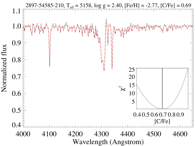
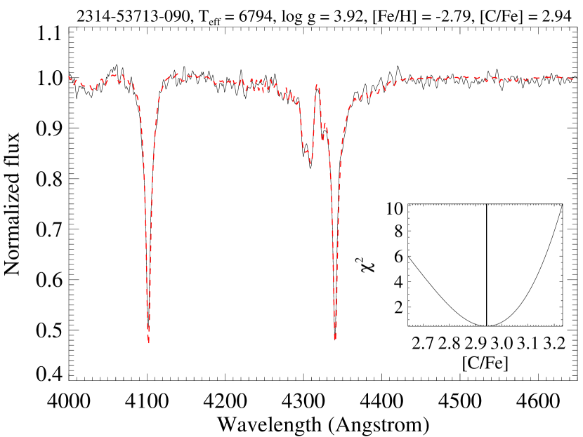
Figure 1.— Two examples of our spectral matching technique, illustrating clear detections of the CH $G$-band. The left panel is a cool, VMP, moderately carbon-enhanced giant ([C/Fe] $=+0.69$), whereas the right panel exhibits a warm, VMP, highly carbon-enhanced turnoff star ([C/Fe] $=+2.94$). The black line is the observed spectrum, while the red-dashed line is the best-matching synthetic spectrum generated with the parameters listed on each plot, as estimated by our approach and the SSPP. The inset plot in each panel shows the change of the $\chi^{2}$ values over [C/Fe] around the adopted [C/Fe]. The solid vertical line indicates the measured [C/Fe] at the minimum of $\chi^{2}$.

When synthesizing the spectra, we increase (by the same amount) the abundances for the $\alpha$-elements (O, Mg, Si, Ca, and Ti). We assume that the $\alpha$-enhancement ratio, relative to Fe, is $+$0.4 for [Fe/H] $\leq-1.0$, $+$0.2 for [Fe/H] = $-0.5$, and 0.0 for [Fe/H] $\geq 0.0$. As it is often found that N is enhanced in CEMP stars (Masseron et al. 2010), we assume the same level of N enhancement as for carbon (i.e., [N/Fe] = [C/Fe]). We also assumed a carbon isotopic composition of ¹²C/¹³C = 10. We do not consider any neutron-capture element enhancements (which in any case would have a small effect on spectra at the resolution of SDSS/SEGUE). In order to assign an appropriate microturbulence velocity ($\xi_{t}$) for each spectrum, we make use of a simple polynomial relationship between microturbulence velocity and surface gravity, $\xi_{t}$ [km s^-1] = $-0.345\cdot$log $g+2.225$, derived from the high-resolution spectra of SDSS/SEGUE stars used to calibrate the SSPP. The synthetic spectra have wavelength steps of 0.01 Å, covering the wavelength range 4000–5000 Å, which includes the CH $G$-band ($\sim$4300 Å), as well as lines of Sr ii ($\sim$4077 Å) and Ba ii ($\sim$4554 Å).

The final grid covers 4000 K $\leq T_{\rm eff}\leq$ 7000 K in steps of 250 K, 1.0 $\leq\log~{}g\leq$ 5.0 in steps of 0.5 dex, and $-4.0\leq\rm[Fe/H]\leq+0.5$ in steps of 0.25 dex. The range of [C/Fe] varies with the metallicity in steps of 0.25 dex as follows:

• $-0.5\leq$ [C/Fe] $\leq+3.5$ for [Fe/H] $\leq-1.25$

• $-0.5\leq$ [C/Fe] $\leq+1.5$ for $-1.25<$ [Fe/H] $\leq-0.75$

• $-0.5\leq$ [C/Fe] $\leq+1.0$ for [Fe/H] $>-0.75$

The total number of generated synthetic spectra is 30,069. Once created, the full set of synthetic spectra are degraded to SDSS resolution ($R=2000$), and re-sampled to 1 Å wide linear pixels over the wavelength 4000–4650 Å. Each degraded grid is normalized by division with a pseudo continuum, obtained by the same continuum-fitting routine used for the observed spectra.

2.3. Determination of [C/Fe]

In order to determine [C/Fe] for the SDSS/SEGUE spectra, we first transform the vacuum wavelength scale to an air-based scale, and shift the spectrum to the rest frame using a measured radial velocity. This wavelength and redshift-corrected spectrum is linearly re-binned to 1 Å pixels over the wavelength range 4000–4650 Å, in which the CH $G$-band is included. When pre-processing the synthetic spectra, the spectrum under consideration is then normalized by dividing its reported flux by its pseudo-continuum.

The pseudo-continuum over the 4000–4650 Å range is obtained by carrying out an iterative procedure that rejects points lying more than 1$\sigma$ below and 4$\sigma$ above the fitted function, obtained from a ninth-order polynomial. Although we have a “perfect” continuum available for a given synthetic spectrum, we apply the same continuum routine to the synthetic and SDSS spectra to match with over the same wavelength range, and with the same pixel size. Application of the same continuum routine produces the same level of line-strength suppression in both spectra.

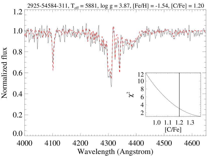
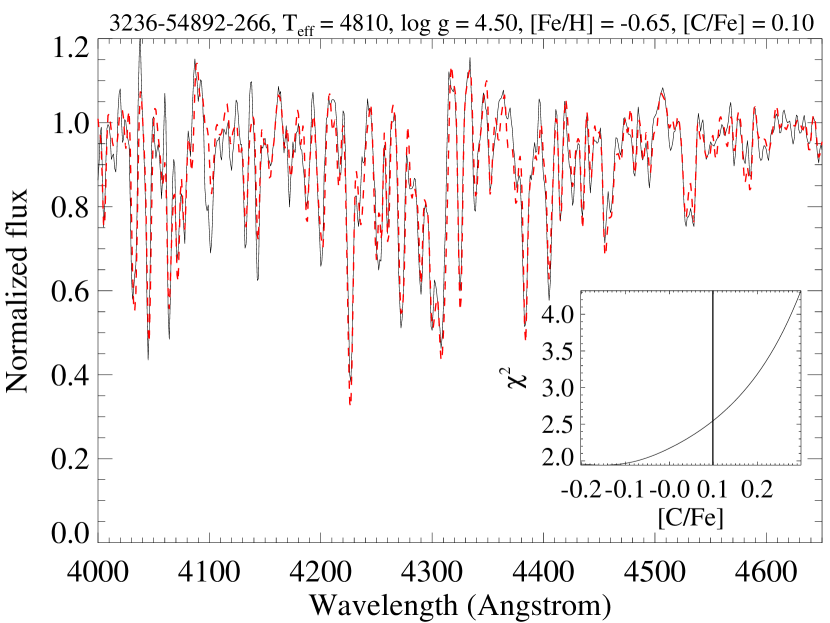
Figure 2.— Two examples of a lower limit (left panel) and upper limit (right panel) on estimates of [C/Fe] from our spectral matching technique. The spectrum shown in the left panel is a carbon-enhanced ([C/Fe] $=+1.20$), metal-poor star, while the right panel is a typical, carbon-normal ([C/Fe] = $+0.10$) thick-disk dwarf star. The black line is the observed spectrum, while the red-dashed line is the best-matching synthetic spectrum generated with the parameters listed on each plot, as determined by our methodology and the SSPP. The inset plot in each panel exhibits the change of $\chi^{2}$ versus [C/Fe]. The solid vertical line in each panel is where the lower or upper limit is determined (which is not at the minimum of $\chi^{2}$ values, see text).

Following the above steps, we then search the grid of synthetic spectra for the best-fitting model parameters by minimizing the distance between the normalized target and synthetic flux, using a reduced $\chi^{2}$ statistical criterion. The parameter search over the grid is carried out by the IDL function minimization routine MPFIT (Markwardt 2009). In this search, we fix $T_{\rm eff}$ and $\log~{}g$ to the value determined (previously) by the SSPP, and change [Fe/H] and [C/Fe] simultaneously to generate a trial model spectrum by spline interpolation from the existing grid, rather than vary all four parameters at once. Since the temperature has the greatest influence on the spectral features over the wavelength range we consider, holding it constant permits the more subtle variations associated with the other parameters to be explored. We also find that the metallicity has a greater impact on measuring [C/Fe] than the surface gravity. Therefore, we allow [Fe/H] to vary, but not $\log~{}g$. The errors in [Fe/H] and [C/Fe] estimated by this approach are determined by the square root of diagonal elements of the resulting covariance matrix.

Even though the $\chi^{2}$ minimization approach reproduces [C/Fe] well, we seek to improve the accuracy of the carbon measurement so that there are not spurious detections of carbon-rich stars. Thus, we include an additional step to check on the estimated [C/Fe]. Briefly, at a given $T_{\rm eff}$, $\log~{}g$, and [Fe/H] (this metallicity estimate is determined from the above $\chi^{2}$ minimization), we generate by interpolation a series of synthetic spectra by varying [C/Fe] by 0.01 dex, from –1.0 to $+$1.0 dex from the above determined value over the spectral range 4290–4318 Å (in which the prominent CH $G$-band feature exists), and check how the $\chi^{2}$ values from the differences between the synthetic spectra and the observed spectrum change. We fit a spline function to the distribution of the $\chi^{2}$ values against [C/Fe], in order to establish the local minimum point where [C/Fe] is determined. We demand that the extrema of the $\chi^{2}$ values are at least 10% above the local minimum. In this case, we raise a ‘D’ flag, indicative of a clear detection of CH $G$-band.

In cases where no minimum is found, the $\chi^{2}$ behavior typically reveals a continuously declining trend of $\chi^{2}$ toward the edge of the grid. We fit to the portion of the declining function of $\chi^{2}$ with a Gaussian function having a mean value of [C/Fe] at the minimum of declining $\chi^{2}$, in order to estimate the full width half maximum (FWHM) of this variation. After adding (subtracting) the FWHM to (from) the [C/Fe] value found at the minimum of the declining $\chi^{2}$, we conservatively define the value as the upper (lower) limit of the measured [C/Fe], depending at which edge of the grid the minimum is found. Accordingly, we raise an ‘L’ flag for a lower limit and a ‘U’ flag for an upper limit. In this way, we can ensure to have a clear measurement of the upper or lower limit on [C/Fe], rather than a spurious estimate of [C/Fe] that can occur in the very low-metallicity (and/or high $T_{\rm eff}$) regime, due to the weakness of the CH $G$-band.

It is worth mentioning that the [C/Fe] values determined by this approach agree well with the estimates from the $\chi^{2}$ minimization technique. We find in most cases small mean offsets ($<0.05$ dex) and scatter ($<0.1$ dex) between the two approaches.

Figure 1 provides two examples of clear detections of the CH $G$-band by our spectral fitting method. The left panel is a cool, VMP, moderately carbon-enhanced giant ([C/Fe] $=+0.69$), while the right panel shows a warm, VMP, highly carbon-enhanced turnoff star ([C/Fe] $=+2.94$). The black line is the observed spectrum; the red-dashed line is the best-matching synthetic spectrum generated with the parameters listed at the top of each plot, as determined by our methodology and the SSPP. The inset plot in each panel displays how the $\chi^{2}$ values over 4290–4318 Å change with [C/Fe] around the adopted [C/Fe], the vertical solid line. From inspection, one can see that an excellent match between the synthetic and observed spectra is achieved for these two stars.

Figure 2 shows examples of spectra with a lower limit (left panel) and upper limit (right panel) on [C/Fe] obtained following the technique described above. The spectrum in the left panel is a carbon-enhanced, metal-poor star, while the right panel is a typical thick-disk dwarf star. The layout of the figure is the same as for Figure 1. The inset plots display continuously declining or increasing values of $\chi^{2}$ over [C/Fe]. The solid vertical line in each panel indicates where the lower or upper limit is determined from the above prescription (which is clearly not at the minimum of $\chi^{2}$ values). As seen in the figure, a lower limit of [C/Fe] $=+1.20$ for the star in the left panel indicates that it is a highly C-enhanced star, while the upper limit of [C/Fe] $=+0.10$ for the star in the right panel implies that it is a C-normal star.

Table 1Adopted Atmospheric Parameters and [C/Fe] of the SSPP and High-resolution Calibration Samples

SDSS Plate–		High Resolution					SSPP
MJD–Fiber	IAU Name	$T_{\rm eff}$	$\log~{}g$	[Fe/H]	[C/Fe]	$\sigma_{\rm[C/Fe]}$	$T_{\rm eff}$	$\log~{}g$	[Fe/H]	[C/Fe]	$\sigma_{\rm[C/Fe]}$	S/N	Ref.
		(K)	(dex)	(dex)	(dex)	(dex)	(K)	(dex)	(dex)	(dex)	(dex)
0304-51609-528	SDSS J142237.43$+$003105.2	5200	2.20	$-$3.03	$+$1.70	0.14	5361	2.76	$-$3.08	$+$1.98	0.26	44	A13
0353-51703-195	SDSS J170733.93$+$585059.7	6700	4.20	$-$2.52	$+$2.10	0.32	6579	3.40	$-$2.36	$+$2.20	0.25	62	A08
0471-51924-613	SDSS J091243.72$+$021623.7	6150	4.00	$-$2.68	$+$2.05	0.22	6211	3.38	$-$2.64	$+$2.44	0.25	59	A13
0654-52146-011	SDSS J003602.17$-$104336.3	6500	4.50	$-$2.41	$+$2.32	0.32	6476	3.59	$-$2.72	$+$2.87	0.30	44	A08
0913-52433-073	SDSS J134913.54$-$022942.8	6200	4.00	$-$3.24	$+$3.01	0.22	6182	3.14	$-$3.04	$+$3.27	0.29	40	A13
0938-52708-608	SDSS J092401.85$+$405928.7	6200	4.00	$-$2.51	$+$2.72	0.32	6239	3.31	$-$2.25	$+$2.65	0.28	46	A08
0982-52466-480	SDSS J204728.85$+$001553.8	6600	4.50	$-$2.05	$+$2.00	0.32	6317	3.52	$-$2.13	$+$1.93	0.25	47	A08
1213-52972-507	SDSS J091849.91$+$374426.6	6463	4.34	$-$2.98	$+$2.82	$\cdots$	6418	3.41	$-$3.07	$+$3.34	0.27	45	Y13
1266-52709-432	SDSS J081754.93$+$264103.8	6300	4.00	$-$3.16	$<+$2.20	$\cdots$	6111	3.28	$-$2.85	$+$1.31	0.26	43	A08
1475-52903-110	SDSS J220924.74$-$002859.8	6200	4.00	$-$3.96	$+$2.56	$\cdots$	6539	3.55	$-$2.87	$+$2.44	0.28	15	S13
1489-52991-251	SDSS J235718.91$-$005247.8	5200	4.80	$-$3.20	$+$0.57	0.22	5196	3.65	$-$3.34	$+$0.82	0.25	53	A13
1513-53741-338	SDSS J025956.45$+$005713.3	4550	5.00	$-$3.31	$-$0.02	0.22	4679	4.15	$-$3.05	$-$0.00	0.25	43	A13
1600-53090-378	SDSS J103649.93$+$121219.8	5850	4.00	$-$3.47	$+$1.84	0.22	5949	3.19	$-$2.82	$+$1.55	0.28	46	A13
1690-53475-323	SDSS J164610.19$+$282422.2	6100	4.00	$-$3.05	$+$2.52	0.22	6160	3.14	$-$2.61	$+$2.69	0.25	44	A13
1996-53436-093	SDSS J112813.57$+$384148.9	6449	4.38	$-$3.53	$<+$1.66	$\cdots$	6629	3.55	$-$2.80	$+$0.87	0.52	45	Y13
2044-53327-515	SDSS J014036.22$+$234458.1	5703	3.36	$-$4.09	$+$1.57	$\cdots$	6155	3.51	$-$3.64	$+$2.03	0.26	56	Y13
2176-54243-614	SDSS J161313.53$+$530909.7	5350	2.10	$-$3.33	$+$2.09	0.14	5469	2.79	$-$2.71	$+$1.81	0.25	51	A13
2178-54629-546	SDSS J161226.18$+$042146.6	5350	3.30	$-$2.86	$+$0.63	0.14	5418	2.58	$-$2.60	$+$0.39	0.25	43	A13
2183-53536-175	SDSS J174624.13$+$245548.8	5350	2.60	$-$3.17	$+$1.24	0.14	5378	2.47	$-$2.59	$+$0.56	0.24	48	A13
2202-53566-537	SDSS J162603.61$+$145844.3	6400	4.00	$-$2.99	$+$2.86	0.22	6410	3.37	$-$2.46	$+$2.65	0.27	41	A13
2309-54441-290	SDSS J220646.20$-$092545.7	5100	2.10	$-$3.17	$+$0.64	0.14	5167	2.12	$-$2.94	$+$0.50	0.24	55	A13
2314-53713-090	SDSS J012617.95$+$060724.8	6900	4.00	$-$3.01	$+$3.08	0.22	6794	3.92	$-$2.79	$+$2.94	0.24	52	A13
2335-53730-314	SDSS J030839.27$+$050534.9	5950	4.00	$-$2.19	$+$2.36	0.22	6013	3.19	$-$2.18	$+$2.44	0.25	41	A13
2337-53740-564	SDSS J071105.43$+$670228.2	5350	3.00	$-$2.91	$+$1.98	0.14	5421	2.32	$-$2.67	$+$2.22	0.25	53	A13
2380-53759-094	SDSS J085833.35$+$354127.3	5200	2.50	$-$2.53	$+$0.30	0.14	5167	2.03	$-$2.68	$+$0.49	0.25	55	A13
2506-54179-576	SDSS J114323.43$+$202058.1	6240	4.00	$-$3.15	$+$2.75	$\cdots$	6292	3.29	$-$3.28	$+$3.36	0.25	41	S13
2540-54110-062	SDSS J062947.45$+$830328.6	5550	4.00	$-$2.82	$+$2.09	0.22	5706	3.01	$-$2.37	$+$2.45	0.25	46	A13
2552-54632-090	SDSS J183601.71$+$631727.4	5350	3.00	$-$2.85	$+$2.02	0.14	5361	2.40	$-$3.09	$+$2.76	0.27	55	A13
2667-54142-094	SDSS J085136.68$+$101803.2	6456	3.87	$-$2.96	$<+$1.39	$\cdots$	6484	3.53	$-$2.95	$+$0.85	0.27	41	Y13
2679-54368-543	SDSS J035111.27$+$102643.2	5450	3.60	$-$3.18	$+$1.55	0.14	5631	2.93	$-$2.77	$+$1.81	0.24	53	A13
2689-54149-292	SDSS J124123.93$-$083725.5	5150	2.50	$-$2.73	$+$0.50	0.14	5231	2.90	$-$2.49	$+$0.67	0.25	57	A13
2689-54149-491	SDSS J124502.68$-$073847.1	6100	4.00	$-$3.17	$+$2.53	0.22	6224	3.02	$-$2.47	$+$2.67	0.32	41	A13
2799-54368-138	SDSS J173417.89$+$431606.5	5200	2.70	$-$2.51	$+$1.78	0.14	5421	2.12	$-$2.75	$+$2.55	0.29	45	A13
2803-54368-459	SDSS J000219.87$+$292851.8	6150	4.00	$-$3.26	$+$2.63	0.22	6248	3.47	$-$2.76	$+$2.64	0.25	81	A13
2808-54524-510	SDSS J170339.60$+$283649.9	5100	4.80	$-$3.21	$+$0.28	0.22	5136	3.98	$-$3.10	$+$0.32	0.25	82	A13
2857-54453-245	SDSS J111407.08$+$182831.8	6200	4.00	$-$3.35	$+$3.25	$\cdots$	6273	3.56	$-$3.22	$+$3.25	0.26	42	S13
2897-54585-210	SDSS J124204.43$-$033618.1	5150	2.50	$-$2.77	$+$0.64	0.14	5158	2.40	$-$2.77	$+$0.69	0.24	61	A13
2939-54515-414	SDSS J074104.22$+$670801.7	5200	2.50	$-$2.87	$+$0.74	0.14	5266	1.99	$-$2.77	$+$1.05	0.25	89	A13
2941-54507-222	SDSS J072352.21$+$363757.2	5150	2.20	$-$3.32	$+$1.79	0.14	5300	2.33	$-$3.20	$+$2.10	0.26	59	A13

Note. — In column labeled Ref. the references are as follows. A08: Aoki et al. (2008); A13: Aoki et al. (2013); Y13: Yong et al. (2013); S13: Spite et al. 2013. Note that the stars SDSS J081754.93$+$264103.8, SDSS J112813.57$+$384148.9, and SDSS J085136.68$+$101803.2 have only reported upper limits on [C/Fe]. S/N is the average signal-to-noise ratio per Angstrom between 4000 and 8000 Å of the SDSS/SEGUE spectrum. The error estimate of the SSPP [C/Fe] follows from application of Equation1 (1) and (2).

3. Validation of the [C/Fe] Determinations

3.1. Star-by-star Comparison with High-resolution Abundance Analysis

Having developed a new technique for the estimation of [C/Fe], we now seek to calibrate and validate this method with external measurements. Although this can be carried out by comparison with the overall behavior of a sample of stars, it is preferable to compare star-by-star (ideally against different sources of external measurements), in order to quantify possible systematic offsets (and optionally remove them), as well as to determine the likely external errors associated with the estimate. For these purposes, we employ a set of SDSS/SEGUE stars with available high-resolution spectroscopy analyzed by Aoki et al. (2008, 2013), Spite et al. (2013), and Yong et al. (2013). Table 1 lists the stars used to validate our technique, along with their adopted atmospheric parameters from the high-resolution spectra, and those used by the SSPP.

The majority of the stars in Table 1 were analyzed by Aoki et al. (2008, 2013), who obtained high-dispersion ($R\sim 36,000$) spectra with the Subaru Telescope High Dispersion Spectrograph (Noguchi et al. 2002). The four stars listed from Yong et al. (2013) were observed with Keck/HIRES at $R=48,000$. The spectra for the three stars from Spite et al. (2013) were collected with VLT/UVES (Dekker et al. 2000) at a resolving power of $R\sim 39,000$. Note that, depending on the adopted model atmospheres, abundance scales, and different effective temperature scales in the analyses of the high-resolution spectra, there could be some systematic offsets between these three sets of analyses. However, we expect any such offsets to be small, and therefore do not attempt to correct for them here.

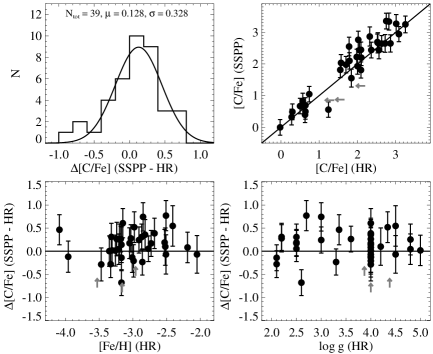
Figure 3.— Comparisons of our measured carbon abundances (SSPP) with those from the literature values based on high-resolution spectroscopy (HR), as listed in Table 1. A systematic offset of 0.128 dex, with a standard deviation of 0.328 dex, is noted from the Gaussian fit to the differences between the two estimates shown in the upper-left panel. The left-pointing arrows in the upper-right panel, and the upward pointing arrows in the lower two panels, indicate upper limit estimates on [C/Fe] delivered from the literature (they are reported as detections with lower values from the SSPP). The error bars in the two lower panels are obtained from the quadratic addition of our measured total error to the literature error, while the error bars in the upper-right panel are the total errors computed from application of Equation (2).

One limitation of this comparison sample is that, as noted from inspection of the table, the sample consists of mainly main-sequence turnoff stars with [Fe/H] $<-2.0$; hence it does not cover a wide range of $T_{\rm eff}$ and [Fe/H]. Nevertheless, since it is more important to obtain accurate [C/Fe] estimates for metal-poor stars than metal-rich stars, it should still serve as an excellent sample to test how well our method performs in the low-metallicity regime.

Figure 3 illustrates a comparison of our measured carbon-abundance ratios with the adopted literature values based on high-resolution abundance analyses. The notation “SSPP” refers to the analysis of the low-resolution SDSS/SEGUE spectra, while “HR” denotes the high-resolution determination. An average systematic offset of 0.128 dex, with a standard deviation of 0.328 dex, is noticed from the Gaussian fit to the residuals (SSPP$-$HR) between the two estimates, shown in the upper-left panel. Note that this offset is not unexpected, given the use of our improved carbon-enhanced model atmospheres (carbon-enhanced models are not used in most high-resolution abundance analyses due to the difficulty of generating such models), and the different molecular linelists employed by the high-resolution analyses. As the offset is small, and in any case much lower than the rms scatter, we do not attempt to adjust our measurements. There are also no strong trends with either [Fe/H] or $\log~{}g$, as shown in the lower panels. The left-pointing arrows in the upper-right panel, and the upward pointing arrows in the lower two panels, indicate upper limit estimates on [C/Fe] drawn from the literature (they are reported as detections with lower values from the SSPP).

As the uncertainty in our measured [C/Fe] includes both external and internal random errors, and the abundances that we employ from the literature (based on the high-resolution analyses) carries its own errors as well, we quantify the total error in our measurement of [C/Fe] by the following procedure. Let $\sigma_{\rm g}$ be the rms scatter (e.g., 0.328 dex in Figure 3) from a Gaussian fit to the differences between our measurements and the literature values of [C/Fe], and $\sigma_{i,\rm HR}$ be the reported error from the $i$th star in the literature sample (LS). Then, the external error ($\sigma_{i,\rm ext}$) in our measured [C/Fe] of the $i$th object is derived by:

$$\sigma_{i,\rm ext}=\sqrt{\sigma_{\rm g}^{2}-\sigma_{i,\rm HR}^{2}-\sigma_{i,\rm SSPP}^{2}},$$ (1)

where $\sigma_{i,\rm SSPP}$ is the random error of the SSPP determination for the $i$th entry, simply taken to be the internal uncertainty of our technique, estimated by following the procedure described in Section 2.3 above. In this equation, as the subscript indicates, $\sigma_{i,\rm HR}$ and $\sigma_{i,\rm SSPP}$ are based on the individual values for each target, whereas a value of $\sigma_{\rm g}$ from the full sample is used. In other words, when calculating $\sigma_{i,\rm ext}$, $\sigma_{\rm g}$ is fixed for all objects, while $\sigma_{i,\rm HR}$ and $\sigma_{i,\rm SSPP}$ change for each star. Table 1 indicates there are eight stars without reported error estimates. For these stars, we adopt the average of the errors from other stars as their associated error. We take an average of the errors in the literature as well as in the SSPP to derive the overall average external error, defined as $\langle\sigma_{\rm ext}\rangle$. We obtain $\langle\sigma_{\rm ext}\rangle$ = 0.221 dex from Equation (1). This $\langle\sigma_{\rm ext}\rangle$ is applied to individual estimates of the SSPP-derived [C/Fe] to yield the total error in our measurement of [C/Fe] for each object by the following equation:

$$\sigma_{i,\rm tot}=\sqrt{\langle\sigma_{\rm ext}\rangle^{2}+~{}\sigma_{i,\rm SSPP}^{2}}.$$ (2)

In the equation above, the largest contribution to the total error ($\sigma_{i,\rm tot}$) comes from the scatter ($\sigma_{\rm g}$) between our measured values and the literature values. However, if the noise increases in a given spectrum (for instance, from a low S/N spectrum), both the external and random errors contribute more to the total error.

Figure 4.— Comparisons of $T_{\rm eff}$, $\log~{}g$, and [Fe/H] from the SSPP with those from the literature values based on high-resolution spectroscopy (HR), as listed in Table 1. There is a small offset with a small scatter for the effective temperature, as seen in the top panel. However, there appears to exist a large offset in $\log~{}g$, evident in the middle panel—see text for a discussion of the cause of this apparent offset, and reasons for believing that it is in actuality much smaller. The routine for estimating [C/Fe] tends to overestimate the metallicity by about 0.18 dex for this sample of metal-poor stars, as seen in the bottom panel.

The error bars in the lower panels of Figure 3 are obtained from the quadratic addition of our measured total error and the literature error, whereas the error bars in the upper-right panel are the total errors computed by Equation (2). Note that, as mentioned earlier, there are some stars without properly measured errors in the literature values. For those stars, we adopt an average [C/Fe] uncertainty based on all stars with available error estimates. We do not take into account the small mean offset (0.128 dex) in our total error calculations. The quoted total errors of the SSPP [C/Fe] in Table 1 are calculated from Equations (1) and (2) above, and are mostly less than 0.3 dex.

We also compare the atmospheric parameters ($T_{\rm eff}$, $\log~{}g$, and [Fe/H]) from the high-resolution analyses with those obtained from the SSPP; Figure 4 exhibits the results of the comparisons. Note that the temperature and gravity come directly from the SSPP, while the metallicity is estimated during the $\chi^{2}$ minimization. We notice a small offset in $T_{\rm eff}$, of 52 K, with $\sigma=93$ K,

There appears to be a large systematic offset, of about 0.7 dex, in the gravity estimate. There could be several reasons for this. One is that the gravity estimates by Aoki et al. (2008, 2013) in Table 1 are based on snapshot high-resolution spectra, which have generally S/N less than 50 per resolution element. Some of these stars, those warmer than 5500 K, were assumed by Aoki et al. to have $\log~{}g$ = 4.0 (as they are turnoff stars) because of their very weak Fe ii features precluded using them to estimate gravity by the usual procedure of forcing the iron abundance from the Fe i lines to match with that derived from the Fe ii lines. If an accurate estimate of surface gravity were possible to obtain from these data, it would be expected to be between 3.5 and 4.5. In addition, three stars cooler than 5200 K from Aoki et al. (2013) were classified as main-sequence stars on the basis of strong strength of their Mg  i b lines and weak features of ionized atoms. The gravity for these stars was estimated from matching theoretical isochrones for old, metal-poor dwarf stars; two stars with $\log~{}g$ = 4.8 and one with $\log~{}g$ = 5.0 were claimed.

If we set aside the above stars (as well as three stars from Spite et al. 2013 that were also assigned gravities of $\log~{}g$ = 4.0, rather than having their surface gravity derived), we are left with 21 stars for which gravity estimates were obtained based on the analysis of Fe i and Fe ii lines. The distribution in the residuals in the gravity between the SSPP and the high-resolution literature values for these objects is then too broad to derive a Gaussian mean and scatter (and the sample size is not sufficiently large to derive meaningful Gaussian statistics). Instead, taking the simply arithmetic mean, the derived zero-point offset for this sample is $<\Delta$($\log~{}g$)$>$ = –0.3 dex, with a standard deviation of 0.5 dex, a much smaller offset with a slightly larger scatter than derived from the full sample.

Another likely contribution to the apparently large offset in surface gravity is the fact that the calibration sample primarily comprises VMP ([Fe/H] $<-2.5$) and relatively warm stars, which exhibit very weak gravity-sensitive features at the low resolution of the SDSS/SEGUE spectra. A sample of 126 SDSS/SEGUE stars with parameters based on high-resolution analyses has recently been used to re-calibrate the SSPP (C. Rockosi et al., in preparation). This analysis justifies the above claim, as Rockosi et al. report obtaining a mean zero-point offset of $\langle\Delta$($\log~{}g$)$\rangle$ = 0.0 dex, with an rms scatter of 0.4 dex, from 67 stars with [Fe/H] $>-2.5$ and $T_{\rm eff}$ $>5100$ K (all of the stars in Table 1 are hotter than 5100 K), whereas they obtain a mean zero-point offset of $\langle\Delta$($\log~{}g$)$\rangle$ = –0.3 dex, with a scatter of 0.5 dex from 26 stars with [Fe/H] $<-2.5$ and $T_{\rm eff}$ $>5100$ K, the same result found from the trimmed sample of 21 stars discussed above. Based on these results, we conclude that a more realistic estimate of the systematic offset in the SSPP gravity estimate (for VMP, warm turnoff stars) is on the order of about 0.3 dex rather than about 0.7 dex. This offset is smaller than the rms scatter, and essentially corresponds to the uncertainty in this parameter that one can derive from high-resolution spectroscopy. The above results also suggest that the SSPP gravity estimates for relatively more metal-rich stars should be more accurate, since the features of the gravity-sensitive lines are much stronger in such stars.

As seen in Figure 3, we have obtained a small offset (about 0.1 dex) in [C/Fe] between the SSPP and the high-resolution analyses, implying a good agreement between these estimates. Furthermore, our error analysis in Table 1 indicates a typical error of 0.3 dex in our measured [C/Fe], which is relatively small given that the high-resolution analysis can also produce the error on the order of 0.2 dex. This indicates that the small systematic deviation in the estimate of $\log~{}g$ from the SSPP in this EMP regime does not strongly influence our determination of [C/Fe]. In the following subsection, additional tests of the effects of the parameter errors from the SSPP on the measured [C/Fe] are discussed.

Figure 4 also indicates that our estimate of [Fe/H] is slightly higher, by 0.18 dex, in this VMP regime ([Fe/H] $\leq-2.5$), with a scatter of about 0.30 dex. Even if the comparison results suggest some systematic offsets in all three parameters, we do not attempt to correct the offsets when interpreting the C-rich stars, as they are relatively small and do not greatly influence (in the case of $\log~{}g$) our measurement of [C/Fe].

We have decided to use the adopted [Fe/H] from the SSPP, not the one from the $\chi^{2}$ minimization obtained while estimating [C/Fe], as it exhibits a smaller offset (0.08 dex) and scatter (0.16 dex) when compared to the high-resolution results. In order to account for the subtle change of [C/Fe] owing to the use of the adopted [Fe/H], we recalculate [C/Fe]_adjusted by [C/H] – [Fe/H]_adopted, where [C/H] comes from [C/Fe] $+$ [Fe/H] from the carbon-determination routine. Hence, in our analysis of C-enhanced stars, we make use of [C/Fe]_adjusted and [Fe/H]_adopted, and simply report these values as [C/Fe] and [Fe/H].

3.2. Effects of Errors in $T_{\rm eff}$ and $\log~{}g$ on Determination of [C/Fe]

During the process of carrying out the minimum $\chi^{2}$ search, we have fixed $T_{\rm eff}$ and $\log~{}g$ at the values determined by the SSPP, and only allow the other two parameters, [Fe/H] and [C/Fe], to be solved for simultaneously. However, since the effective temperature and surface gravity estimates delivered by the SSPP themselves carry uncertainties, we need to examine how the errors in $T_{\rm eff}$ and $\log~{}g$ propagate into uncertainties in the determination of [C/Fe] and [Fe/H]. We perform this test (using the high-resolution validation sample) by varying the adopted $T_{\rm eff}$ by $-$300, $-$200, $-$100, $+$100, $+$200, and $+$300 K, and $-$0.7, $-$0.5, $-$0.3, $+$0.3, $+$0.5, and $+$0.7 dex for the adopted gravities suggested by the SSPP. The deviation of 0.7 dex is the amount found from the comparison with the high-resolution LS in Figure 4.

Table 2Effects of Errors in $T_{\rm eff}$ and $\log~{}g$ on Determination of [Fe/H] and [C/Fe]

$T_{\rm eff}$	[Fe/H]		[C/Fe]		$\log~{}g$	[Fe/H]		[C/Fe]
Error	$\mu$	$\sigma$	$\mu$	$\sigma$	Error	$\mu$	$\sigma$	$\mu$	$\sigma$
(K)	(dex)	(dex)	(dex)	(dex)	(dex)	(dex)	(dex)	(dex)	(dex)
$-$300	$-$0.201	0.352	$-$0.391	0.277	$-$0.7	$-$0.063	0.304	$+$0.266	0.349
$-$200	$-$0.173	0.317	$-$0.234	0.254	$-$0.5	$-$0.069	0.274	$+$0.185	0.332
$-$100	$-$0.123	0.277	$-$0.110	0.232	$-$0.3	$-$0.066	0.253	$+$0.153	0.280
$+$0	$+$0.000	0.283	$-$0.005	0.206	$+$0.0	$+$0.000	0.283	$-$0.005	0.206
$+$100	$+$0.065	0.294	$+$0.167	0.259	$+$0.3	$+$0.024	0.339	$-$0.104	0.332
$+$200	$+$0.086	0.346	$+$0.256	0.291	$+$0.5	$+$0.020	0.335	$-$0.176	0.359
$+$300	$+$0.132	0.308	$+$0.404	0.317	$+$0.7	$+$0.030	0.397	$-$0.234	0.378

Note. — The symbol $\mu$ is the Gaussian mean in the residuals between the SSPP and the high-resolution values, while $\sigma$ is calculated following Equations (1) and (2). These are derived after adjusting for offsets of 0.177 dex for [Fe/H], and 0.128 dex for [C/Fe], found in Figures 4 and 3, respectively.

Table 2 summarizes the results of this experiment, and lists the derived variations in the estimated [Fe/H] and [C/Fe]. As we are primarily interested in how the shifts in the temperature and gravity affect the [Fe/H] and [C/Fe] estimates, we first remove the offsets of 0.177 dex and 0.128 dex for [Fe/H] and [C/Fe], respectively, found in Figures 4 and 3. Then, we derive the mean offsets and standard deviations from Gaussian fits to the residual distributions. The middle row of the table lists the mean and scatter after removing the offsets (without applying the $T_{\rm eff}$ and $\log~{}g$ shifts). Note that the scatter ($\sigma$) in the table is similarly calculated by following Equations (1) and (2). To calculate the external error for [Fe/H], we assume the error in the literature values to be 0.15 dex in [Fe/H], as the typical uncertainty of the high-resolution analysis is 0.1–0.2 dex.

Starting with the temperature shifts, even when the temperature is systematically deviated by 100 K, 200 K, or 300 K, we do not notice much change (less than 0.11 dex at most) in the rms scatter for both [Fe/H] and [C/Fe]. We do see, however, variations in the offsets up to $\sim$ 0.2 dex in [Fe/H], and about 0.4 dex in [C/Fe], at the most extreme shift of $T_{\rm eff}$. For a shift of 200 K, which is the same order of magnitude of the error in $T_{\rm eff}$ from the SSPP, the deviation is less than 0.25 dex for both [Fe/H] and [C/Fe], smaller than the rms scatter. Therefore, unless the SSPP $T_{\rm eff}$ is grossly incorrect, the [Fe/H] and [C/Fe] estimates may not systematically change by more than 0.25 dex.

Table 2 also suggests that the Gaussian scatter of [Fe/H] and [C/Fe] does not vary much from shifting $\log~{}g$, with much lower offsets in [Fe/H] and [C/Fe] than for the $T_{\rm eff}$ shifts. Once again, this confirms the above claim that the gravity error in the SSPP has only a very minor impact on our measured parameters. This is a very encouraging result, in that the systematic error in the gravity estimate from the SSPP can be not only as large as 0.5 dex at the base of the red giant branch, and as high as about 0.3 dex for warm, EMP stars as found in the previous section.

Summarizing, for the two derived parameters ([Fe/H] and [C/Fe]) the mean offsets associated with different input offsets in $T_{\rm eff}$ and $\log~{}g$ are mostly smaller than the derived rms scatter in the determinations of these parameters. Accordingly, it appears that, within $\pm$200 K, which is equivalent to the typical error of the SSPP-determined $T_{\rm eff}$ (Smolinski et al. 2011), the [C/Fe] estimate is perturbed by less than $\pm$0.25 dex, which is smaller than the rms scatter of 0.30 dex, the typical total error of our measured [C/Fe] from Table 1. This implies that our approach to deriving [C/Fe] is robust against small (systematic) deviations of the SSPP-derived temperature and surface gravity.

3.3. The Impact of Signal-to-noise Ratios on Parameter Estimates

3.3.1 Noise-added Synthetic Spectra

Because they are relatively bright, the stars with high-resolution estimates of [C/Fe] used to validate our technique typically have high S/N ($>$40) SDSS/SEGUE spectra. However, since the full sample of SDSS/SEGUE spectra covers a wide range of S/N, it is desirable to check how declining S/N impacts our estimation of [C/Fe].

To test this, we first inject noise (which mimics the uncertainty in the flux of an SDSS/SEGUE spectrum) into the grid of synthetic spectra used to estimate the carbon abundance ratio. We select a list of the SDSS/SEGUE spectra that have similar $T_{\rm eff}$ and [Fe/H] to the synthetic spectrum to which we wish to add noise. From the selected SDSS/SEGUE spectra, we choose a spectrum that has an average S/N value to target for the noise-injected synthetic spectrum. Using the observed S/N values as a function of wavelength, we generate a noise array by dividing the synthetic flux by the S/N values of the selected SDSS/SEGUE spectrum. We then add this noise to the synthetic spectrum by assuming that the noise is a 1$\sigma$ error of a Gaussian distribution. Through the same process, we introduce noise-added synthetic spectra having S/N = 7.5, 10.0, 12.5, 15.0, 20.0, 25.0, 30.0, 35.0, 40.0, 45.0, and 50.0 Å^-1. We construct 25 different noise-added synthetic spectra at each S/N value. These noise-added spectra are processed following the same procedures to determine [C/Fe]. In that process, we hold $T_{\rm eff}$ and $\log~{}g$ values associated with the synthetic spectra constant, and change [Fe/H] and [C/Fe] to minimize the $\chi^{2}$ values.

To examine how the S/N affects the estimation of [C/Fe], we group the noise-added synthetic spectra into three ranges of $T_{\rm eff}$ (4500 K to 5000 K, 5250 K to 5750 K, and 6000 K to 6500 K), three ranges of $\log~{}g$ (2.5 to 3.0, 3.5 to 4.0, and 4.5 to 5.0), four regions of [Fe/H] (0.0 to –0.5, –1.0 to –1.5, –2.0 to –2.5, and –3.0 to –3.5), and four regions of [C/Fe] (0.0 to $+$0.5, $+$1.0 to $+$1.5, $+$2.0 to $+$2.5, and $+$3.0 to $+$3.5). Then, we derive the Gaussian mean and sigma of the differences in [C/Fe] between the SSPP-estimated values and the model values for a group of spectra that fall within the combination of the parameter ranges at each S/N value. Figure 5 shows how the mean and scatter change with the average S/N at different levels of carbon enhancements ($\langle$[C/Fe]$\rangle$). In the figure, $\langle$[C/Fe]$\rangle$ is an average value of the models with [C/Fe] = 0.0 to $+$0.5, $+$1.0 to $+$1.5, $+$2.0 to $+$2.5, and $+$3.0 to $+$3.5, that is, $\langle$[C/Fe]$\rangle$ = $+$0.25, $+$1.25, $+$2.25, and $+$3.25, respectively. The error bars indicate the Gaussian scatter, and are mostly smaller than the symbol size. The color-coded circles denote the difference in [C/Fe], and the scale of the differences is displayed as a color bar at the top of the plot. The label ‘SSPP’ denotes the SSPP values, while ‘SYN’ indicates the model values. The temperature (T), gravity (G), and metallicity (M) ranges are indicated at the top of each panel.

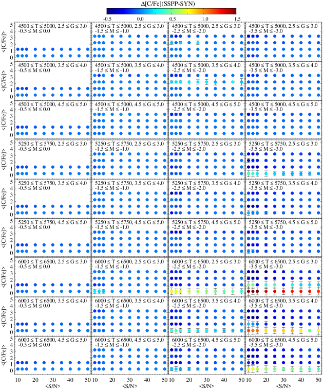
Figure 5.— Distributions of residuals in [C/Fe] between the SSPP and synthetic model values. $\langle$S/N$\rangle$ is an average signal-to-noise ratio per Angstrom, whereas $\langle$[C/Fe]$\rangle$ is an average value of the models with [C/Fe] = 0.0 to $+$0.5, $+$1.0 to $+$1.5, $+$2.0 to $+$2.5, and $+$3.0 to $+$3.5, that is, $\langle$[C/Fe]$\rangle$ = $+$0.25, $+$1.25, $+$2.25, and $+$3.25, respectively. The color-coded circles denote the difference in [C/Fe]; the scale of the differences is displayed as a color bar at the top. ‘SSPP’ denotes the SSPP values, while ‘SYN’ indicates the model values. The temperature (T), gravity (G), and metallicity (M) ranges are listed at the top of each panel.

From inspection of Figure 5 it is clear that, over most of the parameter regions, there are no large deviations in the zero point or scatter around the mean as a function of S/N for different carbon enhancements. However, as the metallicity decreases and temperature increases, the circle symbols turn from blue (indicating a small systematic offset in [C/Fe]) to yellow and red (indicative of a larger systematic offset in [C/Fe]), becoming quite severe for the lowest gravity and lowest [C/Fe] model spectra. The primary reason for this is that the CH $G$-band strength does not change much with varying carbon abundance in these low-metallicity, high-temperature, and especially C-normal ([C/Fe] $<+1.0$) regimes. This effect becomes worse for the low-gravity ranges ($\log~{}g$ $<3.0$); the strength of the CH $G$-band is almost indistinguishable among the models with different carbon abundances in the high-temperature, low-gravity, low-metallicity, and low-carbon abundance ranges. This causes a very broad and poorly constrained distribution of $\chi^{2}$ values as a function of [C/Fe], which results in unreliable estimate of [C/Fe] with much larger error ($>0.5$ dex). As a result, the low carbon-abundance models significantly deviate from the zero point in this parameter range, as seen in Figure 5. However, we do not expect to see many stars in the high-temperature ($T_{\rm eff}$ $>6000$ K), low-gravity ($\log~{}g$ $<3.0$) ranges in our SDSS/SEGUE sample (Presumably they would be red horizontal-branch stars, not main-sequence turnoff stars. See Section 4.1).

Except for this concern, it is clear that our technique reproduces [C/Fe] reasonably well, as the rms scatter between the SSPP analysis and the models are mostly less than 0.3 dex, without significant deviation in the zero points, over most of the parameter space down to S/N = 15 Å^-1.

3.3.2 Noise-added SDSS/SEGUE Spectra with High-resolution Parameters

We perform another noise-injection experiment for the spectra of stars listed in Table 1, following the same prescription described above. As we are not able to boost the S/N to values larger than the original S/N of a spectrum, we only generate the noise-added spectra up to a level below the original S/N of the SDSS/SEGUE spectrum. For example, the first entry (SDSS J142237.43+003105.2) in Table 1 has S/N = 44 Å^-1, and we create noise-injected spectra up to S/N = 40 Å^-1. Thus, for this spectrum, we generate spectra with S/N = 7.5, 10, 12.5, 15, 20, 25, 30, 35, and 40 Å^-1. As before, we produce 25 different realizations at each S/N value. The same procedure is applied to other stars. The star SDSS J220924.74$-$002859.8, with S/N = 15 Å^-1, only has noise-injected spectra up to S/N = 15 Å^-1.

Once generated, the noise-injected spectra are processed through the SSPP to obtain estimates of $T_{\rm eff}$, $\log~{}g$, [Fe/H], and [C/Fe], and we examine how each parameter changes with S/N. Table 3 summarizes the results of the experiment. The Gaussian mean ($\mu$) and sigma ($\sigma$) are calculated from considering all spectra that fall in each S/N bin (e.g., 39$\times$25 = 975 spectra for S/N = 10 Å^-1), after adjusting for the offsets of 52 K for $T_{\rm eff}$, –0.735 dex for $\log~{}g$, 0.177 dex for [Fe/H], and 0.128 dex for [C/Fe] (which are found in Figures 4 and 3, respectively).

Inspection of Table 3 indicates that the magnitude of the mean offsets and rms scatters generally increase with declining S/N for $T_{\rm eff}$, $\log~{}g$, [Fe/H], and [C/Fe]  as expected. Note that the rms scatters are calculated by following Equations (1) and (2). We assume errors of 0.3 dex in $\log~{}g$ and 0.15 dex in [Fe/H] for the high-resolution estimates, whereas we do not take into account the error in $T_{\rm eff}$ from the high-resolution results. One can notice from the table a very small offset in $T_{\rm eff}$, with scatter up to 170 K, relative to the high-resolution values, as the S/N decreases.

Table 3Impact of Signal-to-noise Ratios on Determination of $T_{\rm eff}$, $\log~{}g$, [Fe/H], and [C/Fe]

	$T_{\rm eff}$		$\log~{}g$		[Fe/H]		[C/Fe]
S/N	$\mu$	$\sigma$	$\mu$	$\sigma$	$\mu$	$\sigma$	$\mu$	$\sigma$
	(K)	(K)	(dex)	(dex)	(dex)	(dex)	(dex)	(dex)
10.0	$+$15	172	$+$0.086	0.680	$+$0.327	0.415	$-$0.162	0.485
12.5	$+$18	154	$+$0.078	0.614	$+$0.278	0.413	$-$0.137	0.465
15.0	$+$3	133	$+$0.102	0.400	$+$0.199	0.373	$-$0.107	0.353
20.0	$-$4	117	$+$0.033	0.335	$+$0.124	0.352	$-$0.074	0.355
25.0	$+$5	107	$+$0.022	0.345	$+$0.074	0.344	$-$0.023	0.332
30.0	$+$4	103	$+$0.005	0.297	$+$0.046	0.330	$-$0.012	0.310
35.0	$+$3	104	$-$0.004	0.259	$+$0.035	0.325	$-$0.004	0.324
40.0	$+$10	97	$+$0.000	0.213	$+$0.024	0.313	$+$0.002	0.309

Note. — The symbol $\mu$ is the Gaussian mean in the residuals between the SSPP and the high-resolution values, while $\sigma$ is calculated following Equations (1) and (2). These are derived after adjusting for offsets of 52 K for $T_{\rm eff}$, –0.735 dex for $\log~{}g$, 0.177 dex for [Fe/H], and 0.128 dex for [C/Fe], found in Figures 4 and 3, respectively.

As far as $\log~{}g$ and [Fe/H] are concerned, the offset generally increases, with larger scatter, as the quality of the spectrum decreases, again as expected. It is also seen that the mean offset in [C/Fe] becomes larger (in the sense of an underestimate of [C/Fe]) at low S/N. This presumably arises because, as a higher level of noise affects the region of the CH $G$-band, the feature becomes more washed out, resulting in a lower estimate of [C/Fe]. At S/N = 15 Å^-1, it appears that the size of the offsets for $\log~{}g$, [Fe/H], and [C/Fe] is less than 0.12 dex, which is smaller than the scatters listed in the table. The scatters for those three parameters are $\leq 0.4$ dex for S/N $\geq$ 15 Å^-1

One useful insight provided by this noise-injection experiment is that, at high S/N, the dominant error in the total uncertainty is the external error, $\langle\sigma_{\rm ext}\rangle$ in Equation (2), while at low S/N both the external and random error, $\sigma_{\rm SSPP}$ in Equation (2) contribute to the total error, as the size of the scatter become larger with declining S/N, as can be seen in Table 3.

We conclude from the noise-injection tests performed above that we are able to estimate [C/Fe] with a precision of $\sim$0.35 dex down to S/N = 15 Å^-1, while reproducing [Fe/H] estimates to better than 0.4 dex, with systematic offsets that are much smaller ($\sim 0.15$ dex). Previous experience suggests that noise experiments of the sort we have carried out are actually quite conservative in their predictions, so that the actual scatters in our estimates of [C/Fe] and [Fe/H] are likely to be smaller than indicated by these experiments.

There is one additional point that we need to address concerning the above results. We might expect that the error in the determination of [C/Fe] would vary with the metallicity of a star, such that the uncertainty of [C/Fe] will become larger in more metal-poor than metal-rich stars, especially for low carbon-abundance levels, as the CH $G$-band decreases in strength. Another small effect is the increase of atomic blending in the CH $G$-band region with increasing metallicity, which may also contribute to the uncertainty of [C/Fe]. Additional noise in the spectrum of a metal-poor star would drive the uncertainty to even higher values. As we validate our methods with a sample mostly comprising stars with [Fe/H] $<-2.5$, the associated errors of [Fe/H] and [C/Fe] might be larger in the stars with [Fe/H] $<-3.0$ than with [Fe/H] $>-3.0$ under the same S/N conditions.

In addition, owing to the scarcity of metal-rich stars in our comparison sample, we are not able to carry out a thorough test on the dependency of the uncertainty in the measured [C/Fe] with metallicity. However, we expect that the error associated with the [C/Fe] measurement for the stars with [Fe/H] $>-2.5$ will not be larger than the scatter (about 0.3 dex) found in Table 1, as the metal-rich stars possess much stronger CH $G$-band features.

4. The Carbon-Enhanced SDSS/SEGUE Stars

4.1. The SDSS/SEGUE Stellar Sample

All of the SDSS/SEGUE stellar spectra are processed through the latest version of the SSPP to obtain $T_{\rm eff}$, $\log~{}g$, [Fe/H], and [C/Fe]. In order to assemble a sample with reliable atmospheric parameters and [C/Fe] to analyze the nature of CEMP stars in the field, we first exclude all stars located on plug-plates that were taken in the direction of known open and globular clusters. For stars that were observed multiple times (these are often calibration or quality assurance stars), we retain only the spectrum with the highest S/N.

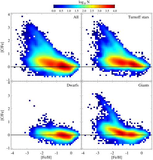
Figure 6.— Number–density distribution of the SDSS/SEGUE sample in the [C/Fe] and [Fe/H] plane, smoothed by a Gaussian kernel, for the entire sample (top-left panel), the turnoff stars (top-right panel), dwarfs (bottom-left panel), and giants (bottom-right panel). The turnoff stars are located in the temperature range 5600 K $\leq$ $T_{\rm eff}$ $\leq$ 6700 K. The dwarfs are occupy the ranges 4400 K $\leq$ $T_{\rm eff}$ $<$ 5600 K and $\log~{}g$ $\geq 4.0$, whereas the giant sample corresponds to the regions of 4400 K $\leq$ $T_{\rm eff}$ $<$ 5600 K and $\log~{}g$ $<4.0$. The solid horizontal lines are the solar value of [C/Fe]. The color bar at the top shows the number of stars per 0.1 $\times$ 0.1 dex bin.

Next, we remove all stars lacking information on their stellar parameters and [C/Fe], which can occur for a variety of reasons, but often because of defects in the spectra. We then apply the following (conservative) cuts to the sample: S/N $\geq 20$ Å^-1, 4400 K $\leq$ $T_{\rm eff}$ $\leq$ 6700 K, and –4.0 $\leq$ [Fe/H] $\leq+0.5$, so that our estimate of [C/Fe] is as reliable as possible. Finally, we visually inspect individual spectra with [Fe/H] $\leq-2.0$, to eliminate objects such as cool white dwarfs or stars with emission-line features in the cores of their Ca ii lines, which can produce spurious low-metallicity estimates from the SSPP. This visual inspection also removes a small number of additional defective spectra, which sometimes produces an incorrect metallicity estimate. In addition, we inspect the spectra for which the SSPP assigns [C/Fe] $\geq+0.7$ for [Fe/H] $>-2.0$, and remove stars with poor estimates of [Fe/H] and/or [C/Fe]. Furthermore, in our analysis of the CEMP stars below, we do not take into account the stars with unknown carbon status, which include those with the U (upper limit) flag raised and [C/Fe] $\geq+0.7$. There are about 1390 such stars. After application of these procedures, we end up with a total sample of about 247,350 stars.

We reiterate that, in our analysis of C-rich stars, we make use of the SSPP adopted metallicity, [Fe/H]_adopted and [C/Fe]_adjusted, computed from [C/H] – [Fe/H]_adopted, where [C/H] = [C/Fe] $+$ [Fe/H] through the carbon-determination routine; below we simply refer to our final abundance ratios as [C/Fe] and [Fe/H].

The top-left panel of Figure 6 is a logarithmic number-density map of the full sample of stars with accepted parameter estimates in the [C/Fe] versus [Fe/H] plane, after smoothing with a Gaussian kernel; each pixel is 0.1 dex by 0.1 dex. One notable feature seen in the panel is that, as the metallicity decreases, the distribution of [C/Fe] becomes gradually broader from [Fe/H] $<-0.5$ and [C/Fe] $\sim+0.7$, indicating that there exists a greater fraction of C-rich stars among the metal-poor stars. For this reason, we adopt the C-rich criterion of [C/Fe] $\geq+0.7$ in order for a star to be considered a CEMP star. Another interesting aspect of the panel is the dramatic increase seen in the number of stars with [C/Fe] $>+2.0$ below [Fe/H] $=-2.0$. That is, at a given metallicity below this value, the distribution of stars has a longer extended tail to high [C/Fe].

Additionally, the top-left panel shows a slightly increasing trend of [C/Fe] for the stars in the ranges [Fe/H] $<-1.5$ and [C/Fe] $<+1.0$. In order to investigate what kinds of objects contribute to this feature, and to be sure that it is not an artifact produced by incorrect [C/Fe] estimation, we divide our sample into main-sequence turnoff stars (top-right panel) with 5600 K $\leq$ $T_{\rm eff}$ $\leq$ 6700 K, dwarfs (bottom-left panel) with 4400 K $\leq$ $T_{\rm eff}$ $<$ 5600 K and $\log~{}g$ $\geq$ 4.0, and giants (bottom-right panel) with 4400 K $\leq$ $T_{\rm eff}$ $<$ 5600 K and $\log~{}g$ $<$ 4.0. It is clear that both the turnoff stars and giant stars contribute to the feature, and it is not produced by spurious measurement of [C/Fe] for some particular type of stars. However, compared to the dwarfs and giants, the turnoff stars with [Fe/H] $>-1.0$ and [C/Fe] $<+0.5$ tend to exhibit somewhat higher [C/Fe], by 0.2–0.3 dex. This level of the offset may be due not only to the uncertainty of the gravity estimate, owing to the relatively more difficult determination of $\log~{}g$ for such stars, but also to the generally weaker CH $G$-band features that are found for the warmer turnoff stars.

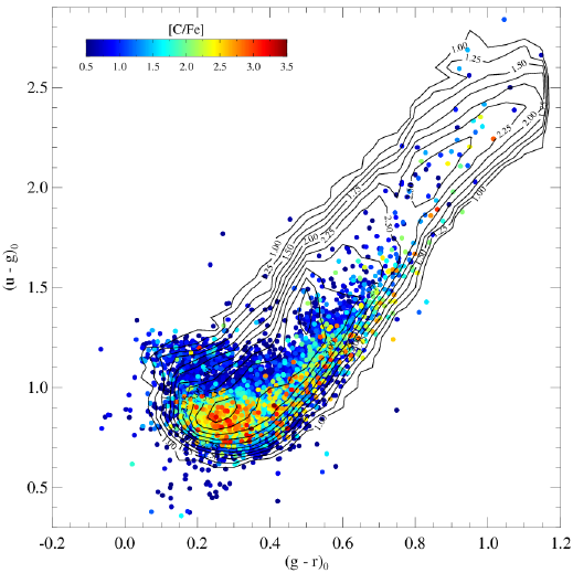
Figure 7.— Distribution of the stars in the reddening-corrected color–color plane $(u-g)_{0}$ and $(g-r)_{0}$ and with [C/Fe] $\geq+0.5$. The contours delineate the logarithmic number per 0.05 $\times$ 0.05 dex bin for the stars with [C/Fe] $<+0.5$. The color bar provides the scale for the carbon abundance ratios. Because most of the C-rich stars are metal-poor, the distribution is shifted toward the low side of the stellar locus. However, as all of the stars with different carbon enhancements occupy similar regions in the color–color plot, target selection in SDSS/SEGUE by color neither favors nor disfavors inclusion of the C-rich stars or the C-normal stars.

While the dwarf sample in the bottom-left panel of Figure 6 does not exhibit any unusual features, the bottom-right panel for the giants has a very intriguing branch of high-[C/Fe] stars below [Fe/H] $<-2.0$—a very well defined correlation between [C/Fe] and [Fe/H]. As Masseron et al. (2010) and Spite et al. (2013) pointed out, this might imply that, regardless of the metallicity range below [Fe/H] $<-2.0$, the stars in this branch may possess the same amount of carbon (similar [C/H]). In other words, there could exist a limit on the carbon abundances of material transferred from a progenitor AGB companion, due to the mass range of AGB stars that can produce and dredge up carbon-enriched material to their surfaces.

Another interesting property from the turnoff sample (top-right panel of Figure 6) is that it may be possible to separate the stars with [Fe/H] $<-2.5$ into three groups: C-normal with [C/Fe] $<+0.7$, C-intermediate with $+0.7<$ [C/Fe] $<+2.0$, and C-rich with [C/Fe] $>+2.0$. Interestingly enough, this feature does not arise for the dwarfs and giants. The intriguing features seen among the giants and turnoff stars requires further investigation, which is presently underway.

We have learned from the noise-added synthetic spectra that it is difficult to measure the carbon-to-iron ratio for hot, low-gravity stars with low carbon abundances, particularly for $T_{\rm eff}$ $>6000$ K and $\log~{}g$ $<3.0$. Our full sample of 247,350 objects includes only about 1600 stars with $T_{\rm eff}$ $>6000$ K and $\log~{}g$ $<3.0$, only about 0.6%. Thus, the impact on our analysis of the CEMP frequency is minimal.

Before using the SDSS/SEGUE stellar spectra to study the frequency of the CEMP phenomenon, it is necessary to ensure that the target selection by colors (e.g., $g-r$ and $u-g$) used in the SDSS/SEGUE does not bias toward or against the selection of carbon-rich stars, as the strong CH $G$-band may influence (primarily) the observed $g$ magnitude. To check on this possible selection bias, we construct a color-color plot in $(g-r)_{0}$ and $(u-g)_{0}$, shown in Figure 7. The contours delineate the logarithmic number for the stars with [C/Fe] $<+0.5$, while the filled circles represent the stars with [C/Fe] $\geq+0.5$. The carbon enhancement is color-coded, and its scale is shown at the top as a color bar. Since the C-rich stars are mostly occupied by metal-poor stars, the distribution is biased to the lower side of the stellar locus in the figure. From inspection of the figure, the stars with different carbon enhancements clearly occupy similar regions, without any isolated loci, in the color-color diagram, suggesting that the color selection of the targets in the SDSS/SEGUE does not preferentially select carbon-rich or carbon-normal stars.

4.2. The Frequency of CEMP Stars as a Function of [Fe/H]

4.2.1 Previous Studies

Spectroscopic follow-up of metal-poor candidates selected from the HK and HES surveys have identified a number of CEMP stars, and there have been numerous studies that attempted to derive their frequency, based on a number of different criteria. Different authors have employed minimum carbon-abundance ratios for CEMP stars of [C/Fe] $\geq+0.5$, $\geq+0.7$, or $\geq+1.0$. Aoki et al. (2007) and others have also included an additional luminosity criterion, in order to account for the reduction of [C/Fe] in advanced evolutionary stages along the red giant branch.

Based on a high-resolution spectroscopic analysis of 122 HES metal-poor giants, Cohen et al. (2005) claimed that the fraction of the CEMP stars ([C/Fe] $\geq+1.0$) is 14.4%$\pm$4% for [Fe/H] $\leq-2.0$. Frebel et al (2006) also derived a low CEMP fraction ([C/Fe] $\geq+1.0$), 9%$\pm$2%, from analysis of medium-resolution spectra for 145 VMP HES giants. They also found an increasing trend of CEMP frequency with distance above the Galactic plane. The claim was clearly confirmed by Carollo et al. (2012) from an analysis of a much larger sample of SDSS/SEGUE calibration stars.

On the other hand, based on high-resolution spectroscopy of 349 HES metal-poor stars from the HERES Survey (Christlieb et al. 2004; Barklem et al. 2005), Lucatello et al. (2006) calculated a lower limit of 21%$\pm$2% for CEMP stars ([C/Fe] $\geq+1.0$) for the stars with [Fe/H] $\leq-2.0$, higher than the previous two studies. This discrepancy may result from different sample selections, such as including a larger fraction of warm stars (making carbon features more difficult to detect) in the previous studies.

Similar to the present study, Carollo et al. (2012) determined [C/Fe] employing a $\chi^{2}$ minimization approach using spectral matching over the CH $G$-band region, and applied their technique to spectrophotometric and reddening standard stars from SDSS/SEGUE, resulting in about 31,200 stars with measured carbon-abundance ratios. Unlike our method, which allows two parameters to vary during the $\chi^{2}$ minimization step ([Fe/H] and [C/Fe]), they varied only [C/Fe]. Adopting the C-rich definition of [C/Fe] $\geq+0.7$, they obtained a cumulative frequency of 8% for [Fe/H] $\leq-1.5$, 12% for [Fe/H] $\leq-2.0$, and 20% for [Fe/H] $\leq-2.5$. They also showed that the enhancement of carbon relative to iron increases with declining metallicity, as the average [C/Fe] ($\langle$[C/Fe]$\rangle$ $\sim+1.0$) for CEMP stars at [Fe/H] = –1.5 grows to $\langle$[C/Fe]$\rangle$ $\sim+1.7$ at [Fe/H] = –2.7.

From an analysis of 25 giants in a sample of stars with [Fe/H] $\leq-2.5$ among 137 EMP ([Fe/H] $\leq-3.0$) candidates selected from SDSS/SEGUE, Aoki et al. (2013) derived a CEMP fraction (defined using [C/Fe] $\geq+0.7$) as high as 36%, substantially larger than any of the previous studies. However, they found only 10 CEMP stars out of 108 turnoff stars, yielding a fraction of 9%, which they argue is a lower limit due to the much weaker features of the CH $G$-band in these warmer stars.

Yong et al. (2013) have reported, for a large sample of halo stars with available high-resolution spectroscopy, that the C-rich population represents 32%$\pm$8% of stars below [Fe/H] = $-3.0$, (again using [C/Fe] $\geq+0.7$ as their CEMP criterion). These previous studies allow us to infer that the fraction of CEMP stars discovered to date roughly rises from 10% to 20% for [Fe/H] $<-2.0$ to 30% for [Fe/H] $<-3.0$, 40% for [Fe/H] $<-3.5$, and 75% for [Fe/H] $<-4.5$ (Beers & Christlieb 2005; Norris et al. 2007, 2013), after inclusion of a recently recognized star with [Fe/H] $\sim-5.0$ and [C/Fe] $\leq+0.7$ (which is not carbon enhanced, at least according to the [C/Fe] $\geq+1.0$ criterion; see Caffau et al. 2011).

4.2.2 Present Results

In order to investigate the previously noted trends with metallicity in more detail, we now derive the frequencies of CEMP stars based on the large sample of SDSS/SEGUE spectra. We note that, owing to the low resolution of the SDSS/SEGUE spectra, the accuracy of our determination of [C/Fe] is less than that based on high-resolution analysis. However, as our sample size is so much larger than previous studies, we expect to produce meaningful new results for the trends in CEMP frequency.

For clearly detected C-enhanced stars, we only count as C-rich objects those stars with [C/Fe] $\geq+0.7$, a correlation coefficient (CC) at least 0.7, and lacking an upper limit flag (‘U’). This sample of stars is regarded as $N_{\rm C}$. The CC is calculated by comparing the observed and synthetic spectrum over 4290–4318 Å. Then, the cumulative frequency of C-enhanced objects ($F_{\rm C}$) is computed by dividing the number of C-rich stars ($N_{\rm C}$) by all stars ($N_{\rm total}$), counted below a given metallicity ([Fe/H] = $+0.0,-0.5,-1.0,-1.5,-2.0,-2.5,-3.0,-3.5$). In the form of an equation,

$${F_{\rm C}}=\frac{N_{\rm C}([\rm C/\rm Fe]\geq+0.7,\rm CC\geq 0.7,D~{}or~{}L~{}flag)}{N_{\rm total}}.$$ (3)

Note that $N_{\rm total}$ in the denominator of the above expression includes all stars in the numerator, plus stars with [C/Fe] $\geq+0.7$ and CC $<0.7$, indicating a poor carbon measurement, the C-normal stars (D or L flag, [C/Fe] $<+0.7$), independent of the value of CC, and the stars with a U flag raised having [C/Fe] $<+0.7$, again independent of the value of CC. Stars with unknown carbon status, which include those with the U flag raised and [C/Fe] $\geq+0.7$, are not included in the above definition.

Table 4Cumulative Frequencies of CEMP Stars for Three Different Carbon Abundance Criteria

	SDSS/SEGUE $+$ Literature Sample							SDSS/SEGUE
	[C/Fe]$\geq+0.5$		[C/Fe]$\geq+0.7$		[C/Fe]$\geq+1.0$			[C/Fe]$\geq+0.5$		[C/Fe]$\geq+0.7$		[C/Fe]$\geq+1.0$
[Fe/H]	$N_{\rm C}$	$F_{\rm C}$	$N_{\rm C}$	$F_{\rm C}$	$N_{\rm C}$	$F_{\rm C}$	$N_{\rm total}$	$N_{\rm C}$	$F_{\rm C}$	$N_{\rm C}$	$F_{\rm C}$	$N_{\rm C}$	$F_{\rm C}$	$N_{\rm total}$
$\leq+0.0$	11622	0.05$\pm$0.01	5001	0.02$\pm$0.01	2641	0.01$\pm$0.01	243653	11581	0.05$\pm$0.01	4967	0.02$\pm$0.01	2612	0.01$\pm$0.01	243577
$\leq-0.5$	11548	0.06$\pm$0.01	4996	0.03$\pm$0.01	2640	0.01$\pm$0.01	191252	11507	0.06$\pm$0.01	4962	0.03$\pm$0.01	2611	0.01$\pm$0.01	191176
$\leq-1.0$	10792	0.11$\pm$0.01	4861	0.05$\pm$0.01	2627	0.03$\pm$0.01	96974	10751	0.11$\pm$0.01	4827	0.05$\pm$0.01	2598	0.03$\pm$0.01	96898
$\leq-1.5$	8386	0.16$\pm$0.01	3914	0.08$\pm$0.01	2222	0.04$\pm$0.01	51107	8345	0.16$\pm$0.01	3880	0.08$\pm$0.01	2193	0.04$\pm$0.01	51031
$\leq-2.0$	3799	0.25$\pm$0.01	2029	0.13$\pm$0.01	1171	0.08$\pm$0.01	15500	3758	0.24$\pm$0.01	1995	0.13$\pm$0.01	1142	0.07$\pm$0.01	15424
$\leq-2.5$	775	0.30$\pm$0.01	549	0.21$\pm$0.01	378	0.15$\pm$0.01	2587	734	0.29$\pm$0.01	515	0.21$\pm$0.01	349	0.14$\pm$0.01	2511
$\leq-3.0$	106	0.34$\pm$0.03	89	0.28$\pm$0.03	70	0.22$\pm$0.03	314	65	0.27$\pm$0.03	55	0.23$\pm$0.03	41	0.17$\pm$0.03	238
$\leq-3.5$	21	0.57$\pm$0.12	16	0.43$\pm$0.11	15	0.41$\pm$0.10	37	2	0.25$\pm$0.18	2	0.25$\pm$0.18	2	0.25$\pm$0.18	8

Note. — $N_{\rm C}$ is the number of stars within each metallicity range and with [C/Fe] $\geq$ $+$0.5, $+$0.7, or $+$1.0, and $F_{\rm C}$ is the fraction of the stars with [C/Fe] $\geq$ $+$0.5, $+$0.7, or $+$1.0, calculated from $N_{\rm C}/N_{\rm total}$, see text. The quoted error is derived from Poisson statistics. If the fraction of CEMP stars and its associated error is less than 1%, we assume to have at least 1%.

This approach to estimation of the frequency of CEMP stars is essentially the same as in Equation (2) of Carollo et al. (2012), except that they used the CH $G$-band strength ($>1.2$ Å) to indicate a clear detection of the CH $G$-band, rather than the CC criterion used in this study. As in Carollo et al. (2012), our calculated CEMP fraction is a lower limit, since some likely bona-fide CEMP stars with CC $<0.7$ are undercounted in the numerator of Equation (3) above, due to a poor spectrum (or with a poor match to the synthetic spectrum), and appear in the denominator instead.

Figure 8 shows the derived cumulative frequency of CEMP stars versus [Fe/H], with their associated Poisson error bars. The open squares indicate the calculation when considering only our SDSS/SEGUE stars, while the filled circles represent the fraction when including stars from the LS (mostly, Table 1 of Yong et al. 2013 and one object from Caffau et al. 2011), based on high-resolution analyses. Note that, in order to improve visibility, the $X$-axis ([Fe/H]) values of the open squares are shifted by $-0.02$ dex, while the filled circles are shifted by $+0.02$ dex.

The motivation for including the LS stars is to increase the number of stars with [Fe/H] $<-3.0$, for better number statistics in the derivation of the CEMP frequency in the lowest-metallicity regime. Before using the Yong et al. stars, we first remove the four SDSS/SEGUE stars in their sample. Some of the Yong et al. stars have two sets of [Fe/H] and [C/Fe] estimates reported; one from a dwarf analysis and the other from a subgiant analysis. We adopt the [Fe/H] and [C/Fe] values from the analysis under the assumption of dwarf luminosity classification for those stars to increase the number of dwarf stars. There are seven such stars, and they all have [C/Fe] $>+1.0$. No large differences in [C/Fe] and [Fe/H] exist between the dwarf and subgiant analyses.

Note also that, as the object from Caffau et al. (2011) in the LS is also one of the SDSS/SEGUE stars, we remove it from our SDSS/SEGUE sample to avoid double counting of this object. In Figure 8, the Poisson error bars are sufficiently large to be visible only for [Fe/H] $\leq-3.0$. Table 4 lists all derived quantities, including results obtained when adopting the CEMP criteria of [C/Fe] $\geq+0.5$ and $\geq+1.0$, for completeness. In the table, if the fraction of the CEMP stars or its associated error is less than 1%, we assume it to be 1%.

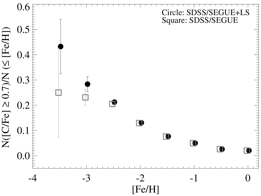
Figure 8.— Cumulative frequencies of CEMP stars ([C/Fe] $\geq+0.7$) in different metallicity ranges. [Fe/H] indicates the upper limit of the metallicity range considered at each plotted point. The open squares are the frequencies obtained by considering only the SDSS/SEGUE sample, while the filled circles include the literature sample (LS) from Yong et al. (2013) and Caffau et al. (2011). Poisson error bars are plotted. For clarity, the $X$-axis ([Fe/H]) values of the open squares are shifted by $-0.02$ dex, and the filled circles are shifted by $+0.02$ dex.

For [Fe/H] $<-3.0$, the sample including the LS stars exhibits a higher fraction of CEMP stars than the SDSS/SEGUE-only sample, although the error bars between the two samples overlap. This implies there are more C-rich stars ([C/Fe] $\geq+0.7$) for [Fe/H] $<-3.0$ in the LS than in the SDSS/SEGUE sample. Note also that, as listed in Table 4, there are only eight stars (two of which are CEMP stars) with [Fe/H] $\leq-3.5$ available, which precludes derivation of a statistically meaningful frequency for the SDSS/SEGUE sample at this metallicity.

When only considering the high-resolution sample from the literature, Yong et al. (2013) obtained a CEMP frequency of 32%$\pm$8% for stars with [Fe/H] $\leq-3.0$ and [C/Fe] $\geq+0.7$, which is larger by 9% than our derived value from the SDSS/SEGUE sample alone (23%$\pm$3%), but marginally compatible with theirs to within the error bars. When adopting [C/Fe] $\geq+1.0$ as the criterion for a CEMP star, Yong et al. (2013) estimated a frequency of 23%$\pm$6%, while our value is 17%$\pm$3%, which agrees well within the error bars.

Inspection of Figure 8 reveals that the cumulative CEMP frequency for the SDSS/SEGUE$+$LS sample (circle symbols in the figure) rises slowly from 2% at [Fe/H] $\leq 0.0$ to about 13% at [Fe/H] $\leq-2.0$ (close to that reported by Carollo et al. 2012), followed by a more rapid increase from [Fe/H] $\leq-2.0$ to [Fe/H] $\leq-3.5$. This trend does not differ when adopting other definitions for carbon enhancement ([C/Fe] $\geq+0.5$ or $\geq+1.0$), as seen in Table 4. It appears that our derived value of the CEMP frequency (8%$\pm$1% for [Fe/H] $\leq-2.0$ and [C/Fe] $\geq+1.0$) is closer to those of Cohen et al. (2005) and Frebel et al. (2006) than to that of Lucatello et al. (2006), but again, one must recall the possible selection effect in making this comparison. Our result for the cumulative frequency of CEMP stars ([C/Fe] $\geq+0.7$) with [Fe/H] $\leq-2.5$, 21%$\pm$1%, matches well with that obtained by Carollo et al. (20%).

Yong et al. (2013) examined the possibility that the CEMP fraction as a function of [Fe/H] continues to rise with declining metallicity below [Fe/H ] = –3.0. After dividing their objects with $-4.5\leq$ [Fe/H] $\leq-3.0$ into three bins with similar numbers of stars, they calculated the CEMP fractions in those three bins, and derived a slope of –0.24$\pm$0.22 for the CEMP frequencies for the stars with [Fe/H] $\leq-3.0$, which included three stars with [Fe/H] $<-4.5$. The inclusion of the star (with [Fe/H] $\sim-5.0$ with [C/Fe] $\leq+0.7$) from Caffau et al. (2011) yields a slope of –0.20$\pm$0.19. Based on these results, they concluded that there was no significant correlation between the fraction of CEMP stars and [Fe/H] among stars of the lowest metallicity.

Figure 9 shows the differential frequencies of CEMP stars in each bin of [Fe/H] from the SDSS/SEGUE$+$LS sample. Table 5 lists the metallicity bins used, average metallicity in each bin, and the fraction of the CEMP stars in each metallicity bin. The observed trend of the differential CEMP frequency from the figure is that it steadily increases from 1% at [Fe/H] $\sim-1.0$ to 75% at [Fe/H] $\sim-5.25$.

Figure 9.— Differential frequencies of CEMP stars ([C/Fe] $\geq+0.7$) as a function of [Fe/H]. The bin with [Fe/H] $<-5.0$ has only four stars, as listed in Table 5, one of which is from Caffau et al. (2011), and assumed to be a C-normal star. The red-solid line is the slope obtained by fitting the frequencies for [Fe/H] $\leq-3.0$, while the blue-solid line is the slope derived from the sub-sample in the range [Fe/H] $<-2.0$. Poisson error bars are plotted. The dashed lines indicate the 1$\sigma$ errors in the derived slopes after taking into account the measured Poisson error in the calculated frequencies.

Calculating the slopes of the CEMP fractions from these observations, we obtain a slope of –0.23$\pm 0.13$ from a linear fit to the fractions with [Fe/H] $\leq-3.0$, shown as a red-solid line in the figure. The dashed lines are 1$\sigma$ errors in the computed slope (note that the measured Poisson error in the fraction of each metallicity bin is taken into account during the fit). This value is in good agreement from that of Yong et al. (–0.20, after the inclusion of Caffau et al.’s star). Extending the metallicity range up to [Fe/H] = –2.0, the derived slope is –0.17$\pm 0.01$, shown as a blue-solid line in the figure, which is not far from that of the more metal-poor region, and certainly is consistent to within the allowed errors. Thus, this overall behavior suggests there exists at most a mildly increasing differential frequency of CEMP stars with decreasing metallicity. However, because there are not many stars below [Fe/H] = –3.5 discovered to date, more objects are required to obtain confident estimates of the CEMP frequency at the lowest metallicities.

Table 5Differential Frequencies of CEMP Stars in Bins of Metallicity from the SDSS/SEGUE and Literature Samples

[Fe/H] Range	$\langle$[Fe/H]$\rangle$	$N_{\rm C}$	$N_{\rm total}$	$F_{\rm C}$
$-1.25\leq[\rm Fe/H]<-1.00$	$-1.12$	262	20876	0.01$\pm$0.01
$-1.50\leq[\rm Fe/H]<-1.25$	$-1.38$	685	24991	0.03$\pm$0.01
$-1.75\leq[\rm Fe/H]<-1.50$	$-1.62$	907	21359	0.04$\pm$0.01
$-2.00\leq[\rm Fe/H]<-1.75$	$-1.87$	978	14248	0.07$\pm$0.01
$-2.25\leq[\rm Fe/H]<-2.00$	$-2.11$	873	8584	0.10$\pm$0.01
$-2.50\leq[\rm Fe/H]<-2.25$	$-2.36$	607	4329	0.14$\pm$0.01
$-2.75\leq[\rm Fe/H]<-2.50$	$-2.61$	339	1708	0.20$\pm$0.01
$-3.00\leq[\rm Fe/H]<-2.75$	$-2.85$	122	567	0.22$\pm$0.02
$-3.25\leq[\rm Fe/H]<-3.00$	$-3.10$	51	206	0.25$\pm$0.03
$-3.50\leq[\rm Fe/H]<-3.25$	$-3.36$	22	73	0.30$\pm$0.06
$-4.50\leq[\rm Fe/H]<-3.50$	$-3.74$	13	33	0.39$\pm$0.11
$-6.00\leq[\rm Fe/H]<-4.50$	$-5.28$	3	4	0.75$\pm$0.43

Note. — $\langle$[Fe/H]$\rangle$ is an average of [Fe/H] in each metallicity range. $N_{\rm C}$ is the number of C-rich stars ([C/Fe] $\geq 0.7$) within each metallicity range, and $F_{\rm C}$ is the frequency of the CEMP stars calculated by $N_{\rm C}/N_{\rm total}$, see text. The quoted error is derived from Poisson statistics. If the fraction of the CEMP stars and its associated error is less than 1%, we assume it to be at least 1%.

Nonetheless, Figure 9 provides us with an overall accurate trend of steadily increasing CEMP fractions with decreasing metallicity, confirming and extending the results of previous studies, with much improved Poisson errors compared to past efforts. Another important point evident from inspection of the figure is that the differential frequency of CEMP stars may change somewhat rapidly from one metallicity bin to another, especially for [Fe/H] $<-2.0$, hence as “fine-grained” a sample as possible is required to be sensitive to this behavior, which may contain clues to the nature of the progenitor stellar populations of CEMP stars.

4.3. Frequencies of CEMP Stars among Giants, Turnoff Stars, and Dwarfs

Aoki et al. (2013) derived a CEMP frequency (defined using [C/Fe] $\geq+0.7$) as high as 36% for their giant stars, but a frequency of only 9% was obtained for their main-sequence turnoff stars (which they considered a lower limit). One caution to be aware of in their analysis is that there might be a bias in their high-resolution spectroscopic sample, since they made use of the CH $G$-band to select CEMP candidates, although it is much weaker for the warmer turnoff stars. Thus, their frequency estimate for stars near the turnoff will only include stars with higher carbon abundance ratios (e.g., [C/Fe] $\sim+1.5$ for [Fe/H] $\sim-3.0$; see Aoki et al. 2013).

On the other hand, Yong et al. (2013) also obtained a higher CEMP fraction for dwarfs in their sample (50%$\pm$31%) than for giants (39%$\pm$11%), although these estimates overlap within the errors. These results suggest the possibility that the fraction of the CEMP stars varies between different luminosity classes.

We now examine how the cumulative frequency of CEMP stars differs among giants, turnoff stars, and dwarfs in our SDSS/SEGUE+LS sample. The classifications used for each category are—giant: 1.0 $<$ $\log~{}g$ $\leq$ 3.5, turnoff: 3.5 $<$ $\log~{}g$ $\leq$ 4.2, and dwarf: 4.2 $<$ $\log~{}g$ $\leq$ 5.0. We stress again that we adopt the parameters from the dwarf analysis in the LS from Yong et al. (2013) in order to increase the size of the dwarf sample. Had we taken the assumed gravity for the subgiant analysis, six additional stars would have been included in the turnoff sub-sample, while one object would belong to the giant sub-sample, instead of all being dwarfs in our luminosity classifications; the CEMP frequencies would change accordingly.

Because the turnoff and giant stars probe more distant regions of the Galaxy than the dwarfs, the possibility exists that the change of the CEMP frequency may be influenced by changes in the mix of populations (inner halo versus outer halo). Thus, we also investigate the CEMP fraction for stars located within 5 kpc of the Galactic mid-plane (i.e., $|Z|<5$ kpc). This distance condition rejects some of the giant and turnoff stars, but includes most of the dwarfs.

Figure 10 shows the changes in the cumulative fractions of CEMP stars with [Fe/H]. The circles represent giants, the squares the turnoff stars, and the triangles the dwarfs. The open symbols denote the sample with $|Z|<5$ kpc. The star symbols indicate the CEMP frequencies, without the luminosity classifications, within $|Z|$ = 5 kpc. We follow Equation 3 to compute the fraction for each population. The computed fraction for each sub-sample over various metallicity ranges is listed in Table 6 for the entire sample, and for the sub-sample restricted by the vertical distance criterion. Note that, for clarity, the $X$-axis ([Fe/H]) values of the open triangles and circles are shifted by $+0.05$ dex, whereas the open squares are shifted by $-0.05$ dex.

Examining first the filled symbols in Figure 10, which are derived without application of the distance cut, the general trend of the cumulative frequency of the CEMP giants is quite intriguing. Unlike the steady increase of the CEMP frequency for the turnoff stars and dwarfs, the CEMP fraction of the giants does not increase, but remains almost at the same value below [Fe/H] = – 2.5. This may be due to the expected dilution of carbon by CNO-processed material from the interiors of these stars, as is argued to have occurred for other samples of metal-poor giants by Spite et al. (2006).

The cumulative frequency of CEMP giants for [Fe/H] $\leq-2.5$ (32%$\pm$2%) is in good agreement with that of Aoki et al. (2013) (36%$\pm$12%), while the fraction for [Fe/H] $\leq\ -3.0$ (31%$\pm$4%) is slightly lower than that of Yong et al. (2013) for their giant sample (39%$\pm$11%). However, all of these measurements are close enough to be consistent within the claimed Poisson errors. The cumulative CEMP frequency (12%$\pm$1%) of our giant sample in the range of [Fe/H] $\leq-2.0$ (and using [C/Fe] $\geq+1.0$) is closer to that reported by Cohen et al. (2005), 14%$\pm$4%, than that by Frebel et al. (2006), 9%$\pm$2%.

Figure 10.— Cumulative frequencies of CEMP stars ([C/Fe] $\geq+0.7$) from the SDSS/SEGUE$+$LS sample, as a function of [Fe/H], for three different luminosity classes: giants (circles), main-sequence turnoff stars (squares), and dwarfs (triangles). We assume classifications based on the measured surface gravity—giant: $1.0\leq$ $\log~{}g$ $<3.5$, turnoff: $3.5\leq$ $\log~{}g$ $<4.2$, and dwarf: $4.2\leq$ $\log~{}g$ $<5.0$. Poisson error bars are plotted. For an alternative comparison, we also restrict the sample to stars within 5 kpc from the Galactic mid-plane; the open symbols represent the frequencies from the distance-restricted sample. The star symbols are the frequency of CEMP stars from all stars with $|Z|<5$ kpc. The blue-solid line shows the frequencies calculated in Figure 8, without any restriction on distance from the plane. For clarity, the $X$-axis ([Fe/H]) values of the open triangles and circles are shifted by $+0.05$ dex, while the open squares are shifted by $-0.05$ dex.

For the main-sequence turnoff stars, the figure indicates that the CEMP frequency initially slowly increases with decreasing metallicity, but exhibits a rapid increase below [Fe/H] = –2.5. We obtain a frequency of 10%$\pm$1% for [Fe/H] $\leq-2.5$, which is in good agreement with that reported by Aoki at al. (2013), 9%$\pm$3%.

The observed change in the cumulative frequency of CEMP stars for the dwarfs is rather dramatic. The dwarf population exhibits a very rapid increase in the fraction of the CEMP stars below [Fe/H] = –2.5, jumping from about 15%$\pm$4% at [Fe/H] $\leq-2.5$ to 75%$\pm$22% at [Fe/H] $\leq-3.0$. Our sample suggests that all dwarfs are CEMP stars below [Fe/H] = –3.5, but this is based on a sample of only four stars. In fact, these all come from the previous studies compiled by Yong et al. (2013). A larger sample of dwarfs in this metallicity range will be needed in order to confirm this behavior.

We now consider the effect that application of a distance restriction ($|Z|<5$ kpc) to the sample has on the derived CEMP frequencies. For giant and turnoff stars, the CEMP fraction changes rather significantly for [Fe/H] $\leq-2.5$. Inspection of Figure 10 reveals that the frequency of the CEMP giants within 5 kpc of the Galactic mid-plane (open circles) does not appear to increase below [Fe/H] = –2.5, but rather, levels off to a roughly constant value. By comparison, the CEMP frequencies of the turnoff sample within $|Z|<5$ kpc (open squares) becomes even higher than that of the entire turnoff sample (filled squares) below [Fe/H] = $-3.0$. This may suggest that the mix of a greater fraction of EMP ([Fe/H] $<-3.0$) turnoff stars relative to giants present among the stars with $|Z|<5$ kpc would result in an overall higher frequency of CEMP stars. This effect can be confirmed from the observed cumulative CEMP fractions, computed from all stars within $|Z|=5$ kpc.

Table 6Cumulative Frequencies of CEMP Stars Classified as Giants, Turnoff Stars, and Dwarfs from the SDSS/SEGUE and Literature Samples

	All									$|Z|<5$ kpc
	Giant			Turnoff			Dwarf			Giant			Turnoff			Dwarf
[Fe/H]	$N_{\rm C}$	$N_{\rm total}$	$F_{\rm C}$	$N_{\rm C}$	$N_{\rm total}$	$F_{\rm C}$	$N_{\rm C}$	$N_{\rm total}$	$F_{\rm C}$	$N_{\rm C}$	$N_{\rm total}$	$F_{\rm C}$	$N_{\rm C}$	$N_{\rm total}$	$F_{\rm C}$	$N_{\rm C}$	$N_{\rm total}$	$F_{\rm C}$
$\leq+0.0$	2206	32995	0.07$\pm$0.01	2629	80898	0.03$\pm$0.01	159	129648	0.01$\pm$0.01	793	14802	0.05$\pm$0.01	2242	74910	0.03$\pm$0.01	156	128959	0.01$\pm$0.01
$\leq-0.5$	2205	32042	0.07$\pm$0.01	2627	69327	0.04$\pm$0.01	157	89772	0.01$\pm$0.01	792	13916	0.06$\pm$0.01	2240	63515	0.04$\pm$0.01	154	89216	0.01$\pm$0.01
$\leq-1.0$	2174	27817	0.08$\pm$0.01	2530	42905	0.06$\pm$0.01	150	26141	0.01$\pm$0.01	763	10543	0.07$\pm$0.01	2150	37750	0.06$\pm$0.01	147	25879	0.01$\pm$0.01
$\leq-1.5$	1916	17652	0.11$\pm$0.01	1886	24244	0.08$\pm$0.01	105	9111	0.01$\pm$0.01	554	5827	0.10$\pm$0.01	1586	21044	0.08$\pm$0.01	102	9031	0.01$\pm$0.01
$\leq-2.0$	1179	6138	0.19$\pm$0.01	804	7804	0.10$\pm$0.01	39	1484	0.03$\pm$0.01	239	1357	0.18$\pm$0.01	656	6414	0.10$\pm$0.01	38	1476	0.03$\pm$0.01
$\leq-2.5$	420	1330	0.32$\pm$0.02	110	1117	0.10$\pm$0.01	16	108	0.15$\pm$0.04	62	229	0.27$\pm$0.03	90	808	0.11$\pm$0.01	15	106	0.14$\pm$0.04
$\leq-3.0$	59	192	0.31$\pm$0.04	17	101	0.17$\pm$0.04	12	16	0.75$\pm$0.22	11	51	0.22$\pm$0.07	16	66	0.24$\pm$0.06	12	16	0.75$\pm$0.22
$\leq-3.5$	9	27	0.33$\pm$0.11	3	6	0.50$\pm$0.29	4	4	1.00$\pm$0.50	3	14	0.21$\pm$0.12	3	4	0.75$\pm$0.43	4	4	1.00$\pm$0.50

Note. — Two samples of stars are considered. One includes all stars, while the other one consists of stars within $\pm 5$ kpc from the Galactic plane (e.g., $|Z|<5$ kpc). $N_{\rm C}$ is the number of CEMP stars ([C/Fe] $\geq 0.7$) within each metallicity range, and $F_{\rm C}$ is the fraction of the CEMP stars calculated by $N_{\rm C}/N_{\rm total}$, see text. The quoted error is derived from Poisson statistics. If the fraction of the CEMP stars and its associated error is less than 1%, we assume it to be at least 1%. We consider the stars in the surface-gravity range 1.0 $\leq$ $\log~{}g$ $<$ 3.5, 3.5 $\leq$ $\log~{}g$ $<$ 4.2, and 4.2 $\leq$ $\log~{}g$ $<$ 5.0, to be a giants, turnoff stars, and dwarfs, respectively.

Another interesting point to be drawn from Figure 10 is that, in the metallicity regime $-2.5\leq$ [Fe/H] $\leq-1.5$, the CEMP frequency derived from all stars with $|Z|<5$ kpc is slightly lower than the CEMP fraction without application of a distance restriction (blue-solid line; the same sample shown in Figure 8). This behavior is consistent with previous demonstrations that the CEMP frequency increases with increasing distance from the Galactic plane, indicating that there may exist a greater fraction of CEMP stars associated with the outer-halo population than the inner-halo population (Carollo et al. 2012).

Figure 10 also implies that, as the giants are intrinsically brighter than the turnoff and dwarf stars (hence are more likely to be observed beyond $|Z|=5$ kpc), one might expect a bias toward lower derived frequencies of CEMP stars if the sample under consideration extends to include larger volumes of the Galaxy. We conclude that a volume-limited sample that populates different stellar luminosity classes as equally as possible should be used to obtain more meaningful comparisons of their respective CEMP frequencies as a function of [Fe/H] or $|Z|$. A more detailed analysis and interpretation of the dependence of the frequency of CEMP stars on their kinematic properties and spatial distribution will be presented in a future paper.

5. Summary and Conclusions

We have presented a method for estimating [C/Fe] from the low-resolution ($R=2000$) SDSS/SEGUE stellar spectra, based on spectral matching against a custom grid of synthetic spectra. In order to validate our method, we have performed a star-by-star comparison between the SDSS/SEGUE spectra of stars with available high-resolution determinations of [C/Fe], carried out tests of the impact of $T_{\rm eff}$ and $\log~{}g$ errors on the determination of [Fe/H] and [C/Fe], and conducted noise-injection experiments on both the synthetic spectra and SDSS/SEGUE stars with literature values of [C/Fe] based on high-resolution spectroscopy,

Checks on possible errors in our determination of [C/Fe] due to our preference of fixing $T_{\rm eff}$ and $\log~{}g$ at the values delivered by the SSPP reveals that the mean offsets associated with different input shifts in $T_{\rm eff}$ and $\log~{}g$ are mostly smaller than the derived rms scatter in the determination of [C/Fe]. We confirm that the surface-gravity error in the SSPP has only a minor impact on our measured [C/Fe]. Within $T_{\rm eff}$ shifts of $\pm$200 K (which is equivalent to the typical error of the SSPP-determined $T_{\rm eff}$), our determined [C/Fe] is perturbed by less than $\pm$0.25 dex, which is smaller than the rms scatter of 0.30 dex, the typical error of our measured [C/Fe].

Our noise-injection experiments suggests that our approach is capable of estimating [C/Fe] with a precision $<$ 0.35 dex for spectra with S/N $\geq 15$ Å^-1 over the parameter space $T_{\rm eff}$ = [4400, 6700] K, $\log~{}g$ = [1.0, 5.0], [Fe/H] = [–4.0, $+$0.0], and [C/Fe] = [$-$0.25, $+3.5$]. According to our noise-injection experiments, errors in the determination of [C/Fe] increase to $\sim$0.35 dex for S/N $<15$ Å^-1. Thus, it is recommended to use the spectra with a minimum S/N = 15 Å^-1 for the application of this approach.

The method presented here can be easily applied to other spectra that cover similar wavelength ranges at similar resolving power. Therefore, it should be a useful new tool for the investigation of the chemical-enrichment history of Galactic populations, with stellar spectra obtained by other large spectroscopic surveys such as LAMOST.

Using the SDSS/SEGUE and LS, we have investigated how the differential frequency of CEMP stars changes as a function of [Fe/H]. We find that the CEMP frequency slowly rises from almost zero (1%) to about 14%$\pm$1% at [Fe/H] $\sim$ –2.4, and there is a marked increase, by about a factor of three (39%), from [Fe/H] $\sim$ –2.4 to $\sim$ –3.7. The gradient of the CEMP fraction does not change much over different metallicity regimes, suggesting a steady increase of the frequency of CEMP stars with decreasing metallicity. However, owing to the handful of stars with [Fe/H] $<$–3.5 identified to date, it is necessary to collect more stars in this range to robustly characterize the CEMP frequency for extremely and ultra-metal poor stars.

We have also investigated how the cumulative frequency of CEMP stars varies between different luminosity classes. Unlike the dwarfs and turnoff stars, which show continuously rising trends below [Fe/H] = –2.5, the giant sample exhibits a roughly constant CEMP fraction below [Fe/H] $\leq-2.5$. The giant sample exhibits a fraction of CEMP stars for [Fe/H] $\leq-2.5$ of 32%, which is in good agreement with that reported by Aoki et al. (2013) (36%), while the fraction of CEMP giant stars for [Fe/H] $\leq-3.0$ (31%) is somewhat lower than that of Yong et al. (2013) (39%). In both cases the Poisson error bars overlap. For the main-sequence turnoff stars we obtain a CEMP fraction of 10% for [Fe/H] $\leq-2.5$, in excellent agreement with that of Aoki at al. (2013) (9%). However, as Aoki et al. (2013) illustrated, there remains the difficulty of identifying CEMP stars in this temperature regime due to the low resolution of the SDSS/SEGUE spectra, such that the CH $G$-band can only be detected for stars with higher carbon abundances. Lastly, the dwarf stars exhibit a very rapid increase in the cumulative frequency of CEMP stars below [Fe/H] = –2.5, leaping from a fraction of 15% at [Fe/H] $\leq-2.5$ to about 75% at [Fe/H] $\leq$ –3.0. All of the dwarfs with [Fe/H] $\leq-3.5$ come from previous high-resolution studies, and all are CEMP stars. Since it is only based on a sample of four stars, the sample size must be substantially increased in order to confirm this result.

Analysis of a distance-restricted sample ($|Z|<5$ kpc) reveals that the cumulative frequency of CEMP stars classified as giants does not appear to increase with declining metallicity, but rather, remains roughly constant below [Fe/H] = –2.5. On the other hand, the cumulative frequencies of the turnoff sample of CEMP stars increases below [Fe/H] = –3.0, indicating that a sample biased to include more EMP turnoff stars than giants (as might arise from examination of a local volume), may result in an overall trend of higher CEMP frequencies with decreasing metallicity. As discussed by Lucatello et al. (2006), Spite et al. (2006), and Aoki et al. (2007), the apparent lack of an increase in the frequency of CEMP stars among giants could well be associated with extra mixing of CNO-processed material from their interiors, diluting the C-rich material in their envelopes. Confirmation of this effect could come from observations of the ¹²C/¹³C and [N/Fe] ratios for such stars. Inspection of the distance-restricted sample also indirectly confirms the increasing trend of CEMP frequency with increasing distance from the Galactic mid-plane, previously pointed out by Frebel et al. (2006) and Carollo et al. (2012). Future analysis of this sample, taking into account a more detailed examination of the kinematics and spatial distribution of these stars, should prove illuminating.

References

- (1) Abate, C., Pols, O. R., Izzard, R. G., Mohamed, S. S., & de Mink, S. E. 2013, A&A, 552, 26
- (2) Abazajian, K., Adelman-McCarthy, J. K., Agüeros, M. A., et al. 2003, AJ, 126, 2081
- (3) Abazajian, K., Adelman-McCarthy, J. K., Agüeros, M. A., et al. 2004, AJ, 128, 502
- (4) Abazajian, K., Adelman-McCarthy, J. K., Agüeros, M. A., et al. 2005, AJ, 129, 1755
- (5) Abazajian, K., Adelman-McCarthy, J. K., Agüeros, M. A., et al. 2009, ApJS, 182, 543
- (6) Abia, C., Busso, M., Gallino, R., et al. 2001, ApJ, 559, 1117
- (7) Adelman-McCarthy, J. K., Agüeros, M. A., Allam, S. S., et al. 2006, ApJS, 162, 38
- (8) Adelman-McCarthy, J. K., Agüeros, M. A., Allam, S. S., et al. 2007, ApJS, 172, 634
- (9) Adelman-McCarthy, J. K., Agüeros, M. A., Allam, S. S., et al. 2008, ApJS, 175, 297
- (10) Ahn, C. P., Alexandroff, R., Allende Prieto, C., et al. 2012, ApJS, 203, 21
- (11) Aihara, H., Allende Prieto, C., An, D., et al. 2011, ApJS, 193, 29
- (12) Allende Prieto, C., Beers, T. C., Wilhelm, R., et al. 2006, ApJ, 636, 804
- (13) Allende Prieto, C., Sivarani, T., Beers, T. C., et al. 2008, AJ, 136, 2070
- (14) Alvares, R., & Plez, B. 1998, A&A, 330, 1109
- (15) Aoki, W., Beers, T. C., Christlieb, N., et al. 2007, ApJ, 655, 492
- (16) Aoki, W., Beers, T. C., Lee, Y. S., et al. 2013, AJ, 145, 13
- (17) Aoki, W., Beers, T. C., Sivarani, T., et al. 2008, ApJ, 678, 1351
- (18) Asplund, M., Grevesse, N., & Sauval, A. J. 2005, in ASP Conf. Ser. 336, Cosmic Abundances as Records of Stellar Evolution and Nucleosynthesis, ed. T. G. Barnes III & F. N. Bash (San Francisco, CA: ASP), 25
- (19) Bailer-Jones, C. A. L. 2000, A&A, 357, 197
- (20) Barklem, P. S., Christlieb, N., Beers, T. C., et al. 2005, A&A, 439, 129
- (21) Barklem, P. S., O’Mara, B. J. 1998, MNRAS, 300, 863
- (22) Beers, T. C., Carollo, D., Ivezić, Ž., et al. 2012, ApJ, 746, 34
- (23) Beers, T. C., Chiba, M., Yoshii, Y., et al. 2000, AJ, 119, 2866
- (24) Beers, T. C., & Christlieb, N. 2005, ARA&A, 43, 531
- (25) Beers, T. C., Preston, G. W., & Shectman, S. A. 1985, AJ, 90, 2089
- (26) Beers, T. C., Preston, G. W., & Shectman, S. A. 1992, AJ, 103, 1987
- (27) Beers, T. C., Rossi, S., Norris, J. E., Ryan, S. G., & Shefler, T. 1999, AJ, 117, 981
- (28) Bisterzo, S., Gallino, R., Straniero, O., Cristallo, S., & Käppeler, F. 2011, MNRAS, 418, 284
- (29) Bisterzo, S., Gallino, R., Straniero, O., Cristallo, S., & Käppeler, F. 2012, MNRAS, 422, 849
- (30) Bond, H. E. 1974, ApJ, 194, 95
- (31) Caffau, E., Bonifacio, P., François, P., et al. 2011, Natur, 477, 67
- (32) Carollo, D., Beers, T. C., Bovy, J., et al. 2012, ApJ, 744, 195
- (33) Cayrel, R., Depagne, E., Spite, M., et al. 2004, A&A, 416, 1117
- (34) Christlieb, N. 2003, RvMA, 16, 191
- (35) Christlieb, N., Beers, T. C., Barklem, P. S., et al. 2004, A&A, 428, 1027
- (36) Christlieb, N., Green, P. J., Wisotzki, L., & Reimers, D. 2001, A&A, 375, 66
- (37) Christlieb, N., Schörck, T., Frebel, A., et al. 2008, A&A, 484, 721
- (38) Cohen, J. G., Christlieb, N., McWilliam, A., et al. 2008, ApJ, 672, 320
- (39) Cohen, J. G., Shectman, S., Thompson, I., et al. 2005, ApJ, 633, L109
- (40) Cooke, R., Pettini, M., Steidel, C. C., Rudie, G. C., & Nissen, P. E. 2011, MNRAS, 417, 1534
- (41) Cui, X.-Q., Zhao, Y.-H., Chu, Y.-Q., et al. 2012, RAA, 12, 1197
- (42) Dekker, H., D’Odorico, S., Kaufer, A., Delabre, B., & Kotzlowski, H. 2000, Proc. SPIE, 4008, 534
- (43) Frebel, A., Christlieb, N., Norris, J. E., et al. 2006, ApJ, 652, 1585
- (44) Frebel, A., & Norris, J. 2013, Planets, Stars and Stellar Systems, Vol. 5, ed. T. D. Oswalt & G. Gilmore (Dordrecht: Springer). 55
- (45) Fukugita, M., Ichikawa, T., Gunn, J. E., et al. 1996, AJ, 111, 1748
- (46) Gunn, J. E., Carr, M., Rockosi, C., et al. 1998, AJ, 116, 3040
- (47) Gunn, J. E., Siegmund, W. A., Mannery, E. J., et al. 2006, AJ, 131, 2332
- (48) Gustafsson, B., Edvardsson, B., Eriksson, K., et al. 2008, A&A, 486, 951
- (49) Herwig, F. 2005, ARA&A, 43, 435
- (50) Hill, V., Plez, B., Cayrel, R., et al. 2002, A&A, 387, 560
- (51) Ito, H., Aoki, W., Beers, T. C., et al. 2013, ApJ, 773, 33
- (52) Ito, H., Aoki, W., Honda, S., & Beers, T. C. 2009, ApJ, 698, L37
- (53) Izzard, R. G., Glebbeek, E., Stancliffe, R. J., & Pols, O. R. 2009, A&A, 508, 1359
- (54) Johnson, J. A. 2002, ApJS, 139, 219
- (55) Keenan, P. C. 1942, ApJ, 96, 101
- (56) Kupka, F., Piskunov, N., Ryabchikova, T. A., Stemples, H. C., Weiss, W. W. 1999, AAS, 138, 119
- (57) Lai, D. K., Bolte, M., Johnson, J. A., et al. 2008, ApJ, 681, 1524
- (58) Lee, Y. S., Beers, T. C., Allende Prieto, C., et al. 2011, AJ, 141, 90
- (59) Lee, Y. S., Beers, T. C., Sivarani, T., et al. 2008a, AJ, 136, 2022
- (60) Lee, Y. S., Beers, T. C., Sivarani, T., et al. 2008b, AJ, 136, 2050
- (61) Lucatello, S., Beers, T. C., Christlieb, N. C., et al. 2006, ApJ, 652, L37
- (62) Lucatello, S., Gratton, R. G., Beers, T. C., & Carretta, E. 2005, ApJ, 625, 833
- (63) Luo, A.-L., Zhang, H.-T., Zhao, Y.-H., et al. 2012, RAA, 12, 1243
- (64) Markwardt, C. B. 2009, in ASP Conf. Ser. 411, Astronomical Data Analysis Software and Systems XVIII, ed. D. A. Bohlender, D. Durand, & P. Dowler (San Francisco, CA: ASP), 251
- (65) Marsteller, B., Beers, T. C., Rossi, S., et al. 2005, NuPhA, 758, 312
- (66) Masseron, T. 2006, PhD thesis, Observatoire de Paris, France
- (67) Masseron, T., Johnson, J. A., Plez, B., et al. 2010, A&A, 509, 93
- (68) Matsuoka, K., Nagao, T., Maiolino, R., Marconi, A., & Taniguchi, Y. 2011, A&A, 532, L10
- (69) McWilliam, A., Preston, G. W., Sneden, C., & Searle, L., 1995, AJ, 109, 2757
- (70) Meynet, G., Ekström, S., & Maeder, A.. 2006, A&A, 447, 623
- (71) Meynet, G., Hirschi, R., Ekstrom, S., et al. 2010, A&A, 521, 30
- (72) Noguchi, K., Aoki, W., Kawanomoto, S., et al. 2002, PASJ, 54, 855
- (73) Norris, J. E., Christlieb, N., Korn, A. J., et al. 2007, ApJ, 670, 774
- (74) Norris, J. E., Ryan, S. G., & Beers, T. C. 2001, ApJ, 561, 1034
- (75) Norris, J. E., Yong, D., Bessell, M. S., et al. 2013, ApJ, 762, 28
- (76) Pier, J.R., Munn, J. A., Hindsley, R. B., et al. 2003, AJ, 125, 1559
- (77) Plez, B. 2012, ascl soft, 1205.004
- (78) Re Fiorentin, P., Bailer-Jones, C. A. L., Lee, Y. S., et al. 2007, A&A, 467, 1373
- (79) Rossi, S., Beers, T. C., Sneden, C., et al. 2005, AJ, 130, 2804
- (80) Ryan, S. G., Norris, J. E., & Beers, T. C. 1996, ApJ, 471, 254
- (81) Smolinski, J. P., Lee, Y. S., Beers, T. C., et al. 2011, AJ, 141, 89
- (82) Sneden, C., Cowan, J. J., & Gallino, R. 2008, ARA&A, 46, 241
- (83) Spite, M., Caffau, E., Bonifacio, P., et al. 2013, A&A, 552, 107
- (84) Spite, M., Cayrel, R., Hill, V., et al. 2006, A&A, 455, 291
- (85) Stoughton, C., Lupton, R. H., Bernardi, M., et al. 2002, AJ, 123, 485
- (86) Suda, T., Komiya, Y., Yamada, S., et al. 2013, MNRAS, 432, L46
- (87) Tominaga, N., Umeda, H., & Nomoto, K. 2007, ApJ, 660, 516
- (88) Umeda, H., & Nomoto, K. 2003, Natur, 422, 871
- (89) Umeda, H., & Nomoto, K. 2005, ApJ, 619, 427
- (90) Wisotzki, L., Koehler, T., Groote, D., & Reimers, D. 1996, AAS, 115, 227
- (91) Yanny, B., Newberg, H. J., Johnson, J. A., et al. 2009, AJ, 137, 4377
- (92) Yong, D., Norris, J. E., Bessell, M. S., et al. 2013, ApJ, 762, 27
- (93) York, D. G., Adelman, J., Anderson, J. E., Jr., et al. 2000, AJ, 120, 1579