A new scheme for matching general relativistic ideal magnetohydrodynamics
to its force-free limit

Abstract

We present a new computational method for smoothly matching general relativistic ideal magnetohydrodynamics (MHD) to its force-free limit. The method is based on a flux-conservative formalism for MHD and its force-free limit, and a vector potential formulation for the induction equation to maintain the zero divergence constraint for the magnetic field. The force-free formulation we adopt evolves the magnetic field and the Poynting vector, instead of the magnetic and electric fields. We show that our force-free code passes a robust suite of tests, performed both in 1D flat spacetime and in 3D black hole spacetimes. We also demonstrate that our matching technique successfully reproduces the aligned rotator force-free solution. Our new techniques are suitable for studying electromagnetic effects and predicting electromagnetic signals arising in many different curved spacetime scenarios. For example, we can treat spinning neutron stars, either in isolation or in compact binaries, that have MHD interiors and force-free magnetospheres.

I Introduction

In recent years there has been a strong interest in identifying electromagnetic (EM) counterparts to loud gravitational wave (GW) events. Apart from the intrinsic information that EM waves carry about the source, EM signals will also help localize the source on the sky. Knowledge of the precise location of the source on the sky eliminates degeneracies and results in improved parameter estimation from GWs Nissanke:2012dj .

In addition to being strong sources of GWs, compact binaries, such as binary black hole–neutron stars (BHNSs), and binary neutron star–neutron stars (NSNSs) are also promising sources of “precursor” and “aftermath” EM signals. Here, precursor (aftermath) means before (after) merger has taken place. For example, BHNS or NSNS mergers may provide the central engine that powers a short-hard gamma-ray burst. Moreover, during merger neutron-rich matter can be ejected that can shine as a “kilonova” due to the decay of r-process elements 1998sese.conf..729R ; Rosswog:1998hy ; Li:1998bw ; Kulkarni:2005jw ; Metzger:2010sy ; Goriely:2011vg ; Hotokezaka:2012ze ; Kyutoku:2012fv ; Rosswog:2013kqa ; Grossman:2013lqa ; Kyutoku:2013wxa ; Bauswein:2013yna . While some studies have been performed in Newtonian gravitation or the conformal flatness approximation of general relativity (GR), only a fully GR calculation can reliably determine the amount of ejected mass and its distribution, as well as the GW signature.

Equation of state effects, mass ejection, effects of cooling and finite temperature, as well as waveforms from the inspiral and merger of BHNSs and NSNSs, have been computed in full GR via hydrodynamic simulations (see e.g. UIUC_BHNS__BH_SPIN_PAPER ; Duez:2009yy ; Shibata:2009cn ; Foucart:2010eq ; Kyutoku:2011vz ; 2011ApJ…737L…5S ; Lackey:2011vz ; ShibataBHNSreview ; Foucart:2012vn ; 2012PhRvD..85l4009E ; Lovelace:2013vma ; Foucart:2013psa for BHNSs and 2002PThPh.107..265S ; Shibata:2003ga ; Shibata:2006nm ; Anderson:2007kz ; 2008PhRvD..78h4033B ; 2009CQGra..26k4005B ; Kiuchi:2010ze ; 2012PhRvD..85j4030B ; FaberNSNSreview ; Sekiguchi:2011zd ; Paschalidis:2012ff ; Bauswein:2013jpa for NSNSs), and magnetohydrodynamic (MHD) simulations (see e.g. Chawla:2010sw ; UIUC_MAGNETIZED_BHNS_PAPER1 ; UIUC_MAGNETIZED_BHNS_PAPER2 for BHNS mergers and 2008PhRvL.100s1101A ; Liu:2008xy ; 2011PhRvD..83d4014G ; Rezzolla:2011da for NSNSs). In all of these earlier simulations of magnetized neutron stars, the magnetic field was confined within the stellar interior, partly due to the inability of existing ideal MHD schemes to deal with magnetic fields exterior to the star where the matter magnetization can become very high.

However, (spinning) neutron stars are believed to be endowed with dipole magnetic fields extending into the exterior, which comprises a force-free magnetosphere Goldreich:1969sb . Thus, toward the end of a BHNS or NSNS inspiral electromagnetic interactions can give rise to detectable EM pre-merger signals Hansen:2000am ; McWilliams:2011zi ; Lyutikov:2011tq ; Piro:2012rq ; Lai:2012qe ; D'Orazio:2013kgo , e.g. either via establishing a unipolar inductor DC circuit UI1969 ; McL2011 , via magnetospheric interactions Hansen:2000am or via emission of magnetic dipole radiation Ioka:2000yb . As these mechanisms operate in strongly curved, dynamical spacetimes, numerical relativity simulations are necessary to reliably determine the amount of EM output. Modelling these effects requires to first order either a GR resistive MHD computational scheme (e.g. Bucciantini:2012sm ; Dionysopoulou:2012zv ; Palenzuela:2012my ) or a scheme that matches the ideal MHD interior of the NS to the exterior force-free magnetosphere, such as those presented in Lehner:2011aa ; Paschalidis:2013jsa . Simulations in GR attempting to model these effects are still in their infancy. Only recently have simulations begun to explore the viability of these mechanisms and calculate the total EM output (see Palenzuela:2013hu ; Palenzuela:2013kra for NSNSs and Paschalidis:2013jsa for BHNSs).

In this paper we present the details and tests of our GR force-free electrodynamics formalism and new code, and our new scheme for matching ideal MHD to its force-free limit. This code has already been used and briefly described in Paschalidis:2013jsa . We demonstrate the robustness of our new force-free code in a series of 1D flat spacetime and 3D black-hole spacetime tests, and we test our new matching scheme by reproducing the force-free aligned rotator solution for a rotating magnetized star Goldreich:1969sb ; Contopoulos:1999ga ; Komissarov:2005xc ; McKinney:2006sd ; Spitkovsky:2006np .

The paper is structured as follows. In Sec. II we discuss the general spacetime and EM field conventions. In Sec. III we review the standard formulation of force-free electrodynamics, discuss some subtleties arising in so-called electrovacuum solutions, and derive for the first time some new identities emerging in this formulation. We also present the force-free formulation we adopt, and derive several new useful identities arising in this formulation. In Sec. IV we present our methods for numerically evolving the GR force-free electrodynamics (GRFFE) equations and matching them to ideal MHD stellar interiors. Sec. V reviews the tests we adopt to demonstrate the robustness of our new code, as well as the results from our simulations. We conclude in Sec. VI with a summary and discussion of future work.

II 3+1 Decomposition and General Conventions

In this section we describe the general conventions we use in our MHD/Force-Free formalism. Throughout we use geometrized units, setting $c=1=G$. Latin indices denote spatial components (1–3) and Greek indices denote spacetime components (0–3). The signature of the spacetime metric is (-+++).

II.1 3+1 spacetime decomposition

We use a 3+1 decomposition of spacetime in which the line element becomes (see e.g. BSBook )

$$ds^{2}=-\alpha^{2}dt^{2}+\gamma_{ij}(dx^{i}+\beta^{i}dt)(dx^{j}+\beta^{j}dt),$$ (1)

where $\gamma_{ij}$ is the induced three-metric in 3D spatial hypersurfaces of constant time $t$, $\alpha$ is the lapse function and $\beta^{i}$ the shift vector. The full (4D) spacetime metric $g_{\mu\nu}$ is related to the three-metric $\gamma_{\mu\nu}$ by $\gamma_{\mu\nu}=g_{\mu\nu}+n_{\mu}n_{\nu}$, where

$${n^{\mu}=(1/\alpha,-\beta^{i}/\alpha)}$$ (2)

is the future-directed, timelike unit vector normal to 3D spatial hypersurfaces.

II.2 Maxwell ’s equations and electromagnetic stress tensor

The basic equations of ideal GRMHD and their implementation in a 3+1 spacetime decomposition has been treated in a number of papers (see e.g. bs03 ; Duez:2005sf ; Etienne:2010ui ; UIUCEMGAUGEPAPER ) and textbooks (e.g. BSBook ), but we review them here to set the stage for our applications below.

The Faraday tensor $F^{\mu\nu}$ can be decomposed into the 3+1 form

$$F^{\mu\nu}=n^{\mu}E^{\nu}-n^{\nu}E^{\mu}-\epsilon^{\mu\nu\alpha\beta}B_{\alpha}n_{\beta},$$ (3)

where $\epsilon^{\mu\nu\alpha\beta}$ is the Levi-Civita tensor. The electric and magnetic fields measured by normal observers are defined as

$$E^{\mu} = n_{\nu}F^{\mu\nu}$$ (4)

$$B^{\mu} = \frac{1}{2}\epsilon^{\mu\nu\alpha\beta}n_{\nu}F_{\beta\alpha}=n_{\nu}{}^{*}F^{\nu\mu},$$ (5)

where

$${}^{*}F^{\mu\nu}=\frac{1}{2}\epsilon^{\mu\nu\alpha\beta}F_{\alpha\beta}$$ (6)

is the dual of $F^{\mu\nu}$. Note that $n_{\mu}E^{\mu}=n_{\mu}B^{\mu}=0$. Hence both $E^{\mu}$ and $B^{\mu}$ are purely spatial. It is convenient to introduce the following variables:

$${\begin{split}\mathcal{F}^{\mu\nu}\equiv&\ \frac{F^{\mu\nu}}{\sqrt{4\pi}}\ \ \ ,\ \ \ {}^{*}\mathcal{F}^{\mu\nu}\equiv\frac{{}^{*}F^{\mu\nu}}{\sqrt{4\pi}}\ \ \ ,\\ \mathcal{E}^{\mu}\equiv&\ \frac{E^{\mu}}{\sqrt{4\pi}}\ \ \ ,\ \ \ \mathcal{B}^{\mu}\equiv\frac{B^{\mu}}{\sqrt{4\pi}}\ \ \ ,\ \ \ \mathcal{J}^{\mu}\equiv\sqrt{4\pi}\,j^{\mu}.\end{split}}$$ (7)

Here $j^{\mu}$ is the 4-current density.

With these new definitions,

$${\mathcal{F}^{\mu\nu}=n^{\mu}\mathcal{E}^{\nu}-n^{\nu}\mathcal{E}^{\mu}-\epsilon^{\mu\nu\alpha\beta}\mathcal{B}_{\alpha}n_{\beta},}$$ (8)

and

$${}^{*}\mathcal{F}^{\mu\nu}=-n^{\mu}\mathcal{B}^{\nu}+n^{\nu}\mathcal{B}^{\mu}-\mathcal{E}_{\alpha}n_{\beta}\epsilon^{\mu\nu\alpha\beta}.$$ (9)

Straightforward calculations yield

$$\mathcal{F}^{\mu\nu}\mathcal{F}_{\mu\nu}=2(\mathcal{B}^{2}-\mathcal{E}^{2})\ \ \ \mbox{and}\ \ \ {}^{*}\mathcal{F}^{\mu\nu}\mathcal{F}_{\mu\nu}=4\mathcal{E}_{\mu}\mathcal{B}^{\mu},$$ (10)

where $\mathcal{B}^{2}=\mathcal{B}_{\mu}\mathcal{B}^{\mu}=\mathcal{B}_{i}\mathcal{B}^{i}$ and $\mathcal{E}^{2}=\mathcal{E}_{\mu}\mathcal{E}^{\mu}=\mathcal{E}_{i}\mathcal{E}^{i}$.

Maxwell’s equations can be expressed in terms of the new variables as

$$\nabla_{\mu}\mathcal{F}^{\mu\nu}=-\mathcal{J}^{\nu}\ \ \ ,\ \ \ \nabla_{[\alpha}\mathcal{F}_{\beta\gamma]}=0.$$ (11)

It follows from the antisymmetric property of $\mathcal{F}_{\mu\nu}$ that $\nabla_{[\alpha}\mathcal{F}_{\beta\gamma]}=0$ can be written as

$$\nabla_{\alpha}\mathcal{F}_{\beta\gamma}+\nabla_{\beta}\mathcal{F}_{\gamma\alpha}+\nabla_{\gamma}\mathcal{F}_{\alpha\beta}=0.$$ (12)

In addition,

$${\begin{split}0=&\frac{1}{2}\epsilon^{\mu\alpha\beta\gamma}\nabla_{[\alpha}\mathcal{F}_{\beta\gamma]}=\frac{1}{2}\epsilon^{\mu\alpha\beta\gamma}\nabla_{\alpha}\mathcal{F}_{\beta\gamma}\\ =&\ \nabla_{\alpha}\left(\frac{1}{2}\epsilon^{\mu\alpha\beta\gamma}\mathcal{F}_{\beta\gamma}\right)=\nabla_{\nu}{}^{*}\mathcal{F}^{\mu\nu}.\end{split}}$$ (13)

Hence $\nabla_{[\alpha}\mathcal{F}_{\beta\gamma]}=0$ is equivalent to

$${\nabla_{\nu}{}^{*}\mathcal{F}^{\mu\nu}=0.}$$ (14)

The stress-energy tensor associated with the EM field is

$$T_{\rm EM}^{\mu\nu}=\mathcal{F}^{\mu}{}_{\lambda}\mathcal{F}^{\nu\lambda}-\frac{1}{4}g^{\mu\nu}\mathcal{F}^{\lambda\sigma}\mathcal{F}_{\lambda\sigma},$$ (15)

where $g_{\mu\nu}$ is the spacetime metric. Straightforward calculation yields

$${\begin{split}T_{\rm EM}^{\mu\nu}=&\ \frac{\mathcal{B}^{2}+\mathcal{E}^{2}}{2}(\gamma^{\mu\nu}+n^{\mu}n^{\nu})-(\mathcal{B}^{\mu}\mathcal{B}^{\nu}+\mathcal{E}^{\mu}\mathcal{E}^{\nu})\\ &\ -n_{\alpha}\mathcal{E}_{\beta}\mathcal{B}_{\lambda}(n^{\mu}\epsilon^{\nu\alpha\beta\lambda}+n^{\nu}\epsilon^{\mu\alpha\beta\lambda}),\end{split}}$$ (16)

where $\gamma_{\mu\nu}=g_{\mu\nu}+n_{\mu}n_{\nu}$ is the spatial metric on 3D hypersurfaces of constant time. It follows from Eq. (15) and Maxwell’s equations that

$$\nabla_{\nu}T_{\rm EM}^{\mu\nu}=-\mathcal{F}^{\mu\nu}\mathcal{J}_{\nu}.$$ (17)

The Poynting vector is defined as

$$S^{\mu}=-n_{\nu}T_{\rm EM}^{\mu\nu}=\frac{\mathcal{B}^{2}+\mathcal{E}^{2}}{2}n^{\mu}-\epsilon^{\mu\nu\alpha\beta}n_{\nu}\mathcal{E}_{\alpha}\mathcal{B}_{\beta}.$$ (18)

It follows that

$$\mathcal{B}_{\mu}S^{\mu}=0.$$ (19)

In the flat spacetime limit ($g_{\mu\nu}=\eta_{\mu\nu}$) we obtain the familiar results

$$S^{0}=\frac{\mathcal{B}^{2}+\mathcal{E}^{2}}{2}\ \ \ ,\ \ \ S^{i}=\epsilon^{ijk}\mathcal{E}_{j}\mathcal{B}_{k}.$$ (20)

II.3 Ideal MHD Condition

The ideal MHD condition is

$$u_{\mu}\mathcal{F}^{\mu\nu}=0,$$ (21)

where $u^{\mu}$ is a unit timelike vector ($u_{\mu}u^{\mu}=-1$) equal to the plasma 4-velocity in ideal MHD, and may be regarded as the plasma 4-velocity in the force-free limit. Contracting Eq. (21) with $n_{\nu}$ and using $\mathcal{E}^{\mu}=n_{\nu}\mathcal{F}^{\mu\nu}$ yields $u_{\mu}\mathcal{E}^{\mu}=0$.

Comparing Eq. (21) with Eq. (4), one may interpret the ideal MHD condition as the vanishing electric field measured by an observer with four-velocity $u^{\mu}$. These observers include the one comoving with the plasma as well as others boosted with respect to this observer in a direction parallel to the B-field (i.e., $u_{\perp}^{\mu}=u_{\perp,\rm comoving}^{\mu}$). The magnetic field measured by such an observer is

$$b^{\mu}=u_{\nu}{}^{*}\mathcal{F}^{\nu\mu}.$$ (22)

The Faraday and electromagnetic stress tensors can be decomposed by $u^{\mu}$ and $b^{\mu}$ by analogy to the decomposition with $n^{\mu},B^{\mu},E^{\mu}$ presented in the previous section, i.e.,

$$\mathcal{F}^{\mu\nu} = \epsilon^{\mu\nu\alpha\beta}u_{\alpha}b_{\beta}$$ (23)

$${}^{*}\mathcal{F}^{\mu\nu} = b^{\mu}u^{\nu}-u^{\mu}b^{\nu}$$ (24)

$$\mathcal{F}^{\mu\nu}\mathcal{F}_{\mu\nu} = 2b^{2}$$ (25)

$${}^{*}\mathcal{F}^{\mu\nu}\mathcal{F}_{\mu\nu} = 0$$ (26)

$$T_{\rm EM}^{\mu\nu} = b^{2}u^{\mu}u^{\nu}+\frac{b^{2}}{2}g^{\mu\nu}-b^{\mu}b^{\nu}.$$ (27)

Eqs. (26) and (10) yield

$$\mathcal{E}_{\mu}\mathcal{B}^{\mu}=0.$$ (28)

and combining Eq. (24) with $\mathcal{B}^{\nu}=n_{\mu}{}^{*}\mathcal{F}^{\mu\nu}$ yields

$$\mathcal{B}^{\nu}=u^{\nu}n_{\alpha}b^{\alpha}-b^{\nu}n_{\alpha}u^{\alpha}.$$ (29)

It is straightforward to show that Duez:2005sf

$$b^{\mu}=\frac{P^{\mu}{}_{\nu}\mathcal{B}^{\nu}}{-n_{\alpha}u^{\alpha}}=\frac{P^{\mu}{}_{\nu}\mathcal{B}^{\nu}}{\gamma_{v}},$$ (30)

where

$$P^{\mu}{}_{\nu}=\delta^{\mu}{}_{\nu}+u^{\mu}u_{\nu}.$$ (31)

is the projection tensor, $\gamma_{v}=-n_{\alpha}u^{\alpha}=\alpha u^{0}$ is the Lorentz factor corresponding to the relative velocity of $u^{\mu}$ with respect to a normal observer $n^{\mu}$. It follows from Eq. (30) that

$$b^{2}=b^{\mu}b_{\mu}=\frac{P_{\mu\nu}\mathcal{B}^{\mu}\mathcal{B}^{\nu}}{\gamma_{v}^{2}}=\frac{\mathcal{B}^{2}+(u_{\mu}\mathcal{B}^{\mu})^{2}}{\gamma_{v}^{2}}.$$ (32)

Hence $b^{2}$ is positive-definite, and $b^{2}=0$ if and only if $\mathcal{B}^{\mu}=0$, which also implies $b^{\mu}=0$ and $\mathcal{F}^{\mu\nu}=0$ from Eqs. (30) and (23). By use of Eqs. (25), (10) and the condition $b^{2}\geq 0$ we have

$$\mathcal{F}^{\mu\nu}\mathcal{F}_{\mu\nu}\geq 0\ \ \ \mbox{and}\ \ \ \mathcal{B}^{2}\geq\mathcal{E}^{2}.$$ (33)

The equality holds if and only if $\mathcal{F}^{\mu\nu}=0$ or, equivalently, $\mathcal{B}^{\mu}=\mathcal{E}^{\mu}=0$. Therefore, the ideal MHD condition forbids the (vacuum EM wave) solution $B^{2}=E^{2}$ with $B^{2}>0$.

III Force-Free Electrodynamics (FFE)

In this section we present the FFE conditions and briefly review the two most popular formulations of FFE. The first one uses the electric and magnetic fields as the fundamental dynamical variables k04 , and the second one replaces the electric field by the Poynting vector Komissarov:2002my ; m06 . We include derivations of several key equations in order to clarify subtle points, correct typos in the literature, and to present the basis of our approach.

III.1 FFE conditions

The force-free conditions are bz77 ; Komissarov:2002my

$$\mathcal{F}^{\mu\nu}\mathcal{J}_{\nu} = 0,$$ (34)

$${}^{*}\mathcal{F}^{\mu\nu}\mathcal{F}_{\mu\nu} = 0,$$ (35)

$$\mathcal{F}^{\mu\nu}\mathcal{F}_{\mu\nu} > 0.$$ (36)

The above conditions can be regarded as axioms of FFE (in addition to the Maxwell and Einstein equations). Physically, these conditions are expected to apply when the magnetic fields dominate over the inertia of the matter Goldreich:1969sb ; bz77 .

In terms of the 3+1 variables, Eqs. (34)–(36) become

$$\rho\mathcal{E}^{i}+\epsilon^{ijk}J_{j}\mathcal{B}_{k} = 0,$$ (37)

$$\mathcal{E}_{i}\mathcal{B}^{i} = 0,$$ (38)

$$\mathcal{B}^{2} > \mathcal{E}^{2}.$$ (39)

These can be regarded as the FFE axioms in terms of $\mathcal{E}$ and $\mathcal{B}$ fields, where $\epsilon^{ijk}=n_{\mu}\epsilon^{\mu ijk}$ is the Levi-Civita tensor associated with the spatial metric $\gamma_{ij}$, and the 4-current density has been decomposed into the 3+1 form

$$\mathcal{J}^{\mu}=\rho n^{\mu}+J^{\mu}$$ (40)

with

$$\rho=-n_{\mu}\mathcal{J}^{\mu}\ \ \ ,\ \ \ J^{\mu}=\gamma^{\mu}{}_{\nu}\mathcal{J}^{\nu}.$$ (41)

Contracting Eq. (34) with $n_{\mu}$ and using $\mathcal{E}^{\mu}=n_{\nu}\mathcal{F}^{\mu\nu}$ gives

$$\mathcal{J}_{\mu}\mathcal{E}^{\mu}=\mathcal{J}_{i}\mathcal{E}^{i}=0.$$ (42)

The conditions (35) and (36) are properties of the ideal MHD condition, and as it was first shown in m06 , the ideal MHD condition is contained in the force-free conditions. In particular, it can be shown that if the conditions (35) and (36) are satisfied, there exists a one-parameter family of timelike unit vectors $\{U^{\mu}\}$ so that $u_{\nu}\mathcal{F}^{\mu\nu}=0$ for any $u^{\mu}\in\{U^{\mu}\}$. This one-parameter family of unit timelike vectors is given by

$$u^{\mu}_{L}=\sqrt{\frac{\mathcal{B}^{2}}{\mathcal{B}^{2}(1-L^{2})-\mathcal{E}^{2}}}\left(n^{\mu}-\frac{\epsilon^{\mu\beta\gamma\delta}n_{\beta}\mathcal{E}_{\gamma}\mathcal{B}_{\delta}}{\mathcal{B}^{2}}+L\frac{\mathcal{B}^{\mu}}{\mathcal{B}}\right)$$ (43)

where the $L$ parameter is restricted by

$$|L|<\sqrt{\frac{\mathcal{B}^{2}-\mathcal{E}^{2}}{\mathcal{B}^{2}}}.$$ (44)

In Appendix A we present a proof of Eqs. (43), (44) using standard 3+1 notation.

As was pointed out in m06 in this family of unit timelike vectors, the one that has the minimum Lorentz factor is given by $L=0$, i.e. $u^{\mu}$ is orthogonal to $\mathcal{B}^{\mu}$. The corresponding $u^{\mu}$ is

$$u_{(m)}^{\mu}=\sqrt{\frac{\mathcal{B}^{2}}{\mathcal{B}^{2}-\mathcal{E}^{2}}}\left(n^{\mu}-\frac{\epsilon^{\mu\beta\gamma\delta}n_{\beta}\mathcal{E}_{\gamma}\mathcal{B}_{\delta}}{\mathcal{B}^{2}}\right),$$ (45)

or

$$u_{(m)}^{0} = \frac{1}{\alpha}\sqrt{\frac{\mathcal{B}^{2}}{\mathcal{B}^{2}-\mathcal{E}^{2}}}$$ (46)

$$v_{(m)}^{i} = \frac{u_{(m)}^{i}}{u_{(m)}^{0}}=\alpha\frac{\epsilon^{ijk}\mathcal{E}_{j}\mathcal{B}_{k}}{\mathcal{B}^{2}}-\beta^{i}=\alpha\frac{\gamma^{ij}S_{j}}{\mathcal{B}^{2}}-\beta^{j}.$$ (47)

In the flat spacetime limit, $u_{(m)}^{\mu}$ reduces to

$$u_{(m)}^{0}=\gamma_{v}=\sqrt{\frac{\mathcal{B}^{2}}{\mathcal{B}^{2}-\mathcal{E}^{2}}}\ \ \ ,\ \ \ v^{i}_{(m)}=\frac{u_{(m)}^{i}}{u_{(m)}^{0}}=\frac{\epsilon^{ijk}\mathcal{E}_{j}\mathcal{B}_{k}}{\mathcal{B}^{2}}.$$ (48)

The three-velocity $v^{i}_{(m)}$ appearing in this last equation is also known as the drift velocity.

Finally, by use of Eqs. (34) and (17), we obtain

$$\nabla_{\nu}T_{\rm EM}^{\mu\nu}=0.$$ (49)

Hence, FFE can be regarded as a limiting case of the MHD in which the plasma has negligible inertia. It is this property that motivates our scheme for matching ideal MHD to its force-free limit, which we present in Sec. IV.2.

III.2 On the $\mathcal{E}_{i}\mathcal{B}^{i}=0$ Condition

In some literature (e.g. k04 ; k11 ), it is claimed that Eq. (38) follows from Eq. (37). We argue that this is not true.

Taking a dot product of Eq. (37) with $\mathcal{B}^{i}$ gives $\rho\mathcal{E}_{i}\mathcal{B}^{i}=0$, while taking the cross product of Eq. (37) with $\mathcal{E}^{i}$ and using Eq. (42) gives $J^{k}(\mathcal{E}_{i}\mathcal{B}^{i})=0$. Hence, from a mathematical point of view $\mathcal{E}_{i}\mathcal{B}^{i}=0$ follows only if $\mathcal{J}^{\mu}\neq 0$. Hence, the condition $\mathcal{E}_{i}B^{i}=0$ can be violated in regions where $\mathcal{J}^{\mu}=0$, if one uses only Eqs. (37) and (39) as the FFE conditions. One simple example is the initial data $\mathcal{E}^{i}=\mathcal{E}_{0}^{i}/\sqrt{\gamma}\,$ and $\mathcal{B}^{i}=\mathcal{B}_{0}^{i}/\sqrt{\gamma}\,$ with $\mathcal{E}_{0}^{i}$ and $\mathcal{B}_{0}^{i}$ being constant vectors and $\mathcal{E}_{0i}\mathcal{B}_{0}^{i}\neq 0$ and $|\mathcal{B}_{o}^{i}|>|\mathcal{E}_{0}^{i}|$. Clearly the initial data satisfy the Maxwell constraints $D_{i}\mathcal{E}^{i}=\rho$ and $D_{i}\mathcal{B}^{i}=0$ for $\mathcal{J}^{\mu}=0$, as well as the remaining force-free constraints (37) and (39). Hence they are valid EM initial data but not valid force-free initial data. Moreover, Eq. (37) holds while Eq. (38) does not.

The situation $\mathcal{J}^{\mu}=0$ and $T^{\mu\nu}=T_{\rm EM}^{\mu\nu}$ everywhere in the spacetime is known as the electrovacuum. In the electrovacuum, both $\mathcal{E}_{i}\mathcal{B}^{i}=0$ and $\mathcal{B}^{2}>\mathcal{E}^{2}$ conditions can be violated. Examples of electrovacuum solutions that are not force-free include the Kerr-Newmann black holes ($\mathcal{E}^{2}>\mathcal{B}^{2}$ and $\mathcal{E}_{i}\mathcal{B}^{i}\neq 0$), and Wald’s electrovacuum solution in rotating black holes ($\mathcal{E}_{i}\mathcal{B}^{i}\neq 0$) w74 .

One may therefore choose to replace the condition (35) by $\mathcal{J}^{\mu}\neq 0$. However, doing this will exclude some of the electrovacuum solutions that are also force-free under the condition (35). One example is Wald’s electrovacuum solution in Schwarzschild spacetime, which has been used to test GRFFE codes (see k04 and Sec. V.2.2 below) or even a nonrotating star with a dipole magnetic field. Therefore, we suggest that the condition (35) should be kept in favor of $\mathcal{J}^{\mu}\neq 0$. One may also define FFE as a limiting case of ideal MHD, as was done in k02 . In that case, the condition (35) is inherited from the ideal MHD conditions. The advantage of the axiomatic approach we adopt is the ability to formulate FFE without reference to the 4-velocity $u^{\mu}$ [see also in k02 , where the ideal MHD condition $u_{\mu}\mathcal{F}^{\mu\nu}=0$ is replaced by (35) and (36)].

While it may come as a surprise that there exist electrovacuum solutions (no matter present) that are also FFE solutions (tenuous plasma present) this is not a contradiction. As a model of physical reality, force-free electrodynamics applies to cases where a highly-conducting tenuous plasma is involved. Hence, physically, force-free environments cannot be the same as an electrovacuum environment. However, mathematically, any electrovacuum solution satisfying the force-free conditions (34) - (36), will also be a force-free solution. For example an electrovacuum solution in which $\mathcal{E}^{i}=0$ and $\mathcal{B}^{i}\neq 0$, is simultaneously a force-free solution.

III.3 Evolution Equations for $\mathcal{E}$ and $\mathcal{B}$

Perhaps the most popular formulation of FFE uses the $\mathcal{E}$ and $\mathcal{B}$ fields as dynamical variables. As shown in 1982MNRAS.198..339T ; bs03 , without any assumption of MHD the general Maxwell equations (11) can be brought into the 3+1 form:

$$D_{i}\mathcal{E}^{i} = \rho$$ (50)

$$\partial_{t}\mathcal{E}^{i} = \epsilon^{ijk}D_{j}(\alpha\mathcal{B}_{k})-\alpha J^{i}+\alpha K\mathcal{E}^{i}+\mathcal{L}_{\bf\beta}\mathcal{E}^{i}$$ (51)

$$D_{i}\mathcal{B}^{i} = 0$$ (52)

$$\partial_{t}\mathcal{B}^{i} = -\epsilon^{ijk}D_{j}(\alpha\mathcal{E}_{k})+\alpha K\mathcal{B}^{i}+\mathcal{L}_{\bf\beta}\mathcal{B}^{i},$$ (53)

where $D_{i}$ is the covariant derivative associated with the spatial metric $\gamma_{ij}$, $K=K^{i}{}_{i}$ is the trace of the extrinsic curvature, and $\mathcal{L}_{\bf\beta}$ is the Lie derivative along the shift vector $\beta^{i}$.

The general set of Maxwell Eqs. (50)-(53), coupled to the general fluid equations for the matter [$\nabla_{\mu}(T_{\rm matter}^{\mu\nu}+T_{\rm EM}^{\mu\nu})=0$], reduce to the equations of ideal MHD (e.g., Eqs. (5.168) - (5.175) in BSBook ) whenever collision timescales are sufficiently short for the plasma to behave as an isotropic fluid and the magnetic Reynolds number is sufficiently large that resistivity can be ignored.

To apply Eqs. (50)-(53) for FFE, an expression for the 3-current density $J^{i}$ is needed. It is useful to decompose $J^{i}$ into a component perpendicular to $\mathcal{B}^{i}$ and a component parallel to $\mathcal{B}^{i}$:

$$J^{i}=J_{\perp}^{i}+J_{\parallel}\frac{\mathcal{B}^{i}}{\mathcal{B}^{2}},$$ (54)

with

$$J_{\parallel}\equiv\mathcal{B}_{i}J^{i}=\mathcal{B}_{\mu}\mathcal{J}^{\mu}\ \ \ \mbox{and}\ \ \ J_{\perp}^{i}\equiv J^{i}-(\mathcal{B}_{k}J^{k})\frac{\mathcal{B}^{i}}{\mathcal{B}^{2}}.$$ (55)

The perpendicular component (after contracting Eq. (37) with $\epsilon_{i}{}^{lm}\mathcal{B}_{l}$ and taking the cross product with $\mathcal{B}^{i}$) is given by

$$J_{\perp}^{i}=\rho\frac{\epsilon^{ijk}\mathcal{E}_{j}\mathcal{B}_{k}}{\mathcal{B}^{2}}=(D_{m}\mathcal{E}^{m})\frac{\epsilon^{ijk}\mathcal{E}_{j}\mathcal{B}_{k}}{\mathcal{B}^{2}}.$$ (56)

The parallel component can be determined by demanding that the evolution equations preserve the constraint $C_{EB}=\mathcal{E}_{i}\mathcal{B}^{i}=0$, i.e. $\partial_{t}C_{EB}=0$ (see e.g. m06 ; k11 ), eventually giving

$$J_{\parallel}=\epsilon^{ijk}(\mathcal{B}_{i}D_{j}\mathcal{B}_{k}-\mathcal{E}_{i}D_{j}\mathcal{E}_{k})-2\mathcal{E}^{i}\mathcal{B}^{j}K_{ij}.$$ (57)

Combining the results yields

$${\begin{split}J^{r}=&\ (D_{m}\mathcal{E}^{m})\frac{\epsilon^{rjk}\mathcal{E}_{j}\mathcal{B}_{k}}{\mathcal{B}^{2}}+\\ &\ \frac{\epsilon^{ijk}(\mathcal{B}_{i}D_{j}\mathcal{B}_{k}-\mathcal{E}_{i}D_{j}\mathcal{E}_{k})-2\mathcal{E}^{i}\mathcal{B}^{j}K_{ij}}{\mathcal{B}^{2}}\mathcal{B}^{r}.\end{split}}$$ (58)

Equation (58) is known as the Ohm’s law in dissipationless GRFFE. In the flat spacetime limit, it reduces to the well-know expression (see, e.g. g99 )

$$\mbox{\boldmath$J$}=\frac{(\mbox{\boldmath$\mathcal{E}$}\times\mbox{\boldmath$\mathcal{B}$})(\mbox{\boldmath$\nabla$}\cdot\mbox{\boldmath$\mathcal{E}$})+\mbox{\boldmath$\mathcal{B}$}[\mbox{\boldmath$\mathcal{B}$}\cdot(\mbox{\boldmath$\nabla$}\times\mbox{\boldmath$\mathcal{B}$})-\mbox{\boldmath$\mathcal{E}$}\cdot(\mbox{\boldmath$\nabla$}\times\mbox{\boldmath$\mathcal{E}$})]}{\mathcal{B}^{2}}.$$ (59)

Note that since $K_{ab}=-\nabla_{(a}n_{b)}-n_{(a}a_{b)}$ ($a_{b}=n^{c}\nabla_{c}n_{b}$), $-2\mathcal{E}^{i}\mathcal{B}^{j}K_{ij}=\mathcal{E}^{\mu}\mathcal{B}^{\nu}(n_{\mu;\nu}+n_{\nu;\mu})$. Hence Eq. (57) agrees with the expression in Eq. (25) of m06 . However, the $-2\mathcal{E}^{i}\mathcal{B}^{j}K_{ij}$ term is missing in Eq. (80) of k11 .

While the constraint $C_{EB}\equiv\mathcal{E}_{i}\mathcal{B}^{i}=0$ is preserved due to the FFE Ohm’s law (57), the constraint $C_{dB}\equiv D_{i}\mathcal{B}^{i}=0$ is preserved by Eq. (53). To see this, consider

$$\partial_{t}(\sqrt{\gamma}\,C_{dB})=\partial_{t}[\partial_{i}(\sqrt{\gamma}\,\mathcal{B}^{i})]=\partial_{i}(\mathcal{B}^{i}\partial_{t}\sqrt{\gamma}\,+\sqrt{\gamma}\,\partial_{t}\mathcal{B}^{i}),$$

where $\gamma$ is the determinant of the spatial metric $\gamma_{ij}$. It follows from the Arnowitt-Deser-Misner equations [see e.g. Eq. (2.136) in BSBook ] that

$$\partial_{t}\sqrt{\gamma}\,=\sqrt{\gamma}\,(-\alpha K+D_{i}\beta^{i}).$$ (60)

Using the identities

$$D_{i}[\epsilon^{ijk}D_{j}(\alpha E_{k})]=\epsilon^{ijk}D_{i}D_{j}(\alpha E_{k})=0,$$ (61)

and, for any spatial vector $w^{i}$,

$$D_{[i}D_{j]}w^{i}={}^{(3)}R_{ij}{}^{i}{}_{k}w^{k}={}^{(3)}R_{jk}w^{k},$$ (62)

where ${}^{(3)}R_{ijkl}$ is the Riemann tensor associated with $\gamma_{ij}$, we find after some algebra

$$\partial_{t}(\sqrt{\gamma}\,C_{dB}) = \partial_{j}(\sqrt{\gamma}\,C_{dB}\beta^{j}).$$ (63)

Equation (63) shows that if $C_{dB}=0$ initially, the evolution equations preserve the constraint.

Equations (51) and (53), combined with Eq. (58) are the evolution equations for $\mathcal{E}^{i}$ and $\mathcal{B}^{i}$, which are subject to the three constraints $C_{dB}=D_{i}\mathcal{B}^{i}=0$, $C_{EB}=\mathcal{E}_{i}\mathcal{B}^{i}=0$ and $\mathcal{B}^{2}>\mathcal{E}^{2}$. The first two constraints are preserved by the evolution equations but not the last one. Violation of $\mathcal{B}^{2}>\mathcal{E}^{2}$ indicates the breakdown of FFE, which typically occurs in current sheets. Mathematically, if violation occurs the initial value problem for Eqs. (51), (53) with (58) becomes ill-posed k02 ; Pfeiffer:2013wza . Moreover, the constraint (50) is automatically satisfied, if one uses it to compute the charge density. Finally, Eqs. (11) also imply charge conservation, as it is straightforward to see that

$${\nabla_{\mu}\mathcal{J}^{\mu}=0,}$$ (64)

which can be used as an evolution equation for the charge density.

Perhaps the greatest advantage of using Eqs. (50)-(53), is that they are general and can be used to find both force-free solutions [as long as the current is given by Eq. (58)], and electrovacuum solutions (as long as one sets $\mathcal{J}^{\mu}=0$). The disadvantage is that this formulation is not straightforward to use in conjunction with the well-known constrained transport methods for preserving the Maxwell constraints see e.g. Tóth2000605 ; 1988ApJ…332..659E ; Etienne:2010ui . Thus, common numerical implementations of this formulation usually resort to divergence cleaning methods to maintain the Maxwell constraints (see e.g. Dedner2002645 ; Palenzuela:2010xn ).

III.4 Evolution Equations for $S_{i}$ and $\mathcal{B}^{i}$

Instead of evolving $\mathcal{E}$ and $\mathcal{B}$, Refs. k02 and m06 suggest the adoption of $S_{i}$ and $\mathcal{B}^{i}$ as dynamical variables. These are the fundamental variables we adopt.

It follows from Eq. (18) that $S_{i}=\epsilon_{ijk}\mathcal{E}^{j}\mathcal{B}^{k}$. Taking the cross product of $S_{i}$ with $\mathcal{B}^{i}$ and using $\mathcal{E}_{i}\mathcal{B}^{i}=0$ gives

$$\epsilon^{ijk}\mathcal{B}_{j}S_{k}=\epsilon^{ijk}\epsilon_{klm}\mathcal{B}_{j}\mathcal{B}^{m}\mathcal{E}^{l}=\mathcal{B}^{2}\mathcal{E}^{i}.$$ (65)

The condition $\mathcal{B}^{2}>\mathcal{E}^{2}$ guarantees that $\mathcal{B}^{2}>0$. Hence

$$\mathcal{E}^{i}=\frac{\epsilon^{ijk}\mathcal{B}_{j}S_{k}}{\mathcal{B}^{2}}.$$ (66)

The above equation can be rewritten using the identities $S_{\mu}=-n_{\nu}T_{\rm EM}^{\nu}{}_{\mu}$ and $\epsilon^{\mu\nu\alpha}=n_{\beta}\epsilon^{\beta\mu\nu\alpha}$ as

$$\mathcal{E}^{\alpha}=-\frac{\epsilon^{\alpha\beta\gamma\delta}\mathcal{B}_{\beta}S_{\gamma}n_{\delta}}{\mathcal{B}^{2}}=\frac{\epsilon^{\alpha\beta\gamma\delta}\mathcal{B}_{\beta}T^{\mu}_{\rm EM}{}_{\gamma}n_{\mu}n_{\delta}}{\mathcal{B}^{2}},$$ (67)

(see also Eq. (10) in m06 ). Note that the constraint $C_{EB}=\mathcal{B}_{i}\mathcal{E}^{i}=0$ is automatically satisfied by Eq. (66). Contracting Eq. (66) with $\mathcal{E}_{i}$ gives

$${\mathcal{E}^{2}=\frac{\bar{S}^{2}}{\mathcal{B}^{2}}-\frac{C_{SB}^{2}}{\mathcal{B}^{4}}=\frac{\bar{S}^{2}}{\mathcal{B}^{2}},}$$ (68)

where $C_{SB}\equiv\mathcal{B}^{i}S_{i}=0$ and

$${\bar{S}^{2}\equiv\gamma^{ij}S_{i}S_{j}.}$$ (69)

In this formulation the condition $\mathcal{B}^{2}>\mathcal{E}^{2}$ is expressed through Eq. (68) as

$$\bar{S}^{2}<\mathcal{B}^{4}.$$ (70)

If we define the densitized magnetic field

$$\tilde{\mathcal{B}}^{i}\equiv\sqrt{\gamma}\,\mathcal{B}^{i}=\sqrt{\gamma}\,n_{\nu}{}^{*}\mathcal{F}^{\nu i}=\alpha\sqrt{\gamma}\,{}^{*}\mathcal{F}^{i0},$$ (71)

the time component of the Maxwell Eq. (14) yields the constraint equation

$$\partial_{i}\tilde{\mathcal{B}}^{i}=0,$$ (72)

whereas the spatial components of Eq. (14) give the equation

$$\partial_{t}\tilde{\mathcal{B}}^{i}+\partial_{j}(\beta^{i}\tilde{\mathcal{B}}^{j}-\beta^{j}\tilde{\mathcal{B}}^{i}+\alpha\sqrt{\gamma}\,\epsilon^{ijk}\mathcal{E}_{k})=0,$$ (73)

where Eqs. (9) and (2) have been used. Substituting $\mathcal{E}_{k}$ using Eq. (66) yields the induction equation

$$\partial_{t}\tilde{\mathcal{B}}^{i}+\partial_{j}\left(\alpha S_{k}\frac{\tilde{\mathcal{B}}^{i}\gamma^{jk}-\tilde{\mathcal{B}}^{j}\gamma^{ik}}{\mathcal{B}^{2}}+\beta^{i}\tilde{\mathcal{B}}^{j}-\beta^{j}\tilde{\mathcal{B}}^{i}\right)=0.$$ (74)

Introducing a 3-vector $v^{i}$ defined as

$$v^{i}=\alpha\frac{\gamma^{ij}S_{j}}{\mathcal{B}^{2}}-\beta^{i}.$$ (75)

Then the induction equation (74) takes the familiar form

$$\partial_{t}\tilde{\mathcal{B}}^{i}+\partial_{j}(v^{j}\tilde{\mathcal{B}}^{i}-v^{i}\tilde{\mathcal{B}}^{j})=0.$$ (76)

The induction equation clearly preserves the constraint $C_{dB}=0$:

$$\partial_{t}(\sqrt{\gamma}\,C_{dB})=\partial_{t}(\partial_{i}\tilde{\mathcal{B}}^{i})=-\partial_{i}\partial_{j}(v^{j}\tilde{\mathcal{B}}^{i}-v^{i}\tilde{\mathcal{B}}^{j})=0.$$ (77)

The evolution equation for $S_{i}$ can be derived from Eq. (49), which gives $\nabla_{\nu}T_{\rm EM}^{\nu}{}_{i}=0$ or

$$\partial_{t}\tilde{S}_{i}+\partial_{j}(\alpha\sqrt{\gamma}\,T_{\rm EM}^{j}{}_{i})=\frac{1}{2}\alpha\sqrt{\gamma}\,T_{\rm EM}^{\mu\nu}\partial_{i}g_{\mu\nu},$$ (78)

where

$${\tilde{S}_{i}=\sqrt{\gamma}\,S_{i}}$$ (79)

is the densitized spatial Poynting vector, and the EM stress-energy tensor can be expressed in terms of $\mathcal{B}^{i}$ and $S_{i}$ via Eqs. (16), (18) and the first equality of Eq. (67). The quantities $S_{0}$, $S^{\mu}$, $\mathcal{B}^{0}$ and $\mathcal{B}_{\mu}$ can be expressed in terms of $\mathcal{B}^{i}$ and $S_{i}$ using Eq. (18) and $n_{\mu}\mathcal{B}^{\mu}=0$ as

$$\mathcal{B}^{0}=0\ \ ,\ \ \mathcal{B}_{0}=\gamma_{ij}\beta^{i}\mathcal{B}^{j}\ \ ,\ \ \mathcal{B}_{i}=\gamma_{ij}\mathcal{B}^{j},$$ (80)

and

$${\begin{split}S_{0}=&\ -\alpha\frac{\mathcal{B}^{2}+\bar{S}^{2}/\mathcal{B}^{2}}{2}+\frac{\beta^{i}S_{i}}{\alpha},\\ S^{0}=&\ \frac{\mathcal{B}^{2}+\bar{S}^{2}/\mathcal{B}^{2}}{2\alpha},\\ S^{i}=&\ -\frac{\mathcal{B}^{2}+\bar{S}^{2}/\mathcal{B}^{2}}{2\alpha}\beta^{i}+\gamma^{ij}S_{j}.\end{split}}$$ (81)

Note that the time component of Eq. (49) also implies $\nabla_{\nu}T_{\rm EM}^{\nu}{}_{0}=0$, which gives the energy equation

$$\partial_{t}(\sqrt{\gamma}\,S_{0})+\partial_{j}(\alpha\sqrt{\gamma}\,T_{\rm EM}^{j}{}_{0})=\frac{1}{2}\alpha\sqrt{\gamma}\,T_{\rm EM}^{\mu\nu}\partial_{t}g_{\mu\nu}.$$ (82)

However, Eqs. (74) and (78) already provide a complete system of evolution equations for $S_{i}$ and $B^{i}$, which can be used to calculate $\mathcal{E}^{i}$ using Eq. (66). Thus, the energy equation (82) is either a constraint or redundant and it must be able to be derived from Eqs. (72), (74), (78) and (66). We show that the energy is indeed redundant and not a constraint in Appendix B. Finally, the Maxwell equation $\nabla_{\alpha}\mathcal{F}^{\nu\alpha}=\mathcal{J}^{\nu}$ implies that one of the force-free conditions $\mathcal{F}^{\mu\nu}\mathcal{J}_{\nu}=0$ is also enforced by the evolution equations and the constraint $D_{i}\mathcal{B}^{i}=0$.

The evolution equations (74) and (78) consist of a system of 6 coupled partial differential equations for 6 variables $\mathcal{B}^{i}$ and $S_{i}$, which contain the same number of equations as Eqs. (51) and (53) in § III.3. The system of partial differential equations in § III.3 are subject to two constraints: $C_{dB}=D_{i}\mathcal{B}^{i}=0$ and $C_{EB}=\mathcal{E}_{i}\mathcal{B}^{i}=0$. In the present system, the constraint $C_{dB}=0$ remains, but $C_{EB}=0$ is automatically satisfied by Eq. (66). This fact was also pointed out in m06 , but, another constraint that arises in this formulation was ignored: A simple change of variables cannot change the number of constraints in a dynamical system. The constraint that replaces $C_{EB}=0$ in the $S$-$\mathcal{B}$ formulation of GRFFE is $C_{SB}\equiv\mathcal{B}^{i}S_{i}=\mathcal{B}^{\mu}S_{\mu}=0$. It can be shown that the evolution equations (74) and (78) preserve the constraint $C_{SB}=0$ as long as both $C_{dB}=0$ and $C_{SB}=0$ initially (see Appendix C).

As the $S$-$\mathcal{B}$ formulation is equivalent to the $E$-$\mathcal{B}$ formulation of GRFFE, one can use Eq. (58) to compute the 4-current density $\mathcal{J}^{\mu}=\rho n^{\nu}+J^{\mu}$. It is possible to prove that in the $S$-$\mathcal{B}$ formalism the FFE current density is given by the same equation as in the $E$-$\mathcal{B}$ formalism (see Appendix D).

IV Numerical Method

Here we summarize the formulation and numerical methods we use to solve the equations of GRFFE and our new scheme for matching the ideal MHD to its force-free limit.

IV.1 Evolution scheme for the GRFFE equations

The greatest advantage of the $S$-$\mathcal{B}$ formulation is that it is straightforward to implement numerically, if one has already developed a GRMHD code. There are at least two more reasons for adopting the $S$-$\mathcal{B}$ formulation: a) the evolution equations for $S_{i}$ and $\mathcal{B}^{i}$ are basically the same as their MHD counterparts. This already hints that the same evolution equations can be used to match ideal MHD domains to force-free domains. b) The constrained-transport method can be used to enforce the $D_{i}\mathcal{B}^{i}=0$ constraint as in the MHD case. The remaining constraint $S_{i}\mathcal{B}^{i}=0$, which was ignored in m06 , is algebraic and can be enforced by replacing $S_{i}\rightarrow S_{i}-(S_{j}\mathcal{B}^{j})\mathcal{B}^{i}/\mathcal{B}^{2}$ after each evolution timestep, i.e., in the same way the $\mathcal{E}_{i}\mathcal{B}^{i}$ constraint is enforced in the $\mathcal{E}$-$\mathcal{B}$ formulation see e.g. Spitkovsky:2006np ; Palenzuela:2010xn . See also Palenzuela:2010xn ; Alic:2012df for other alternatives for enforcing the $\mathcal{E}_{i}\mathcal{B}^{i}$ constraint. So, to transform a GRMHD high-resolution shock capturing code to a force-free code all one has to do is to remove from the GRMHD code all terms related to the perfect fluid stress tensor (i.e. the matter is ignored), and add a new algorithm for the primitives recovery.

To summarize, the complete set of evolution equations are the induction and momentum equations

$$\partial_{t}\tilde{B}^{i}+\partial_{j}(v^{j}\tilde{B}^{i}-v^{i}\tilde{B}^{j}) = 0$$ (83)

$$\partial_{t}\tilde{S}_{i}+\partial_{j}(\alpha\sqrt{\gamma}\,T_{\rm EM}^{j}{}_{i}) = \frac{1}{2}\alpha\sqrt{\gamma}\,T_{\rm EM}^{\mu\nu}\partial_{i}g_{\mu\nu},$$ (84)

with

$$v^{i}=4\pi\alpha\frac{\bar{S}^{i}}{B^{2}}-\beta^{i}=4\pi\alpha\frac{\gamma^{ij}\tilde{S}_{j}}{\sqrt{\gamma}\,B^{2}}-\beta^{i},$$ (85)

where $\bar{S}^{i}=\gamma^{ij}S_{j}$. Note that the factor $4\pi$ has reappeared since our GRMHD code uses $B^{i}$ instead of $\mathcal{B}^{i}$. The evolution equations can be made to look even more similar to the MHD equations by introducing the unit timelike 4-vector $u^{\mu}$ as

$${\begin{split}u^{0}=&\ \frac{1}{\alpha}\sqrt{\frac{B^{2}}{B^{2}-E^{2}}}=\frac{1}{\alpha}\sqrt{\frac{\tilde{B}^{2}}{\tilde{B}^{2}-16\pi^{2}\gamma\tilde{S}^{2}/\tilde{B}^{2}}},\\ u^{i}=&\ u^{0}v^{i},\end{split}}$$ (86)

where $\tilde{S}^{2}=\gamma^{ij}\tilde{S}_{i}\tilde{S}_{j}$. Note that this is exactly the same as $u^{\mu}_{(m)}$ in Eq. (45) - the unit timelike 4-vector that satisfies $u_{\mu}F^{\mu\nu}=0$ with the minimum Lorentz factor $\gamma_{v}=-n_{\mu}u^{\mu}=\sqrt{B^{2}/(B^{2}-E^{2})}$. The EM stress-energy tensor is given by Eq. (27)

$$T_{\rm EM}^{\mu\nu}=b^{2}u^{\mu}u^{\nu}+\frac{b^{2}}{2}g^{\mu\nu}-b^{\mu}b^{\nu},$$ (87)

where $b^{\mu}$ can be computed from $B^{\mu}$ and $u^{\mu}$ using Eq. (30)

$$b^{\mu}=\frac{P^{\mu}{}_{\nu}B^{\nu}}{\sqrt{4\pi}\gamma_{v}}.$$ (88)

Equations (83)–(88) give the complete evolution equations for $B^{i}$ and $S_{i}$. We embed this GRFFE formulation in the conservative ideal GRMHD, high-resolution shock capturing infrastructure we have presented and tested in Duez:2005sf ; Etienne:2010ui ; UIUCEMGAUGEPAPER , and in which we preserve the $\partial_{i}\tilde{B}^{i}=0$ constraint via a vector potential formulation which is equivalent to the standard staggered-mesh constrained-transport scheme in uniform-resolution grids Etienne:2010ui ; UIUCEMGAUGEPAPER . To close the system we choose the generalized Lorenz gauge we developed and used in Farris:2012ux ; UIUC_MAGNETIZED_BHNS_PAPER2 ; Paschalidis:2013jsa .

The evolution (“conservative”) variables are $\tilde{B}^{i}$ and $\tilde{S}_{i}$. The “primitive” variables are $B^{i}$ and $v^{i}$, as in the MHD case. Reconstructions are done on the primitive variables.

The inversion from conservative to primitive variables is trivial in GRFFE: $B^{i}=\tilde{B}^{i}/\sqrt{\gamma}\,$ and $v^{i}$ from Eq. (85). The electric field $E^{i}$ is not needed for evolution but may be computed from Eq. (66)

$$E^{i}=4\pi\frac{\epsilon^{ijk}B_{j}S_{k}}{B^{2}}.$$ (89)

Inversion fails whenever the condition $B^{2}>E^{2}$ is violated as it leads to superluminal velocity (i.e. $\gamma_{v}$ becomes purely imaginary). Thus, the condition for the primitive inversion to yield a physical solution is

$$\tilde{S}^{2}<\frac{\tilde{B}^{4}}{16\pi^{2}\gamma}.$$ (90)

It should be noted that the inequality (90) should be checked after removing the component of $\tilde{S}$ along the magnetic field, i.e. imposing the constraint $\tilde{B}^{i}\tilde{S}_{i}=0$ by the procedure $\tilde{S}_{i}\rightarrow\tilde{S}_{i}-(\tilde{S}_{j}\tilde{B}^{j})\tilde{B}^{i}/\tilde{B}^{2}$. It is straightforward to show that removing the $\tilde{B}^{i}$ component from $\tilde{S}_{i}$ always leads to smaller $\tilde{S}^{2}$. The inequality (90) may be imposed by specifying a maximum Lorentz factor $\gamma_{\rm max}$ and requiring that $\gamma_{v}=\alpha u^{0}\leq\gamma_{\rm max}$. It follows from Eq. (86) that the condition $\gamma_{v}\leq\gamma_{\rm max}$ is equivalent to

$$\tilde{S}^{2}\leq(1-\gamma_{\rm max}^{-2})\frac{\tilde{B}^{4}}{16\pi^{2}\gamma}.$$ (91)

Define a factor

$$f\equiv\sqrt{(1-\gamma_{\rm max}^{-2})\frac{\tilde{B}^{4}}{16\pi^{2}\gamma\tilde{S}^{2}}}.$$ (92)

The inequality (90) can be imposed by setting

$$\tilde{S}_{i}\rightarrow\tilde{S}_{i}\min(1,f).$$ (93)

Imposing the condition $B^{2}>E^{2}$ when the FFE is supposed to break down (as in e.g. a current sheet) is effectively to add artificial dissipation to the fields and remove energy immediately to bring the fields back to the FFE regime. We typically set $\gamma_{\rm max}=2000$. In addition, as was proposed in m06 in current sheets we null the inflow velocity normal to the current sheet, i.e., if $\tilde{n}^{i}$ is the normal to the current sheet we set

$${\tilde{n}_{i}v^{i}=0,}$$ (94)

within an infinitesimal region above and below the current sheets covered by four zones. For a discussion motivating this approach and of its possible shortcomings we refer the interested reader to m06 .

IV.2 Matching ideal MHD to its force-free limit

Force-free magnetospheres appear in many occasions in astrophysical environments, e.g., including neutron stars. The interior of a NS is highly conducting and the assumption of perfect conductivity is well-justified. As a result ideal MHD applies to the NS interior. However, existing high-resolution shock capturing MHD schemes cannot deal with high magnetizations and as a result they cannot typically deal with magnetic fields exterior to the highly conducting matter. On the other hand NSs are typically endowed with a force-free magnetosphere and since force-free electrodynamics can be regarded as the limit of ideal MHD in which the magnetic fields dominate the inertia of the matter, there must exist ways of making this transition from the ideal MHD interior to the force-free exterior. Such a scheme for matching ideal GRMHD to its force-free limit was first proposed in Lehner:2011aa using the $\mathcal{E}$-$\mathcal{B}$ formulation, but the implementation required the introduction of new variables and coding of additional evolution equations, as well as prescribing a penalty function based on the rest-mass density for transitioning from the interior to the exterior.

Our scheme for matching ideal MHD interiors to force-free exteriors utilizes the fact that the magnetic field is frozen-in and is simply advected with the fluid for sufficiently weak magnetic fields. So, we propose that the frozen-in condition be enforced in the dense interior of the star and the surface values for the B-field and the Poynting vector then provide the boundary conditions for the exterior FFE evolution using the $S$-$\mathcal{B}$ formalism we outlined in Sec. III.4.

We point out here that our matching scheme does not allow for any back-reaction of the exterior magnetic field onto the interior matter. This back-reaction potentially may become important in a thin layer near the surface of a star. However, resistive MHD studies of NSs, which include magnetic field back-reaction, indicate that neglecting it leads only to small errors Palenzuela:2012my .

IV.2.1 Matching when the fluid rest-mass density and four velocity are given

First we will consider the case where we are evolving the EM field of a star with a well-defined surface, and that both the interior fluid four-velocity $u_{\mu}$ and the rest-mass density distribution $\rho_{0}$ are known and given for all times (e.g. a stationary rotating star with a weak interior field). Physically, the rest-mass density in a force-free magnetosphere cannot be zero. However, the equations of FFE ignore the existence of matter, and for numerical purposes we can safely set the rest-mass density exterior to the star equal to zero. Therefore, in our algorithm the stellar surface is defined as the 2-surface where the rest-mass density transitions from $\rho_{0}^{(\rm num)}=\rho_{0}\neq 0$ to $\rho_{0}^{(\rm num)}=0$, i.e., the numerical magnetosphere has zero density.

• Interior to the star $\rho_{0}^{(\rm num)}\neq 0$, and the frozen-in condition is enforced. We evolve the induction equation for the A-field UIUCEMGAUGEPAPER

  $${\partial_{t}A_{i}=\epsilon_{ijk}v^{j}B^{k}-\partial_{i}(\alpha\Phi-\beta^{j}A_{j})}$$ (95)

  with any convenient EM gauge choice to determine the scalar potential $\Phi$, setting the three-velocity $v^{j}$ equal to the given fluid velocity. In the continuum limit this truly enforces the frozen-in condition, while in the discrete limit small deviations from the frozen-in condition are expected. These converge away with increasing resolution. Given the A-field, we then determine the B-field, and compute the E-field using the ideal MHD condition (167) where again the fluid 3-velocity is used. We set the interior $\mbox{\boldmath$\tilde{S}$}^{\rm(in)}$ equal to

  $${\tilde{S}_{i}^{\rm(in)}=-\sqrt{\gamma}T_{\mu\nu}n^{\mu}\gamma^{\nu}{}_{i},}$$ (96)

  where $T_{\mu\nu}=T^{(\rm matter)}_{\mu\nu}+T^{(\rm EM)}_{\mu\nu}$ where $T^{(\rm EM)}_{\mu\nu}$ is given by Eq. (87). Notice that as we approach the stellar surface the matter inertia contribution becomes subdominant: $T_{\mu\nu}\approx T^{(\rm EM)}_{\mu\nu}$, and Eq. (96) smoothly becomes the densitized Poynting vector $\tilde{S}_{i}$ of Eq. (79) [see also Eq. (18)]. This approach provides valid boundary conditions for $\tilde{S}_{i}$ and $\tilde{B}^{i}$ for the exterior force-free evolution.

• Exterior to the star, $\rho_{0}^{(\rm num)}=0$, and the force-free limit applies. In the exterior we again evolve both the induction equation (95) and the Poynting vector (84), only now the 3-velocity is given by Eq. (85), and the evolution methods are those described in Sec. IV.1.

  Note that the same EM gauge has to be used in the interior and exterior to ensure that the magnetic field will smoothly join from the ideal-MHD regime to its force-free limit.

The method we have just described applies to cases where we can treat the numerical magnetosphere as if it has no matter. We have used this method successfully in Paschalidis:2013jsa where we studied BHNS magnetospheres. In this paper, we demonstrate the validity of our approach by reproducing the aligned rotator solution in Sec. V.3. In all these cases a dynamical GRMHD evolution of the matter is redundant, because the fluid four-velocity is known, and an unambiguous definition of the stellar surface is possible. This method is ideally suited for studying the dependence on the orbital separation of the total EM output generated from compact binaries endowed with force-free magnetospheres. This study can be performed by using a sequence of quasiequilibrium initial data for the fluid and the spacetime and running simulations similar to those we presented in Paschalidis:2013jsa , but at multiple orbital separations. Moreover, the approach we described in Paschalidis:2013jsa is ideal for preparing relaxed EM initial data for binary inspiral simulations, i.e., a dynamical evolution in full GR. Important studies (such as those in Palenzuela:2013hu ; Palenzuela:2013kra ), could be enhanced by adopting relaxed initial exterior EM fields, thereby avoiding the initial transient behavior associated with unrelaxed fields.

In cases where a dynamical evolution is required, such as merging binary BHNSs or NSNSs, our scheme is also applicable, but with some modifications.

IV.2.2 Matching when the fluid rest-mass density and four velocity is determined dynamically through an evolution

Now we will consider the case where we require a dynamical evolution of a star. Here neither is its surface sharply defined (because most high-resolution-schock-capturing schemes require a tenuous atmosphere and because a dynamical evolution will cause the stellar surface to oscillate) nor do we know a priori the fluid four-velocity.

First, the stellar surface must be defined. We propose that the ratio $\rho_{0}/b^{2}$ be used to determine the transition from the dense MHD interior to the tenuous force-free exterior: this ratio indicates how dominant the magnetic field is with respect to the inertia of the matter. For example, for an ideal gas the condition for EM dominance $T_{\mu\nu}^{(\rm matter)}\ll T_{\mu\nu}^{(\rm EM)}$, generally implies $\rho_{0}/b^{2}\ll 1$ near the stellar surface where $P\ll\rho_{0}\leq\rho$.

Therefore, if $\rho_{0}/b^{2}\lesssim\mbox{few}\%$, then the environment is practically force-free and the exterior velocity should be recovered using Eq. (85). The remaining MHD primitive variable $\rho_{0}$ can be recovered given the exterior 4-velocity, magnetic field and Poynting vector setting a floor value to prevent it from becoming too small. If $\rho_{0}/b^{2}\gtrsim\mbox{few}\%$, then the environment is sufficiently dense and the primitives recovery can be performed the usual way, e.g. see UIUC_MAGNETIZED_BHNS_PAPER1 . This scheme has not been fully implemented, yet and we will report on it in the near future.

Figure 1: Results from 1D force-free tests: dashed lines indicate initial data, solid lines the analytic solution (at the indicated time) and crosses the numerical solution, except for the force-free breakdown test (bottom), where the solid line indicates the numerical solution.

V Code Test Problems

In this section we test our new methods for evolving the GRFFE equations and for matching ideal GRMHD to its force-free limit. We test our force-free implementation with a robust suite of standard 1D solutions in Minkowski spacetime and 3D solutions in BH spacetimes, and finally we test our new matching method by reproducing the aligned rotator solution.

For the tests shown in this section, the GRFFE equations are evolved by a high-resolution shock-capturing technique that employs the PPM PPM reconstruction, coupled to the Harten, Lax, and van Leer approximate Riemann solver HLL .

V.1 One-Dimensional Tests in Minkowski Spacetime

These 1D tests are based on those considered in k02 ; k04 . We now present the grid setup, initial data for the vector potential, and, for comparison and completion the magnetic and electric field initial data. We do so in part to correct the initial data presented in the literature or to use slightly modified values. All these tests are evolved using the generalized Lorenz gauge and on uniformly-spaced spatial grids using three resolutions. A standard Runge-Kutta 4th order time integration scheme is employed with the Courant factor set equal to 0.5. Results from these simulations are shown in Fig. 1, where it is demonstrated that our code reproduces the exact solutions. All these plots show results from our “medium resolution” runs.

V.1.1 Fast wave

The initial configuration is defined by 

$${\begin{split}B^{x}(0,x)=&\ 1.0,\\ B^{y}(0,x)=&\ \left\{\begin{array}[]{lll}1.0&\mbox{if}&x\leq-0.1\\ 1.0-1.5(x+0.1)&\mbox{if}&-0.1\leq x\leq 0.1\\ 0.7&\mbox{if}&x\geq 0.1\end{array}\right.,\\ B^{z}(0,x)=&\ 0,\end{split}}$$ (97)

$$E^{x}(0,x)=0.0\ ,\ E^{y}(0,x)=0.0\ ,\ E^{z}(0,x)=-B^{y}(0,x).$$ (98)

The initial data for $v^{i}$ can be computed using Eq. (75), which, in Minkowski spacetime, reduces to

$$\mbox{\boldmath$v$}=\frac{\mbox{\boldmath$E$}\times\mbox{\boldmath$B$}}{B^{2}}.$$ (99)

A vector potential generating these $B^{i}$ initial data is

$${\begin{split}A_{x}=&\ 0,\quad A_{y}=0,\\ A_{z}=&\ y+\left\{\begin{array}[]{lll}-x-0.0075&\mbox{if}&x\leq-0.1\\ 0.75x^{2}-0.85x&\mbox{if}&-0.1\leq x\leq 0.1\\ -0.7x-0.0075&\mbox{if}&x\geq 0.1\end{array}\right..\end{split}}$$ (100)

The fast wave travels to the right with speed $\mu=1$. Hence the solution at time $t$ is given by

$$Q(t,x)=Q(0,x-t),$$ (101)

where $Q$ denotes $B^{i}$, $E^{i}$, or $v^{i}$.

We perform this test in a domain $x\in[-0.5,1.5]$ using low, medium and high resolutions covering the domain with 160, 320, 640 zones, respectively.

V.1.2 Alfvén wave

The initial data at the wave frame are

$${\begin{split}B^{\prime x^{\prime}}(x^{\prime})=&\ 1.0,\ B^{\prime y}(x^{\prime})=1.0,\\ B^{\prime z}(x^{\prime})=&\ \left\{\begin{array}[]{lll}1.0&\mbox{if}&x^{\prime}\leq-0.1\\ 1.0+0.15f(x^{\prime})&\mbox{if}&-0.1\leq x^{\prime}\leq 0.1\\ 1.3&\mbox{if}&x^{\prime}\geq 0.1\end{array}\right.,\end{split}}$$ (102)

where $f(x)=1+\sin(5\pi x)$.

$$E^{\prime x^{\prime}}(x^{\prime})=-B^{\prime z}(0,x^{\prime})\ \ ,\ \ E^{\prime y}(x^{\prime})=0.0\ \ ,\ \ E^{\prime z}(x^{\prime})=1.0.$$ (103)

The above data are taken from k04 . The initial data in the grid frame are given by simple Lorentz boost

$${\begin{split}B^{x}(0,x)=&\ B^{\prime x^{\prime}}(\gamma_{\mu}x),\\ B^{y}(0,x)=&\ \gamma_{\mu}[B^{\prime y}(\gamma_{\mu}x)-\mu E^{\prime z}(\gamma_{\mu}x)],\\ B^{z}(0,x)=&\ \gamma_{\mu}[B^{\prime z}(\gamma_{\mu}x)+\mu E^{\prime y}(\gamma_{\mu}x)],\end{split}}$$ (104)

$${\begin{split}E^{x}(0,x)=&\ E^{\prime x^{\prime}}(\gamma_{\mu}x),\\ E^{y}(0,x)=&\ \gamma_{\mu}[E^{\prime y}(\gamma_{\mu}x)+\mu B^{\prime z}(\gamma_{\mu}x)],\\ E^{z}(0,x)=&\ \gamma_{\mu}[E^{\prime z}(\gamma_{\mu}x)-\mu B^{\prime y}(\gamma_{\mu}x)],\end{split}}$$ (105)

where $\mu$ is the wave speed relative to the grid frame and $\gamma_{\mu}=(1-\mu^{2})^{-1/2}$. Note that the Lorentz contraction $x^{\prime}=\gamma_{\mu}x$ has been taken into account in the above transformation. The value of $\mu$ can be anything between $-1$ and 1, and is set to $-0.5$ for this test. A vector potential that generates the initial $B^{i}$ is

$${\begin{split}A_{x}=&\ 0,\\ A_{y}=&\ \left\{\begin{array}[]{lll}\gamma_{\mu}x-0.015&\mbox{if}&x\leq-0.1/\gamma_{\mu}\\ 1.15\gamma_{\mu}x-0.03g(x)&\mbox{if}&-0.1/\gamma_{\mu}\leq x\leq 0.1/\gamma_{\mu}\\ 1.3\gamma_{\mu}x-0.015&\mbox{if}&x\geq 0.1/\gamma_{\mu}\end{array}\right.,\\ A_{z}=&\ y-\gamma_{\mu}(1-\mu)x,\end{split}}$$ (106)

where $g(x)=\cos(5\pi\gamma_{\mu}x)/\pi$. The solution at time $t$ is given by

$$Q(t,x)=Q(0,x-\mu t).$$

We perform this test in a domain $x\in[-1.5,1.5]$ using low, medium and high resolutions covering the domain with 200, 400, 800 zones.

V.1.3 Degenerate Alfvén wave

The initial data in the wave frame are

$${\begin{split}\mbox{\boldmath$E$}^{\prime}(x^{\prime})=&\ 0,B^{\prime x^{\prime}}(x^{\prime})=0,\\ B^{\prime y}(x^{\prime})=&\ 2\cos\phi,\\ B^{\prime z}(x^{\prime})=&\ 2\sin\phi,\end{split}}$$ (107)

where

$$\phi(x^{\prime})=\left\{\begin{array}[]{lll}0.0&\mbox{if}&x^{\prime}\leq-0.1\\ 2.5\pi(x^{\prime}+0.1)&\mbox{if}&-0.1\leq x^{\prime}\leq 0.1\\ 0.5\pi&\mbox{if}&x^{\prime}\geq 0.1\end{array}\right..$$ (108)

The grid frame $B^{i}$ and $E^{i}$ can be obtained by Eqs. (104) and (105) with arbitrary $\mu\in(-1,1)$. For this test, $\mu$ is set to 0.5. A vector potential that generates the initial $B^{i}$ is

$${\begin{split}A_{x}=&\ 0,\\ A_{y}=&\ \left\{\begin{array}[]{lll}-0.8/\pi&\mbox{if}&x\leq-0.1/\gamma_{\mu}\\ -(0.8/\pi)h_{1}(x)&\mbox{if}&-0.1/\gamma_{\mu}\leq x\leq 0.1/\gamma_{\mu}\\ 2(\gamma_{\mu}x-0.1)&\mbox{if}&x\geq 0.1/\gamma_{\mu}\end{array}\right.,\end{split}}$$ (109)

where $h_{1}(x)=\cos[2.5\pi(\gamma_{\mu}x+0.1)]$,

$$A_{z}=\left\{\begin{array}[]{lll}-2(\gamma_{\mu}x+0.1)&\mbox{if}&x\leq-0.1/\gamma_{\mu}\\ -(0.8/\pi)h_{2}(x)&\mbox{if}&-0.1/\gamma_{\mu}\leq x\leq 0.1/\gamma_{\mu}\\ -0.8/\pi&\mbox{if}&x\geq 0.1/\gamma_{\mu}\end{array}\right..$$ (110)

where $h_{2}(x)=\sin[2.5\pi(\gamma_{\mu}x+0.1)]$.

The Alfvén speeds are given by (see k02 )

$$\mu_{a}^{\pm}=\frac{B_{z}E_{y}-B_{y}E_{z}\pm\sqrt{B_{x}^{2}(B^{2}-E^{2})}}{B^{2}}.$$ (111)

For the initial data set considered here, $\mu_{a}^{+}=\mu_{a}^{-}=\mu$, hence the Alfvén wave is said to be degenerate. The solution at time $t$ is

$$Q(t,x)=Q(0,x-\mu t).$$

We perform this test in a domain $x\in[-1.5,1.5]$ using low, medium and high resolutions covering the domain with 200, 400, 800 zones.

V.1.4 Three waves

For this test, the initial discontinuity at $x=0$ splits into two fast discontinuities and a stationary Alfvén wave. The initial data are

$$\mbox{\boldmath$B$}(0,x)=\left\{\begin{array}[]{lll}(1.0,1.5,3.5)&\mbox{if}&x<0\\ (1.0,3.0,3.0)&\mbox{if}&x>0\end{array}\right.,$$ (112)

$$\mbox{\boldmath$E$}(0,x)=\left\{\begin{array}[]{lll}(-1.0,-0.5,0.5)&\mbox{if}&x<0\\ (-1.5,2.0,-1.5)&\mbox{if}&x>0\end{array}\right..$$ (113)

A vector potential that generates the initial $B^{i}$ is

$${\begin{split}A_{x}=&\ 0,\\ A_{y}=&\ 3.5xH(-x)+3.0xH(x),\\ A_{z}=&\ y-1.5xH(-x)-3.0xH(x),\end{split}}$$ (114)

where $H$ is the Heaviside step function.

Note that this set of initial data is not the same as that in k02 . The initial data in k02 are not adopted here because they do not satisfy the $\mbox{\boldmath$E$}\cdot\mbox{\boldmath$B$}=0$ constraint. The initial data (112) and (113) are composed of three waves:

$${\begin{split}\mbox{\boldmath$B$}(0,x)=&\ \mbox{\boldmath$B_{a}$}(0,x)+\mbox{\boldmath$B_{+}$}(0,x)+\mbox{\boldmath$B_{-}$}(0,x),\\ \mbox{\boldmath$E$}(0,x)=&\ \mbox{\boldmath$E_{a}$}(0,x)+\mbox{\boldmath$E_{+}$}(0,x)+\mbox{\boldmath$E_{-}$}(0,x),\end{split}}$$ (115)

where

$${\begin{split}\mbox{\boldmath$B_{a}$}(0,x)=&\ \left\{\begin{array}[]{lll}(1.0,1.0,2.0)&\mbox{if}&x<0\\ (1.0,1.5,2.0)&\mbox{if}&x>0\end{array}\right.,\\ \mbox{\boldmath$E_{a}$}(0,x)=&\ \left\{\begin{array}[]{lll}(-1.0,1.0,0.0)&\mbox{if}&x<0\\ (-1.5,1.0,0.0)&\mbox{if}&x>0\end{array}\right.\end{split}}$$ (116)

corresponding to a stationary Alfvén wave,

$${\begin{split}\mbox{\boldmath$B_{+}$}(0,x)=&\ \left\{\begin{array}[]{lll}(0.0,0.0,0.0)&\mbox{if}&x<0\\ (0.0,1.5,1.0)&\mbox{if}&x>0\end{array}\right.,\\ \mbox{\boldmath$E_{+}$}(0,x)=&\ \left\{\begin{array}[]{lll}(0.0,0.0,0.0)&\mbox{if}&x<0\\ (0.0,1.0,-1.5)&\mbox{if}&x>0\end{array}\right.\end{split}}$$ (117)

corresponding to the right-going fast wave, and

$${\begin{split}\mbox{\boldmath$B_{-}$}(0,x)=&\ \left\{\begin{array}[]{lll}(0.0,0.5,1.5)&\mbox{if}&x<0\\ (0.0,0.0,0.0)&\mbox{if}&x>0\end{array}\right.,\\ \mbox{\boldmath$E_{-}$}(0,x)=&\ \left\{\begin{array}[]{lll}(0.0,-1.5,0.5)&\mbox{if}&x<0\\ (0.0,0.0,0.0)&\mbox{if}&x>0\end{array}\right.\end{split}}$$ (118)

corresponding to the left-going fast wave. The solution at $t$ is given by

$$Q(t,x)=Q_{a}(0,x)+Q_{+}(0,x-t)+Q_{-}(0,x+t).$$ (119)

We perform this test in a domain $x\in[-1.,1.]$ using low, medium and high resolutions covering the domain with 160, 320, 640 zones.

V.1.5 FFE breakdown test

The initial data are

$${\begin{split}\mbox{\boldmath$B$}(0,x)=&\ \left\{\begin{array}[]{lll}(1.0,1.0,1.0)&\mbox{if}&x<0\\ (1.0,z(x),z(x))&\mbox{if}&0<x<0.2\\ (1.0,-1.0,-1.0)&\mbox{if}&x>0.2\end{array}\right.,\\ \mbox{\boldmath$E$}(0,x)=&\ (0.0,0.5,-0.5),\end{split}}$$ (120)

where $z(x)=-10.0x+1.0$.

A vector potential that generates the initial $B^{i}$ is

$${\begin{split}A_{x}=&\ 0,\\ A_{y}=&\ \left\{\begin{array}[]{lll}x-0.2&\mbox{if}&x<0\\ -5.0x^{2}+x-0.2&\mbox{if}&0<x<0.2\\ -x&\mbox{if}&x>0.2\end{array}\right.,\\ A_{z}=&\ y-A_{y}\end{split}}$$ (121)

According to the simulation reported in k02 , $B^{2}-E^{2}$ decreases in time and approaches 0 at $t\stackrel{{\scriptstyle>}}{{{}_{\sim}}}0.02$, leading to the breakdown of FFE. We perform this test in a domain $x\in[-0.4,0.6]$ using low, medium and high resolutions covering the domain with 200, 400, 800 zones.

In Fig. 1 we show the solution obtained with our code. The only difference between our solution and the one shown in Fig. 5 of k02 , is due to the fact that we plot $B^{2}-E^{2}$, while $(B^{2}-E^{2})/B^{2}$ is plotted in k02 . When we plot $(B^{2}-E^{2})/B^{2}$ our results are in excellent agreement with k02 . However, we prefer to show $B^{2}-E^{2}$ as was done in m06 , with which our results also agree. The important aspect of this problem is to demonstrate that $B^{2}-E^{2}=0$ occurs at $t\approx 0.02$. As can be seen in Fig. 1 our code reproduces the solution.

V.2 Multidimensional, Black-Hole Spacetime Tests

These tests are based on the 3D BH tests considered in k04 , only that we perform them here in Cartesian coordinates, corresponding to shifted Kerr-Schild (KS) coordinates, i.e., the radial coordinate on our grid is $r=r_{\rm KS}-r_{0}$, where $r_{\rm KS}$ is the KS radial coordinate and $r_{0}$ is a constant by which we shift the coordinate. This choice is convenient because it excludes the BH singularity from our domain, as $r=0$ corresponds to $r_{0}$ in KS coordinates. The transformation from shifted KS spherical coordinates to Cartesian is done in the usual way.

We now describe these tests, present the grid setup, and the results of our simulations which all reproduce the expected solutions.

V.2.1 Split monopole

The split monopole solution is derived from the Blandford-Znajek monopole solution by inverting the solution in the lower hemisphere.

The Blandford-Znajek monopole solution is an approximate solution for small black-hole spin $a_{*}=a/M=J/M^{2}\ll 1$. The derivation can be found in bz77 ; mg04 . The solution in mg04 is given in spherical Kerr-Schild coordinates and is the one we use to perform the test .

The 4-vector potential is given by (dropping the subscript “KS” in r)

$$A_{r} = -\frac{aC}{8}\cos\theta\left(1+\frac{4M}{r}\right)\sqrt{1+\frac{2M}{r}}+O(a_{*}^{3}),\hfill$$ (122)

$$A_{\phi} = M^{2}C[1-\cos\theta+a^{2}f(r)\cos\theta\sin^{2}\theta]+O(a_{*}^{4}),\qquad$$ (123)

$${\cal A}_{t} = -\frac{a}{8M^{2}}A_{\phi}+O(a_{*}^{3}),$$ (124)

where $C$ is a constant and $f$ is the radial function given by Eq. (41) of mg04 .

$$f(r) = \frac{r^{2}(2r-3M)}{8M^{3}}L\left(\frac{2M}{r}\right)+\frac{M^{2}+3Mr-6r^{2}}{12M^{2}}\ln\frac{r}{2M}$$ (126)

$$+\frac{11}{72}+\frac{M}{3r}+\frac{r}{2M}-\frac{r^{2}}{2M^{2}}.$$

where $L$ is the dilogarithm function defined as

$$L(x)={\rm Li}_{2}(x)+\frac{1}{2}\ln x\ln(1-x)\ \ \ \mbox{for }0<x<1$$ (127)

and ${\rm Li}_{2}$ is defined as

$${\rm Li}_{2}(x)=-\int_{0}^{1}\frac{\ln(1-tx)}{t}dt=\sum_{k=1}^{\infty}\frac{x^{k}}{k^{2}}.$$ (128)

Note that our Eq. (123) is not exactly the same as in  mg04 ; the term $CM^{2}$ has been added to the original expression given in mg04 to prevent the Cartesian components of $A_{i}$ from diverging on the upper $z$-axis.

The magnetic field is given by Eqs. (47)–(49) of mg04 . However, there is a factor of $\alpha$ different between their definition of $B^{i}\equiv{}^{*}F^{it}$ and the $B^{i}=n_{\nu}{}^{*}F^{\nu i}=\alpha{}^{*}F^{it}$ adopted here. So, we have

$${\begin{split}B^{r}=&\ \frac{C\alpha M^{2}}{r^{2}}+\\ &\ \frac{C\alpha a^{2}M^{2}}{2r^{4}}\left[-2\cos\theta+\left(\frac{r}{M}\right)^{2}(1+3\cos 2\theta)f(r)\right],\\ B^{\theta}=&\ -\frac{C\alpha a^{2}}{r^{2}}\sin\theta\cos\theta f^{\prime}(r),\\ B^{\phi}=&\ -\frac{C\alpha aM}{8r^{2}}\left(1+\frac{4M}{r}\right).\end{split}}$$ (129)

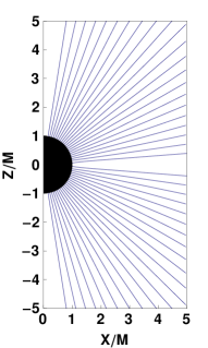
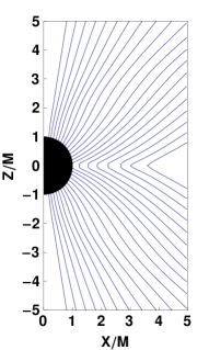
Figure 2: Left: Split monopole initial poloidal magnetic fields lines in blue (black in greyscale). Black shaded area designates the BH interior. Right: Same as in left, but at t = 5M.

The Faraday tensor $F_{\mu\nu}$ is given by Eqs. (27)–(31) of mg04 . They can be used to compute the electric field:

$$E_{i}=n^{\mu}F_{i\mu}=-\frac{1}{\alpha}F_{ti}+\frac{\beta^{j}}{\alpha}F_{ji},$$ (130)

where, for the Kerr-Schild metric in spherical coordinates,

$${\begin{split}\alpha=&\ \left(1+\frac{2Mr}{\Sigma}\right)^{-1/2},\beta^{r}=\frac{2Mr}{\Sigma+2Mr},\beta^{\theta}=\beta^{\phi}=0,\\ \sqrt{\gamma}\,=&\ \Sigma\sin\theta\sqrt{1+\frac{2Mr}{\Sigma}},\end{split}}$$ (131)

and where $\Sigma=r^{2}+a^{2}\cos^{2}\theta$. Finally,

$$E_{r} = -\frac{Ca^{3}}{8\alpha M^{3}}f^{\prime}(r)\cos\theta\sin^{2}\theta$$ (132)

$$E_{\theta} = -\frac{Ca}{8\alpha}[\sin\theta+a^{2}f(r)\sin\theta(2\cos^{2}\theta-\sin^{2}\theta)]$$ (134)

$$-\beta^{r}\sqrt{\gamma}\,\frac{aC}{8r^{2}}\left(1+\frac{4M}{r}\right)$$

$$E_{\phi} = \frac{\beta^{r}}{\alpha M}Ca^{2}f^{\prime}(r)\cos\theta\sin^{2}\theta.$$ (135)

Note that $f(r)\sim-r^{2}\ln r/4$ as $r\rightarrow\infty$, invalidating the solution at large $r$ (because $B^{2}<E^{2}$ at sufficiently large $r$). Following  k04 ; m06 we drop terms involving $f(r)$ and $f^{\prime}(r)$, making the solution accurate only to first order in $a_{*}$.

To perform the split monopole the constant $C$ is changed to $-C$ in the lower hemisphere ($\theta>\pi/2$), in the expressions of $B^{i}$ and $E^{i}$. The vector potential for the split monopole test then can be written as

$$A_{r} = -\frac{Ca}{8}|\cos\theta|\left(1+\frac{4M}{r}\right)\sqrt{1+\frac{2M}{r}}+O(a_{*}^{3})\qquad$$ (136)

$$A_{\phi} = C(1-|\cos\theta|)+O(a_{*}^{2}).$$ (137)

As pointed out in k04 , the split-monopole configuration is sensible only if there exists a conducting disc in the equatorial plane of the black hole to sustain it. Otherwise, the equatorial current sheet cannot be stable – the magnetic field lines will reconnect and be pushed away. If one assumes that the equatorial current sheet is stable, because it is sustained by a disk, then no reconnection is expected to take place. We can model both scenarios by turning off and on our resistivity prescription, i.e., the nulling of the inflow velocity in the current sheet. If we do null the inflow velocity into the equatorial current sheet, no reconnection takes place and our solution is in agreement with the solution found in m06 , as expected. The results of this test without the resistivity prescription are shown in Fig. 2, and are in good agreement with the ones obtained in k04 .

We perform this test setting $a_{*}=0.1$, and chose $r_{0}=1.0M$, so that the BH horizon corresponds to $r\approx 0.995M$ in the shifted KS radial coordinate. We perform this test on a fixed-mesh-refinement grid hierarchy with 6 levels of refinement setting the outer boundary at 100M. The half-side length of the refinement levels is $3.125\times 2^{6-n}M,\ \ n=1,2,\ldots,6$, $n=1$ indicating the coarsest level in the hierarchy. The resolution of each level is $\Delta x_{\min}\times 2^{6-n},\ \ n=1,2,\ldots,6$, where $\Delta x_{\min}$ is the resolution of the finest level. We use 3 resolutions $\Delta x_{\min}=M/8$, $\Delta x_{\min}=M/16$, and $\Delta x_{\min}=M/24$. The Courant factor is set to $0.03125\times 2^{n-1},\ n=1,\ldots,3$ and 0.5 for $n=4,5,6$. We use the generalized Lorenz gauge to run the test with damping parameter $\xi=4/M$. The solution shown in Fig. 2 corresponds to our low resolution run, and the results of all other resolutions are almost overlapping, indicating that the resolutions used are sufficiently high.

V.2.2 The Wald solution

The EM field of the solution to Maxwell’s equations in the electrovacuum about a black hole is generated by the 4-vector potential

$${\cal A}_{\mu}=\frac{B_{0}}{2}(\phi_{\mu}+2at_{\mu}),$$ (138)

where $B_{0}$ is a constant, $\phi^{\mu}=(\partial/\partial\phi)^{\mu}$ and $t^{\mu}=(\partial/\partial t)^{\mu}$.

In the Schwarzschild black hole case ($a=0$), this electrovacuum solution is also a force-free solution, which will be the case considered in this test. The 4-vector potential in this case is

$${\cal A}_{\mu}=\frac{B_{0}}{2}\phi_{\mu}.$$ (139)

The 3-vector potential is $A_{i}=B_{0}\phi_{i}/2=B_{0}g_{\phi i}/2$. In Kerr-Schild metric written in spherical coordinates, the only nonvanishing component is

$${A_{\phi}=\frac{B_{0}}{2}g_{\phi\phi}=\frac{B_{0}}{2}r^{2}\sin^{2}\theta.}$$ (140)

The magnetic field is given by

$$B^{i}=\epsilon^{ijk}\partial_{j}A_{k}=\frac{[ijk]}{\sqrt{\gamma}}\partial_{j}A_{k},$$ (141)

where $[ijk]$ denotes the antisymmetric permutation symbol. Hence the components of $B^{i}$ in spherical Kerr-Schild coordinates are

$$B^{r} = \frac{1}{\sqrt{\gamma}\,}\partial_{\theta}A_{\phi}=B_{0}\left(1+\frac{2M}{r}\right)^{-1/2}\cos\theta$$ (142)

$$B^{\theta} = -\frac{1}{\sqrt{\gamma}\,}\partial_{r}A_{\phi}=-\frac{B_{0}}{r}\left(1+\frac{2M}{r}\right)^{-1/2}\sin\theta$$ (143)

$$B^{\phi} = 0$$ (144)

$$B_{r} = B_{0}\cos\theta\sqrt{1+\frac{2M}{r}}$$ (145)

$$B_{\theta} = -B_{0}r\sin\theta\left(1+\frac{2M}{r}\right)^{-1/2}$$ (146)

$$B_{\phi} = 0$$ (147)

$$B^{2} = B_{0}^{2}\left(1-\frac{2M}{r+2M}\sin^{2}\theta\right).$$ (148)

As $r\rightarrow\infty$, $B^{i}$ becomes a uniform vector with magnitude $B_{0}$ and points in the $z$-direction. To compute $E^{i}$, first calculate

$${E_{i}=n^{\nu}F_{i\nu}=\frac{1}{\alpha}(F_{i0}-\beta^{j}F_{ij}).}$$ (149)

Given that $F_{i0}=\partial_{i}{\cal A}_{0}-\partial_{t}{\cal A}_{i}=\frac{B_{0}}{2}\partial_{i}\phi_{0}=\frac{B_{0}}{2}\partial_{i}g_{t\phi}=0$ and $F_{ij}=\partial_{i}A_{j}-\partial_{j}A_{i}$. The nonzero $F_{\mu\nu}$ components are

$${\begin{split}F_{r\phi}=&\ -F_{\phi r}=B_{0}r\sin^{2}\theta,\\ F_{\theta\phi}=&\ -F_{\phi\theta}=B_{0}r^{2}\sin\theta\cos\theta.\end{split}}$$ (150)

By use of Eq. (150), Eq. (149) yields

$$E_{r}=E_{\theta}=0\ \ \ ,\ \ \ E_{\phi}=2MB_{0}\left(1+\frac{2M}{r}\right)^{-1/2}\sin^{2}\theta,$$ (151)

and

$$E^{r} = E^{\theta}=0\ \ \ ,\ \ \ E^{\phi}=\frac{2MB_{0}}{r^{2}}\left(1+\frac{2M}{r}\right)^{-1/2}$$ (152)

$$E^{2} = \frac{4M^{2}B_{0}^{2}\sin^{2}\theta}{r^{2}}\left(1+\frac{2M}{r}\right)^{-1}.$$ (153)

The electric field vanishes as $r\rightarrow\infty$. It is now straightforward to see that ${\bf E}\cdot{\bf B}=0$ and $E^{2}<B^{2}$. Hence, this electrovacuum solution is also a force-free solution.

The 3-velocity can be calculated by

$${v^{i}=\alpha\frac{\epsilon^{ijk}E_{j}B_{k}}{B^{2}}-\beta^{i}=\frac{[ijk]E_{j}B_{k}}{B_{0}^{2}r\sin\theta(r+2M\cos^{2}\theta)}-\beta^{i}.}$$ (154)

and we find

$$v^{r} = -\frac{2M\cos^{2}\theta}{r+2M\cos^{2}\theta}$$ (155)

$$v^{\theta} = \frac{M\sin 2\theta}{r(r+2M\cos^{2}\theta)}$$ (156)

$$v^{\phi} = 0.$$ (157)

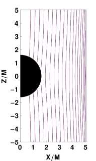
Figure 3: Poloidal magnetic field lines for the Schwarzchild electrovacuum Wald solution. Poloidal magnetic fields lines at $t=0$M in blue (black in greyscale), and at $t=5$M in red (grey in greyscale). Black shaded area designates the BH interior. The lines at $t=5$M are overlapping with those at $t=0$M.

For this test we arbitrarily chose $r_{0}=0.4M$, so that the BH horizon corresponds to $r=1.6M$ in the shifted KS radial coordinate. We perform this test on the same fixed-mesh-refinement grid hierarchy as the split-monopole test, using the same 3 resolutions and EM gauge. In Fig. 3 we show the Poloidal field lines at $t=0M$ and $t=5M$ for the low resolution run - the two overlap and cannot be distinguished by eye. Since this test is the only smooth 3D exact solution in the testbeds we consider we use it to also show that our code is convergent. Our convergence test study is presented in section Sec. V.4.

V.2.3 Magnetospheric Wald Problem

This again is a force-free problem. The initial data for the magnetic field are given by the same spatial vector potential as the Wald’s solution, i.e.,

$$A_{i}=\frac{B_{0}}{2}(\phi_{i}+2at_{i})=\frac{B_{0}}{2}(g_{i\phi}+2ag_{ti}).$$ (158)

However, the electric field is set to 0 initially, as in k04 . Hence $S_{i}=0$ and $v^{i}=-\beta^{i}$. There is no analytic solution to this problem. The evolution of the initial data is expected to reach a steady state similar to the one reported in k04 . Following k04 , we perform this test setting $a_{*}=0.9$. We also set $r_{0}=0.4359M$, so that the BH horizon lies at $r\approx 1.0M$ on our grid. We perform this test on the same fixed-mesh-refinement grid hierarchy as the other BH tests, using the same 3 resolutions and EM gauge. In Fig. 4 we plot the poloidal magnetic field lines at $t=126M$ at which point the solution has reached steady state and is very similar to that obtained in k04 .

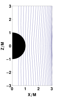
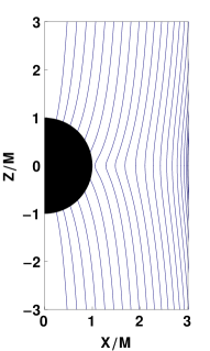
Figure 4: Left: Magnetospheric Wald initial poloidal magnetic fields lines in blue (black in greyscale). Black shaded area designates the BH interior. Right: Same as in left, but at t = 126M.

V.3 Force-free aligned rotator

Here we reproduce the aligned rotator, force-free solution in flat spacetime Contopoulos:1999ga ; Komissarov:2005xc ; McKinney:2006sd ; Spitkovsky:2006np . However, instead of applying the boundary condition on the NS surface, we use our new matching technique, which we described in Sec. IV.2.1, to evolve the magnetic field both interior and exterior to the star. In this approach the density profile of the star can be anything, as the magnetic field does not back-react onto the matter and an integration of the ideal MHD fluid equations is not performed. Instead, the density and velocity are evolved simply by “rotating” their initial values as described in  Paschalidis:2012ff . The density profile serves only as a proxy for locating the surface of the star. We endow the star with a uniform rotational three-velocity

$${\mathbf{v}=\Omega\mathbf{e}_{z}\times\mathbf{r},}$$ (159)

where $\mathbf{e}_{z}$ is the unit vector in the z-direction, and $\Omega$ is the stellar angular velocity. As in Spitkovsky:2006np we choose a spherical star and set $\Omega$ such that the theoretically expected location of the light cylinder radius, $R_{\rm LC}$, is 5 stellar radii away from the stellar center, i.e., $\Omega=1/5R_{\rm NS}$. In the exterior, the 3-velocity is set to 0. The electric field is set according to $\mbox{\boldmath$E$}=-\mbox{\boldmath$v$}\times\mbox{\boldmath$B$}$ everywhere and the Poynting vector is calculated using Eq. (18).

The star and its magnetosphere are endowed with a magnetic field corresponding to a dipole determined by the toroidal vector potential

$${A_{\phi}=\frac{\mu\varpi^{2}}{r^{3}},}$$ (160)

where $\mu=B_{p}R_{\rm NS}^{3}/2$ is the magnetic dipole moment, the cylindrical radial coordinate $\varpi^{2}=x^{2}+y^{2}$, and $r=\sqrt{x^{2}+y^{2}+z^{2}}$ is the radial coordinate.

We perform the test using 8 levels of refinement and set the outer boundary at $35.3R_{\rm LC}$. The length of each refinement box is $2.94R_{\rm NS}\times 2^{8-n},n=1,2,\ldots,8$, where $n=8$ corresponds to the finest refinement level. We use 3 resolutions: the low, medium and high resolutions cover the stellar radius with 34, 68 and 87 zones, respectively.

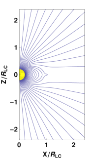
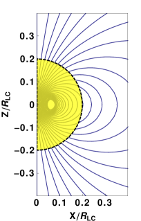
Figure 5: Left: Far field poloidal magnetic fields lines in blue (black in greyscale). Yellow (grey in greyscale) shaded area designates the stellar interior. Right: Same as in left, but zooming in on the near zone and showing the interior magnetic field, and how it smoothly joins to the exterior one. The time $t=6\pi/\Omega$, at which point the field has reached a stationary state.

Figure 6: Angular frequency of the magnetic field lines $\Omega_{F}$ normalized by the spin angular frequency of the star $\Omega$ vs the polar angle $\theta$ on the x-z plane for $r=0.3R_{\rm LC}$ (solid lines) and $r=0.7R_{\rm LC}$ (dashed lines). The value of this ratio should be unity. Two resolutions are shown here: low resolution (top) and high resolution (bottom). It is clear that the magnetosphere within the light cylinder is in near corotation with the star even for the low resolution case.

In Fig. 5 we show the poloidal magnetic field lines in the x-z plane, where it is clear that our code successfully captures the standard features of the pulsar magnetosphere: 1) the formation of a Y-point at the expected location of the light cylinder, 2) open field lines above the equatorial current sheet and beyond the light cylinder, and 3) dipole magnetic field structure within the light cylinder. In addition, the evolved interior field remains “frozen in” to the rotating matter. The right panel of the figure shows the structure of the magnetic field in the interior and the immediate exterior of the star, demonstrating that our matching technique is smooth.

The expected spin-down luminosity of an aligned rotator is $L=(1\pm 0.05)\mu^{2}\Omega^{4}$ Spitkovsky:2006np . We have calculated the outgoing EM radiation using the Poynting flux and the Penrose scalar $\phi_{2}$ (see e.g. Paschalidis:2013jsa ), and we find that it converges to a value within $4\%$ of $\mu^{2}\Omega^{4}$, and hence in good agreement with previous studies.

We plot the angular frequency of the magnetic field lines in the exterior bz77

$${\Omega_{F}(r,\theta)=\frac{F_{tr}}{F_{r\phi}}=\frac{F_{t\theta}}{F_{\theta\phi}},}$$ (161)

on the x-z plane at $r=0.3R_{\rm LC}$ and $r=0.7R_{\rm LC}$ as a function of the polar angle $\theta$. The result after $\sim 3$ periods of evolution is shown in Fig. 6 (cf. Komissarov:2005xc ; McKinney:2006sd who perform axisymmetric high-resolution simulations). It is clear that the magnetosphere within the light cylinder corotates with the star and that the higher the resolution, the closer is the magnetosphere to corotation.

V.4 Convergence

The Wald vector potential which generates the stationary magnetic field is itself time independent provided the proper electromagnetic gauge choice is made. A straightforward calculation demonstrates that

$${\begin{split}\epsilon_{ijk}v^{j}B^{k}=&\ \epsilon_{ijk}\bigg{(}\alpha\frac{\epsilon^{j\ell m}E_{\ell}B_{m}}{B^{2}}-\beta^{j}\bigg{)}B^{k}\\ =&\ -\alpha E_{i}-\epsilon_{ijk}\beta^{j}B^{k}\\ =&\ -\alpha E_{i}-\tilde{\epsilon}_{ijk}\tilde{\epsilon}^{k\ell m}\beta^{j}\partial_{\ell}A_{m}\\ =&\ -\alpha E_{i}-\beta^{j}(\partial_{i}A_{j}-\partial_{j}A_{i})\\ =&\ -\alpha E_{i}-\beta^{j}F_{ij}=0,\end{split}}$$ (162)

where in the first line we used Eq. (154), in the second line we used the degeneracy constraint (${\bf E}\cdot{\bf B}=0$), in the second and fourth lines we used the property $\epsilon_{ijk}\epsilon^{j\ell m}=(\delta_{i}{}^{\ell}\delta_{k}{}^{m}-\delta_{i}{}^{m}\delta_{k}{}^{\ell})$ and in the third line we used the definition $\tilde{B}^{k}=\tilde{\epsilon}^{k\ell m}\partial_{\ell}A_{m}$. The last equality in the fifth line holds true because of Eq. (149) and $F_{i0}=0$. This result implies that $\partial_{t}{\bf B}=0$ from the magnetic induction equation (76), but also has an interesting consequence regarding the typical electromagnetic gauges we use in our code: The evolution equation for the vector potential is given by Eq. (95). In the original algebraic electromagnetic gauge Etienne:2010ui $\alpha\Phi=\beta^{j}A_{j}$. Hence, the evolution equation (95) preserves the initial $A_{i}$ field ($\partial_{t}A_{i}=0$).

In fact, a straightforward calculation using the Wald vector potential shows that $\beta^{i}A_{i}=0$, which implies that the right-hand-side of Eq. (95) must be

$${\partial_{t}A_{i}=-\partial_{i}(\alpha\Phi)}$$ (163)

Thus, any electromagnetic gauge condition, for which $\partial_{i}(\alpha\Phi)=0$ will preserve the initial vector potential. Thus, the gauge $\alpha\Phi=\mbox{const.}$ also preserves the initial A-field.

Figure 7: Convergence test for the time-independence of the vector potential $A_{i}$. The plot shows the $L_{2}$ norms of the difference at $t=5$M between the numerical and analytic solutions in the volume contained inside a coordinate sphere of radius $r=90M$. The plot demonstrates that the error norms converge to zero as $\sim\Delta x^{2}$, i.e., the order of convergence of our code is 2. Note that $L_{2}(A_{x})\simeq 3.52\times 10^{4}$, so that $L_{2}(\Delta A_{x})/L_{2}(A_{x})\sim 10^{-6}$ even for the lowest-resolution run.

This is the case in the (generalized Lorenz) gauge UIUCEMGAUGEPAPER ; BriansLatest2012 we have developed, as we now demonstrate. The generalized Lorenz gauge is

$${\partial_{t}(\sqrt{\gamma}\Phi)+\partial_{j}(\alpha\sqrt{\gamma}A^{j})-\partial_{i}(\sqrt{\gamma}\beta^{i}\Phi)=-\xi\alpha\sqrt{\gamma}\Phi,}$$ (164)

where $\xi$ is the damping parameter. For the Wald solution $\partial_{j}(\alpha\sqrt{\gamma}A^{j})=0$, hence,

$${\partial_{t}(\sqrt{\gamma}\Phi)-\partial_{i}(\sqrt{\gamma}\beta^{i}\Phi)=-\xi\alpha\sqrt{\gamma}\Phi.}$$ (165)

This means that if $\Phi=0$ initially, $\partial_{t}\Phi=0$. Thus, even the generalized Lorenz gauge will preserve the Wald A-field (140), as long as the initial value for $\Phi$ is 0. Of course due to truncation error the right-hand-side of the evolution equation for $A_{i}$ will not be exactly 0, but will converge to 0 at second order which is the accuracy of our scheme.

A test of this convergence is shown in Fig. 7, where we plot the L2 norm of the difference between the numerical and analytic solution for the vector potential defined as

$${L_{2}(\Delta A_{i})=\sqrt{\int(A_{i}^{\rm num}-A_{i}^{\rm ex})^{2}d^{3}x},}$$ (166)

where $A_{i}^{\rm num},\ A_{i}^{\rm ex}$ designate the numerical and exact solutions, respectively. This norm should converge to 0 with increasing resolution. Fig.  7 demonstrates that our code is second-order convergent.

VI Summary

Neutron stars either in isolation or in compact binaries are likely to be endowed with a force-free magnetosphere. For inpiralling binaries, the GWs in the premerger regime can be accompanied by detectable “precursor” electromagnetic signals propagating through this magnetosphere. To study these effects numerical relativity simulations are necessary and require a scheme that matches the ideal MHD interior of the NS to the exterior force-free magnetosphere.

Here we present a new method for matching general relativistic ideal MHD to its force-free limit. We have tested out force-free code using a series of 1D flat spacetime tests, as well as 3D stationary black hole tests. We confirmed the validity of our new matching scheme by reproducing the well-known aligned rotator solution. We demonstrated the robustness of our algorithms and code and new techniques and we have shown that for smooth solutions our new code is second-order convergent.

This new method has already been used in Paschalidis:2013jsa , where we presented the first GR simulations of a binary black hole - neutron star magnetosphere. We plan to use this code to simulate other complicated dynamical spacetime scenarios involving neutron stars and their magnetospheres. In a future paper we also plan to extend our code to handle dynamical scenarios to extend our study to the inspiral of compact binaries involving neutron stars.

Appendix A Existence of a family of timelike vectors in GRFFE satisfying the ideal MHD condition

In this Appendix we demonstrate that the force-free conditions imply the ideal MHD condition.

Theorem: If the conditions (35) and (36) are satisfied, there exists a one-parameter family of timelike unit vectors $\{U^{\mu}\}$ so that $u_{\nu}\mathcal{F}^{\mu\nu}=0$ for any $u^{\mu}\in\{U^{\mu}\}$.

Proof: The proof can be established by finding the solution of the equation $u_{\mu}\mathcal{F}^{\mu\nu}=0$. If true, it follows that $0=u_{\mu}n_{\nu}\mathcal{F}^{\mu\nu}=u_{\mu}\mathcal{E}^{\mu}$. Substituting Eq. (8) for $\mathcal{F}^{\mu\nu}$ in $u_{\mu}\mathcal{F}^{\mu\nu}=0$ gives

$$\mathcal{E}^{\alpha}-v_{\beta}\mathcal{B}_{\gamma}n_{\delta}\epsilon^{\alpha\beta\gamma\delta}=0,$$ (167)

where $v^{\mu}=u^{\mu}/\gamma_{v}$ and $\gamma_{v}=-n_{\mu}u^{\mu}$. This is the GR version of the flat spacetime $\mbox{\boldmath$E$}+\mbox{\boldmath$v$}\times\mbox{\boldmath$B$}=0$ equation. We note that our Eq. (167) is different than Eq. (14) of m06 by a sign. We now prove the assertion by first decomposing $v^{\mu}$ in terms of 4 mutually orthogonal vectors $n^{\mu}$, $\mathcal{B}^{\mu}$, $\mathcal{E}^{\mu}$ and $\epsilon^{\mu\nu\alpha\beta}n_{\nu}\mathcal{B}_{\alpha}\mathcal{E}_{\beta}$:

$$v_{\beta}=G\left(\frac{-\epsilon_{\beta\mu\nu\lambda}n^{\mu}\mathcal{E}^{\nu}\mathcal{B}^{\lambda}}{B^{2}}\right)+Hn_{\beta}+K\left(\frac{\mathcal{E}_{\beta}}{\mathcal{E}}\right)+L\left(\frac{\mathcal{B}_{\beta}}{\mathcal{B}}\right),$$ (168)

where $G$, $H$, $K$ and $L$ are coefficients to be determined. It follows from $u_{\mu}\mathcal{E}^{\mu}=0$ and $v_{\mu}n^{\mu}=-1$ that $K=0$ and $H=1$. Substituting Eq. (168) into Eq. (167) and using $\mathcal{E}_{\mu}\mathcal{B}^{\mu}=0$ yields $G=1$. It follows from $u_{\mu}u^{\mu}=-1$ that $\gamma_{v}^{2}v_{\mu}v^{\mu}=-1$ or

$$\gamma_{v}=\sqrt{\frac{\mathcal{B}^{2}}{\mathcal{B}^{2}(1-L^{2})-\mathcal{E}^{2}}}.$$ (169)

Straightforward algebra also yields

$$\gamma_{v}=\sqrt{1+\gamma^{ij}u_{i}u_{j}}.$$ (170)

Since $\gamma^{ij}$ is positive-definite, $\gamma_{v}\geq 1$. Thus, in order for Eq. (169) to be a valid (real) solution, $L$ has to be restricted by

$$|L|<\sqrt{\frac{\mathcal{B}^{2}-\mathcal{E}^{2}}{\mathcal{B}^{2}}}.$$ (171)

With this restriction, Eq. (169) guarantees that $\gamma_{v}\geq 1$ since $\mathcal{B}^{2}>\mathcal{E}^{2}$. As a result the desired one-parameter family of unit timelike vectors is given by

$$u^{\mu}_{L}=\sqrt{\frac{\mathcal{B}^{2}}{\mathcal{B}^{2}(1-L^{2})-\mathcal{E}^{2}}}\left(n^{\mu}-\frac{\epsilon^{\mu\beta\gamma\delta}n_{\beta}\mathcal{E}_{\gamma}\mathcal{B}_{\delta}}{\mathcal{B}^{2}}+L\frac{\mathcal{B}^{\mu}}{\mathcal{B}}\right)$$ (172)

with the parameter $L$ taking values in the range given by Eq. (171). This completes the proof.

Note that the proof of the theorem depends crucially on the conditions (35) and (36), which imply $\mathcal{E}_{i}\mathcal{B}^{i}=0$ and $\mathcal{B}^{2}>\mathcal{E}^{2}$. The existence of a $u^{\mu}$ still holds, if (36) is replaced by $\mathcal{F}^{\mu\nu}\mathcal{F}_{\mu\nu}\geq 0$ with $\mathcal{F}^{\mu\nu}\mathcal{F}_{\mu\nu}=0$, if and only if $\mathcal{F}^{\mu\nu}=0$, in which case the condition $u_{\nu}\mathcal{F}^{\mu\nu}=0$ is automatically satisfied.

Appendix B Redundancy of the energy equation in the $S$-$\mathcal{B}$ formulation of GRFFE

In this appendix we demonstrate that the energy equation (82) is redundant because it can be derived from Eqs. (72), (74), (78) and (66).

Equations (72) and (74) are derived from the Maxwell Eq. (14) and Eq. (66). It is straightforward to show that Eqs. (72), (74) and (66) imply the Maxwell Eq. (14), which is also equivalent to Eq. (12). Combining the left equation of Eq. (11) and Eq. (17) yields

$${\nabla_{\nu}T_{\rm EM}^{\nu}{}_{\mu}=\mathcal{F}_{\nu\mu}\nabla_{\alpha}\mathcal{F}^{\nu\alpha}.}$$ (173)

It can also be shown that Eq. (78) implies

$${\nabla_{\nu}T_{\rm EM}^{\nu}{}_{i}=0.}$$ (174)

Hence, Eqs. (72),(74), (78) and (66) imply

$${\mathcal{F}_{\nu i}\nabla_{\alpha}\mathcal{F}^{\nu\alpha}=0.}$$ (175)

It remains to show Eq. (175) implies $\mathcal{F}_{\nu 0}\nabla_{\alpha}\mathcal{F}^{\nu\alpha}=0$.

Introduce the new quantities

$${\zeta=-n_{\nu}\nabla_{\alpha}\mathcal{F}^{\nu\alpha}}$$ (176)

and

$${Q^{\mu}=\gamma^{\mu}{}_{\nu}\nabla_{\alpha}\mathcal{F}^{\nu\alpha}.}$$ (177)

Then Eqs. (176) and (177) imply that

$${\nabla_{\alpha}\mathcal{F}^{\nu\alpha}=\zeta n^{\nu}+Q^{\nu}.}$$ (178)

Hence Eq. (175) via Eq. (178) and Eqs. (4), (5) yields

$$\zeta\mathcal{E}_{i}+\epsilon_{ijk}Q^{j}\mathcal{B}^{k}=0,$$ (179)

while

$${\begin{split}\mathcal{F}_{\nu 0}\nabla_{\alpha}\mathcal{F}^{\nu\alpha}=&\ \alpha(n^{\mu}\mathcal{F}_{\nu\mu}-n^{i}\mathcal{F}_{\nu i})\nabla_{\alpha}\mathcal{F}^{\nu\alpha}\\ =&\ \alpha n_{\mu}\mathcal{F}_{\nu}{}^{\mu}\nabla_{\alpha}\mathcal{F}^{\nu\alpha}\\ =&\ -\alpha^{2}\mathcal{F}_{\nu}{}^{0}\nabla_{\alpha}\mathcal{F}^{\nu\alpha}=\alpha\mathcal{E}_{i}Q^{i}.\end{split}}$$ (180)

Taking the cross product of Eq. (179) with $\mathcal{B}^{i}$ gives

$$\zeta\epsilon^{ijk}\mathcal{B}_{j}\mathcal{E}_{k}+\mathcal{B}^{2}Q^{i}-(Q^{j}\mathcal{B}_{j})\mathcal{B}^{i}=0.$$ (181)

Taking the dot product of Eq. (181) with $\mathcal{E}_{i}$ and using the degeneracy condition $\mathcal{E}_{i}\mathcal{B}^{i}=0$ [from Eq. (66)] and $\mathcal{B}^{2}\neq 0$ (otherwise the constraint $\mathcal{B}^{2}>\mathcal{E}^{2}$ will be violated) gives

$${\mathcal{E}_{i}Q^{i}=0.}$$ (182)

By virtue of Eq. (182) equation (180) implies

$${F_{\nu 0}\nabla_{\alpha}\mathcal{F}^{\nu\alpha}=0,}$$ (183)

which via Eq. (173) implies

$${\nabla_{\nu}T_{\rm EM}^{\nu}{}_{0}=0}$$ (184)

which equivalent to the energy equation (82). Thus, Eq. (82), as well as $\nabla_{\nu}T_{\rm EM}^{\mu\nu}=0$ and the condition $\mathcal{F}_{\nu\mu}\nabla_{\alpha}\mathcal{F}^{\nu\alpha}=0$, all follow from Eqs. (72), (74), (78), (66) plus the condition $\mathcal{B}^{2}\neq 0$. Hence the energy equation (82) is redundant .

Appendix C Evolution Equation for $C_{SB}$

In this appendix we derive the evolution equation for the constraint $C_{SB}=\mathcal{B}^{i}S_{i}$ using evolution equations (74) and (78). We demonstrate that the evolution equations preserve this constraint, provided it is satisfied initially.

It is convenient to write the EM stress-energy tensor in the form

$${\begin{split}T_{\rm EM}^{\mu\nu}=&\ \frac{\mathcal{B}^{2}+\mathcal{E}^{2}}{2}(\gamma^{\mu\nu}+n^{\mu}n^{\nu})-(\mathcal{B}^{\mu}\mathcal{B}^{\nu}+\mathcal{E}^{\mu}\mathcal{E}^{\nu})\\ &\ +n^{\mu}\bar{S}^{\nu}+n^{\nu}\bar{S}^{\mu},\end{split}}$$ (185)

where $\bar{S}^{\mu}=\gamma^{\mu\nu}S_{\nu}$. Recall that $\mathcal{E}^{\mu}$ is considered as a function of $S_{i}$ and $\mathcal{B}^{i}$ via

$$\mathcal{E}^{\mu}=\frac{\epsilon^{\mu\alpha\beta}\mathcal{B}_{\alpha}S_{\beta}}{\mathcal{B}^{2}}$$ (186)

and, hence, $\mathcal{B}_{\mu}\mathcal{E}^{\mu}=0$, but $\mathcal{B}^{\mu}S_{\mu}=C_{SB}$ is not set to 0 in this analysis. Define the purely spatial EM stress tensor according to:

$$\bar{T}_{\rm EM}^{\mu\nu}=\gamma^{\mu}{}_{\alpha}\gamma^{\nu}{}_{\beta}T_{\rm EM}^{\alpha\beta}=\frac{\mathcal{B}^{2}+\mathcal{E}^{2}}{2}\gamma^{\mu\nu}-(\mathcal{B}^{\mu}\mathcal{B}^{\nu}+\mathcal{E}^{\mu}\mathcal{E}^{\nu}),$$ (187)

where the components of $T_{\rm EM}^{\mu\nu}$ are

$$T_{\rm EM}^{00}=\frac{\mathcal{B}^{2}+\mathcal{E}^{2}}{2\alpha^{2}}\ \ \ ,\ \ \ T_{\rm EM}^{0j}=-\frac{\mathcal{B}^{2}+\mathcal{E}^{2}}{2\alpha^{2}}\beta^{j}+\frac{\bar{S}^{j}}{\alpha},$$ (188)

$${\begin{split}T_{\rm EM}^{j}{}_{i}=&\ \frac{\mathcal{B}^{2}+\mathcal{E}^{2}}{2}\delta^{j}{}_{i}-(\mathcal{B}^{j}\mathcal{B}_{i}+\mathcal{E}^{j}\mathcal{E}_{i})-\frac{\beta^{j}}{\alpha}S_{i}\\ =&\ \bar{T}_{\rm EM}^{j}{}_{i}-\frac{\beta^{j}}{\alpha}S_{i},\end{split}}$$ (189)

and where $\bar{T}_{\rm EM}^{j}{}_{i}\equiv\frac{\mathcal{B}^{2}+\mathcal{E}^{2}}{2}\delta^{j}{}_{i}-(\mathcal{B}^{j}\mathcal{B}_{i}+\mathcal{E}^{j}\mathcal{E}_{i})$. The following identities will be useful. For any purely spatial antisymmetric tensor $A^{ij}$ and purely spatial symmetric tensor $S^{ij}$,

$${\begin{split}D_{j}A^{ij}=&\ \frac{1}{\sqrt{\gamma}\,}\partial_{j}(\sqrt{\gamma}\,A^{ij}),\\ D_{j}S^{j}{}_{i}=&\ \frac{1}{\sqrt{\gamma}\,}\partial_{j}(\sqrt{\gamma}\,S^{j}{}_{i})-\frac{1}{2}S^{jk}\partial_{i}\gamma_{jk}.\end{split}}$$ (190)

Now, it follows from Eqs. (74) and (78) that

$$\partial_{t}(\gamma C_{SB}) = \partial_{t}(\tilde{\mathcal{B}}^{i}\tilde{S}_{i})=\sqrt{\gamma}\,S_{i}\partial_{t}\tilde{\mathcal{B}}^{i}+\sqrt{\gamma}\,\mathcal{B}^{i}\partial_{t}\tilde{S}_{i}$$ (193)

$$= -\sqrt{\gamma}\,S_{i}\partial_{j}\left(\alpha\sqrt{\gamma}\,\frac{\mathcal{B}^{i}\bar{S}^{j}-\mathcal{B}^{j}\bar{S}^{i}}{\mathcal{B}^{2}}\right.$$

$$+\sqrt{\gamma}\,\beta^{i}\mathcal{B}^{j}-\sqrt{\gamma}\,\beta^{j}\mathcal{B}^{i}\bigg{)}$$

$$-\sqrt{\gamma}\,\mathcal{B}^{i}\partial_{j}(\alpha\sqrt{\gamma}\,T_{\rm EM}^{j}{}_{i})+\frac{\alpha\gamma}{2}\mathcal{B}^{i}T_{\rm EM}^{\mu\nu}\partial_{i}g_{\mu\nu}$$

$$= X+Y,$$ (194)

where

$$X=-\alpha\gamma S_{i}D_{j}\left(\frac{\mathcal{B}^{i}\bar{S}^{j}-\mathcal{B}^{j}\bar{S}^{i}}{\mathcal{B}^{2}}\right)-\alpha\gamma\mathcal{B}^{i}D_{j}\bar{T}_{\rm EM}^{j}{}_{i},$$ (195)

and

$$Y = -\gamma S_{i}\frac{\mathcal{B}^{i}\bar{S}^{j}-\mathcal{B}^{j}\bar{S}^{i}}{\mathcal{B}^{2}}\partial_{j}\alpha$$ (198)

$$-\sqrt{\gamma}\,S_{i}\partial_{j}(\sqrt{\gamma}\,\beta^{i}\mathcal{B}^{j}-\sqrt{\gamma}\,\beta^{j}\mathcal{B}^{i})+\sqrt{\gamma}\,\mathcal{B}^{i}\partial_{j}(\sqrt{\gamma}\,\beta^{j}S_{i})$$

$$-\gamma\mathcal{B}^{i}T_{\rm EM}^{j}{}_{i}\partial_{j}\alpha+\frac{\alpha\gamma}{2}\mathcal{B}^{i}(T_{\rm EM}^{\mu\nu}\partial_{i}g_{\mu\nu}-\bar{T}_{\rm EM}^{jk}\partial_{i}\gamma_{jk})$$

$$= -\gamma\frac{\bar{S}^{j}\partial_{j}\alpha}{\mathcal{B}^{2}}C_{SB}+\gamma\frac{\bar{S}^{2}}{\mathcal{B}^{2}}\mathcal{B}^{j}\partial_{j}\alpha-\gamma S_{i}\beta^{i}C_{dB}-\gamma S_{i}\mathcal{B}^{j}\partial_{j}\beta^{i}$$ (205)

$$+\sqrt{\gamma}\,\partial_{j}(\sqrt{\gamma}\,\beta^{j})C_{SB}+\gamma S_{i}\beta^{j}\partial_{j}\mathcal{B}^{i}+\sqrt{\gamma}\,\partial_{j}(\sqrt{\gamma}\,\beta^{j})C_{SB}$$

$$+\gamma\mathcal{B}^{i}\beta^{j}\partial_{j}S_{i}-\gamma\mathcal{B}^{i}T_{\rm EM}^{j}{}_{i}\partial_{j}\alpha$$

$$+\frac{\alpha\gamma}{2}\mathcal{B}^{i}\bigg{[}T_{\rm EM}^{00}\partial_{i}g_{00}+2T_{\rm EM}^{0j}\partial_{i}g_{0j}$$

$$+\left(\frac{\mathcal{B}^{2}+\mathcal{E}^{2}}{2\alpha^{2}}\beta^{j}\beta^{k}-\frac{2\beta^{j}\bar{S}^{k}}{\alpha}\right)\partial_{i}\gamma_{jk}\bigg{]}.$$

The motivation for the separation of $X$ and $Y$ is that in the flat spacetime limit $Y=0$. We can now write some of the $Y$ terms as

$$\frac{\bar{S}^{2}}{\mathcal{B}^{2}}\mathcal{B}^{j}\partial_{j}\alpha=\left(\mathcal{E}^{2}+\frac{C_{SB}^{2}}{\mathcal{B}^{4}}\right)\mathcal{B}^{i}\partial_{i}\alpha.$$ (206)

$${\begin{split}S_{i}\mathcal{B}^{j}\partial_{j}\beta^{i}=&\ \mathcal{B}^{j}\partial_{j}(S_{i}\beta^{i})-\mathcal{B}^{j}\beta^{i}\partial_{j}S_{i}\\ =&\ \mathcal{B}^{i}\partial_{i}(\bar{S}^{j}\beta_{j})-\mathcal{B}^{i}\beta^{j}\partial_{i}S_{j}\\ =&\ \mathcal{B}^{i}\bar{S}^{j}\partial_{i}\beta_{j}+\mathcal{B}^{i}\beta_{j}\partial_{i}\bar{S}^{j}-\mathcal{B}^{i}\beta^{j}\partial_{i}S_{j}.\end{split}}$$ (207)

$$S_{i}\beta^{j}\partial_{j}\mathcal{B}^{i}=\beta^{i}\partial_{i}C_{SB}-\mathcal{B}^{i}\beta^{j}\partial_{j}S_{i}.$$ (208)

$$\mathcal{B}^{i}T_{\rm EM}^{j}{}_{i}\partial_{j}\alpha=\frac{\mathcal{E}^{2}-\mathcal{B}^{2}}{2}\mathcal{B}^{i}\partial_{i}\alpha-\frac{\beta^{i}}{\alpha}\partial_{i}\alpha C_{SB}.$$ (209)

$${\begin{split}\mathcal{B}^{i}T_{\rm EM}^{00}\partial_{i}g_{00}=&\ \frac{\mathcal{B}^{2}+\mathcal{E}^{2}}{2\alpha^{2}}\mathcal{B}^{i}\partial_{i}(-\alpha^{2}+\beta^{j}\beta_{j})\\ =&\ \frac{\mathcal{B}^{2}+\mathcal{E}^{2}}{2\alpha^{2}}\mathcal{B}^{i}(-2\alpha\partial_{i}\alpha+\beta^{j}\partial_{i}\beta_{j}+\beta_{j}\partial_{i}\beta^{j}).\end{split}}$$ (210)

$$\mathcal{B}^{i}T_{\rm EM}^{0j}\partial_{i}g_{0j}=-\frac{\mathcal{B}^{2}+\mathcal{E}^{2}}{2\alpha^{2}}\mathcal{B}^{i}\beta^{j}\partial_{i}\beta_{j}+\frac{\mathcal{B}^{i}\bar{S}^{j}}{\alpha}\partial_{i}\beta_{j}.$$ (211)

$${\begin{split}\mathcal{B}^{i}\beta^{j}\beta^{k}\partial_{i}\gamma_{jk}=&\ \mathcal{B}^{i}[\partial_{i}(\beta^{j}\beta_{j})-\gamma_{jk}\partial_{i}(\beta^{j}\beta^{k})]\\ =&\ \mathcal{B}^{i}(\beta^{j}\partial_{i}\beta_{j}-\beta_{j}\partial_{i}\beta^{j}).\end{split}}$$ (212)

$${\begin{split}\mathcal{B}^{i}\beta^{j}\bar{S}^{k}\partial_{i}\gamma_{jk}=&\ \mathcal{B}^{i}[\partial_{i}(\beta^{j}S_{j})-\gamma_{jk}\partial_{i}(\beta^{j}\bar{S}^{k})]\\ =&\ \mathcal{B}^{i}(\beta^{j}\partial_{i}S_{j}-\beta_{j}\partial_{i}\bar{S}^{j}).\end{split}}$$ (213)

Eqs. (206)-(213) imply

$$\frac{\alpha\gamma}{2}\mathcal{B}^{i}\left[T_{\rm EM}^{00}\partial_{i}g_{00}+2T_{\rm EM}^{0j}\partial_{i}g_{0j}+\left(\frac{\mathcal{B}^{2}+\mathcal{E}^{2}}{2\alpha^{2}}\beta^{j}\beta^{k}-\frac{2\beta^{j}\bar{S}^{k}}{\alpha}\right)\partial_{i}\gamma_{jk}\right]$$ (214)

(215)

$$=-\gamma\frac{\mathcal{B}^{2}+\mathcal{E}^{2}}{2}\mathcal{B}^{i}\partial_{i}\alpha+\gamma\mathcal{B}^{i}\bar{S}^{j}\partial_{i}\beta_{j}-\gamma\mathcal{B}^{i}(\beta^{j}\partial_{i}S_{j}-\beta_{j}\partial_{i}\bar{S}^{j}).$$

Gathering all the terms gives

$$Y = \partial_{i}(\gamma\beta^{i}C_{SB})+\gamma\left[\partial_{i}\beta^{i}-\left(\alpha\frac{\bar{S}^{i}}{\mathcal{B}^{2}}-\beta^{i}\right)\frac{\partial_{i}\alpha}{\alpha}\right]C_{SB}+\gamma\frac{\mathcal{B}^{i}\partial_{i}\alpha}{\mathcal{B}^{4}}C_{SB}^{2}-\gamma S_{i}\beta^{i}C_{dB}$$ (216)

$$= \partial_{i}(\gamma\beta^{i}C_{SB})+\gamma(\partial_{i}\beta^{i}-v^{i}a_{i})C_{SB}+\gamma\frac{\mathcal{B}^{i}\partial_{i}\alpha}{\mathcal{B}^{4}}C_{SB}^{2}-\gamma S_{i}\beta^{i}C_{dB},$$ (218)

where

$$a_{i}=n^{\mu}\nabla_{\mu}n_{i}=D_{i}(\ln\alpha)=\frac{\partial_{i}\alpha}{\alpha}$$ (219)

is the 4-acceleration of $n^{\mu}$.

The calculation of $X$ involves fewer algebraic operations:

$$\mathcal{B}^{i}D_{j}\bar{T}_{\rm EM}^{j}{}_{i} = \mathcal{B}^{i}D_{j}\left[\frac{\mathcal{B}^{2}+\mathcal{E}^{2}}{2}\delta^{j}{}_{i}-(\mathcal{B}^{j}\mathcal{B}_{i}+\mathcal{E}^{j}\mathcal{E}_{i})\right]$$ (220)

$$= \frac{\mathcal{B}^{i}}{2}D_{i}(\mathcal{B}^{2}+\mathcal{E}^{2})-\mathcal{B}^{i}D_{j}(\mathcal{B}^{j}\mathcal{B}_{i}+\mathcal{E}^{j}\mathcal{E}_{i})$$ (221)

$$= \mathcal{B}^{i}(\mathcal{B}^{j}D_{i}\mathcal{B}_{j}+\mathcal{E}^{j}D_{i}\mathcal{E}_{j})-\mathcal{B}^{i}\mathcal{B}^{j}D_{j}\mathcal{B}_{i}$$ (223)

$$-\mathcal{B}^{2}C_{dB}-\mathcal{B}^{i}\mathcal{E}^{j}D_{j}\mathcal{E}_{i}$$

$$= -\mathcal{B}^{2}C_{dB}+\mathcal{B}^{i}\mathcal{E}^{j}(D_{i}\mathcal{E}_{j}-D_{j}\mathcal{E}_{i})$$ (224)

$$= -\mathcal{B}^{2}C_{dB}+\mathcal{B}^{i}\mathcal{E}^{j}\delta^{lm}{}_{ij}D_{l}\mathcal{E}_{m}$$ (225)

$$= -\mathcal{B}^{2}C_{dB}+(\epsilon^{lmk}D_{l}\mathcal{E}_{m})(\epsilon_{ijk}\mathcal{E}^{j}\mathcal{B}^{i})$$ (226)

$$= -\mathcal{B}^{2}C_{dB}+(\epsilon^{lmk}D_{l}\mathcal{E}_{m})\epsilon_{ijk}\epsilon^{jpn}\mathcal{B}^{i}\frac{\mathcal{B}_{p}S_{n}}{\mathcal{B}^{2}}$$ (227)

$$= -\mathcal{B}^{2}C_{dB}+\frac{\epsilon^{lmk}D_{l}\mathcal{E}_{m}}{\mathcal{B}^{2}}\delta^{pn}{}_{ki}\mathcal{B}^{i}\mathcal{B}_{p}S_{n}$$ (228)

$$= -\mathcal{B}^{2}C_{dB}+\frac{\epsilon^{lmk}D_{l}\mathcal{E}_{m}}{\mathcal{B}^{2}}\mathcal{B}_{k}C_{SB}$$ (230)

$$-S_{k}\epsilon^{lmk}D_{l}\mathcal{E}_{m}.$$

Now

$$\epsilon^{lmk}D_{l}\mathcal{E}_{m} = \epsilon^{lmk}D_{l}\left(\epsilon_{mij}\frac{\mathcal{B}^{i}\bar{S}^{j}}{\mathcal{B}^{2}}\right)$$ (231)

$$= \delta^{kl}{}_{ij}D_{l}\left(\frac{\mathcal{B}^{i}\bar{S}^{j}}{\mathcal{B}^{2}}\right)=D_{l}\left(\frac{\mathcal{B}^{k}\bar{S}^{l}-\mathcal{B}^{l}\bar{S}^{k}}{\mathcal{B}^{2}}\right)$$ (233)

$$= D_{j}\left(\frac{\mathcal{B}^{k}\bar{S}^{j}-\mathcal{B}^{j}\bar{S}^{k}}{\mathcal{B}^{2}}\right).$$ (235)

By use of Eq. (235), Eq. (230) yields

$${\begin{split}\mathcal{B}^{i}D_{j}\bar{T}_{\rm EM}^{j}{}_{i}=&\ -\mathcal{B}^{2}C_{dB}+\mathcal{B}_{i}D_{j}\left(\frac{\mathcal{B}^{i}\bar{S}^{j}-\mathcal{B}^{j}\bar{S}^{i}}{\mathcal{B}^{2}}\right)C_{SB}\\ &\ -S_{i}D_{j}\left(\frac{\mathcal{B}^{i}\bar{S}^{j}-\mathcal{B}^{j}\bar{S}^{i}}{\mathcal{B}^{2}}\right)\end{split}}$$ (236)

and

$$X=\alpha\gamma\mathcal{B}^{2}C_{dB}-\alpha\sqrt{\gamma}\,\mathcal{B}_{i}\partial_{j}\left(\sqrt{\gamma}\,\frac{\mathcal{B}^{i}\bar{S}^{j}-\mathcal{B}^{j}\bar{S}^{i}}{\mathcal{B}^{2}}\right)C_{SB}.$$ (237)

Finally, using Eqs. (218) and (237) the evolution equation (194) becomes

$$\partial_{t}(\gamma C_{SB}) = \partial_{i}(\gamma\beta^{i}C_{SB})+\gamma(\partial_{i}\beta^{i}-v^{i}a_{i})C_{SB}$$ (241)

$$-\alpha\sqrt{\gamma}\,\mathcal{B}_{i}\partial_{j}\left(\sqrt{\gamma}\,\frac{\mathcal{B}^{i}\bar{S}^{j}-\mathcal{B}^{j}\bar{S}^{i}}{\mathcal{B}^{2}}\right)C_{SB}$$

$$+\gamma\frac{\mathcal{B}^{i}\partial_{i}\alpha}{\mathcal{B}^{4}}C_{SB}^{2}+\gamma(\alpha\mathcal{B}^{2}-S_{i}\beta^{i})C_{dB}.\qquad$$

Hence if $C_{SB}=C_{dB}=0$ initially, the evolution equations preserve the constraints.

Appendix D An alternative derivation for the FFE current

As in § III.3, $J^{i}$ can be decomposed into a parallel and a perpendicular components using Eqs. (54) and (55). The perpendicular component can be determined, as in § III.3, by taking the cross product of Eq. (37) with $\mathcal{B}^{i}$, resulting in the first equality of Eq. (56). It is straightforward to show that the remaining piece $\rho=D_{i}\mathcal{E}^{i}$, which is not a priori guaranteed in the $\mbox{\boldmath$S$}-\mbox{\boldmath$\mathcal{B}$}$ formulation, follows from the Maxwell equation $\nabla_{\nu}\mathcal{F}^{\mu\nu}=\mathcal{J}^{\mu}$.

$$\rho = -n_{\mu}\mathcal{J}^{\mu}=-n_{\mu}\nabla_{\nu}\mathcal{F}^{\mu\nu}$$ (242)

$$= -n_{\mu}\nabla_{\nu}(n^{\mu}\mathcal{E}^{\nu}-n^{\nu}\mathcal{E}^{\mu}-\epsilon^{\mu\nu\alpha\beta}\mathcal{B}_{\alpha}n_{\beta})$$ (243)

$$= \nabla_{\nu}\mathcal{E}^{\nu}+n_{\mu}n^{\nu}\nabla_{\nu}\mathcal{E}^{\mu}+\epsilon^{\mu\nu\alpha\beta}n_{\mu}\mathcal{B}_{\alpha}\nabla_{\nu}n_{\beta}$$ (244)

$$= (\delta_{\mu}{}^{\nu}+n_{\mu}n^{\nu})\nabla_{\nu}\mathcal{E}^{\mu}-\epsilon^{\mu\nu\alpha\beta}n_{\mu}\mathcal{B}_{\alpha}(K_{\nu\beta}+n_{\nu}a_{\beta})$$ (245)

$$= \gamma_{\mu}{}^{\nu}\nabla_{\nu}\mathcal{E}^{\mu}$$ (246)

$$= \gamma_{\mu}{}^{\nu}\delta^{\mu}{}_{\alpha}\nabla_{\nu}\mathcal{E}^{\alpha}$$ (247)

$$= \gamma_{\mu}{}^{\nu}(\gamma^{\mu}{}_{\alpha}-n^{\mu}n_{\alpha})\nabla_{\nu}\mathcal{E}^{\alpha}$$ (248)

$$= \gamma_{\mu}{}^{\nu}\gamma^{\mu}{}_{\alpha}\nabla_{\nu}\mathcal{E}^{\alpha}$$ (249)

$$= D_{\mu}\mathcal{E}^{\mu}$$

$$= D_{i}\mathcal{E}^{i},$$

which in terms of the $S_{i}$, $\mathcal{B}^{i}$ variables becomes

$${\rho=\epsilon^{ijk}D_{i}\left(\frac{\mathcal{B}_{j}S_{k}}{\mathcal{B}^{2}}\right).}$$ (251)

This takes care of the perpendicular component. The parallel component can be determined by computing the scalar $J_{\parallel}$:

$${\begin{split}J_{\parallel}=&\ \mathcal{B}_{\mu}\mathcal{J}^{\mu}=\mathcal{B}_{\mu}\nabla_{\nu}\mathcal{F}^{\mu\nu}\cr=&\ \mathcal{B}_{\mu}\nabla_{\nu}(n^{\mu}\mathcal{E}^{\nu}-n^{\nu}\mathcal{E}^{\mu}-\epsilon^{\mu\nu\alpha\beta}\mathcal{B}_{\alpha}n_{\beta})\cr=&\ \mathcal{B}_{\mu}\mathcal{E}^{\nu}\nabla_{\nu}n^{\mu}-\mathcal{B}_{\mu}n^{\nu}\nabla_{\nu}\mathcal{E}^{\mu}-\epsilon^{\mu\nu\alpha\beta}\mathcal{B}_{\mu}n_{\beta}\nabla_{\nu}\mathcal{B}_{\alpha}.\end{split}}$$ (252)

The last term in this last equation can be simplified

$$-\epsilon^{\mu\nu\alpha\beta}\mathcal{B}_{\mu}n_{\beta}\nabla_{\nu}\mathcal{B}_{\alpha} = n_{\beta}\mathcal{B}_{\mu}\epsilon^{\beta\mu\nu\alpha}\delta^{\gamma}{}_{\nu}\delta^{\lambda}{}_{\alpha}\nabla_{\gamma}\mathcal{B}_{\lambda}$$ (253)

$$= n_{\beta}\mathcal{B}_{\mu}\epsilon^{\beta\mu\nu\alpha}\gamma^{\gamma}{}_{\nu}\gamma^{\lambda}{}_{\alpha}\nabla_{\gamma}\mathcal{B}_{\lambda}$$ (254)

$$= n_{\beta}\mathcal{B}_{\mu}\epsilon^{\beta\mu\nu\alpha}D_{\nu}\mathcal{B}_{\alpha}$$ (255)

$$= \epsilon^{ijk}\mathcal{B}_{i}D_{j}\mathcal{B}_{k}.$$ (256)

The middle term in the last line of Eq. (252) can be rewritten using the Maxwell equation $\nabla_{\nu}{}^{*}\mathcal{F}^{\mu\nu}=0$, which implies

$${\begin{split}0=&\ \mathcal{E}_{\mu}\nabla_{\nu}{}^{*}\mathcal{F}^{\mu\nu}=\mathcal{E}_{\mu}\nabla_{\nu}(-n^{\mu}\mathcal{B}^{\nu}+n^{\nu}\mathcal{B}^{\mu}-\epsilon^{\mu\nu\alpha\beta}\mathcal{E}_{\alpha}n_{\beta})\cr=&\ -\mathcal{E}_{\mu}\mathcal{B}^{\nu}\nabla_{\nu}n^{\mu}+\mathcal{E}_{\mu}n^{\nu}\nabla_{\nu}\mathcal{B}^{\mu}-\epsilon^{\mu\nu\alpha\beta}n_{\beta}\mathcal{E}_{\mu}\nabla_{\nu}\mathcal{E}_{\alpha}\cr=&\ -\mathcal{E}^{\mu}\mathcal{B}^{\nu}\nabla_{\nu}n_{\mu}-n^{\nu}\mathcal{B}^{\mu}\nabla_{\nu}\mathcal{E}_{\mu}+n_{\beta}\epsilon^{\beta\mu\nu\alpha}\mathcal{E}_{\mu}\nabla_{\nu}\mathcal{E}_{\alpha},\cr\end{split}}$$ (257)

which yields

$${-\mathcal{B}_{\mu}n^{\nu}\nabla_{\nu}\mathcal{E}^{\mu}=\mathcal{E}^{\mu}\mathcal{B}^{\nu}\nabla_{\nu}n_{\mu}-\epsilon^{ijk}\mathcal{E}_{i}D_{j}\mathcal{E}_{k},}$$ (258)

where the identity $n_{\beta}\epsilon^{\beta\mu\nu\alpha}\mathcal{E}_{\mu}\nabla_{\nu}\mathcal{E}_{\alpha}=\epsilon^{ijk}\mathcal{E}_{i}D_{j}\mathcal{E}_{k}$ [which can be proved in a similar way as in Eq. (256)] has been used. Combining Eqs. (252)–(257) gives

$${\begin{split}J_{\parallel}=&\ \epsilon^{ijk}(\mathcal{B}_{i}D_{j}\mathcal{B}_{k}-\mathcal{E}_{i}D_{j}\mathcal{E}_{k})+\mathcal{E}^{\mu}\mathcal{B}^{\nu}(\nabla_{\nu}n_{\mu}+\nabla_{\mu}n_{\nu})\\ =&\ \epsilon^{ijk}(\mathcal{B}_{i}D_{j}\mathcal{B}_{k}-\mathcal{E}_{i}D_{j}\mathcal{E}_{k})-2\mathcal{E}^{i}\mathcal{E}^{j}K_{ij},\end{split}}$$ (259)

which is the same as Eq. (57). Hence the current density $J^{i}$ is given by Eq. (58), as expected.

References

- (1) S. Nissanke, M. Kasliwal, and A. Georgieva(2012), arXiv:1210.6362 [astro-ph.HE]
- (2) S. Rosswog, M. Liebendö Rfer, F.-K. Thielemann, and a. . P. l = http://adsabs.harvard.edu/abs/1998sese.conf..729R
- (3) S. Rosswog, M. Liebendoerfer, F. Thielemann, M. Davies, W. Benz, et al., Astron.Astrophys. 341, 499 (1999), arXiv:astro-ph/9811367 [astro-ph]
- (4) L.-X. Li and B. Paczynski, Astrophys.J. 507, L59 (1998), arXiv:astro-ph/9807272 [astro-ph]
- (5) S. Kulkarni(2005), arXiv:astro-ph/0510256 [astro-ph]
- (6) B. Metzger, G. Martinez-Pinedo, S. Darbha, E. Quataert, A. Arcones, et al.(2010), arXiv:1001.5029 [astro-ph.HE]
- (7) S. Goriely, A. Bauswein, and H.-T. Janka(2011), arXiv:1107.0899 [astro-ph.SR]
- (8) K. Hotokezaka, K. Kiuchi, K. Kyutoku, H. Okawa, Y.-i. Sekiguchi, et al., Phys.Rev. D87, 024001 (2013), arXiv:1212.0905 [astro-ph.HE]
- (9) K. Kyutoku, K. Ioka, and M. Shibata(2012), arXiv:1209.5747 [astro-ph.HE]
- (10) S. Rosswog, O. Korobkin, A. Arcones, and F. K. Thielemann(2013), arXiv:1307.2939 [astro-ph.HE]
- (11) D. Grossman, O. Korobkin, S. Rosswog, and T. Piran(2013), arXiv:1307.2943 [astro-ph.HE]
- (12) K. Kyutoku, K. Ioka, and M. Shibata(2013), arXiv:1305.6309 [astro-ph.HE]
- (13) A. Bauswein, S. Goriely, and H.-T. Janka, Astrophys.J. 773, 78 (2013), arXiv:1302.6530 [astro-ph.SR]
- (14) Z. B. Etienne, Y. T. Liu, S. L. Shapiro, and T. W. Baumgarte, Phys. Rev. D 79, 044024 (Feb. 2009)
- (15) M. D. Duez, F. Foucart, L. E. Kidder, C. D. Ott, and S. A. Teukolsky, Class.Quant.Grav. 27, 114106 (2010), arXiv:0912.3528 [astro-ph.HE]
- (16) M. Shibata, K. Kyutoku, T. Yamamoto, and K. Taniguchi, Phys.Rev. D79, 044030 (2009), arXiv:0902.0416 [gr-qc]
- (17) F. Foucart, M. D. Duez, L. E. Kidder, and S. A. Teukolsky, Phys.Rev. D83, 024005 (2011), arXiv:1007.4203 [astro-ph.HE]
- (18) K. Kyutoku, H. Okawa, M. Shibata, and K. Taniguchi, Phys.Rev. D84, 064018 (2011), arXiv:1108.1189 [astro-ph.HE]
- (19) B. C. Stephens, W. E. East, and F. Pretorius, Astrophys. J. Lett. 737, L5 (Aug. 2011), arXiv:1105.3175 [astro-ph.HE]
- (20) B. D. Lackey, K. Kyutoku, M. Shibata, P. R. Brady, and J. L. Friedman, Phys.Rev. D85, 044061 (2012), arXiv:1109.3402 [astro-ph.HE]
- (21) M. Shibata and K. Taniguchi, Living Reviews in Relativity 14 (2011), doi:“bibinfo–doi˝–10.12942/lrr-2011-6˝, http://www.livingreviews.org/lrr-2011-6
- (22) F. Foucart, M. B. Deaton, M. D. Duez, L. E. Kidder, I. MacDonald, et al.(2012), arXiv:1212.4810 [gr-qc]
- (23) W. E. East, F. Pretorius, and B. C. Stephens, Phys. Rev. D 85, 124009 (Jun. 2012), arXiv:1111.3055 [astro-ph.HE]
- (24) G. Lovelace, M. D. Duez, F. Foucart, L. E. Kidder, H. P. Pfeiffer, et al.(2013), arXiv:1302.6297 [gr-qc]
- (25) F. Foucart, L. Buchman, M. D. Duez, M. Grudich, L. E. Kidder, et al.(2013), arXiv:1307.7685 [gr-qc]
- (26) M. Shibata and K. Uryū, Progress of Theoretical Physics 107, 265 (Feb. 2002), arXiv:gr-qc/0203037
- (27) M. Shibata, K. Taniguchi, and K. Uryu, Phys.Rev. D68, 084020 (2003), arXiv:gr-qc/0310030 [gr-qc]
- (28) M. Shibata and K. Taniguchi, Phys.Rev. D73, 064027 (2006), arXiv:astro-ph/0603145 [astro-ph]
- (29) M. Anderson, E. W. Hirschmann, L. Lehner, S. L. Liebling, P. M. Motl, et al., Phys.Rev. D77, 024006 (2008), arXiv:0708.2720 [gr-qc]
- (30) L. Baiotti, B. Giacomazzo, and L. Rezzolla, Phys. Rev. D 78, 084033 (Oct. 2008), arXiv:0804.0594 [gr-qc]
- (31) L. Baiotti, B. Giacomazzo, and L. Rezzolla, Classical and Quantum Gravity 26, 114005 (Jun. 2009), arXiv:0901.4955 [gr-qc]
- (32) K. Kiuchi, Y. Sekiguchi, M. Shibata, and K. Taniguchi, Phys.Rev.Lett. 104, 141101 (2010), arXiv:1002.2689 [astro-ph.HE]
- (33) S. Bernuzzi, M. Thierfelder, and B. Brügmann, Phys. Rev. D 85, 104030 (May 2012), arXiv:1109.3611 [gr-qc]
- (34) J. A. Faber and F. A. Rasio, Living Reviews in Relativity 15 (2012), doi:“bibinfo–doi˝–10.12942/lrr-2012-8˝, http://www.livingreviews.org/lrr-2012-8
- (35) Y. Sekiguchi, K. Kiuchi, K. Kyutoku, and M. Shibata, Phys.Rev.Lett. 107, 051102 (2011), arXiv:1105.2125 [gr-qc]
- (36) V. Paschalidis, Z. B. Etienne, and S. L. Shapiro, Phys.Rev. D86, 064032 (2012), arXiv:1208.5487 [astro-ph.HE]
- (37) A. Bauswein, T. Baumgarte, and H. T. Janka(2013), arXiv:1307.5191 [astro-ph.SR]
- (38) S. Chawla, M. Anderson, M. Besselman, L. Lehner, S. L. Liebling, et al., Phys.Rev.Lett. 105, 111101 (2010)
- (39) Z. B. Etienne, Y. T. Liu, V. Paschalidis, and S. L. Shapiro, Phys. Rev. D 85, 064029 (Mar. 2012)
- (40) Z. B. Etienne, V. Paschalidis, and S. L. Shapiro, Phys. Rev. D 86, 084026 (Oct. 2012), arXiv:1209.1632 [astro-ph.HE]
- (41) M. Anderson, E. W. Hirschmann, L. Lehner, and Motl
- (42) Y. T. Liu, S. L. Shapiro, Z. B. Etienne, and K. Taniguchi, Phys.Rev. D78, 024012 (2008), arXiv:0803.4193 [astro-ph]
- (43) B. Giacomazzo, L. Rezzolla, and L. Baiotti, Phys. Rev. D 83, 044014 (Feb. 2011), arXiv:1009.2468 [gr-qc]
- (44) L. Rezzolla, B. Giacomazzo, L. Baiotti, J. Granot, C. Kouveliotou, et al., Astrophys.J. 732, L6 (2011), arXiv:1101.4298 [astro-ph.HE]
- (45) P. Goldreich and W. H. Julian, Astrophys.J. 157, 869 (1969)
- (46) B. M. Hansen and M. Lyutikov, Mon.Not.Roy.Astron.Soc. 322, 695 (2001), arXiv:astro-ph/0003218 [astro-ph]
- (47) S. T. McWilliams and J. Levin, Astrophys.J. 742, 90 (2011), arXiv:1101.1969 [astro-ph.HE]
- (48) M. Lyutikov, Phys.Rev. D83, 124035 (2011), arXiv:1104.1091 [astro-ph.HE]
- (49) A. L. Piro, Astrophys.J. 755, 80 (2012), arXiv:1205.6482 [astro-ph.HE]
- (50) D. Lai(2012), doi:“bibinfo–doi˝–10.1088/2041-8205/757/1/L3˝, arXiv:1206.3723 [astro-ph.HE]
- (51) D. J. D’Orazio and J. Levin(2013), arXiv:1302.3885 [astro-ph.HE]
- (52) P. Goldreich and D. Lynden-Bell, Astrophys. J. 156, 59 (Apr. 1969)
- (53) S. T. McWilliams and J. Levin, Astrophys. J. 742, 90 (Dec. 2011), arXiv:1101.1969 [astro-ph.HE]
- (54) K. Ioka and K. Taniguchi, Astrophys.J.(2000), arXiv:astro-ph/0001218 [astro-ph]
- (55) N. Bucciantini and L. Del Zanna(2012), arXiv:1205.2951 [astro-ph.HE]
- (56) K. Dionysopoulou, D. Alic, C. Palenzuela, L. Rezzolla, and B. Giacomazzo(2012), arXiv:1208.3487 [gr-qc]
- (57) C. Palenzuela, Mon. Not. R. Aston. Soc. 431, , 1853 (2), arXiv:1212.0130 [astro-ph.HE]
- (58) L. Lehner, C. Palenzuela, S. L. Liebling, C. Thompson, and C. Hanna, Phys.Rev. D86, 104035 (2012), arXiv:1112.2622 [astro-ph.HE]
- (59) V. Paschalidis, Z. B. Etienne, and S. L. Shapiro, Phys. Rev. D 88, 021504, (2013) (R), arXiv:1304.1805 [astro-ph.HE]
- (60) C. Palenzuela, L. Lehner, M. Ponce, S. L. Liebling, M. Anderson, et al.(2013), arXiv:1301.7074 [gr-qc]
- (61) C. Palenzuela, L. Lehner, S. L. Liebling, M. Ponce, M. Anderson, et al.(2013), arXiv:1307.7372 [gr-qc]
- (62) I. Contopoulos, D. Kazanas, and C. Fendt, Astrophys.J. 511, 351 (1999), arXiv:astro-ph/9903049 [astro-ph]
- (63) S. Komissarov, Mon.Not.Roy.Astron.Soc. 367, 19 (2006), arXiv:astro-ph/0510310 [astro-ph]
- (64) J. C. McKinney, Mon.Not.Roy.Astron.Soc.Lett. 368, L30 (2006), arXiv:astro-ph/0601411 [astro-ph]
- (65) A. Spitkovsky, Astrophys.J. 648, L51 (2006), arXiv:astro-ph/0603147 [astro-ph]
- (66) T. W. Baumgarte and S. L. Shapiro, Numerical Relativity: Solving Einstein’s Equations on the Computer (Cambridge University Press, 2010)
- (67) T. W. Baumgarte and S. L. Shapiro, Astrophys. J. 585, 921 (Mar. 2003), arXiv:astro-ph/0211340
- (68) M. D. Duez, Y. T. Liu, S. L. Shapiro, and B. C. Stephens, Phys.Rev. D72, 024028 (2005), arXiv:astro-ph/0503420 [astro-ph]
- (69) Z. B. Etienne, Y. T. Liu, and S. L. Shapiro, Phys.Rev. D82, 084031 (2010), arXiv:1007.2848 [astro-ph.HE]
- (70) Z. B. Etienne, V. Paschalidis, Y. T. Liu, and S. L. Shapiro, Phys. Rev. D 85, 024013 (Jan. 2012)
- (71) S. S. Komissarov, Mon. Not. Roy. Astron. Soc. 350, 427 (May 2004), arXiv:astro-ph/0402403
- (72) S. Komissarov, Mon.Not.Roy.Astron.Soc. 336, 759 (2002), arXiv:astro-ph/0202447 [astro-ph]
- (73) J. C. McKinney, Mon. Not. Roy. Astron. Soc. 367, 1797 (Apr. 2006), arXiv:astro-ph/0601410
- (74) R. D. Blandford and R. L. Znajek, Mon. Not. Roy. Astron. Soc. 179, 433 (May 1977)
- (75) S. S. Komissarov, Mon. Not. Roy. Astron. Soc. 418, L94 (Nov. 2011), arXiv:1108.3511 [astro-ph.HE]
- (76) R. M. Wald, Phys. Rev. D 10, 1680 (Sep. 1974)
- (77) S. S. Komissarov, Mon. Not. Roy. Astron. Soc. 336, 759 (Nov. 2002), arXiv:astro-ph/0202447
- (78) K. S. Thorne and D. MacDonald, Mon. Not. Roy. Astron. Soc. 198, 339 (Jan. 1982)
- (79) A. Gruzinov, ArXiv Astrophysics e-prints(Feb. 1999), arXiv:astro-ph/9902288
- (80) H. P. Pfeiffer and A. I. MacFadyen(2013), arXiv:1307.7782 [gr-qc]
- (81) G. Tóth, Journal of Computational Physics 161, 605 (2000), ISSN 0021-9991, http://www.sciencedirect.com/science/article/pii/S0021999100965197
- (82) C. R. Evans and J. F. Hawley, Astrophys. J. 332, 659 (Sep. 1988)
- (83) A. Dedner, F. Kemm, D. Kröner, C.-D. Munz, T. Schnitzer, and M. Wesenberg, Journal of Computational Physics 175, 645 (2002), ISSN 0021-9991, http://www.sciencedirect.com/science/article/pii/S002199910196961X
- (84) C. Palenzuela, T. Garrett, L. Lehner, and S. L. Liebling, Phys.Rev. D82, 044045 (2010), arXiv:1007.1198 [gr-qc]
- (85) D. Alic, P. Mosta, L. Rezzolla, O. Zanotti, and J. L. Jaramillo, Astrophys.J. 754, 36 (2012), arXiv:1204.2226 [gr-qc]
- (86) B. D. Farris, R. Gold, V. Paschalidis, Z. B. Etienne, and S. L. Shapiro, Phys.Rev.Lett. 109, 221102 (2012), arXiv:1207.3354 [astro-ph.HE]
- (87) P. Colella and P. R. Woodward, Journal of Computational Physics 54, 174 (Sep. 1984)
- (88) A. Harten, P. Lax, and B. van Leer, SIAM Rev. 25, 35 (1983)
- (89) Note that k02 ; k04 give the initial data for and . However, since the FFE equations are invariant if and are multiplied by a constant factor, initial data with and having the same values as the ones with and are equally valid and the subsequent evolution will be exactly the same as the old set of initial data after multiplying an appropriate factor. Therefore, the initial data listed in this note are not multiplied by the factor .
- (90) J. C. McKinney and C. F. Gammie, Astrophys. J. 611, 977 (Aug. 2004), arXiv:astro-ph/0404512
- (91) B. D. Farris, R. Gold, V. Paschalidis, Z. B. Etienne, and S. L. Shapiro, ArXiv e-prints(Jul. 2012), arXiv:1207.3354 [astro-ph.HE]
- (92) Note that we deliberately wrote instead of , instead of , and instead of . This is to demonstrate that the Maxwell equation is not needed to prove the redundancy of the energy equation.