Neutrinoless double beta decay of ⁴⁸Ca in the shell model: Closure versus nonclosure approximation

Abstract

Neutrinoless double-$\beta$ decay ($0\nu\beta\beta$) is a unique process that could reveal physics beyond the Standard Model. Essential ingredients in the analysis of $0\nu\beta\beta$ rates are the associated nuclear matrix elements. Most of the approaches used to calculate these matrix elements rely on the closure approximation. Here we analyze the light neutrino-exchange matrix elements of ⁴⁸Ca $0\nu\beta\beta$ decay and test the closure approximation in a shell-model approach. We calculate the $0\nu\beta\beta$ nuclear matrix elements for ⁴⁸Ca using both the closure approximation and a nonclosure approach, and we estimate the uncertainties associated with the closure approximation. We demonstrate that the nonclosure approach has excellent convergence properties which allow us to avoid unmanageable computational cost. Combining the nonclosure and closure approaches we propose a new method of calculation for $0\nu\beta\beta$ decay rates which can be applied to the $0\nu\beta\beta$ decay rates of heavy nuclei, such as ⁷⁶Ge or ⁸²Se.

I Introduction

Neutrinoless double-$\beta$ decay ($0\nu\beta\beta$), if observed, would prove that neutrinos are Majorana fermions, an important milestone in the search for physics beyond the Standard Model sv82 . In addition, one could extract more information about the nature of the decay mechanism and possibly determine the light neutrino mass hierarchy and the lightest neutrino mass ves12 ; tomoda , provided that the associated nuclear matrix elements (NME) are calculated with good accuracy ves12 ; prc13 ; prl13 ; prc10 ; prc07 .

There are many possible mechanisms that could contribute to the $0\nu\beta\beta$ decay process ves12 ; prc13 , and some of the associated matrix elements were investigated by using several approaches, including the quasiparticle random phase approximation (QRPA) ves12 , the interacting shell model prl100 ; prc13 , the interacting boson model iba-2 , the generator coordinate method gcm , and the projected Hartree-Fock Bogolibov model phfb . With the exception of the QRPA, all other methods entail using the closure approximation prc10 . Some older pv90 ; muto94 and more recent simvo11 analyses suggest that the deviation of the NME for the light neutrino-exchange mechanism from the closure approximation result should be small, but a full analysis of this deviation within the shell model is not yet available. In addition, the QRPA analysis is affected by uncertainties due to the $g_{pp}$ factor used to tune the residual interaction. For example, results from Ref. muto94 indicate a deviation of about up to 10% between closure and nonclosure NME, but its magnitude and sign depend on the choice of $g_{pp}$. The only shell-model analysis going beyond the closure approximation that we are aware of was done in Ref. pv90 for ⁴⁸Ca using a model space consisting of only the $f_{7/2}$ orbital. This model space is known to be insufficient for a good description of the NME due to the missing spin-orbit partner orbital $f_{5/2}$, which significantly reduces the Gamow-Teller strength. The authors of Ref. pv90 report very small changes of the NME from closure to nonclosure, and in most cases the magnitude of the nonclosure results is slightly smaller than the magnitude of the closure result.

In this paper we analyze and compare the closure and nonclosure NME for the $0\nu\beta\beta$ decay of ⁴⁸Ca using a shell-model approach in the full $pf$ shell prc10 ; prc13 . For the analysis we used the GXPF1A interaction gxpf1 ; gxpf1a . This analysis requires knowledge of a large number of one-body transition densities connecting the ground states of the initial and final states of ⁴⁸Ca and ⁴⁸Ti, respectively, with states of the intermediate nucleus ⁴⁸Sc. The total number of states in ⁴⁸Sc with angular momentum smaller than $J=7$ is about 100000. This is still an unmanageable task. However, we show that using only a few hundred states of each $J$ suffices to get accurate NME. In order to validate our results we also analyzed the $0\nu\beta\beta$ NME of the “fictitious” decays of ⁴⁴Ca and ⁴⁶Ca, for which a full account of all relevant states in the intermediate nucleus ⁴⁸Sc is possible. We find that the nonclosure NME always increases relative to its closure value by about 10%.

The paper is organized as follows. Section II gives a brief description of the light neutrino exchange $0\nu\beta\beta$ NME relevant for the distinction between the nonclosure approach and the closure approximation. Section III provides a brief description of the closure approximation. Section IV describes the approach we use to obtain the nonclosure results and outlines new mixed methods that use the closure approach to accelerate the convergence. In Sect. V we analyze the numerical results, and Sec. VI is devoted to conclusions and outlook. Details of the calculations are shown in the appendices.

II The nuclear matrix element

The decay rate for a $0\nu\beta\beta$ decay process, under the assumption that the light neutrino-exchange mechanism dominates ves12 ; prc13 , can be written as

$$\left[T^{0\nu}_{1/2}\right]^{-1}=G^{0\nu}|M^{0\nu}|^{2}\left(\frac{\langle m_{\beta\beta}\rangle}{m_{e}}\right)^{2}.$$ (1)

Here $G^{0\nu}$ is the phase-space factor kipf12 , $M^{0\nu}$ is the nuclear matrix element, and the effective neutrino mass $\langle m_{\beta\beta}\rangle$ is defined by the neutrino mass eigenvalues $m_{k}$ and the elements of neutrino mixing matrix $U_{ek}$ ves12 ,

$$\langle m_{\beta\beta}\rangle=\left|\sum_{k}m_{k}U^{2}_{ek}\right|.$$ (2)

The nuclear matrix element $M^{0\nu}$ is usually presented as a sum of Gamow-Teller (GT), Fermi (F), and Tensor (T) corr1 nuclear matrix elements (see, for example, Ref. prc10 ),

$$M^{0\nu}=M^{0\nu}_{GT}-\left(\frac{g_{V}}{g_{A}}\right)^{2}M^{0\nu}_{F}+M^{0\nu}_{T},$$ (3)

where $g_{V}$ and $g_{A}$ are the vector and axial constants correspondingly; in our calculations we use $g_{V}=1$ and $g_{A}=1.254$.

The nuclear matrix elements in Eq. (3) describe the transition from an initial nucleus $|i\rangle=|0^{+}_{i}\rangle$ to a final nucleus $|f\rangle=|0^{+}_{f}\rangle$, and they can be presented as a sum over intermediate nuclear states $|\kappa\rangle=|J^{\pi}_{\kappa}\rangle$ with certain angular momentum $J_{\kappa}$, parity $\pi$, and energy $E_{\kappa}$

$$M^{0\nu}_{\alpha}=\sum_{\kappa}\sum_{1234}\langle 13|{\cal O}_{\alpha}|24\rangle\langle f|\hat{c}^{\dagger}_{3}{\hat{c}}_{4}|\kappa\rangle\langle\kappa|\hat{c}^{\dagger}_{1}{\hat{c}}_{2}|i\rangle,$$ (4)

where operators ${\cal O}_{\alpha}$, $\alpha=\{GT,F,T\}$, contain neutrino potentials, spin and isospin operators, and the explicit dependence on the intermediate state energy $E_{\kappa}$. They are given by

$${\cal O}_{GT}= \tau_{1-}\tau_{2-}\;(\mbox{\boldmath{$\sigma$}}_{1}\cdot\mbox{\boldmath{$\sigma$}}_{2})\;H_{GT}(r,E_{\kappa}),$$ (5)

$${\cal O}_{F}= \tau_{1-}\tau_{2-}\;H_{F}(r,E_{\kappa}),$$

$${\cal O}_{T}= \tau_{1-}\tau_{2-}\;S_{12}\;H_{T}(r,E_{\kappa}),$$

with $S_{12}=3(\mbox{\boldmath{$\sigma$}}_{1}\cdot{\bf n})(\mbox{\boldmath{$\sigma$}}_{2}\cdot{\bf n})-(\mbox{\boldmath{$\sigma$}}_{1}\cdot\mbox{\boldmath{$\sigma$}}_{2})$, ${\bf r}={\bf r}_{1}-{\bf r}_{2}$, $r=|{\bf r}|$, and ${\bf n}={\bf r}/r$. The neutrino potentials, $H_{\alpha}(r,E_{\kappa})$, are integrals over the neutrino exchange momentum, $q$,

$$H_{\alpha}(r,E_{\kappa})=\frac{2R}{\pi}\int_{0}^{\infty}\frac{f_{\alpha}(qr)h_{\alpha}(q^{2})qdq}{q+E_{\kappa}-(E_{i}+E_{f})/2},$$ (6)

where $f_{GT,F}(qr)=j_{0}(qr)$ and $f_{T}(qr)=j_{2}(qr)$ are spherical Bessel functions. The nuclear radius $R=1.2\times A^{1/3}\,{\rm fm}$ was introduced to make the neutrino potentials dimensionless (and since the phase-space factor $G^{0\nu}$ contains $1/R^{2}$ the final transition probability does not depend on $R$). The form factors $h_{\alpha}(q^{2})$ are defined in Appendix A and they include vector and axial nucleon form factors that take into account nucleon size effects. Calculation details for two-body matrix elements, $\langle 13|{\cal O}_{\alpha}|24\rangle$, are discussed in Appendix D. Let us note that the two-body wave functions in the matrix elements (4) are not antisymmetrized, as one would expect for nuclear two-body matrix elements. They should be understood as

$$|24\rangle=|2\rangle\cdot|4\rangle\;\mbox{ and }\;|13\rangle=|1\rangle\cdot|3\rangle,$$ (7)

where 1, 2, 3, and 4 represent single-nucleon quantum numbers (for example, $1=\{\tau_{1z},n_{1},l_{1},j_{1},\mu_{1}\}$ and so on).

Appendices B, C, and D provide expressions for the nuclear matrix elements (4) by considering rotational symmetry and isospin invariance.

III The closure approximation

If one replaces the energies of the intermediate states in Eq. (6) by an average constant value one gets the closure approximation,

$$\left[E_{\kappa}-(E_{i}+E_{f})/2\right]\rightarrow\langle E\rangle.$$ (8)

The operators ${\cal O}_{\alpha}\rightarrow\tilde{{\cal O}}_{\alpha}\equiv{\cal O}_{\alpha}(\langle E\rangle)$ become energy independent and the sum over the intermediate states in the nuclear matrix element (4) can be taken explicitly by using the completeness relation

$$\sum_{\kappa}\langle f|\hat{c}^{\dagger}_{3}{\hat{c}}_{4}|\kappa\rangle\langle\kappa|\hat{c}^{\dagger}_{1}{\hat{c}}_{2}|i\rangle=\langle f|\hat{c}^{\dagger}_{3}{\hat{c}}_{4}\hat{c}^{\dagger}_{1}{\hat{c}}_{2}|i\rangle.$$ (9)

The advantage of this approximation is significant, because it eliminates the need of calculating a very large number of states in the intermediate nucleus, which could be computationally challenging, especially for heavy systems. One needs only to calculate the two-body transition densities (9) between the initial and the final nuclear states. This approximation is very good because the values of $q$ that dominate the matrix elements are of the order of $100-200$ MeV, while the relevant excitation energies are only of the order of 10 MeV. The obvious difficulty related to this approach is that we have to find a reasonable value for this average energy, $\langle E\rangle$, which can effectively represent the contribution of all the intermediate states. This average energy needs to account also for the symmetric part of the two-body matrix elements, $\langle 13|{\cal O}_{\alpha}|24\rangle$, in Eq. (4). Indeed, the two-body wave functions $|13\rangle$ and $|24\rangle$ are not antisymmetric; by replacing the energies of the intermediate states with a constant, only the antisymmetric part of these matrix elements is taken into account.

The uncertainty in the value of the nuclear matrix elements is related to our inability to derive the average energy, $\langle E\rangle$, associated with the closure approximation. Fortunately, the nuclear matrix elements are not very sensitive to the value of this average energy (with the uncertainty being estimated to be about 10%; see, for example, prc10 ). Such weak dependence on the average energy originates from the large value of typical momentum of the virtual neutrino [see Eq. (6)], which is $\sim 1\,{\rm fm}^{-1}$ ($\sim 200\,{\rm MeV}$), i.e., much larger than the typical nuclear excitations.

IV Nonclosure and mixed methods

In the nonclosure approach one needs to calculate the sum in Eq. (4) explicitly, which is an obvious challenge due to the large number of intermediate states $|\kappa\rangle$. For the case of ⁴⁸Ca in the $fp$ model space there are about $10^{5}$ intermediate states; it is extremely difficult to find and include all these states.

Let us introduce a cutoff energy $E$ to investigate the convergence of the sum over $\kappa$ in Eq. (4) (where here and below the sum over repeated indices $\{1,2,3,4\}$ is omitted):

$$M^{0\nu}_{\alpha}(E)=\sum_{E_{\kappa}<E}\langle 13|{\cal O}_{\alpha}|24\rangle\langle f|\hat{c}^{\dagger}_{3}{\hat{c}}_{4}|\kappa\rangle\langle\kappa|\hat{c}^{\dagger}_{1}{\hat{c}}_{2}|i\rangle.$$ (10)

Alternatively, we can use a cutoff on the number of states, $N$, calculating the sum only for $\kappa<N$. At the limit of large cutoff energies $M^{0\nu}_{\alpha}(E)$ approaches the exact value of the nuclear matrix element (4).

The difference between the closure and nonclosure calculations originates mainly from the low-lying excitation energies. The intermediate and higher energies cannot produce much of a difference, because with increase of the excitation energy the one-body matrix elements rapidly become very small. Based on this observation, we will use the nonclosure approach for low energies, which we can manage within the framework of the standard shell model. For the higher excitation energies, we will use the closure approximation, which is also manageable. To proceed further we introduce the sum similar to Eq. (10) for the closure approximation:

$${\cal M}^{0\nu}_{\alpha}(E)=\sum_{E_{\kappa}<E}\langle 13|\tilde{{\cal O}}_{\alpha}|24\rangle\langle f|\hat{c}^{\dagger}_{3}{\hat{c}}_{4}|\kappa\rangle\langle\kappa|\hat{c}^{\dagger}_{1}{\hat{c}}_{2}|i\rangle.$$ (11)

The difference between Eqs. (10) and (11) is that for the nonclosure approach the operators ${\cal O}_{\alpha}$ in Eq. (5) are functions of the excitation energy $E_{\kappa}$, while for the closure approximation the same operators $\tilde{{\cal O}}_{\alpha}$ are functions of the average energy $\langle E\rangle$ [see the energy substitution given by Eq. (8)]. At large cutoff energies, $E\rightarrow\infty$,

$${\cal M}^{0\nu}_{\alpha}(E)\rightarrow{\cal M}^{0\nu}_{\alpha}(\infty)=\langle 13|\tilde{{\cal O}}_{\alpha}|24\rangle\langle f|\hat{c}^{\dagger}_{3}{\hat{c}}_{4}\hat{c}^{\dagger}_{1}{\hat{c}}_{2}|i\rangle,$$ (12)

we get an “exact value” in the framework of the closure approximation.

To avoid disadvantages of both approaches we propose an interpolation method which combines both the nonclosure and closure approaches, by introducing the mixed NME

$${\bar{M}^{0\nu}_{\alpha}}(E)={M}^{0\nu}_{\alpha}(E)-{\cal M}^{0\nu}_{\alpha}(E)+{\cal M}^{0\nu}_{\alpha}(\infty).$$ (13)

We expect that this mixed NME, ${\bar{M}^{0\nu}_{\alpha}}(E)$, will converge much faster with the cutoff energy than the nonclosure, $M^{0\nu}_{\alpha}(E)$, and closure, ${\cal M}^{0\nu}_{\alpha}(E)$, matrix elements separately. At higher excitation energies these two NME will behave similarly, and the energy dependence will cancel out. We also expect that the mixed NME, Eq. (13), will have much weaker dependence on the average energy $\langle E\rangle$ than the pure closure NME; at least this dependence should weaken when the cutoff energy increases. It should be also mentioned that calculating ${\cal M}^{0\nu}_{\alpha}(E)$ and ${\bar{M}^{0\nu}_{\alpha}}(E)$ does not require more computational effort than calculating the energy-dependent nonclosure NME, $M^{0\nu}_{\alpha}(E)$, for a given energy cutoff. ${\cal M}^{0\nu}_{\alpha}(\infty)$ can be calculated by using Eq. (12) (the details of which are described in Ref. prc10 ).

V Results

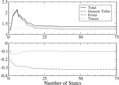
Figure 1: Convergence of closure NME ${\cal M}^{0\nu}_{\alpha}(E)$ with the number of intermediate states $|\kappa\rangle$ for the fictitious $0\nu\beta\beta$ decay of ⁴⁴Ca: Total (solid curve) and Gamow-Teller (dashed curve) (upper panel) and Fermi (dash-dotted curve) and Tensor (dotted curve) (lower panel).

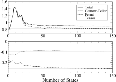
Figure 2: Same as Fig. 1 for the fictitious $0\nu\beta\beta$ decay of ⁴⁶Ca.

Figures 1 and 2 present the closure NME ${\cal M}^{0\nu}_{\alpha}(E)$ for the fictitious $0\nu\beta\beta$ decay cases of ⁴⁴Ca and ⁴⁶Ca. We calculated NME for these two cases only to demonstrate the convergence of the corresponding nuclear matrix elements with the increase of the cutoff energy. We could check our code by comparing with the NME calculated with a totally different method prc10 ; prc13 . The one-body transition densities ($\langle f|\hat{c}^{\dagger}_{3}{\hat{c}}_{4}|\kappa\rangle$ and $\langle\kappa|\hat{c}^{\dagger}_{1}{\hat{c}}_{2}|i\rangle$) were calculated with the NUSHELLX code nushellx , and we developed our code for the two-body matrix elements. We used the GXPF1A two-body interaction gxpf1 ; gxpf1a in the $pf$ model space. In the calculations we used $\langle E\rangle=7.72$ MeV, and we also included the short-range correlations (SRC) parametrization based on the AV18 potential and the standard nucleon finite-size effects prc10 . The horizontal lines represent the “exact values”, ${\cal M}^{0\nu}_{\alpha}(\infty)$. One can see how the NME converge to their exact values: for ⁴⁶Ca it is enough to take into account about 50 states (instead of $\sim 20\,000$) and for ⁴⁴Ca about 25 states are needed to obtain an accuracy better than 1% for the total NME. We should also mention that for ⁴⁴Ca and ⁴⁶Ca we were able to include all the states in the intermediate nucleus, and we got the same results as using the traditional nonclosure approach prc10 ; prc13 [see, e.g., Eq. (9)].

Figure 3 and Table 1 present the comparison of the results for the nonclosure approach, Eq. (11), with the closure NME, for the decay of ⁴⁸Ca. In these calculations we use

$$\left[E_{\kappa}-(E_{i}+E_{f})/2\right]\rightarrow 1.9\,{\rm MeV}+E^{*}_{\kappa},$$ (14)

where $E^{*}_{\kappa}$ is the excitation energy of the intermediate nucleus ⁴⁸Sc, the harmonic oscillator parameter $b_{osc}=1.989\,{\rm fm}$, and for the closure approximation the average energy was $\langle E\rangle=7.72\,{\rm MeV}$. Here, we also used the AV18 SRC parametrization prc10 . In Fig. 3 the nonclosure NME are represented by solid black and gray bars and the closure NME are the dashed bars, shown for various angular momenta $J_{\kappa}$ of intermediate states $|\kappa\rangle$. The Gamow-Teller matrix elements are all positive (upper part), and the Fermi matrix elements are all negative (bottom part). The main difference between closure and nonclosure comes from the GT nuclear matrix element corresponding to the intermediate angular momentum $J_{\kappa}=1$. The reason is that the transitions from an initial $0^{+}$ state to an intermediate $1^{+}$ state occur most naturally via the $\mbox{\boldmath{$\sigma$}}\tau_{-}$ operator. For the other types of operators and for the intermediate spins different from $J_{\kappa}=1$, we have to expand the form factors over the neutrino momentum $q$, which makes the nuclear matrix element insensitive to low excitation energies, and therefore does not contribute to the difference between closure and nonclosure NME. This decomposition of the matrix elements, which is often provided by QRPA calculations (see, e.g., Fig. 3 of Ref. qrpa-J ) is presented for the first time here as a result of a shell-model analysis. As mentioned in Ref. prc10 , there are no contributions from the negative-parity states of the intermediate nucleus when the model space is restricted to one major harmonic oscillator shell.

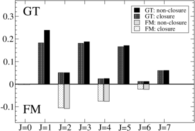
Figure 3: Nonclosure vs. closure GT and F nuclear matrix elements for $0\nu\beta\beta$ decay of ⁴⁸Ca for different spins $J$ of the intermediate states $|\kappa\rangle$. Solid black and gray bars correspond to the nonclosure approach, while shaded bars represent the closure approximation.

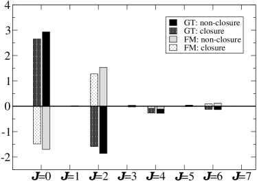
Figure 4: Nonclosure vs. closure GT and F nuclear matrix elements for $0\nu\beta\beta$ decay of ⁴⁸Ca calculated for certain spins of two initial neutrons and two final protons: $\langle 13,{\cal J}|{\cal O}^{\alpha}|24,{\cal J}\rangle$. The coloring scheme and parameters are the same as in Fig. 3.

Figure 4 represents another possible way to decouple the nuclear matrix elements. In this approach we consider two-body matrix elements $\langle 13|{\cal O}_{\alpha}|24\rangle$ where the single-particle states $|1\rangle$ and $|3\rangle$ (proton states) and the states $|2\rangle$ and $|4\rangle$ (neutron states) are coupled to certain common spin ${\cal J}$, so that the total NME can be presented as $M_{\alpha}=\sum_{\cal J}M_{\alpha}({\cal J})$. The details of such decoupling are in Appendix B. The nonclosure NME in Fig. 4 are represented with solid black and gray bars and the closure NME are the dashed bars. In contrast to the intermediate spin decoupling, where all the spins $J_{\kappa}$ contribute coherently (see Fig. 3), in the ${\cal J}$-decoupling scheme we see a significant cancellation between ${\cal J}=0$ and ${\cal J}=2$. Such a cancellation is responsible for the small matrix element of the double magic nucleus ⁴⁸Ca. Similar effects have been observed in seniority-truncation studies of the NME of ⁴⁸Ca menendez-sen (see also Ref. npa818 for effects of higher seniority in shell model calculations). QRPA results are available for heavier nuclei (see, e.g., Fig. 1 of Ref. qrpa-J ), for which the ${\cal J}=0$ and ${\cal J}=2$ contributions are still dominant, but the cancellation effect is significantly reduced.

Figure 5 presents the convergence of the total nuclear matrix element for ⁴⁸Ca to its final value, $100\%\times\delta M/M$, as a function of the cutoff energy. The solid line defined by Eq. (10) represents the nonclosure approach. We see that the matrix elements approach their final values (with the central shaded region corresponding to $\pm 1\%$) quite fast. In order to calculate the sum over the intermediate states in Eq. (4) within an accuracy better than 1% it is enough to include only the first 100 states for each $J_{\kappa}$. We conclude that if we restrict the sum over intermediate states to about 100 states of each spin, the uncertainty we introduce into the calculation by this restriction would be of the order of 1%.

The dotted and dashed lines in Fig. 5 represent the mixed method, where the NME are defined by Eq. (13). The dotted lines show the total matrix element, which includes all possible intermediate spins $J_{\kappa}$. It converges much faster than the pure nonclosure matrix element. To get an accuracy of about 1% using this method we have to take into account only states of up to 7 MeV in excitation energy (about 20 states per each $J_{\kappa}$). The hope is that using this mixed method we can achieve the desirable accuracy significantly faster (with a lower number of intermediate states) than using a pure nonclosure approach. To obtain the NME of heavier nuclei, for which the dimensions are extremely high, such a decrease in computational demands can be crucially important.

The main contribution to the NME originates from the intermediate states with spin $J_{\kappa}=1$ (see Fig. 3). This observation can be used to decrease the number of intermediate states required for a given accuracy. The dashed lines in Fig. 5 represent the NME when the intermediate sates with $J_{\kappa}=1$ are only taken into account. The difference between dotted and dashed lines is only 2%, which means that if we include only the first 20 states with $J_{\kappa}=1$ we already achieve an accuracy of 3%. This allows us to avoid calculation of all the intermediate states with $J_{\kappa}\neq 1$ and still get the NME with good accuracy.

Table 1 summarizes the difference between the total matrix elements calculated within the closure approximation and the nonclosure approach. We found about an 11% percent difference for the GT matrix element, which is quite noticeable. For the total matrix element this difference decreases to 10%.

The nonclosure results can be obtained in the closure approximation if one uses an appropriate value for $\langle E\rangle$ and not $\langle E\rangle=7.72$ MeV as suggested by QRPA calculations tomoda . For CD-Bonn and AV18 SRC parametrizations (see Table 2) this appropriate energy is found to be about $\langle E\rangle=0.5$ MeV, but its value may be different for different model spaces, interactions, or SRC parametrizations.

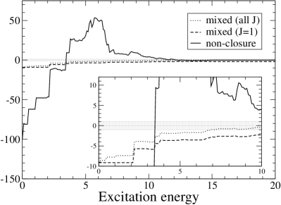
Figure 5: Convergence of total NME for $0\nu\beta\beta$ decay of ⁴⁸Ca to its final value, $100\%\times\delta M/M$, as a function of the cutoff energy. New mixed methods of calculation (presented by dotted and dashed lines) have much better convergence compared to the pure nonclosure approach (solid line). The insert shows the low-energy part.

	Closure	nonclosure	$\delta M/M$
Gamow-Teller, $M^{0\nu}_{GT}$	0.676	0.747	11%
Fermi, $M^{0\nu}_{F}$	-0.204	-0.208	2%
Tensor, $M^{0\nu}_{T}$	-0.077	-0.079	3%
Total, $M^{0\nu}$	0.729	0.800	10%

Table 1: Nonclosure vs closure nuclear matrix elements for $0\nu\beta\beta$ decay of ⁴⁸Ca calculated for the AV18 SRC parametrization and with closure average energy $\langle E\rangle=7.72$ MeV.

SRC	$M^{0\nu}_{GT}$	$M^{0\nu}_{F}$	$M^{0\nu}_{T}$	$M^{0\nu}$
None	0.782	-0.211	-0.077	0.839
Miller-Spencer	0.555	-0.143	-0.078	0.568
CD-Bonn	0.810	-0.226	-0.079	0.875
AV18	0.747	-0.208	-0.079	0.800

Table 2: Nonclosure nuclear matrix elements for $0\nu\beta\beta$ decay of ⁴⁸Ca calculated for different SRC parametrizations prc10 .

Finally, Table 2 presents the nonclosure ⁴⁸Ca NME calculations performed with different SRC parametrization sets prc10 .

VI Conclusions and Outlook

In conclusion, we investigated the closure versus nonclosure approach of the $0\nu\beta\beta$ NME for ⁴⁸Ca using for the first time shell-model techniques in the realistic $pf$ shell valence space. We found that the closure approximation always gives smaller NME, $M^{0\nu}_{\nu}$, by about 10%. A similar comparison of closure versus nonclosure NME for heavy nuclei, such as ⁷⁶Ge, ⁹⁶Zr, ¹⁰⁰Mo, and ¹³⁰Te, was done within the QRPA method in Ref. simvo11 (see, e.g., its Fig. 4), where the authors came to the same conclusion, namely, that the nonclosure NME are about 10% larger than the closure NME.

In addition, we were able to obtain for the first time a decomposition of the shell-model NME versus the total spin $J$ of the intermediate states, and we found that for the case of ⁴⁸Ca the $J=1$ states provide the largest contribution. We have also found that most of the additional difference between closure and nonclosure comes from the transitions to the $1^{+}$ states in the intermediate nucleus.

By combining the nonclosure and closure approaches together we propose a new method of calculating the $0\nu\beta\beta$ NME, which converges very quickly using only a very small number of states in the intermediate nucleus. This result suggests that one can apply this method to obtain the shell-model nonclosure NME for $0\nu\beta\beta$ decay of heavier nuclei, such as ⁷⁶Ge or ⁸²Se. It would be also interesting to go beyond the closure approximation for the NME corresponding to other mechanisms that may contribute to the $0\nu\beta\beta$ decay rates ves12 ; prc13 ; prl13 .

Finally, it is worth mentioning that the nonclosure approach does not constrain the states of the intermediate nucleus to be in the same model space used for the initial and the final state, as is the case for the closure approximation (see, e.g., Ref. prc10 ). For example, it was recently shown prl13 that the two-neutrino double-$\beta$ decay NME, which need to be calculated using a nonclosure approach, could change if the model space used for the intermediate $1^{+}$ states is enlarged. This effect could be considered in future studies. Here, we use for the nonclosure approach the same constraint as that imposed by the closure approximation.

RAS is grateful to N. Auerbach and V. Zelevinsky for constructive discussions. Support from the NUCLEI SciDAC Collaboration under U.S. Department of Energy Grant No. DE-SC0008529 is acknowledged. MH also acknowledges U.S. NSF Grant No. PHY-1068217.

Appendix A Form Factors

The form factors $h_{\alpha}(q^{2})$ in the neutrino potentials
given by Eq. (6) have the following form

$$h_{F}(q^{2})= \frac{g^{2}_{V}(q^{2})}{g^{2}_{V}},$$

$$h_{GT}(q^{2})= \frac{g^{2}_{A}(q^{2})}{g^{2}_{A}}\left[1-\frac{2}{3}\frac{q^{2}}{q^{2}+m^{2}_{\pi}}+\frac{1}{3}\left(\frac{q^{2}}{q^{2}+m^{2}_{\pi}}\right)^{2}\right]$$

$$+\frac{2}{3}\frac{g^{2}_{M}(q^{2})}{g^{2}_{A}}\frac{q^{2}}{4m^{2}_{p}},$$

$$h_{T}(q^{2})= \frac{g^{2}_{A}(q^{2})}{g^{2}_{A}}\left[\frac{2}{3}\frac{q^{2}}{q^{2}+m^{2}_{\pi}}-\frac{1}{3}\left(\frac{q^{2}}{q^{2}+m^{2}_{\pi}}\right)^{2}\right]$$

$$+\frac{1}{3}\frac{g^{2}_{M}(q^{2})}{g^{2}_{A}}\frac{q^{2}}{4m^{2}_{p}}.$$ (15)

Here $g_{V}=1$ and $g_{A}=1.254$ are the vector and axial constants and the form factors $g_{V,A,M}(q^{2})$ are given by

$$g_{V}(q^{2})= \frac{g_{V}}{(1+q^{2}/\Lambda^{2}_{V})^{2}},$$ (16)

$$g_{M}(q^{2})= (\mu_{p}-\mu_{n})g_{V}(q^{2}),$$

$$g_{A}(q^{2})= \frac{g_{A}}{(1+q^{2}/\Lambda^{2}_{A})^{2}},$$

where the finite-size parameters $\Lambda_{V}=850$ MeV, $\Lambda_{A}=1086$ MeV, and the magnetic moments $(\mu_{p}-\mu_{n})=4.7$.

Appendix B Nuclear Matrix Elements

The total matrix element of $0\nu\beta\beta$ decay, Eq. (4), is given by the sum over all the intermediate states $|\kappa\rangle$:

$$M^{0\nu}_{\alpha}=\sum_{\kappa}M^{\alpha}_{\kappa}.$$ (17)

We can introduce two different partial matrix elements, one of them corresponding to the sum over all intermediate states with certain spin $J_{\kappa}$,

$$M^{0\nu}_{\alpha}(J)=\mathop{\sum M^{\alpha}_{\kappa}}_{\kappa\;(J_{\kappa}=J)}\mbox{ and }\;M^{0\nu}_{\alpha}=\sum_{J}M^{0\nu}_{\alpha}(J),$$ (18)

and the other one corresponding to the sum over all intermediate states when the single-particle orbitals $|1\rangle$, $|3\rangle$ and $|2\rangle$, $|4\rangle$ in two-body matrix elements $\langle 13|{\cal O}_{\alpha}|24\rangle$ are coupled into total spin ${\cal J}$ as

$$|13,{\cal JM}\rangle=\sum_{m_{1}m_{3}}C^{\cal JM}_{j_{1}m_{1}\;j_{3}m_{3}}|j_{1}m_{1}\rangle|j_{3}m_{3}\rangle,$$ (19)

so that

$$M^{0\nu}_{\alpha}({\cal J})=\mathop{\sum M^{\alpha}_{\kappa}}_{\kappa\;({\cal J}={\rm fixed})}\mbox{ and }\;M^{0\nu}_{\alpha}=\sum_{{\cal J}}M^{0\nu}_{\alpha}({\cal J}).$$ (20)

The nuclear matrix elements, $M^{\alpha}_{\kappa}$, which we need for Eqs. (18) and (20), can be obtained from

$$M^{\alpha}_{\kappa}= f_{T}\sum_{1234}\left[(-1)^{j_{2}+j_{4}+{\cal J}}\Pi_{J_{\kappa}J_{\kappa}{\cal J}}\rule{0.0pt}{11.38092pt}\right.$$ (21)

$$\times\left\{\begin{array}[]{ccc}j_{1}&j_{2}&J_{\kappa}\\ j_{4}&j_{3}&{\cal J}\end{array}\right\}\langle 13,{\cal J}||{\cal O}_{\alpha}||24,{\cal J}\rangle$$

$$\left.\rule{0.0pt}{11.38092pt}\times\rho_{21}(J_{\kappa}\;t,i\rightarrow\kappa)\rho_{34}(J_{\kappa}\;t,f\rightarrow\kappa)^{*}\right],$$

where $\Pi_{ab\cdots z}=\sqrt{(2a+1)(2b+1)\cdots(2z+1)}$; operators ${\cal O}_{\alpha}$ are defined by Eq. (5) except for the isospin structure $\tau_{1-}\tau_{2-}$, which was taken into account separately by the isospin factor $f_{T}$; and $\rho_{21}$ and $\rho_{34}$ are the one-body transitional densities (OBTD) to be defined below. Note that the two-body matrix elements in the above equation are unsymmetrized.

Appendix C One-Body Transitional Densities

Nuclear initial, intermediate, and final states can be presented in the proton-neutron (PN) formalism or in the isospin (T) formalism.

In the PN formalism the nuclear states have certain isospin projection but no certain isospin. The isospin factor in this case simply equals one:

$$f_{T}=\langle p(1)p(3)|\tau_{1-}\tau_{2-}|n(2)n(4)\rangle=1.$$ (22)

For the OBTD we can ignore the isospin indices and get

$$\rho_{21}(J,i\rightarrow\kappa)=\frac{1}{\sqrt{2J+1}}\langle\kappa||[\hat{c}^{\dagger}_{1}\otimes\tilde{\hat{c}}_{2}]_{J}||i\rangle,$$ (23)

where the tilde denotes a time-conjugated state, $\tilde{\hat{c}}_{jm}=(-1)^{j+m}{\hat{c}}_{j-m}$.

In the T formalism, the nuclear states have certain isospin, which results in a non-trivial isospin factor,

$$f_{T}=-\frac{3}{2T_{\kappa}+1}{C^{T_{\kappa}{T_{\kappa}}_{z}}_{T_{f}{T_{f}}_{z}\,1+1}}{C^{T_{\kappa}{T_{\kappa}}_{z}}_{T_{i}{T_{i}}_{z}\,1-1}},$$ (24)

and a different definition of the OBTD,

$$\rho_{21}(Jt,i\rightarrow\kappa)=\frac{\langle\kappa|||[\hat{c}^{\dagger}_{1}\otimes\tilde{\hat{c}}_{2}]_{Jt}|||i\rangle}{\sqrt{2t+1}\sqrt{2J+1}},$$ (25)

where $\langle|||\cdots|||\rangle$ stands for the reduced matrix element in both spin and isospin spaces, and the time-conjugated state includes the additional factor $\tilde{\hat{c}}_{\frac{1}{2}\tau}=(-1)^{\frac{1}{2}+\tau}\hat{c}_{\frac{1}{2}-\tau}$.

Appendix D Reduced Matrix Elements

To calculate the reduced matrix elements in Eq. (21), $\langle 13,{\cal J}||{\cal O}_{\alpha}||24,{\cal J}\rangle$, we transform to relative and center-of-mass coordinates ${\bf r}={\bf r_{1}}-{\bf r_{2}}$ and ${\bf R}=({\bf r_{1}}+{\bf r_{2}})/2$. The operators ${\cal O}_{\alpha}$ depend only on relative coordinates, so let us rewrite these operators in such a form that will allow us to focus on the spin and coordinate dependencies (and for simplicity we omit here the isospin factor $\tau_{1-}\tau_{2-}$)

$${\cal O}_{\alpha}=\sum^{c}_{\gamma=-c}(-1)^{\gamma}\Sigma^{\alpha}_{c\,\;-\gamma}\left\langle{{\cal A}^{\alpha}_{c\;\gamma}(q,{\bf r})}\right\rangle_{\kappa},$$ (26)

where $c=0$ for $\alpha=\{GT,F\}$ and $c=2$ for $\alpha=T$. Here $\Sigma^{\alpha}_{c\;\gamma}$ include all the spin dependence as

$$\Sigma^{GT}_{00}=(\mbox{\boldmath{$\sigma$}}_{1}\cdot\mbox{\boldmath{$\sigma$}}_{2}),\;\;\Sigma^{F}_{00}=1,\;\;\Sigma^{T}_{2\gamma}=\left[\sigma_{1}\otimes\sigma_{2}\right]_{2\gamma},$$ (27)

${\cal A}^{\alpha}_{c\;\gamma}$ carry the coordinate and $q$ dependence as

$${\cal A}^{GT}_{0\;0}(q,{\bf r})={\cal A}^{F}_{0\;0}(q,{\bf r})=j_{0}(qr),$$ (28)

$${\cal A}^{T}_{2\;\gamma}(q,{\bf r})=\sqrt{\frac{24\pi}{5}}j_{2}(qr)Y_{2\gamma}({\bf n}),$$

and the average over neutrino momentum $q$ means

$$\left\langle\rule{0.0pt}{9.38945pt}{\cal T}^{\alpha}(q)\right\rangle_{\kappa}=\frac{2R}{\pi}\int{\cal T}^{\alpha}(q)\frac{h_{\alpha}(q^{2})\,qdq}{q+E_{\kappa}-(E_{i}+E_{f})/2},$$ (29)

where ${\cal T}^{\alpha}(q)$ is an arbitrary function of $q$ that has a certain index $\alpha=\{GT,F,T\}$, so that each function ${\cal T}^{\alpha}(q)$ is averaged with its own form factor $h_{\alpha}(q^{2})$. Now, omitting the average over the neutrino momentum, we can present the reduced matrix elements as

$$\langle 13,{\cal J}|| \sum^{c}_{\gamma=-c}(-1)^{\gamma}\Sigma^{\alpha}_{c\,\;-\gamma}{\cal A}^{\alpha}_{c\;\gamma}(q,{\bf r})||24,{\cal J}\rangle$$ (30)

$$=\Pi_{\cal J}\sum C_{13}C_{24}(-1)^{S+\lambda^{\prime}+{\cal J}}$$

$$\times\left\{\begin{array}[]{ccc}S^{\prime}&S&c\\ \lambda&\lambda^{\prime}&{\cal J}\end{array}\right\}\langle S||\Sigma^{\alpha}_{c}||S^{\prime}\rangle\langle\lambda||{\cal A}^{\alpha}_{c}||\lambda^{\prime}\rangle,$$

where the coefficients $C_{13}$ and $C_{24}$ are responsible for coupling the nucleon individual spins and angular momenta to certain common spin and angular momentum:

$$C_{13}=\langle S\lambda;{\cal J}|l_{1}j_{1},l_{3}j_{3};{\cal J}\rangle,$$ (31)

$$C_{24}=\langle S^{\prime}\lambda^{\prime};{\cal J}|l_{2}j_{2},l_{4}j_{4};{\cal J}\rangle.$$

They can be easily calculated from

$$C_{13}=\Pi_{j_{1}j_{3}\lambda S}\left\{\begin{array}[]{ccc}\frac{1}{2}&l_{3}&j_{3}\\ \frac{1}{2}&l_{1}&j_{1}\\ S&\lambda&{\cal J}\end{array}\right\},$$ (32)

$$C_{24}=\Pi_{j_{2}j_{4}\lambda^{\prime}S^{\prime}}\left\{\begin{array}[]{ccc}\frac{1}{2}&l_{4}&j_{4}\\ \frac{1}{2}&l_{2}&j_{2}\\ S^{\prime}&\lambda^{\prime}&{\cal J}\end{array}\right\}.$$

Calculation of the spin reduced matrix element in Eq. (30) is straightforward, but the radial and angular parts require more attention. To transform to relative coordinate we need to use Talmi-Moshinsky brackets $D_{13}$ and $D_{24}$

$$\langle 13,\lambda||{\cal A}^{\alpha}_{c}||24,\lambda^{\prime}\rangle=\Pi_{\lambda\lambda^{\prime}}\sum D_{13}D_{24}(-1)^{L+\lambda^{\prime}+l_{r}}$$ (33)

$$\times\left\{\begin{array}[]{ccc}l_{r}^{\prime}&l_{r}&c\\ \lambda&\lambda^{\prime}&L\end{array}\right\}\langle n_{r}l_{r}||{\cal A}^{\alpha}_{c}||n_{r}^{\prime}l_{r}^{\prime}\rangle,$$

where the sum runs over all allowed center-of-mass and relative radial and angular quantum numbers: $\{N,L\}$, $\{n_{r},l_{r}\}$, and $\{n_{r}^{\prime},l_{r}^{\prime}\}$. Coefficients $D_{13}$ and $D_{24}$ perform transformation of the orbital wave functions to the relative and center-of-mass wave functions

$$|n_{1}l_{1},n_{3}l_{3};\lambda\rangle=\sum_{n_{r}l_{r},NL}D_{13}|n_{r}l_{r},NL;\lambda\rangle,$$ (34)

$$|n_{2}l_{2},n_{4}l_{4};\lambda^{\prime}\rangle=\sum_{n_{r}^{\prime}l_{r}^{\prime},NL}D_{24}|n_{r}^{\prime}l_{r}^{\prime},NL;\lambda^{\prime}\rangle.$$

The angular reduced matrix elements in Eq. (33) have a standard form and can be found with the help of Ref. varsh , and the radial part of the reduced matrix elements can be integrated analytically, which allows us to significantly increase the accuracy and efficiency of the calculations. Indeed, the radial matrix elements we are interested in Eq. (33) are

$$\langle n_{r}l_{r}|j_{l}(qr)|n_{r}^{\prime}l_{r}^{\prime}\rangle$$ (35)

$$=\int_{0}^{\infty}R_{n_{r}l_{r}}(r)j_{l}(qr)R_{n_{r}^{\prime}l_{r}^{\prime}}(r)r^{2}dr,$$

with $l=0,2$. They can be reduced to a sum of table integrals (see for example ryzhik , p. 730, Eq. (6.631))

$${\nu}^{\frac{m+1}{2}}\int_{0}^{\infty}r^{m}e^{-\nu r^{2}}j_{l}(qr)dr$$

$$=\frac{\sqrt{\pi}}{4}k!z^{{l}/{2}}L^{(l+\frac{1}{2})}_{k}(z)e^{-z},$$ (36)

where $k=(m-l-2)/2$ (and in our case $k$ is always an integer and positive), $z=q^{2}/4\nu$, and $L^{(l+\frac{1}{2})}_{k}(z)$ are generalized Laguerre polynomials. To use these integrals one needs to expand the radial wave function, $R_{nl}$, in Eq. (35). We used the standard expansion of generalized Laguerre polynomials

$$L^{(\beta)}_{n}(\nu r^{2})=\sum_{i=0}^{n}\left(\begin{array}[]{c}\beta+n\\ n-i\end{array}\right)\frac{(-\nu r^{2})^{i}}{i!}.$$ (37)

The short range correlations are included by introducing the correlation function $f(r)$ that modifies the relative radial wave function at short distances (see, for example, Ref. prc10 ),

$$R_{n_{r}l_{r}}(r)\rightarrow[1+f(r)]R_{n_{r}l_{r}}(r).$$ (38)

The function $f(r)=-ce^{-ar^{2}}(1-br^{2})$ is parametrized in such a way that we can still integrate analytically the radial matrix elements with the help of relation (D) (see prc86 and references therein).

Finally, the integration over the neutrino momentum $q$ was performed numerically by using Gauss-Laguerre and Gauss-Legendre quadrature rules.

References

- (1) J. Schechter and J.W.F. Valle, Phys. Rev. D 25, 2951 (1982).
- (2) J.D. Vergados, H. Ejiri, and F. Simkovic, Rep. Prog. Phys. 75, 106301 (2012).
- (3) T. Tomoda, Rep. Prog. Phys. 54, 53 (1991).
- (4) M. Horoi, Phys. Rev. C 87, 014320 (2013).
- (5) M. Horoi and B.A. Brown, Phys. Rev. Lett. 110, 222502 (2013).
- (6) M. Horoi and S. Stoica, Phys. Rev. C 81, 024321 (2010).
- (7) M. Horoi, S. Stoica, B.A. Brown, Phys. Rev. C 75, 034303 (2007).
- (8) E. Caurier, J. Menendez, F. Nowacki, and A. Poves, Phys. Rev. Lett. 100, 052503 (2008).
- (9) J. Barea and F. Iachello, Phys. Rev. C 79, 044301 (2009); J. Barea, J. Kotila, and F. Iachello, Phys. Rev. Lett. 109, 042501 (2012).
- (10) T.R. Rodriguez and G. Martinez-Pinedo, Phys. Rev. Lett. 105, 252503 (2010).
- (11) P.K. Rath, R. Chandra, K. Chaturvedi, P.K. Raina, and J.G. Hirsch, Phys. Rev. C 82, 064310 (2010).
- (12) G. Pantis and J.D. Vergados, Phys. Lett. B 242, 1 (1990).
- (13) K. Muto, Nucl. Phys. A 577, 415c (1994).
- (14) F. Simkovic, R. Hodak, A. Faessler, and P. Vogel, Phys. Rev. C83, 015502 (2011).
- (15) M. Honma, T. Otsuka, B.A. Brown, and T. Mizusaki, Phys. Rev. C 69, 034335 (2004).
- (16) M. Honma, T. Otsuka, B.A. Brown, and T. Mizusaki, Eur. Phys. J. A 25, Suppl. 1, 499 (2005).
- (17) J. Kotila and F. Iachello, Phys. Rev. C 85, 034316 (2012).
- (18) The small tensor term in Ref. prc13 has the opposite sign.
- (19) http://www.garsington.eclipse.co.uk/ .
- (20) F. Simkovic, A. Faessler, V. Rodin, P. Vogel, and J. Engel, Phys. Rev. C 77, 045503 (2008).
- (21) J. Menendez, talk presented at the INT Program “Nuclei and Fundamental Symmetries”, INT Seattle, August 5-30, 2013.
- (22) J. Menendez, A. Poves, E. Caurier, and F. Nowacki, Nucl. Phys. A 818, 139 (2009).
- (23) D. Varshalovich, A. Moskalev, V. Khersonskii, Quantum Theory of Angular Momentum (World Scientific, Singapore, 1988).
- (24) I.S. Gradshteyn, I.M. Ryzhik, Table of Integrals, Series and Products (Academic, New York, 1980).
- (25) A. Neacsu, S. Stoica, and M. Horoi, Phys. Rev. C 86, 067304 (2012).