forqs: Forward-in-time Simulation of Recombination, Quantitative Traits, and Selection

Abstract

Summary: forqs is a forward-in-time simulation of recombination, quantitative traits, and selection. It was designed to investigate haplotype patterns resulting from scenarios where substantial evolutionary change has taken place in a small number of generations due to recombination and/or selection on polygenic quantitative traits.

Availability and Implementation: forqs is implemented as a command-line C++ program. Source code and binary executables for Linux, OSX, and Windows are freely available under a permissive BSD license:
https://bitbucket.org/dkessner/forqs

Contact: jnovembre@uchicago.edu, dkessner@ucla.edu

1 Introduction

Simulations have a long history in population genetics, both for verifying analytical results and for exploring population models that are mathematically intractable. Population genetics simulations can be broadly classified as forward-in-time (e.g. Wright-Fisher) or backward-in-time (e.g. coalescent). Coalescent simulations (e.g. ms (Hudson 2002), MaCS (Chen et al. 2009), fastsimcoal (Excoffier and Foll 2011)) are very efficient for simulating neutral sequence data because they only need to track lineages that are ancestral to the sample. While it is possible to simulate certain selection scenarios within the coalescent framework (Hudson and Kaplan 1988; Ewing and Hermisson 2010), one must turn to forward-in-time simulations in order to model selection in a flexible way.

Many forward-in-time simulators are currently available. Most of these simulators use a mutation-centric approach, implemented by tracking the mutations carried by individuals each generation. To handle selection, the majority of these simulators assign selection coefficients to individual mutations (e.g. ForwSim (Padhukasahasram et al. 2008) Fregene (Chadeau-Hyam et al. 2008) GENOMEPOP (Carvajal-Rodriguez 2008) SFS_CODE (Hernandez 2008) TreesimJ (O’Fallon 2010), SLiM (Messer 2013)), while a few also include support for quantitative traits (e.g. ForSim (Lambert et al. 2008), quantiNemo (Neuenschwander et al. 2008), simuPOP (Peng and Kimmel 2005)). Hoban et al. (2011) and Yuan et al. (2012) are recent reviews providing a comprehensive comparison of these and other simulators.

In many scenarios of biological interest, substantial evolutionary change has taken place in a small number of generations due to recombination and/or selection on standing variation, rather than mutational input. For example, one may be interested in the genome-wide haplotype patterns that emerge from admixture between historically isolated populations (Wegmann et al. 2011), or from artificial selection on a quantitative trait. Studying these haplotype patterns can be difficult with existing forward-in-time simulators, because information about recombination events is typically not stored due to computational constraints. In addition, forward-in-time simulators that store entire sequences incur a severe trade-off between the size of the genomic regions and the size of the populations simulated.

Motivated by such examples, we have implemented a new forward-in-time simulation approach that, instead of tracking single-site variants, tracks individual haplotype chunks as they recombine over multiple generations. Further, we have designed the simulator for fast simulation of quantitative traits under selection. We have labeled this software forqs (Forward-in-time simulation of Recombination, Quantitative Traits, and Selection). Similar approaches have been implemented recently by Haiminen et al. (2013) and by Aberer and Stamatakis (2013), for the simple selection models with per-mutation fitness effects.

The haplotype-based design allows for fast simulation of whole genomes, with very efficient memory usage. This design preserves information about recombination events that take place during the simulation, and also allows for immediate identification of genomic regions where individuals share identical-by-descent haplotype tracts. Our simulator uses a modular architecture to allow the user to flexibly specify recombination maps, mutation rates, demographic models, quantitative traits and fitness functions. This modular approach facilitates simulation of complicated scenarios and investigation of the resulting haplotype patterns, including as an example, selection for optimal values of a polygenic quantitative trait in multiple connected populations, where the optimal value may change depending on the population and generation. forqs is currently under active development to support ongoing projects.

2 Design and Implementation

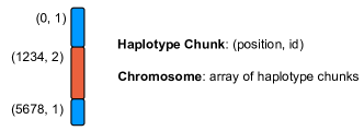
Figure 1: forqs chromosome representation. An individual chromosome is represented by a list of haplotype chunks. Each haplotype chunk is represented by two numbers (position, id): the position where it begins, and the identifier of the founding haplotype from which it is derived. This cartoon depicts a chromosome with 3 haplotype chunks as the result of recombination (double crossover) between two founder chromosomes.

forqs begins with a set of founding haplotypes representing the individuals in the initial generation. By assigning a unique identifier to each founding haplotype, individual haplotype chunks are tracked as they recombine over subsequent generations. For the purposes of simulation, any existing neutral variation on the haplotype chunks can be ignored. When simulating selection on standing variation, only those loci with fitness effects need to be tracked.

Internally, forqs represents an individual chromosome as a list of haplotype chunks (Figure 1). Individuals are diploid, and carry a user-specified number of chromosome pairs. To represent genetic variation at particular loci, forqs queries functions called VariantIndicators to obtain the variant values carried by the founding haplotypes at those loci.

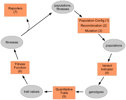
Figure 2: forqs modular design. The orange boxes represent places where the user can plug in configurable modules.

forqs uses configurable modules that are plugged into the main simulator to change the behavior of the simulation (Figure 2). forqs performs the following actions during a single cycle of the simulation:

• Generation of new populations: The PopulationConfigGenerator module (1) provides the simulator with a population configuration that specifies how to create individuals in the next generation from parents in the previous generation, based on user-specified population size and migration rate trajectories. Recombination and mutation are handled by a user-specified RecombinationPositionGenerator module (2) and/or MutationGenerator module (3), respectively.

• Genotyping: individuals are “genotyped” at a set of loci, using the VariantIndicator module to obtain variant (SNP) values for each individual. The list of loci to genotype is determined from the quantitative traits and reporters that are specified by the user.

• Quantitative trait evaluation: for each quantitative trait, a trait value is calculated for each individual, based on the individual’s genotype at loci affecting the trait. Each quantitative trait is specified by a QuantitativeTrait module.

• Fitness evaluation: the FitnessFunction module calculates each individual’s fitness based on the individual’s quantitative trait values.

• Reporting: each Reporter module updates its output files using current information from the populations (which includes genotypes, trait values, and fitnesses).

Each configurable module in Figure 2 is actually an interface with multiple implementations. The user specifies which module implementations to instantiate in a forqs configuration file. In addition to the primary modules shown in the diagram, there are several building block modules that provide basic functionality to the primary modules. For example, Trajectory modules provide a unified method for specifying values that change over time, such as population sizes or migration rates. Similarly, Distribution modules can be used to specify how to draw particular random values, for example, QTL positions or allele frequencies.

For example, to simulate populations undergoing neutral admixture, the user would specify a PopulationConfigGenerator module representing a stepping stone or island model with the desired population size and migration rate trajectories, and a RecombinationPositionGenerator with the desired recombination rate or map, but no quantitative traits. As another example, to simulate an artificial selection experiment with truncation selection on a single quantitative trait, the user would specify the quantitative trait loci (QTLs) and effect sizes, and choose a FitnessFunction module representing truncation selection with the desired proportion of individuals selected to produce the next generation. Alternatively, the user could indicate that the QTLs and effect sizes should be drawn randomly from user-specified distributions.

The representation of chromosomes as haplotype chunks in forqs makes very efficient use of memory, independent of the size of the chromosomes. However, memory usage grows linearly with the number of generations simulated, due to recombination. On a typical laptop computer, for a population size of 1 million, simulations take $\sim 1.5$ seconds per generation for neutral simulations and $\sim 3$ seconds per generation with quantitative traits and selection. Decreasing the population size allows the simulation of a greater number of generations in a reasonable amount of time: for a population size of 10000, it takes $\sim 3$ seconds per 100 generations (without selection, with a negligible increase with selection).

forqs has been extensively tested for correctness, both at the level of individual code units, and in its large-scale behavior in comparison to theoretical predictions from population genetics and quantitative genetics. Validation results, as well as tutorials and documentation can be found in the Supplementary Information.

About the image

The image on the first page was created based on haplotype frequency information reported during a forqs simulation. The image shows local haplotype frequencies (equivalently, local ancestry proportions) along a single chromosome. A single population was simulated with selection at two loci (one near each end of the chromosome). 25% of individuals (blue) in the initial generation carried the selected allele at the first locus, and a different 25% (green) carried the selected allele at the second locus. After 100 generations, the two selected variants have fixed in the population. All individuals carry one of the blue haplotypes in the region containing the first locus, as well as one of the green haplotypes in the region containing the second locus.

Contents

1. 1 Introduction
2. 2 Design and Implementation
3. 3 Getting Started
4. 4 Tutorial Introduction
   1. 4.1 A minimal example
   2. 4.2 Recombination and reporting output
   3. 4.3 Wright-Fisher simulation
   4. 4.4 Selection
   5. 4.5 Trajectories
   6. 4.6 Quantitative traits
   7. 4.7 Reporting haplotype frequencies
5. 5 Modules
   1. 5.1 Module types and interfaces
   2. 5.2 Module specification and instantiation
   3. 5.3 Top-level module: SimulatorConfig
      1. 5.3.1 Global simulation parameters
      2. 5.3.2 References to primary modules
   4. 5.4 Primary modules
      1. 5.4.1 PopulationConfigGenerator
      2. 5.4.2 MutationGenerator
      3. 5.4.3 RecombinationPositionGenerator
      4. 5.4.4 VariantIndicator
      5. 5.4.5 QuantitativeTrait
      6. 5.4.6 FitnessFunction
      7. 5.4.7 Reporter
   5. 5.5 Building block modules
      1. 5.5.1 Locus and LocusList
      2. 5.5.2 Trajectory
      3. 5.5.3 Distribution
6. 6 Simulating background variation
   1. 6.1 Example 1: No new mutations
   2. 6.2 Example 2: Including new mutations
7. 7 Validation
   1. 7.1 Single locus selection
   2. 7.2 Decay of linkage disequilibrium
   3. 7.3 Mutation-drift equilibrium
   4. 7.4 Response to selection
8. 8 Software development
   1. 8.1 Building the program
   2. 8.2 Structure of the codebase
   3. 8.3 Software architecture
      1. 8.3.1 Low-level data structures
      2. 8.3.2 Configurable modules
      3. 8.3.3 Mutation handling
   4. 8.4 Appendix: Boost libraries
   5. 8.5 Appendix: Cross-compilation targeting Windows

3 Getting Started

forqs binaries (Linux, OSX, and Windows) are distributed in zip file packages containing the executables, documentation, and example configuration files. The latest forqs packages are available here:
https://bitbucket.org/dkessner/forqs/downloads

forqs is a command line program that takes a single argument specifying the configuration file for the simulation:

    forqs config_file

The forqs packages include an examples directory containing several example configuration files. After unzipping the forqs package, you can run forqs directly from the package directory:

    bin/forqs examples/example_1_locus_selection.txt

forqs puts all output files in the output directory specified in the configuration file. After running this command, you will find a new directory output_example_1_locus_selection with the output from this simulation. For convenience, you can put the forqs executable somewhere in your PATH, e.g. ~/bin, so that you don’t have to type the path when running the program.

In addition to the document you are now reading, forqs packages include the forqs Module Reference (docs/forqs_module_reference.html, Figure 3), which contains details about each module, including parameter names, usage, and links to examples.

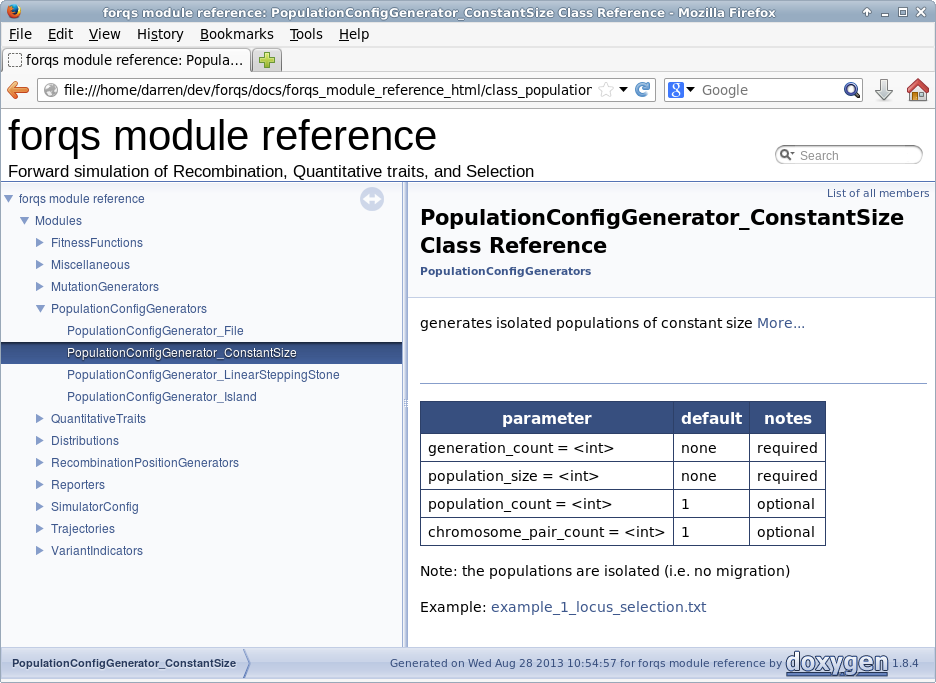
Figure 3: forqs Module Reference.

4 Tutorial Introduction

In this section we introduce forqs configuration files, starting with a minimal example and gradually adding modules to add complexity to the simulation. All example configuration files can be found in the examples directory of the forqs package.

4.1 A minimal example

We start with a minimal example configuration file:

#
# tutorial_0_minimal.txt
#

PopulationConfigGenerator_ConstantSize pcg
    population_size = 10
    generation_count = 3

SimulatorConfig
    output_directory = output_tutorial_0_minimal
    population_config_generator = pcg

There are two modules specified in this configuration file. The first module is PopulationConfigGenerator_ConstantSize, which we have assigned the object id pcg. The object id, which can be any text string, allows other objects to reference this object. We have set two parameters for this module, which specify the population size (population_size = 10) and the number of generations to simulate (generation_count = 3).

The second module is SimulatorConfig, the top-level module. This module must be specified last in the configuration file, because it has references to the primary modules (the general rule is: objects must be specified before they can be referenced by other objects). In this case, we are telling SimulatorConfig to use object pcg as our PopulationConfigGenerator, which is the only primary module that is required to be specified. The other primary modules have trivial defaults, and we leave them unspecified. In addition to the primary module references, SimulatorConfig also contains global simulation parameters. In this case, we have specified the output directory to be output_tutorial_0_minimal.

The simulator queries the PopulationConfigGenerator each generation to obtain a population configuration, which contains the information necessary to create the next generation from the previous one. In this case, the population configuration is the same each generation — it tells the simulator to create a population of 10 individuals with parents drawn from the same population in the previous generation.

When you run forqs on this example (tutorial_0_minimal.txt), you will see screen output showing that the simulation ran for 3 generations. You will also see the new output directory output_tutorial_0_minimal. If you look in this directory, you’ll see a single file: forqs.simconfig.txt. This file contains the configuration used for the simulation, including unspecified default parameters. However, there are no other output files in the directory, so we don’t actually know what happened during the simulation. To get more information, we need to specify Reporters to report output — we show how to do this in the next section.

4.2 Recombination and reporting output

In this example, we add modules to include recombination and report output:

#
# tutorial_1_recombination_reporter.txt
#

PopulationConfigGenerator_ConstantSize pcg
    generation_count = 3
    population_count = 1
    population_size = 10
    chromosome_lengths = 1e6

RecombinationPositionGenerator_Uniform rpg
    rate = 1

Reporter_Population reporter_population
    # update_step = 1

SimulatorConfig
    output_directory = output_tutorial_1_recombination_reporter
    population_config_generator = pcg
    recombination_position_generator = rpg
    reporter = reporter_population

When creating offspring chromosomes from parental chromosomes, the simulator uses the RecombinationPositionGenerator module to generate lists of recombination positions. In this case, we are using RecombinationPositionGenerator_Uniform, which chooses the positions uniformly at random along the chromosome. Note the use of the compound parameter chromosome_length_rate that specifies both the length of the chromosome and the recombination rate.

Reporter modules are used by forqs to output information about the simulation. The user can specify an arbitrary number of Reporters, depending on what output is desired. Reporter_Population outputs forqs population files, where each individual is represented as a list of chromosomes (one chromosome per line) and each chromosome is represented as a list of haplotype chunks. By default, population files will be produced only for the final generation — setting update_step = n will tell the Reporter_Population to output population files every n generations. You can see this by uncommenting (removing the ’#’ character) the update_step line in the configuration file and re-running the simulation.

The population files contain the raw information about the simulated individuals, and are not meant to be analyzed directly. Instead, they can be used to propagate existing neutral variation from the founding haplotypes of the initial generation to the mosaic haplotypes of the final generation (see Section 6).

However, we will use the population files to illustrate forqs’ internal representation of chromosomes. The first chromosome in the population file from the final generation is:

+ { (0,12) (704958,7) }

This means that the first chromosome of the first individual is made up of two haplotype chunks: the first chunk (0,12) starts at position 0 and comes from founder individual 12; the second chunk (704958,7) starts at position 704958 and comes from founder individual 7. Now comment out the following line in SimulatorConfig:

    recombination_position_generator = rpg

which ’un-plugs’ the RecombinationPositionGenerator from the simulator. Now re-run the simulation, specifying a different output directory on the command line:

    forqs tutorial_1_recombination_reporter.txt output_directory=out2

When you look at the resulting final population file, you will see that all chromosomes consist of a single chunk, as you would expect with no recombination.

4.3 Wright-Fisher simulation

Our next example is a simple Wright-Fisher simulation where we track the allele frequency at a single locus under neutral drift:

#
# tutorial_2_wright_fisher.txt
#

PopulationConfigGenerator_ConstantSize pcg
    population_size = 100
    generation_count = 200
    # population_count = 10

Locus my_locus
    chromosome = 1
    position = 100000

VariantIndicator_SingleLocusHardyWeinberg vi
    locus = my_locus
    allele_frequency = .5

Reporter_AlleleFrequencies reporter_allele_freqs
    locus = my_locus

SimulatorConfig
    output_directory = output_tutorial_2_wright_fisher
    population_config_generator = pcg
    variant_indicator = vi
    reporter = reporter_allele_freqs

In this example, the population size is 100, the initial allele frequency is .5, and the simulation runs for 200 generations.

The Locus module defines a single site — in this case it is position 100000 on chromosome 1. The Locus has id my_locus, and this id is used by two other modules to refer to this locus.

As we saw in the previous example, forqs represents chromosomes as lists of haplotype chunks, with no information about nucleotides or variant (SNP) values at any position. (To be concrete, we think of a variant value as being 0 or 1, but forqs variant values can be anything in the range 0–255, so we are not restricted to bi-allelic SNPs). However, if we give forqs the variant values for the founding haplotypes, it can calculate variant values for any mosaic chromosome. This information is represented by a VariantIndicator, which is a function that tells forqs which founding chromosomes contain which variants.

In our case, we specify a VariantIndicator_SingleLocusHardyWeinberg, which assigns variants to individuals in Hardy-Weinberg proportions. Because we have specified an initial allele frequency of .5, this means that of the founding individuals, 25% will be homozygote 0, 25% will be homozygote 1, and 50% will be heterozygotes.

We also want to track the allele frequency at this locus, so we specify a Reporter_AlleleFrequencies, which reports the allele frequency at each generation. You will find the output in the file allele_frequencies_chr1_pos100000.txt.

You may have noticed the commented line with the parameter population_count = 10. By uncommenting this line, you will tell forqs to simulate 10 populations. PopulationConfigGenerator_ConstantSize does not allow migration between populations, so this effectively gives 10 independent Wright-Fisher simulations. The resulting allele frequency trajectories can all be found in the same output file, with one column per population. As expected, you will see that the alternate allele (1) has been fixed or lost in some populations, and is still polymorphic in others.

4.4 Selection

In this example, we add selection to our Wright-Fisher simulation.

#
# tutorial_3_selection.txt
#

PopulationConfigGenerator_ConstantSize pcg
    population_size = 100
    generation_count = 100
    population_count = 10

Locus my_locus
    chromosome = 1
    position = 100000

VariantIndicator_SingleLocusHardyWeinberg vi
    locus = my_locus
    allele_frequency = .5

QuantitativeTrait_SingleLocusFitness qt
    locus = my_locus
    w0 = 1
    w1 = 1.1
    w2 = 1.2

FitnessFunction_Identity ff
    quantitative_trait = qt

Reporter_AlleleFrequencies reporter_allele_freqs
    locus = my_locus

Reporter_MeanFitnesses reporter_mean_fitnesses

Reporter_DeterministicTrajectories reporter_deterministic_trajectories
    initial_allele_frequency = .5
    w0 = 1
    w1 = 1.1
    w2 = 1.2

SimulatorConfig
    output_directory = output_tutorial_3_selection
    population_config_generator = pcg
    variant_indicator = vi
    quantitative_trait = qt
    fitness_function = ff
    reporter = reporter_allele_freqs
    reporter = reporter_mean_fitnesses
    reporter = reporter_deterministic_trajectories

For this simulation, we add a quantitative trait that is determined by the genotype at a single locus. In fact, in our case, the quantitative trait is fitness (QuantitativeTrait_SingleLocusFitness), and we use the identity function for our fitness function (FitnessFunction_Identity). The parameters w0, w1, w2 are used to specify the fitness for individuals with genotype 0, 1, and 2, respectively. In general, a quantitative trait can depend on multiple loci on multiple chromosomes, and fitness can depend on multiple quantitative traits.

We also add some useful Reporters that output the mean fitnesses of the populations as well as the deterministic trajectories expected in the limit of infinite population size. These output files can be easily read into a plotting application (e.g. R) to compare the random trajectories with the deterministic trajectories (Figure 4).

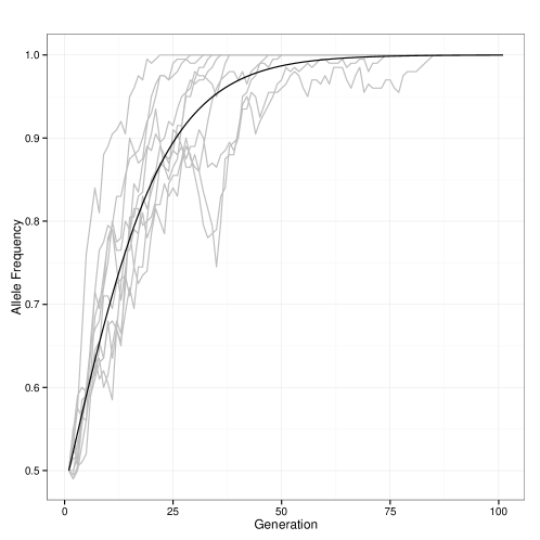
Figure 4: Allele frequency trajectories from selection simulation.

4.5 Trajectories

This section shows how to use Trajectory modules to specify population sizes that change over time. In general, Trajectory modules can be used to specify any numeric value that varies by population and generation – other examples include mutation rates and migration rates.

In the first example (tutorial_4a_trajectories.txt), there are two populations following the same population size trajectory: constant size 100 until generation 2, followed by a linear increase in population size until it reaches 400 at generation 5, after which the population size stays at 400. This is accomplished by specifying each piece (Trajectory_Constant, Trajectory_Linear, Trajectory_Constant) and composing the pieces together with Trajectory_GenerationComposite.

#
# tutorial_4a_trajectories.txt
#

Trajectory_Constant popsize_1
    value = 100

Trajectory_Linear popsize_2
    begin:value = 2 100
    end:value = 5 400

Trajectory_Constant popsize_3
    value = 400

Trajectory_GenerationComposite popsize
    generation:trajectory = 0 popsize_1
    generation:trajectory = 2 popsize_2
    generation:trajectory = 5 popsize_3

PopulationConfigGenerator_LinearSteppingStone pcg
    generation_count = 8
    population_count = 2
    population_size = popsize

SimulatorConfig
    output_directory = output_tutorial_4a_trajectories
    write_popconfig = 1        # set this flag to write out the popconfig file
    population_config_generator = pcg

Note that PopulationConfigGenerator_LinearSteppingStone has a population_size parameter whose value must be the id of a Trajectory module (rather than a numeric value). Also, unless otherwise specified, each Trajectory gives the same numeric value for each population in a given generation. You can see the raw population configuration generated by including the parameter write_popconfig = 1, which tells forqs to write out the population configs in a file forqs.popconfig.txt. After running this example, you can examine forqs.popconfig.txt to see the population sizes.

In the next example (tutorial_4b_trajectories.txt), population 1 follows the same population size trajectory as in the first example, while population 2 experiences exponential growth, doubling each generation (with initial population size 1000). In order to specify this scenario, each population size trajectory is specified separately (popsize_pop1 and popsize_pop2 in this example), and the two are composed with Trajectory_PopulationComposite. When Trajectory_PopulationComposite is queried for a value for a population, it returns the value obtained from the appropriate sub-trajectory.

#
# tutorial_4b_trajectories.txt
#

# population 1

Trajectory_Constant popsize_pop1_1
    value = 100

Trajectory_Linear popsize_pop1_2
    begin:value = 2 100
    end:value = 5 400

Trajectory_Constant popsize_pop1_3
    value = 400

Trajectory_GenerationComposite popsize_pop1
    generation:trajectory = 0 popsize_pop1_1
    generation:trajectory = 2 popsize_pop1_2
    generation:trajectory = 5 popsize_pop1_3

# population 2

Trajectory_Exponential popsize_pop2
    generation_begin = 0
    value_begin = 1000
    rate = 0.693147     # log(2); population size doubles each generation

# composite trajectory

Trajectory_PopulationComposite popsize
    trajectories = popsize_pop1 popsize_pop2

PopulationConfigGenerator_LinearSteppingStone pcg
    generation_count = 8
    population_count = 2
    population_size = popsize

SimulatorConfig
    output_directory = output_tutorial_4b_trajectories
    write_popconfig = 1        # set this flag to write out the popconfig file
    population_config_generator = pcg

4.6 Quantitative traits

In this section, we present an example of specifying a quantitative trait by specifying quantitative trait loci (QTLs) and their effect sizes.

#
# tutorial_5_qtl.txt
#

PopulationConfigGenerator_ConstantSize pcg
    generation_count = 10
    population_count = 1
    population_size = 100
    chromosome_pair_count = 3
    chromosome_lengths = 1e6 1e6 1e6

Locus locus1
    chromosome = 1
    position = 1000

Locus locus2
    chromosome = 2
    position = 2000

Locus locus3
    chromosome = 3
    position = 3000

LocusList loci
    loci = locus1 locus2 locus3

VariantIndicator_Random vi
    locus_list:population:frequencies = loci * .5 .5 .5

QuantitativeTrait_IndependentLoci qt
    qtl = locus1 0 .1 .2
    qtl = locus2 0 .2 .4
    qtl = locus3 0 .1 .2
    environmental_variance = .05

FitnessFunction_TruncationSelection ff
    quantitative_trait = qt
    proportion_selected = .5

Reporter_AlleleFrequencies reporter_allele_frequencies
    quantitative_trait = qt

Reporter_TraitValues reporter_trait_values
    quantitative_trait = qt
    write_full = 1

SimulatorConfig
    output_directory = output_tutorial_5_qtl
    population_config_generator = pcg
    variant_indicator = vi
    quantitative_trait = qt
    fitness_function = ff
    reporter = reporter_allele_frequencies
    reporter = reporter_trait_values
    write_vi = 1

In this example, we specify a single population (size 100) where individuals have 3 chromosomes. We specify 3 loci, each on a different chromosome.

VariantIndicator_Random is used to assign variants to the initial haplotypes randomly, according to the specified allele frequencies – in this case, the variant allele frequency is .5 for each locus. The ’*’ indicates that all populations have the same allele frequencies – because there is only one population, we could have used ’1’ in place of ’*’. The parameter write_vi = 1 in SimulatorConfig tells forqs to write the file forqs.vi.txt containing lists of the initial haplotypes carrying the variant allele at each locus.

QuantitativeTrait_IndependentLoci specifies a quantitative trait where the effects of variants at different loci are independent of each other, i.e. there are no epistatic effects. Each QTL is listed with its per-genotype effects – in this case, individuals with genotype 0, 1, or 2 at locus1 will have 0, .1, or .2 added to their trait value, respectively. Alternatively, QTL effect sizes and dominance values can be chosen randomly according to specified distributions. For an example of this, see example_qtl_random.txt which also demonstrates the use of LocusList_Random to pick the loci randomly as well.

In this example, FitnessFunction_TruncationSelection assigns fitness values of 1 to individuals in the upper half of the distribution, and 0 to individuals in the lower half (proportion_selected = .5). Reporter_AlleleFrequencies uses the parameter quantitative_trait = qt, which tells it to report allele frequencies for all QTLs associated with the trait. Reporter_TraitValues reports mean trait values for the population each generation; the parameter write_full = 1 tells it to also report individual trait values for each generation.

4.7 Reporting haplotype frequencies

This example shows the use of Reporter_HaplotypeFrequencies to report local haplotype frequencies in the simulated populations.

In this example, there is a single locus that confers an additive fitness advantage to the individuals carrying the selected variant. The VariantIndicator specifies which haplotype ids actually carry the variant: in this case, VariantIndicator_IDRange assigns the value 1 to the first 1000 haplotype ids, i.e. the first 500 individuals are homozygous for the selected variant.

Reporter_HaplotypeFrequencies uses a HaplotypeGrouping module that specifies how haplotype ids should be grouped. The grouping can be as fine-grained as a single haplotype id per group, but for simplicity we have specified just two groups: those individuals who carry the selected variant, and those who don’t. Reporter_HaplotypeFrequencies then reports local proportions of the two groups in the population.

We have specified a relatively high recombination rate (3 crossovers per meiosis on average) and strong selection (.1 selection coefficient) in order to illustrate the change in local haplotype frequencies in just a few generations. After running the example, the output file haplotype_frequencies_chr1_final_pop1.txt shows that haplotypes carrying the selected variant have risen to high frequency near the selected locus, but not as much in regions farther away, due to recombination. The parameter update_step = k will result in reporting of local haplotype frequencies every k generations (default is to report only the final generation).

#
# tutorial_6_haplotype_frequencies.txt
#

PopulationConfigGenerator_ConstantSize pcg
    generation_count = 20
    population_count = 1
    chromosome_pair_count = 1
    chromosome_lengths = 1e6
    population_size = 1000

RecombinationPositionGenerator_Uniform rpg
    rate = 3

Locus selected_locus
    chromosome = 1
    position = 500000

VariantIndicator_IDRange vi
    locus:start:count:step:value = selected_locus 0 1000 1 1

QuantitativeTrait_IndependentLoci qt
    qtl = selected_locus 1 1.1 1.2

FitnessFunction_Identity ff
    quantitative_trait = qt

Reporter_AlleleFrequencies reporter_allele_frequencies
    quantitative_trait = qt

HaplotypeGrouping_Uniform hg
    ids_per_group = 1000        # 2 groups of 500 individuals

Reporter_HaplotypeFrequencies reporter_haplotype_frequencies
    haplotype_grouping = hg
    chromosome_step = 1e5
    #update_step = 1

SimulatorConfig
    output_directory = output_tutorial_6_haplotype_frequencies
    population_config_generator = pcg
    recombination_position_generator = rpg
    variant_indicator = vi
    quantitative_trait = qt
    fitness_function = ff
    reporter = reporter_allele_frequencies
    reporter = reporter_haplotype_frequencies

5 Modules

In this section, we give an overview of forqs modules. For information about specific forqs modules, including parameter names, usage, and links to examples, please refer to the forqs Module Reference (forqs_module_reference.html).

5.1 Module types and interfaces

forqs has a single top-level module called SimulatorConfig. There are seven primary modules, corresponding to the orange boxes Figure 2, which represent the main places where forqs can be customized. There are also several building block modules, which are used by the primary modules.

Multiple modules may share a common interface, as indicated by their names. For example, Reporter_Timer and Reporter_AlleleFrequencies both implement the Reporter interface. Modules with the same interface can be used interchangeably by the simulator.

In addition, specific modules can be instantiated multiple times (with different object ids and parameters) – for example, Reporter_AlleleFrequencies can be used to report allele frequencies at several different loci.

By mixing and matching different modules, the user has a great deal of flexibility in creating customized simulation scenarios. In addition, forqs can easily be extended with new functionality by adding new modules that implement existing module interfaces.

5.2 Module specification and instantiation

Each forqs module specified in the configuration file corresponds to an object that is instantiated by the simulator before the simulation starts. The first line of a module specification contains the module name and object id. Each subsequent line specifies a parameter of the module, formatted as a name-value pair: name = value. The value is read as a string, but may be interpreted as an integer, floating point, string, or list, depending on the parameter. Each module determines how its parameter values are interpreted, and interpretation errors are reported to the user. In some modules, multiple parameter values may be specified with the same name, in which case each value specified is appended to a list. A blank line ends the specification for that module.

As an example, here is the specification of a Locus module, which represents a single nucleotide position:

Locus my_locus
    chromosome = 1
    position = 500000

The first line specifies a Locus object with id my_locus. The two parameters specify which chromosome (1) and the position on the chromosome (500000).

After parsing this module specification, the simulator instantiates a Locus object, and puts the object in a registry under the name my_locus. Subsequently instantiated objects may need a reference to this object, which can be obtained by looking up the object by name in the registry. Because modules are instantiated in the order they are specified in the configuration file, it is important to specify an object before it is referenced by other objects (otherwise forqs will produce an error message that it couldn’t find the referenced object in the registry).

Object references are specified as string-valued parameters, where the value contains the object id of the referenced object. For example, the following is the specification of a Reporter module that holds a reference to our example Locus object my_locus:

Reporter_AlleleFrequencies reporter_allele_frequencies
    locus = my_locus

One final note on a parameter naming convention used in forqs – for parameters where the value is a list of sub-parameters, the parameter name should be a concatenation of the sub-parameters. This convention allows easier reading and editing of configuration files without the need to consult documentation. For example, Trajectory_GenerationComposite represents a list of Trajectory modules, to be followed piecewise at specified generations. This module is parametrized by a list of pairs (generation, trajectory), using the parameter name generation_trajectory:

Trajectory_GenerationComposite id_migration_rate
    generation_trajectory = 0 id_migration_rate_0
    generation_trajectory = 5 id_migration_rate_1

In this case, the module configuration can be interpreted as follows: at generation 0 use trajectory id_migration_rate_0, and then at generation 5 start using trajectory id_migration_rate_1.

5.3 Top-level module: SimulatorConfig

SimulatorConfig is the top-level module containing:

• global simulation parameters

• references to the primary modules

Because SimulatorConfig has references to the primary modules, it must be specified last in the configuration file.

5.3.1 Global simulation parameters

The main global simulation parameters are:

• output_directory: forqs will create this directory and place all output files here

• seed: seed for the random number generator

Command line parameters can also be specified on the command line as name=value with no whitespace, as shown in this example:

    forqs config.txt output_directory=mydir seed=12345

If a parameter is specified on both the command line and in the configuration file, the command line takes precedence.

If no random seed is specified, forqs will first look in the current working directory for the file forqs.seed containing a previously generated seed. If no seed is found, forqs will generate a new seed from the system time. At the end of each run, forqs generates a random seed and writes it to forqs.seed. To summarize, forqs looks for the seed in the following places, in order of preference:

1. command line

2. configuration file

3. forqs.seed

4. system time

5.3.2 References to primary modules

Of the primary modules, only PopulationConfigGenerator is required to be specified, because it contains necessary information about population sizes and the number of generations. The rest of the modules default to trivial implementations. The primary modules specified in SimulatorConfig are:

1. PopulationConfigGenerator

   • required – no default

2. RecombinationPositionGenerator

   • default: RecombinationPositionGenerator_Trivial (no recombination – whole chromosomes are transmitted, chromosome pairs segregate independently)

3. MutationGenerator

   • default: none (no mutation)

4. VariantIndicator

   • default: VariantIndicator_Trivial (always returns 0)

5. QuantitativeTrait

   • default: none (no quantitative traits)

   • multiple QuantitativeTraits may be defined

6. FitnessFunction

   • default: FitnessFunction_Trivial (always returns 1 – all individuals have equal fitness)

7. Reporter

   • default: none (no reporters)

   • multiple Reporters may be defined

5.4 Primary modules

5.4.1 PopulationConfigGenerator

For the reproduction/transmission step, in addition to information about the current populations, the simulator needs to know the population configuration for the next generation, which includes:

• number and sizes of the populations in the next generation

• mating distribution, which describes how parents are chosen from the current generation to create offspring in the next generation

The PopulationConfigGenerator module provides an interface for the simulator to obtain a population configuration for each generation.

For the initial generation, individuals are assigned haplotype ids sequentially starting at 0, with two ids assigned per individual (one for the maternal chromosomes, and one for the paternal chromosomes). Id offsets can be used to make it easier to distinguish between populations – for example, individuals from population 1 may be assigned ids starting at 0, and individuals from population 2 may be assigned ids starting at 1000000.

PopulationConfigGenerator_File allows specification of a population configuration for each generation, giving the user precise control over the demographic histories of the simulated populations.

Alternatively, forqs provides higher level PopulationConfigGenerators that allow the user to specify time-dependent population size and migration rate trajectories (e.g. PopulationConfigGenerator_LinearSteppingStone). When a migration rate is specified from a source population to a destination population, it is interpreted to be the probability that a new child in the destination population has parents in the source population. Equivalently, it is the expected proportion of individuals in the next generation of the destination population whose parents were in the source population.

For debugging purposes, forqs optionally outputs the file forqs.popconfig.txt with the population configuration that was used for each generation during the simulation. This option can be selected by setting the write_popconfig parameter in SimulatorConfig:

    write_popconfig = 1

5.4.2 MutationGenerator

The user may specify a MutationGenerator module to generate random mutations during the simulation. MutationGenerator provides a single interface through which the simulator obtains a list of new mutations for a particular generation. However, MutationGenerator implementations may differ in how they generate this list of mutations. For example, MutationGenerator_SingleLocus generates mutations only at a single site, while MutationGenerator_Regions generates mutations in multiple regions with different (possibly time-dependent) mutation rates. In any case, the user will most likely want to also specify Reporter_Regions to report the final mutated sequences at the end of the simulation.

forqs current mutation implementation creates a new haplotype id for each new mutation, storing it in a haplotype ancestry tree (so that information about the ancestral haplotype can be preserved). This results in memory usage that increases with each generation, which may cause performance degradation in simulations involving a high total mutation rate for a large number of generations. (Here total mutation rate means $\theta L$, where $\theta=4N\mu$ is the population-scaled per-site mutation rate and $L$ is the total length of the genomic region where new mutations are being generated).

5.4.3 RecombinationPositionGenerator

The RecombinationPositionGenerator module provides an interface for the simulator to obtain a list of recombination positions – the position list is used to create an offspring chromosome from a pair of parental chromosomes.

RecombinationPositionGenerator_RecombinationMap generates recombination positions according to previously estimated recombination maps (e.g. from HapMap project).

5.4.4 VariantIndicator

Internally, forqs represents each individual chromosome as a list of haplotype chunk ids, with no information about particular variants (e.g. SNP 0/1 values) carried on that chromosome. In order to obtain an individual’s genotype at a locus, the simulator must use a VariantIndicator, which is essentially a function that maps:

$$(\emph{locus},\emph{haplotype id})\mapsto\emph{variant value}$$

In general, a VariantIndicator needs to specify variant values only at selected loci, because neutral loci have no effect on the simulation. Ancestral neutral variation that is present on the haplotypes of the founders (individuals in the initial generation) can be propagated to individuals at the end of the simulation using the forqs_map_ms tool included in the forqs package.

5.4.5 QuantitativeTrait

A QuantitativeTrait module represents a single quantitative trait. The module encapsulates the information needed to calculate the trait value for each individual based on the individual’s genotypes at a list of user-specified loci. For example, QuantitativeTrait_IndependentLoci allows the user to specify loci and effect sizes, and the trait value for each individual is calculated by combining that individual’s locus-specific effects additively (with user-specified environmental variance).

5.4.6 FitnessFunction

A FitnessFunction module represents the function used to calculate an individual’s fitness based on the individual’s trait values. In simple cases, the quantitative trait may actually be fitness, in which case the user may simply use FitnessFunction_Identity. In more complicated cases, fitness may depend non-trivially on one or more quantitative traits.

5.4.7 Reporter

Reporter modules are used to report information during the simulation. For example, Reporter_AlleleFrequencies reports the allele frequency of a user-specified locus at each generation. The full list of available Reporters can be found in the forqs Module Reference.

5.5 Building block modules

5.5.1 Locus and LocusList

The Locus module represents a single site on a chromosome, specified by the chromosome pair index and position on the chromosome:

Locus my_locus
    chromosome_pair_index = 0
    position = 500000

Note that the chromosome pairs use 0-based indexing, so chromosome_pair_index = 0 refers to the first chromosome pair.

LocusList modules are used to define a list of loci. The list can be specified in two ways – in the first, loci are specified by chromosome number and position:

LocusList locus_list
    chromosome:position = 1 1000123
    chromosome:position = 2 2000234
    [...]

Alternatively, the loci can be references to previously specified Locus objects:

LocusList locus_list_2
    loci = my_locus_1 my_locus_2 [...]

Also, a random list of loci can be generated with LocusList_Random:

LocusList_Random locus_list_random
    locus_count = 10

5.5.2 Trajectory

In simple situations, constant parameter values can be used to specify an aspect of the simulation. For example, it is common in population genetics to simulate models where population sizes are constant. In more complicated scenarios, parameter values (e.g. population sizes, migration rates, mutation rates, optimal quantitative trait values) may vary in space (population) or in time (generation).

forqs uses Trajectory modules to describe such varying quantities. In essence, a Trajectory represents a function:

$$(\emph{population index},\emph{generation index})\mapsto\emph{value}$$

Trajectories can be built by the user by starting with simple building blocks (e.g. constant, linear, polynomial, exponential functions) and then composed either by population or by generation. Once the Trajectory has been defined, it can be referenced by name to be used as the parameter of another module. Note that if a module expects a particular parameter to be a Trajectory, it is an error to pass a constant integer or floating point number as the parameter value. In this case, if the user really wants a constant parameter value, Trajectory_Constant should be specified.

5.5.3 Distribution

Distribution modules represent probability distributions. These modules are used to model, for example, effect sizes for QTLs or environmental variance for a quantitative trait.

Distribution_Constant can be used in situations where a module requires a reference to a Distribution but a constant value is desired.

6 Simulating background variation

Forward-in-time simulators often use a burn-in period to allow neutral variation to reach mutation-drift equilibrium. An alternative strategy, adopted by forqs, is to use an existing program (such as Dick Hudson’s ms) to generate neutral variation for the founders in the initial population. Chromosomes in the final populations are mosaics of the founder chromosomes, so neutral variation can be propagated to the mosaic chromosomes to generate sequence (or SNP) data. The tool forqs_map_ms is included in forqs packages for this purpose. In this section we discuss the propagation procedure using two examples.

6.1 Example 1: No new mutations

The first example is a simple case where there are no new mutations introduced during the forqs simulation. This case includes many scenarios of interest where the variation in the population has been generated over a small number of generations, primarily by recombination and recent admixture between historically isolated (or inbred) populations.

In this case, the propagation of neutral variation is straight-forward: sequence variants on founder haplotypes are mapped onto the mosaic chromosomes of the final population. However, there are many details about the mapping that must be specified by the user in a mapping configuration file. forqs produces final populations of individuals that may carry multiple pairs of chromosomes, with absolute positions specified by integers. ms outputs single chromosomes, with relative positions specified by floating point numbers. The mapping configuration thus needs to specify an integer range of positions on a particular chromosome that correspond to the ms relative positions in the range [0,1]. In addition, the user must specify how forqs haplotype ids correspond to the ms-format variant sequences.

In the examples directory, the following 4 files can be found:

• population_example.txt (forqs population data)

• ms_test_data_1.txt, ms_test_data_2.txt (ms-format files)

• ms_map_config.txt (mapping configuration file)

Perform the mapping using the following command:

forqs_map_ms population_example.txt ms_map_config.txt > output.ms

The resulting sequences in output.ms are mosaics of the sequences in the input ms-format files. For example, the first chromosome of the first individual is a mosaic of haplotypes 0, 1, 2, and 3, corresponding to the sequences ’aaaaaaaaa’, ’bbbbbbbbb’, ’ccccccccc’, and ’ddddddddd’, respectively. The output sequence for this chromosome is ’aabccccdd’. Note that alphabetic letters are used in these example sequences for illustration only – real ms output consists of 0’s and 1’s.

6.2 Example 2: Including new mutations

In scenarios where it is important to include new mutations in addition to ancestral neutral variation, the mapping procedure has one additional complication. When simulating forward in time, the neutral variants carried by individuals have no effect on the dynamics of the simulation. forqs takes advantage of this by ignoring (i.e. not storing in memory) any ancestral neutral variation on the founding haplotypes. Each new mutation generated in forqs results in a new haplotype id. Because of this, it is necessary to use an id ancestry map to translate the new ids back to the ancestral ids before performing the mapping. After the neutral variation has been mapped, the new mutations can then be merged with the ancestral variants. This procedure is detailed in the following shell script (and data files referenced in the script), which runs a complete example of a forqs simulation followed by mapping ms sequences (with new mutations merged):

    examples/ms_map_example_new_mutations.sh

7 Validation

forqs has an extensive set of unit tests that verify the correctness of individual code modules. In addition, in order to validate the larger-scale behavior of the simulations, we have compared forqs simulation results to theoretical predictions from population genetics and quantitative genetics.

7.1 Single locus selection

We first considered simple scenarios where an individual’s fitness is determined by that individual’s genotype at a single locus, under a wide range of fitness effect sizes and dominance values. We compared the simulated allele frequency trajectories to the deterministic trajectories predicted in the limit of infinite population size.

In all cases, the simulated trajectories closely followed the deterministic trajectories, with better agreement in simulations with larger population sizes, as expected. Figure 5 shows the case of additive positive selection, for population sizes of 100 and 1000.

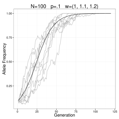
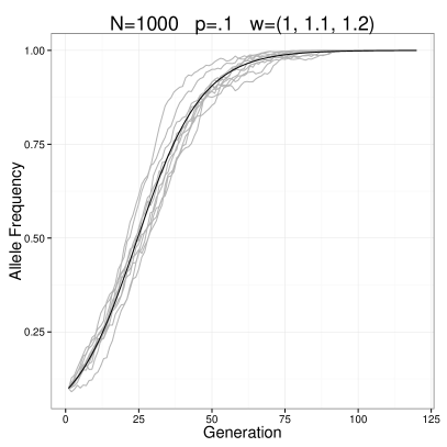
Figure 5: Selection on a single locus. The dark curves show the deterministic trajectories, and the lighter curves show simulated trajectories. Populations of size 100 and 1000 were simulated with additive fitness effect .1 at a single locus, with the selected variant having initial allele frequency .1.

7.2 Decay of linkage disequilibrium

In the limit of infinite population size, linkage disequilibrium (measured by $D$, the correlation between two variants at different sites) decays geometrically at rate $1-r$, where $r$ is the recombination rate (see Figure 6 for an example run).

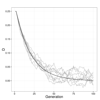
Figure 6: Decay of linkage disequilibrium. The dark curve shows the deterministic trajectory, and the lighter curves show simulated trajectories. In this example, $D=.25$ initially and $r=.05$.

7.3 Mutation-drift equilibrium

To validate our mutation implementation, we approximated the infinite-sites model by simulating mutations generated randomly in large regions (1mb). We set the per-site mutation rate to make the population-scaled mutation rate $\theta=10$, and simulated for enough generations to reach mutation-drift equilibrium.

We then compared the resulting site-frequency spectra $\{\xi_{i}\}$ to theoretical predictions, where $\xi_{1}$ is the number of singletons, $\xi_{2}$ is the number of doubletons, etc. in the sample. Coalescent theory predicts that $\xi_{i}=\theta/i$ in expectation (Fu 1995), under the assumption that the sample size is small compared to the population size. When the sample size is close to the population size, the Wright-Fisher model is expected to have approximately 12% more singletons and 2% less doubletons compared to the coalescent expected values (Wakeley and Takahashi 2003).

Site frequency spectra generated from the full population agree with the Wright-Fisher large sample expected values, and site frequency spectra from smaller samples agree with the coalescent expected values, as expected (Figure 7).

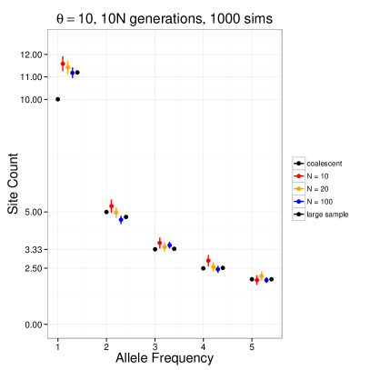
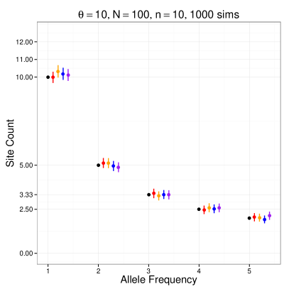
Figure 7: Mutation-drift equilibrium. (left) Simulations for different population sizes are shown, together with expected values for both the coalescent and Wright-Fisher with large sample size. (right) Small samples taken from a larger simulated population agree with the coalescent expected values.

7.4 Response to selection

To validate our implementation of selection on quantitative traits, we simulated a quantitative trait with 10 QTLs with identical additive effect sizes and initial allele frequencies, which gives an approximately normal distribution of trait values in the population. We also used the forqs fitness function FitnessFunction_TruncationSelection, which selects a specified proportion of individuals at the upper tail of the trait value distribution to produce offspring for the next generation.

The Breeder’s Equation from quantitative genetics (Gillespie 2004; Falconer and Mackay 1996) predicts the response to selection $R$ from the heritability of the trait $h^{2}$ and the selection differential $S$:

$$R =h^{2}S$$

where the $S$ and $R$ are the selected parent mean and offspring mean, respectively, measured as deviations from the population mean.

Simulations run with various values for the heritability and proportion of individuals selected agree with the response values predicted from the Breeder’s Equation (Figure 8).

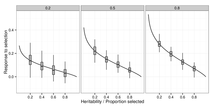
Figure 8: Response to selection 3 panels show simulations run at different heritability levels (.2, .5, .8), with varying proportions of selected individuals (.2, .4, .6, .8) (100 simulations each). The dark curves show the response values predicted from the Breeder’s Equation.

8 Software development

8.1 Building the program

forqs is written in C++, and makes extensive use of the Boost libraries, including the Boost build system. It is regularly built and tested on OSX and Linux. In addition, Windows binaries are built using cross-compilation with gcc on Linux.

The code can be obtained via git from bitbucket:

    git clone https://bitbucket.org/dkessner/forqs.git

If you have the both the Boost libraries and the Boost build system installed, you can build forqs with the bjam tool, which is the Boost build system’s equivalent of make:

    cd forqs/src
    bjam

8.2 Structure of the codebase

Most code units in the forqs project consist of three files:

• interface (header file)

• implementation (cpp file)

• unit test (cpp file)

For example, the code for the Locus module can be found in the files Locus.hpp, Locus.cpp, LocusTest.cpp.

The unit test for each code unit is run during the build; the build is successful only if all unit tests pass.

In addition to the unit tests, there are also regression tests, consisting of scripts in the regression_test directory. These tests prevent unintended behavior changes in the software during new development. Most of the tests are based on the example configuration files in the examples directory, and consist of running forqs and performing a diff comparison with known output. The regression tests are controlled by a Makefile, and run by make.

The codebase includes all documentation, including the Latex source code for this document. The forqs Module Reference is generated by Doxygen from the source code – each module is documented using Doxygen markup in the module’s header file, immediately preceding the module’s class declaration.

8.3 Software architecture

This section describes some of the design details of forqs that may be of interest to programmers who would like to add new features.

8.3.1 Low-level data structures

These are the basic low-level data structures used by forqs:

• HaplotypeChunk: a pair of integers (position, id)

• Chromosome: an array of HaplotypeChunks

• Organism: an array of pairs of Chromosomes

• Population: an array Organisms

In this setup, Population can be seen as an array of arrays, which requires a significant number of memory allocations. To avoid these memory allocations, Population was re-implemented as a two dimensional array of Chromosome pairs, resulting in a roughly 30% speedup.

The implementations produce identical results, and can be used interchangeably. To accomplish this, Population is actually an interface class, with two concrete implementations: Population_Organisms and Population_ChromosomePairs. While the latter is faster, the former can be more convenient for testing purposes.

In order to handle both cases in a unified manner, the class ChromosomePairRange represents the begin/end of chromosome pairs belonging to a single individual, and ChromosomePairRangeIterator does the appropriate iteration through individuals, depending on the memory layout of the population.

8.3.2 Configurable modules

Configurable modules in forqs are represented by the Configurable abstract base class, which defines the common interface through which objects are instantiated and initialized based on parameters specified by the user. The top-level module (SimulatorConfig), all primary modules (e.g. PopulationConfigGenerator, Reporter, etc.), and all building block modules (e.g. Trajectory, Locus) implement the Configurable interface.

The Configurable interface describes the functionality required to serialize an object’s configuration, which must be representable as a list of name-value pairs. (This is not actually very restrictive, since the value can be anything representable as a string, including an array of numbers).

Configurable objects are instantiated by SimulationBuilder_Generic, which handles the mapping from the module name to the actual C++ class. Each object in the user-specified configuration file is instantiated and registered by name so that other objects can obtain references to it if necessary. SimulationBuilder_Generic produces the final SimulatorConfig used by forqs for the simulation. (Note on the name: there were other SimulationBuilder classes that constructed SimulatorConfigs based on a more limited set of parameters – these have since been deprecated in favor of the more generic specification via configuration files.)

After instantiation, Configurable objects are configured/initialized in two steps. First, the configure() method sets any parameters specific to this module that are specified by the user. Second, after all objects have been configured, the initialize() method allows the modules to communicate with each other. For example, objects that need information about the lengths of the chromosomes (e.g. for recombination) can query the PopulationConfigGenerator, which has this information.

Configurable objects are instantiated, configured, and initialized in the order they are specified in the configuration file. It is important to note that while objects can obtain references to previously instantiated objects during the configure() step, they should not try to communicate via these references until the initialize() step, since the objects they refer to may not be fully initialized until then.

The main Simulator object interacts with Configurable objects through intermediate interfaces. This allows the main simulation logic to be separated from the specific behavior implemented by the various Configurable modules. For example, Reporter_AlleleFrequencies and Reporter_TraitValues both implement the Reporter interface. Simulator will give each Reporter information about the current populations, but doesn’t need to know what they do with this information. As another example, the Simulator gives a QuantitativeTrait object information about individuals’ genotypes and expects to receive trait values for each individual, but doesn’t need to know details about how this is accomplished.

The Configurable interface also facilitates some features that make forqs more user-friendly, because it provides a translation layer between the user and program internals. For example, while 0-based indexing is used internally, from the user’s perspective chromosomes and populations are numbered starting with 1. Also, Configurable modules can support multiple alternate parametrizations. For example, linear trajectories may be parametrized by slope-intercept or by two endpoints, and exponential distributions may be specified by the mean or the rate, depending on which is more natural for a particular scenario.

8.3.3 Mutation handling

Because forqs tracks haplotype chunks rather than sequences of variants, mutation is necessarily more complicated than recombination. This is because a new point mutation essentially creates a new haplotype that is identical to the original except at the mutated site. In order to accomplish this, the VariantIndicator must be able to be updated with the new haplotype and variant value. In addition, the haplotype’s ancestry must be stored, since that haplotype chunk may contain other variants known by the VariantIndicator. This is implemented with the special VariantIndicator_Mutable that is not specified by the user. Instead, it is a wrapper class that is automatically instantiated when the user specifies a MutationGenerator. This wrapper class provides the functionality for updating variants, but passes calls through to the user-specified VariantIndicator for non-mutated loci.

8.4 Appendix: Boost libraries

The Boost C++ Libraries are an essential extension to the C++ Standard Library. In addition to providing functionality missing from the Standard Library, the Boost filesystem library and build system insulate the programmer from many platform-specific details.

If you have administrative access to your computer, you can use a package manager to install the Boost libraries and build system. If not, you can install Boost locally in your home directory. The following are instructions for doing this on a Unix-like system (e.g. OSX or Linux):

# download latest Boost package, uncompress

# install boost libraries

cd boost_???                       # go into the uncompressed directory
bootstrap.sh --help                # see options
bootstrap.sh --prefix=$HOME/local  # install in ~/local
./b2                               # builds libraries -- get coffee (this can take a while)
./b2 install                       # installs stuff in ~/local/include/boost and ~/local/lib

# install boost build

cd tools/build/v2
./bootstrap.sh
./b2 install --prefix=$HOME/local  # puts bjam in ~/local/bin, boost-build in ~/local/share

# also:
#   put ~/local/bin in your path (to find bjam)
# you might need this in your environment:
#   export BOOST_BUILD_PATH=$HOME/local/share/share/boost-build

# to avoid bjam warning: No toolsets are configured.
# create the file user-config.jam in either ~ (home) or ~/local/share/boost-build
# with the following line (note the space before ; is necessary):
    using gcc ;

8.5 Appendix: Cross-compilation targeting Windows

Cross-compilation of Windows binaries from Linux can be done using tools from the mingw-w64 project (http://mingw-w64.sourceforge.net/). On Debian-based systems (e.g. Ubuntu, Mint), installing package g++-mingw-w64 will install the necessary tools and dependencies.

# add this line to user-config.jam, which defines the toolset gcc-windows
# (you need to tell Boost build which g++, ar and ranlib to use):
using gcc : windows : i686-w64-mingw32-g++ : <archiver>i686-w64-mingw32-ar
    <ranlib>i686-w64-mingw32-ranlib ;

#   build the Boost libraries (or at least filesystem and system) for Windows
#   (you may need to fiddle with these command line parameters -- these worked for me),
#   from your Boost source dir:
bjam toolset=gcc-windows --prefix=$HOME/local_win32 threading=multi
  target-os=windows link=static threadapi=win32 --without-mpi
  runtime-link=static --without-python -sNO_BZIP2=1 --layout=tagged

# note: LIBRARY_PATH doesn’t appear to work for cross-compilation, but you can
# put the Boost library files directly in /usr/i686-w64-mingw32, where the various
# development headers/libs are installed for mingw-w64

# the forqs Jamroot contains a target ‘‘windows’’, which will build Windows binaries
# and put them in forqs/bin_windows:
bjam windows

References

- Aberer and Stamatakis (2013) Aberer, A. J. and Stamatakis, A. (2013). Rapid forward-in-time simulation at the chromosome and genome level. BMC Bioinformatics, 14, 216.
- Carvajal-Rodriguez (2008) Carvajal-Rodriguez, A. (2008). GENOMEPOP: a program to simulate genomes in populations. BMC Bioinformatics, 9, 223.
- Chadeau-Hyam et al. (2008) Chadeau-Hyam, M., Hoggart, C. J., O’Reilly, P. F., Whittaker, J. C., De Iorio, M., and Balding, D. J. (2008). Fregene: simulation of realistic sequence-level data in populations and ascertained samples. BMC Bioinformatics, 9, 364.
- Chen et al. (2009) Chen, G. K., Marjoram, P., and Wall, J. D. (2009). Fast and flexible simulation of DNA sequence data. Genome Res., 19(1), 136–142.
- Ewing and Hermisson (2010) Ewing, G. and Hermisson, J. (2010). MSMS: a coalescent simulation program including recombination, demographic structure and selection at a single locus. Bioinformatics, 26(16), 2064–2065.
- Excoffier and Foll (2011) Excoffier, L. and Foll, M. (2011). fastsimcoal: a continuous-time coalescent simulator of genomic diversity under arbitrarily complex evolutionary scenarios. Bioinformatics, 27(9), 1332–1334.
- Falconer and Mackay (1996) Falconer, D. S. and Mackay, T. F. (1996). Introduction to Quantitative Genetics (4th Edition). Benjamin Cummings, 4 edition.
- Fu (1995) Fu, Y. X. (1995). Statistical properties of segregating sites. Theor Popul Biol, 48(2), 172–197.
- Gillespie (2004) Gillespie, J. H. (2004). Population Genetics: A Concise Guide. Johns Hopkins University Press, 2nd edition.
- Haiminen et al. (2013) Haiminen, N., Utro, F., Lebreton, C., Flament, P., Karaman, Z., and Parida, L. (2013). Efficient in silico chromosomal representation of populations via indexing ancestral genomes. Algorithms, 6(3), 430–441.
- Hernandez (2008) Hernandez, R. D. (2008). A flexible forward simulator for populations subject to selection and demography. Bioinformatics, 24(23), 2786–2787.
- Hoban et al. (2011) Hoban, S., Bertorelle, G., and Gaggiotti, O. E. (2011). Computer simulations: tools for population and evolutionary genetics. Nat. Rev. Genet., 13(2), 110–122.
- Hudson (2002) Hudson, R. R. (2002). Generating samples under a Wright-Fisher neutral model of genetic variation. Bioinformatics, 18(2), 337–338.
- Hudson and Kaplan (1988) Hudson, R. R. and Kaplan, N. L. (1988). The coalescent process in models with selection and recombination. Genetics, 120(3), 831–840.
- Lambert et al. (2008) Lambert, B. W., Terwilliger, J. D., and Weiss, K. M. (2008). ForSim: a tool for exploring the genetic architecture of complex traits with controlled truth. Bioinformatics, 24(16), 1821–1822.
- Messer (2013) Messer, P. W. (2013). SLiM: simulating evolution with selection and linkage. Genetics, 194(4), 1037–1039.
- Neuenschwander et al. (2008) Neuenschwander, S., Hospital, F., Guillaume, F., and Goudet, J. (2008). quantiNemo: an individual-based program to simulate quantitative traits with explicit genetic architecture in a dynamic metapopulation. Bioinformatics, 24(13), 1552–1553.
- O’Fallon (2010) O’Fallon, B. (2010). TreesimJ: a flexible, forward time population genetic simulator. Bioinformatics, 26(17), 2200–2201.
- Padhukasahasram et al. (2008) Padhukasahasram, B., Marjoram, P., Wall, J. D., Bustamante, C. D., and Nordborg, M. (2008). Exploring population genetic models with recombination using efficient forward-time simulations. Genetics, 178(4), 2417–2427.
- Peng and Kimmel (2005) Peng, B. and Kimmel, M. (2005). simuPOP: a forward-time population genetics simulation environment. Bioinformatics, 21(18), 3686–3687.
- Wakeley and Takahashi (2003) Wakeley, J. and Takahashi, T. (2003). Gene genealogies when the sample size exceeds the effective size of the population. Mol. Biol. Evol., 20(2), 208–213.
- Wegmann et al. (2011) Wegmann, D., Kessner, D. E., Veeramah, K. R., Mathias, R. A., Nicolae, D. L., Yanek, L. R., Sun, Y. V., Torgerson, D. G., Rafaels, N., Mosley, T., Becker, L. C., Ruczinski, I., Beaty, T. H., Kardia, S. L., Meyers, D. A., Barnes, K. C., Becker, D. M., Freimer, N. B., and Novembre, J. (2011). Recombination rates in admixed individuals identified by ancestry-based inference. Nat. Genet., 43(9), 847–853.
- Yuan et al. (2012) Yuan, X., Miller, D. J., Zhang, J., Herrington, D., and Wang, Y. (2012). An overview of population genetic data simulation. J. Comput. Biol., 19(1), 42–54.