Measurement of the ³³S($\alpha$,p)³⁶Cl cross section: Implications for production of ³⁶Cl in the early Solar System

Abstract

Short-lived radionuclides (SLRs) with lifetimes $\tau$ $<$ 100 Ma are known to have been extant when the Solar System formed over 4.5 billion years ago. Identifying the sources of SLRs is important for understanding the timescales of Solar System formation and processes that occurred early in its history. Extinct ³⁶Cl (t_1/2 = 0.301 Ma) is thought to have been produced by interaction of solar energetic particles (SEPs), emitted by the young Sun, with gas and dust in the nascent Solar System. However, models that calculate SLR production in the early Solar System (ESS) lack experimental data for the ³⁶Cl production reactions. We present here the first measurement of the cross section of one of the main ³⁶Cl production reactions, ³³S($\alpha$,p)³⁶Cl, in the energy range 0.70 - 2.42 MeV/A. The cross section measurement was performed by bombarding a target and collecting the recoiled ³⁶Cl atoms produced in the reaction, chemically processing the samples, and measuring the ³⁶Cl/Cl ratio of the activated samples with accelerator mass spectrometry (AMS). The experimental results were found to be systematically higher than the cross sections used in previous local irradiation models and other Hauser-Feshbach calculated predictions. However, the effects of the experimentally measured cross sections on the modeled production of ³⁶Cl in the early Solar System were found to be minimal. Reactions channels involving S targets dominate ³⁶Cl production, but the astrophysical event parameters can dramatically change each reactions’ relative contribution.

I Introduction

The presence of ³⁶Cl (t_1/2 = 0.301 Ma) in the early Solar System (ESS) is detected in chondrules and Ca- Al- rich inclusions (CAIs) found in carbonaceous chondrites Lin et al. (2005); Hsu et al. (2006); Ushikubo et al. (2007); Jacobsen et al. (2011). Although now extinct, evidence that ³⁶Cl was extant in the ESS is inferred from correlations between excess of its daughter, ³⁶S, and Cl/S ratios in secondary alteration Cl-rich minerals (e.g., sodalite, wadalite), with the highest initial ratio measured at (³⁶Cl/³⁵Cl)₀ = (1.81$\pm$0.13) $\times$ 10^-5 Jacobsen et al. (2011). CAIs and chondrules were among the first solids to condense in the Solar System. Absolute Pb-Pb dating techniques from the decay of long-lived radioisotopes (e.g., ²³⁸U and ²³⁵U) have determined the age of these inclusions to be greater than 4.564 Ga Connelly et al. (2012). Along with ³⁶Cl, there is experimental meteoritic evidence of other short-lived radionuclides (SLRs) that were present during the early formation of the Solar System Wasserburg et al. (2006). These SLRs, including ¹⁰Be, ²⁶Al, ⁴¹Ca, ⁶⁰Fe, have measured abundances over what is predicted from galactic steady-state enrichment and require nucleosynthesis shortly before or after the collapse of the Sun’s parent molecular cloud Huss et al. (2009). Since SLR half-lives, $\leq$ 80 Ma, are very short relative to the age of the Solar System (SS), they can be used as chronometers of SS formation and early evolution.

Inferring the source of SLRs is a complicated issue. Production of SLRs was proposed by stellar nucleosynthesis in supernovae (SNe) Takigawa et al. (2008), AGB stars Wasserburg et al. (1994, 2006) or Wolf-Rayet stars Arnould et al. (2006). In this scenario, the freshly-synthesized radioactivities were injected within a million years of when the Solar System began to form. However, energetic particle irradiation in the Solar Nebula or in the ESS has also been suggested as a viable origin source of SLRs Shu et al. (1997). With current understanding, no one source is capable of producing all SLRs at the inferred ESS abundances. This implies that SLRs were produced by multiple sources. Although ³⁶Cl can be produced in AGB stars and SNe, nucleosynthetic models are unable to reproduce the measured (³⁶Cl/³⁵Cl)₀ ratio with the other SLRs simultaneously Wasserburg et al. (2006); Lugaro et al. (2012). More likely, ³⁶Cl was produced in the ESS during the Sun’s T Tauri phase by solar energetic particle (SEPs) irradiation (mainly p, $\alpha$, ³He) Hsu et al. (2006); Jacobsen et al. (2011).

The x-wind model is a framework that was proposed to explain the production of SLRs through local irradiation Shu et al. (1997). In this model, SEPs are accelerated from the protoSun during intense x-ray events to energies in excess of 1 MeV/A. Numerous attempts have been made to reproduce the initial Solar System ³⁶Cl abundance using the x-wind model Goswami et al. (2001); Leya et al. (2003); Gounelle et al. (2006); Sahijpal and Soni (2007). However, due to a lack of experimental cross section data the models are forced to rely on theoretical predictions, which is a large source of uncertainty in the results Leya et al. (2003); Gounelle et al. (2006). It was our motivation to measure the cross section for an important reaction in ³⁶Cl production as well as identify any other important reactions that have not been previously measured.

The energy spectrum of SEPs can be modeled by a power-law distribution $\propto E^{-p}$, where $E$ is the proton energy in MeV/A and $p$ is usually between 2 and 5. Therefore the reactions with excitation functions that peak at lower energies should dominate production of the ³⁶Cl. The ³³S($\alpha$,p)³⁶Cl reaction was previously shown to have a large cross section that peaks at lower energies than other production reactions considered in the irradiation models Goswami et al. (2001); Gounelle et al. (2006). For this reason we chose to measure the ³³S($\alpha$,p)³⁶Cl reaction cross section. Initial results were recently published Bowers et al. (2013).

We present the experimental results of the ³³S($\alpha$,p)³⁶Cl reaction cross section. The experimental results are then compared to the theoretical cross sections used in the previous irradiation models as well as Hauser-Feshbach predictions. The effects of the measured cross sections on ³⁶Cl production were tested using previously accepted astrophysical parameters for the solar flare events. Finally, to test our relatively simple assumption that ³³S($\alpha$,p)³⁶Cl is the dominant production channel for ³⁶Cl, we investigated contributions from competing ³⁶Cl production channels and how those contributions change depending on the environment of the flare event considered.

II Experimental Procedure

The ³³S($\alpha$,p)³⁶Cl reaction cross section was measured at 6 energies that ranged from 0.70 to 2.42 MeV/A. The range is within the Solar flare energy spectrum Reames et al. (1997); Feigelson et al. (2002). The measurement was performed in three stages. Initially a ⁴He gas cell target was bombarded by a ³³S beam. The forward-recoiled ³⁶Cl atoms were collected in a catcher foil during the activations. The implanted ³⁶Cl atoms were chemically extracted and mixed with a natural chlorine carrier for cathode preparation. Lastly, the ³⁶Cl/Cl ratios of the activated samples were measured by accelerator mass spectrometry (AMS). The technique had been previously used in studying the ⁴⁰Ca($\alpha$,$\gamma$)⁴⁴Ti reaction Nassar et al. (2006); Robertson (2010). The inverse kinematic approach of producing ³⁶Cl via the $\alpha$(³³S,³⁶Cl)p reaction had the advantage of using an isotopically-pure ³³S beam with a high purity ⁴He target. The 0.75% abundance of ³³S limited beam output but avoided the complexities of using a ³³S-enriched solid sulfur target, ³⁶Cl production by competing reactions, and beam current limitations due to target degradation. Another advantage of this technique was the target thickness could be easily controlled by monitoring the pressure inside the gas cell.

II.1 Activations

The activations were performed at the Nuclear Science Laboratory at the University of Notre Dame. A ³³S beam was extracted from an FeS cathode, sent through the facility’s 11 MV FN tandem accelerator, and focused on the gas cell. The chamber (Fig. 1) was electrically insulated from the beamline to allow total charge integration on target. A 2.5 $\mu$m thick Ni entrance foil was rotated during the activations to reduce beam-induced degradation of the foil. A target holder placed 24 cm behind the entrance foil acted as a beam stop. A 0.25 mm thick, 10$\times$10 cm² aluminum foil was attached to the front of the target holder during the activations to catch recoiled ³⁶Cl atoms. The target holder was isolated from the rest of the gas cell during beam tuning with the target insulator and removed for the activations, which electrically connected the target holder to the rest of the chamber. The pressure in the gas cell during activations was 10 Torr, maintained by continuous ⁴He flow.

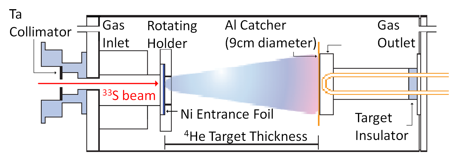
Figure 1: (color online) The gas cell used during activations. The insulator electrically isolated the gas cell from rest of beamline. A 9 cm diameter aluminum foil was used to catch the forward-recoiled ³⁶Cl atoms. The target holder could be isolated from the rest of the chamber and used as a Faraday cup during beam tuning with the target insulator. The target insulator was then removed during activations and the entire gas cell was used as a Faraday cup.

Before each sample activation, a beam current integration was performed with the target insulator installed and Ni entrance foil removed (see Fig. 1) and normalized to the current measured on a Faraday cup located $\sim$ 0.5 m upstream, to monitor any changes in source output. A second beam current integration was performed with target insulator removed and the Ni entrance foil in place and again normalized to the current measured on the upstream Faraday cup. The agreement between the two measurements was between $\sim$1-6% for all activation energies. This beam-tune dependent charge collection of the gas cell was included in the incident ³³S ion flux uncertainty. An additional 2% uncertainty was included in the number of incident ³³S ions from the lab Faraday cups and gas cell readouts.

The activation times, average electrical beam current on target, and integrated number of incident ³³S ions for each sample are summarized in Table 1. Sample S5 was previously activated and measured as a proof of principle sample Bowers et al. (2013). This sample’s activation procedure was identical to that of the samples discussed in this paper.

Table 1: Integrated beam current data for the ³⁶Cl activations.

Sample	t (hr)	I${}_{\text{avg}}$ (nA)	N33 ($10^{14}$)
S1	43.16	104.4	145(12)
S2	19.39	72.4	39.5(12)
S3	5.97	68.5	13.1(5)
S4	1.92	94.9	5.11(14)
S5	77.71	37.3	724(41)
S6	2.98	12.4	0.83(5)

To determine the energy range of the measured cross sections, the energy loss in the nickel entrance foil was experimentally determined, while the energy loss in the ⁴He target was calculated with the SRIM program Ziegler and Biersack (2011). To measure the energy loss in the nickel foil, the energy spectrum of the beam was measured with and without the nickel foil on a Si detector. The measurements were repeated for each activation energy.

The energy range for each activation was determined to be $E_{low}$ to $E_{high}$:

$$E_{high}=E_{foil}+\frac{FWHM}{2}$$ (1)

$$E_{low}=E_{gas}-\frac{FWHM}{2},$$ (2)

where $E_{foil}$ and $FWHM$ are the centroid and full width at half maximum, respectively, of the beam energy measured after the Ni entrance foil. $E_{gas}$ is the energy of the beam after the ⁴He gas target, evaluated by subtracting the energy loss in the gas calculated with SRIM from $E_{foil}$. The stopping power of the ⁴He gas was assumed to be constant through the gas cell because of the low pressure used and small beam currents on target ($<$ 100 nA, see Table 1). The cross sections are an average over the energy range $\Delta E=E_{high}-E_{low}$. There is a $\sim$20% ($\sim$0.2 MeV) uncertainty of the calculated stopping power of heavy ions in gases using SRIM. However, the SRIM uncertainty is an order of magnitude lower than the measured energy spread of the beam, which dominates the energy range. An example energy loss measurement is shown in Fig. 2, with the results summarized in Table 2.

Table 2: Results of the measured and calculated ³³S ions’ energy loss in the ⁴He gas cell. All energies are given in MeV.

Sample	E${}_{\text{i}}$	FWHM	E${}_{\text{foil}}$	E${}_{\text{gas}}$	E${}_{\text{high}}$	E${}_{\text{low}}$	$\Delta$E
S1	56	2.4	26.2	24.3	27.4	23.1	4.3
S2	63	2.6	33.3	31.5	34.6	30.2	4.4
S3	72	2.6	43.1	41.4	44.4	40.1	4.3
S4	81	2.6	52.9	51.3	54.2	50.0	4.2
S5	90	2.7	62.8	62.0	64.2	60.7	3.5
S6	104.5	2.8	78.4	77.0	79.8	75.6	4.2

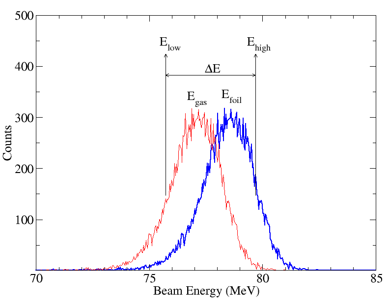
Figure 2: (color online) An example (sample S6) of the measured and calculated energy loss of ³³S ions in the gas cell. E${}_{\text{foil}}$ and E${}_{\text{gas}}$ are the centroids of the beam energy after the Ni entrance foil and ⁴He gas, respectively. The thick (blue) curve is the energy spectrum of the ³³S ions after passing through the nickel foil. E${}_{\text{high}}$ is the high energy end of the FWHM of the peak. The thin (red) curve is the bold curve shifted lower in energy by 1.44 MeV, the calculated energy loss in the ⁴He gas from SRIM, assuming constant stopping power over the energy spread. E${}_{\text{low}}$ is the low energy end of the FWHM of the shifted peak. The derived cross sections are thus averaged over the energy range $\Delta$E.

To ensure the ³⁶Cl atoms were collected in the catcher foil, a TRIM simulation was used to determine the dispersion of the beam through the gas cell. The simulation tracked $10^{4}$ ³³S ions passing through the Ni entrance foil, 10 Torr of ⁴He gas (5 Torr for sample S5), and embedded in the Al catcher foil. For all energies, greater than 99% of ions were collected within the Al catcher foil’s 9 cm diameter opening. An example of one of the simulations is shown in Fig. 3.

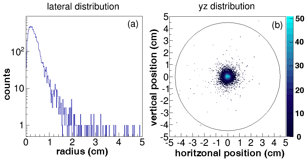
Figure 3: (color online) TRIM simulation of $10^{4}$ ³³S ions through the ⁴He-filled gas cell for sample S6. Figure (a) is a histogram of the lateral distribution of the implanted ions. The beam, before dispersion, is centered at a radius = 0. Figure (b) is a 2-D histogram of the particles implanted into the aluminum catcher foil. The circle is the 9 cm diameter opening of the Al catcher foil.

II.2 Chemical Processing

The Al catcher foils were chemically processed at Purdue University’s PRIME lab Vogt et al. (1994). In addition to the 5 activated samples, 2 identical, but non-irradiated foils were processed as blanks for the AMS measurement. The foils were cut into 8 pieces, put in separate containers, and mixed with stable chlorine carrier (1.101 mg/g chlorine concentration), where the precise Cl-carrier masses for each sample is given in Table 3. The addition of the Cl carrier fixes the ³⁶Cl/Cl ratio in each sample since both the ³⁶Cl and stable chlorine are recovered with the same efficiency. Twenty mL HNO₃ (trace metal grade, 70% concentration) were added to each sample to dissolve the foils. Since aluminum oxidizes in nitric acid, which inhibits its dissolution, 10 mL of HF (40% concentration) were added to prevent oxidation. Then, 45 mL of 18 M$\Omega$ DI H₂O were added to slow down the reaction. After one hour, an additional 20 mL of HNO₃ were added to the samples and left overnight to dissolve. Before decanting the solution in separate vials, 10 drops ($\sim$0.5 mL) of AgNO₃ were added to precipitate the Cl as AgCl and the aliquots were centrifuged. The excess solution was decanted, leaving behind the precipitated AgCl. The samples were finally baked for 2 days at 70^∘  C to remove any excess moisture. Since the AMS system at the University of Notre Dame can separate ³⁶Cl from its stable isobar, ³⁶S, there was no need to chemically reduce the sulfur in the samples (section II.3). Sample S5 was chemically processed in a similar protocol to that described above Bowers et al. (2013).

The number of chlorine carrier atoms added to each sample ($N_{\text{Cl}}$) was calculated by

$$N_{\text{Cl}}=\frac{m_{carrier}\times\left(1.101\text{ mg/g}\right)\times N_{A}}{M_{\text{Cl}}\times 1000\text{ mg/g}},$$ (3)

where $m_{carrier}$ (g) is the mass of the Cl carrier added to the sample, $N_{A}$ (=$6.02\times 10^{23}$ atoms/mol) is Avagadro’s number, and $M_{\text{Cl}}$ (=35.4527 g/mol) is the atomic weight of chlorine. The carrier mass was multiplied by 1.101 mg/g to arrive at the mass of chlorine added to each sample. The Cl carrier mass and number of atoms added to each sample are given in Table 3. The uncertainty in carrier mass, chlorine concentration, and chlorine recovery is estimated at 1%.

Table 3: The carrier mass and number of Cl atoms added to each sample.

Sample	m${}_{\text{carrier}}$ (g)	N${}_{\text{Cl}}$ ($10^{20}$)
S1	12.4643	2.33(2)
S2	12.4309	2.32(2)
S3	12.6888	2.37(2)
S4	12.6008	2.36(2)
S5	49.9923	9.35(9)
S6	12.7232	2.38(2)
Blank1	12.5357	2.34(2)
Blank2	10.2885	1.92(2)

II.3 AMS measurement

The ³⁶Cl/Cl ratio in the samples was measured with the AMS system at the University of Notre Dame Robertson et al. (2007, 2008). The system uses a converted Browne-Buechner spectrograph with a 1 m radius, single-dipole magnet. Ion position and energy loss are measured after the spectrograph with a parallel grid avalanche counter (PGAC) and ionization chamber (IC), respectively. The detector system is described in Robertson et al. (2008).

The difficulty in measuring ³⁶Cl arises from the need to separate it from its stable isobar, ³⁶S. To separate ³⁶Cl from ³⁶S, we used the Gas- Filled Magnet (GFM) approach Paul et al. (1989), since conventional electro-magnetic beamline elements are unable to separate the two isobars. In the GFM, the ³⁶Cl and ³⁶S ions separated into two different atomic number-dependent mean charge state groups and are bent in the GFM with different radii. The resulting peaks can then be distinguished in the position-sensitive PGAC. To achieve this separation the spectrograph was filled with 2.3 Torr of N₂ gas, which was isolated from the rest of the beamline with a 350 $\mu$g/cm² Mylar window. Count rates are kept low by physically blocking the ³⁶S beam from the detector with a movable shield. Figure 4 shows spectra of the standard, blank and an activated sample, where ³⁶Cl is separated from ³⁶S in both position and energy. A more detailed discussion of the detector settings can be found in Bowers et al. (2013).

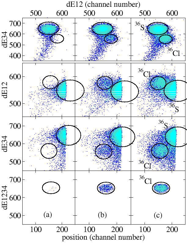
Figure 4: (color online) Identification spectra of ³⁶Cl . The left column (a) is a 15 minute measurement of Blank1. The middle column (b) is a 15 minute measurement of activated sample S6. The right column (c) is a 10 minute measurement of the standard (³⁶Cl/Cl = $4.16\times 10^{-11}$ ). The top row shows the separation of the ³⁶Cl and ³⁶S groups in energy loss in the first two anodes (dE12) in the ionization chamber (IC), plotted versus energy loss the last two anodes (dE34). The second and third rows plot the position of the groups versus dE12 and dE34, respectively. The sharp cutoff of the ³⁶S group is due to the beam shield, which blocked the majority of the ³⁶S beam from entering the detector. The bottom row shows spectra of position versus total energy loss(dE1234) in the IC. The spectra are gated on the ³⁶Cl groups in the top three rows’ spectra. The counts in the ³⁶Cl group from the blank sample come from the tail and spread of the much more intense ³⁶S beam.

The AMS measurement was performed with a Cl beam energy of 74.7 MeV and 8⁺ charge state. The blank samples were measured multiple times to determine the background level and detection limit. The samples were then measured in multiple and independent measurements in order of increasing predicted ³⁶Cl concentration to limit any potential source memory effects. The Blank1 sample was measured in between each measurement of activated samples. Blank2 verified the background levels determined with Blank1. The ³⁵Cl beam current was recorded on Farady cup 1 (FC1) (See Fig. 5), before and after each ³⁶Cl counting measurement, to normalize yields to source output. A summary of the blank measurements is shown in Fig. 6. Individual measurement times varied from 10 to 60 minutes, depending on ³⁶Cl concentration and source output.

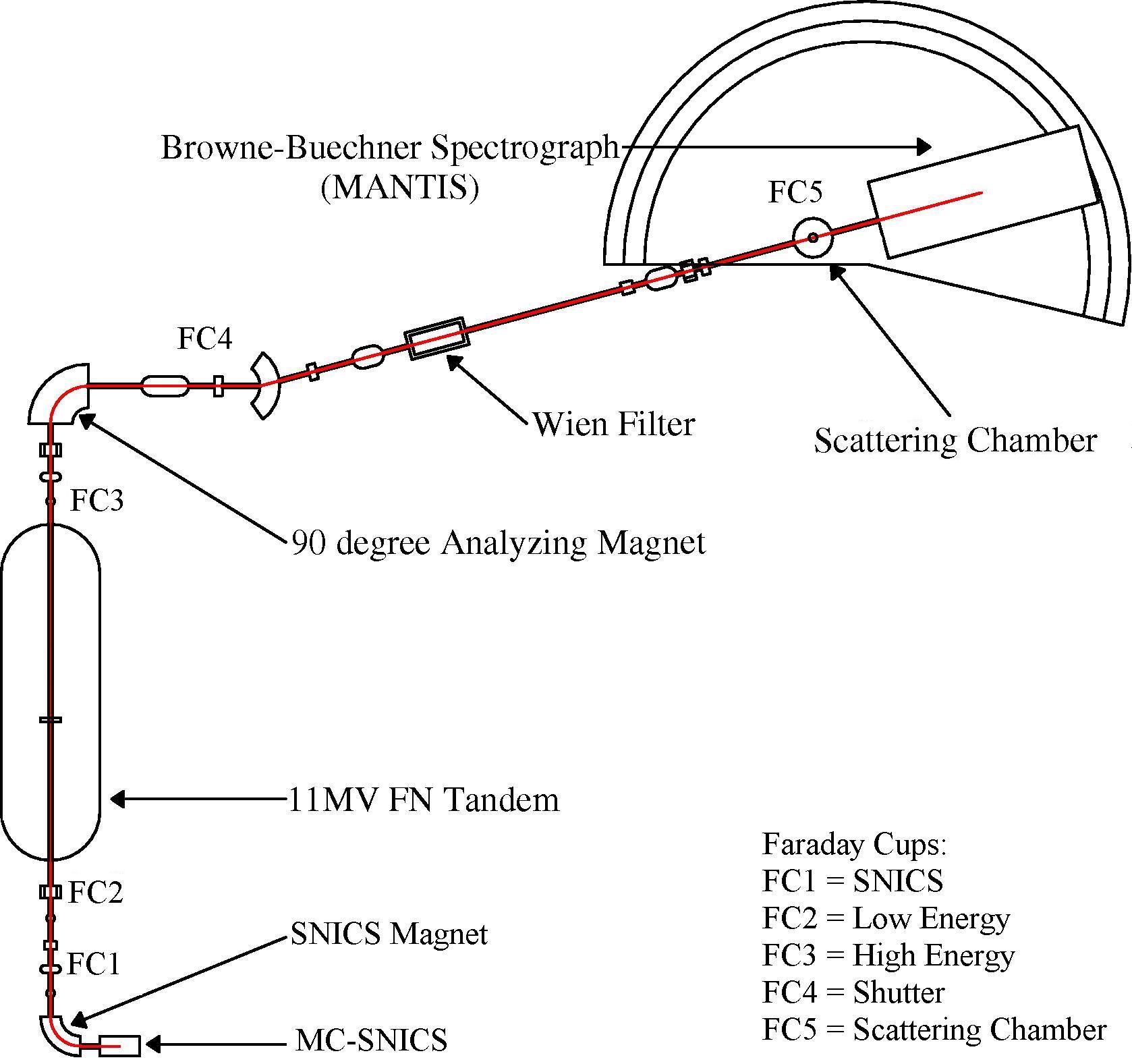
Figure 5: Diagram of the AMS beamline.

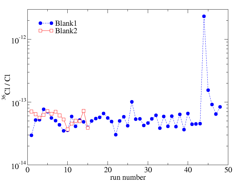
Figure 6: (color online) Background measurements performed with Blank1 (circles) and Blank2 (squares). Yields of ³⁶Cl for the activated samples were corrected for blank levels measured before each activated sample. Memory effects are seen in the spike at run 44, as it was the first blank measurement after the standard (³⁶Cl/Cl = $4.16\times 10^{-11}$ ) was measured. The ³⁶Cl count rate decreased back to normal background levels after $\sim$1 hr.

The transmission was measured with the ³⁵Cl beam currents on Faraday cups FC1 to FC5 (Fig. 5) between each sample measurement ($\epsilon_{35}$). This required reducing the beam output at the ion source ($<$ 1$\mu$A) before sending the beam through the accelerator. The transmission was also measured with ³⁶Cl in the detector with a standard, ³⁶Cl/Cl = $4.16\times 10^{-11}$ , and accounted for beamline and gating losses, and detector efficiency ($\epsilon_{36}$). The ³⁶Cl standard was obtained from Prime Lab and was originally prepared from an aliquot of a dilution series of NBS SRM 4422L Vogt et al. (1994). An uncertainty of 2% is assigned to the standard from uncertainty in the original reference material activity and subsequent AMS measurements of the standard Vogt et al. (1994). The ³⁶Cl/Cl ratio of the activated samples was normalized to the standard. For each sample, the transmission measured with the standard ($\epsilon_{36}$) was scaled to the transmissions measured with the ³⁵Cl beam between sample measurements ($\epsilon_{35}$) by

$$\epsilon_{36,sample}=\epsilon_{36,standard}\left(\frac{\epsilon_{35,sample}}{\epsilon_{35,standard}}\right).$$ (4)

The statistical variation in the standard measurements to obtain the transmission was 4%.

The ³⁶Cl/Cl measurements are summarized in Fig. 7 and Table 4. The ³⁶Cl/Cl values are the unweighted mean of the different measurements of each sample. The uncertainty is given as one standard deviation of the mean. The previously activated and measured sample, S5, was remeasured to obtain a more accurate result and used as a test for the reproducibility of the AMS measurement. The remeasured value of S5, ³⁶Cl/Cl = $(6.4\pm 0.3)\times 10^{-12}$, is in excellent agreement with the previously measured value of $(6.2\pm 1.1)\times 10^{-12}$ Bowers et al. (2013). Sample S1 showed no excess of ³⁶Cl above the blank level, so its result is quoted as an upper limit.

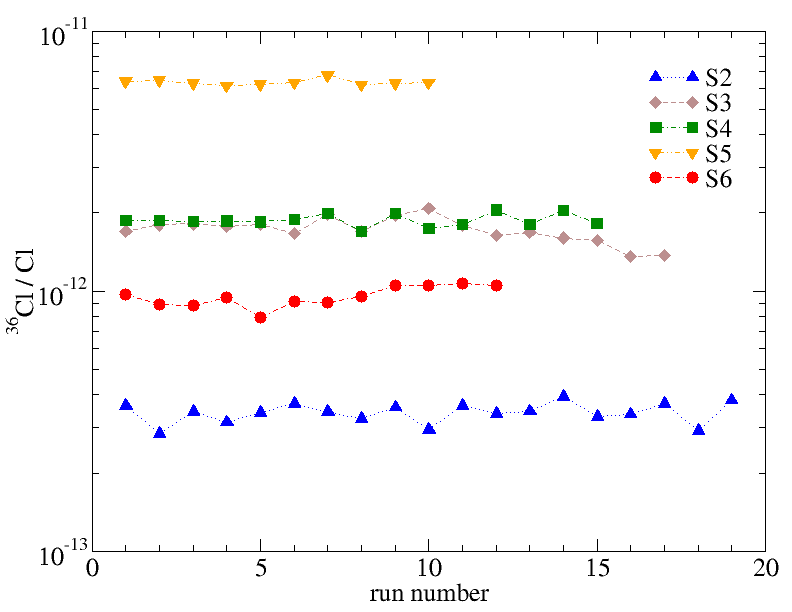
Figure 7: (color online) A summary of the activated sample measurements: S2 (upright triangles), S3 (diamonds), S4 (squares), S5 (upside down triangles), and S6 (circles). Sample S1 showed no excess ³⁶Cl above the blank level and is not shown.

Table 4: Results of the experimentally determined average cross sections.

Sample	E${}_{\text{low}}$ - E${}_{\text{high}}$	36Cl/Cl	N${}_{{}^{36}\text{Cl}}$	$\left<\sigma\right>$
	(MeV/A)		($10^{8}$)	(mb)
S1	0.70 - 0.83	$5\times 10^{-14}$	0.12	0.1
S2	0.92 - 1.05	$3.4(3)\times 10^{-13}$	0.79(8)	2.4(3)
S3	1.22 - 1.35	$1.7(2)\times 10^{-12}$	4.0(5)	37(5)
S4	1.51 - 1.64	$1.9(1)\times 10^{-12}$	4.5(3)	105(8)
S5	1.84 - 1.95	$6.4(3)\times 10^{-12}$	59.8(32)	199(16)
S6	2.29 - 2.42	$9.6(9)\times 10^{-13}$	2.3(2)	330(40)

III Results

The cross section was determined by

$$\left<\sigma\right>=\frac{N_{{}^{36}\text{Cl}}}{N_{33}\times N_{T}},$$ (5)

where $N_{33}$ is the total number of incoming ³³S ions during the activation (Table 1). The number of ³⁶Cl atoms in the sample ($N_{{}^{36}\text{Cl}}$) was found by multiplying N${}_{\text{Cl}}\times^{36}\text{Cl}/\text{Cl}$, determined from the chemical processing and AMS measurement, respectively. The area density of the ⁴He target atoms ($N_{T}$) is given by

$$N_{T}=\rho_{atm}\left(\frac{P}{P_{atm}}\right)\left(\frac{N_{A}}{M_{\text{He}}}\right)d,$$ (6)

where $N_{T}$ is given in units of target nuclei/cm², $\rho_{atm}$ (=0.1664 g/cm³) is the density of ⁴He at atmosphere, $P$ and $P_{atm}$ (Torr) are the pressure in the gas cell and atmospheric pressure, respectively. $M_{\text{He}}$ is the atomic weight of helium (=4.0026 g/mol) and $d$ (=24 cm) is the length of the gas cell from the Ni entrance foil to Al catcher foil. The experimentally determined cross sections are given in Table 4 along with their associated energy ranges (now expressed in MeV/A).

A summary of the uncertainties in the measurement is given in Table 5.

Table 5: Sources of uncertainty.

	Statistical	Systematical
Incident 33S ions (N33)		1-6% + 2%
Stable Cl carrier atoms (N${}_{\text{Cl}}$)		1%
4He target density		2.1%
AMS measurement
Standard	4%	2%
36Cl/Cl	3-11%	6%

IV Discussion

IV.1 Comparison with Theoretical Predictions

In order to evaluate the effect of the experimentally measured cross section on calculated ³⁶Cl production in the Early Solar System, the experimental cross sections were compared to theoretical predictions, including those used in two ESS irradiation models Goswami et al. (2001); Gounelle et al. (2006). In addition, the cross sections were also compared to the statistical model codes TALYS (using the default parameters, see below) Koning et al. (2008); Koning and Delaroche (2003) and NON-SMOKER Rauscher and Thielemann (2000, 2001), that calculate cross sections with the Hauser-Feshbach model. The comparison of the experimental data to the theoretical cross sections are shown in Fig. 8.

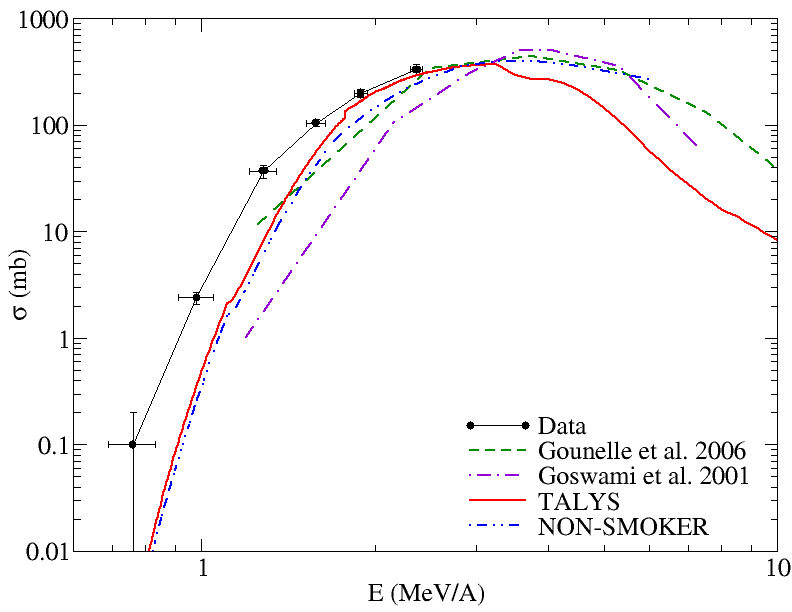
Figure 8: (color online) Comparison of the measured cross section and theoretical cross sections used in the ESS irradiation models from Gounelle et al. (2006) and Goswami et al. (2001), and calculated with NON-SMOKER Rauscher and Thielemann (2000, 2001) and TALYS Koning et al. (2008); Koning and Delaroche (2003).

Over the measured energy range all of the theoretical predictions are lower than the data. The measured cross section is over an order of magnitude higher than that used in Goswami et al. 2001 at low energy ($<$2 MeV/A). The discrepancy improves with increasing energy yet fails to be resolved. The Gounelle et al. 2006 cross sections were also under predicted. However, the deviation between experiment and theory is resolved with the highest energy data point (sample S6). This would mean that these irradiation models under-calculated the ³⁶Cl production via the ³³S($\alpha$,p) reaction. Section IV.2 discusses the potential effects of the experimental cross sections on ³⁶Cl production.

Though differences between the results of various codes and the data tends to diminish with increasing energy, TALYS and NON-SMOKER predictions give, in general, a better description of the experimental excitation curve than the cross sections used in the irradiation models. Below $\approx$ 2.3 MeV/A there is a good agreement between TALYS and NON-SMOKER calculations, with differences not exceeding a factor of 1.25. At higher energies, where no experimental data exists, TALYS cross section predictions drop off more rapidly than other model calculations due to the inclusion of additional reaction channels.

The NON-SMOKER calculations were obtained using level densities given by the constant temperature plus back-shifted Fermi gas (CT+BSFG) model Gilbert and Cameron (1965), where the back shift and level density parameters are from Rauscher et al. (1997). In terms of the optical model potential (OMP), the NON-SMOKER calculations have been performed using the semi-microscopic neutron and proton OMP from Jeukenne et al. (1977); Lejeune (1980) (JLM), with an $\alpha$-OMP given by McFadden and Satchler (1966) (MS). TALYS uses the CT+FG model as the default prescription for the level densities. To test the sensitivity of the TALYS results to the choice of level density model, identical calculations were performed using the CT+BSFG and BSFG models. Over the energy range covered by the experimental data, agreement between the two level density model calculations was found to be within 5%. Similarly, identical calculations were also performed using two different optical model potentials (OMP). By default TALYS uses a phenomenological OMP, based on smooth energy-dependent forms for the potential depths, where widths and diffusenesses are from global averages Koning and Delaroche (2003). Results given by this model were compared to those obtained using the JLM model. The JLM results were found to be enhanced by at most 20%. Cross section calculations were also performed using the MS $\alpha$-OMP. For energies below 1.6 MeV/A, the MS cross section predictions were reduced by approximately 20%. Above this incident energy, differences between the MS and default OMP calculations become negligible.

In summary, it was found that over the measured energy range TALYS systematically under-predicts the experimental data, a finding that is not sensitive to either the OMP, $\alpha$-OMP, or level density model choice.

IV.2 ³⁶Cl Production in the Early Solar System

While previous studies of ³⁶Cl in the early Solar System sought to reproduce the initial (³⁶Cl/³⁵Cl)₀ ratio inferred from meteorite measurements Goswami et al. (2001); Leya et al. (2003); Gounelle et al. (2006), here we examine the effects of using the measured ³³S($\alpha$,p) cross section compared to using the theoretically predicted values, as well as investigate how the astrophysical environment parameters affect which reactions are most important to ³⁶Cl production. The study was performed by adapting the irradiation model developed by Gounelle et al. 2001 Gounelle et al. (2001) and subsequently used by Gounelle et al. 2006 Gounelle et al. (2006). To ensure the calculations were consistent with the previous studies the same parameters were used (see case 2d from Gounelle et al. (2001)). This was the adopted case used by Gounelle et al. 2006 Gounelle et al. (2006).

When considering the possible radiation emitted from the protoSun, the particles’ energy spectrum and abundances must be established. The proton number flux was represented by a power-law distribution $\propto E^{-p}$, where $E$ is the proton energy in MeV/u and $p$ varies between 2.7 and 5. The ⁴He/¹H and ³He/¹H ratios scaled the proton number flux to give ⁴He and ³He fluxes. The Solar energetic particles (SEPs) originate from either impulsive (IMP) or gradual (GRD) events. Impulsive events are characterized by a sharper energy spectrum (larger $p$) and the presence of a ³He flux. Gradual events have a shallower energy spectrum (smaller $p$) and lack ³He. Three spectral parameter events (2 impulsive and 1 gradual) were taken from Gounelle et al. 2006 Gounelle et al. (2006) and one impulsive event from Leya et al. 2003 Leya et al. (2003). The four event settings used in this study are summarized in Table 6.

Table 6: Event parameters used in the irradiation calculations.

Event	p	4He/1H	3He/1H
IMP4	4	0.1	0.3
IMP5	5	0.1	0.3
IMPL	4	0.05	0.05
GRD	2.7	0.1	0

The reaction cross sections on S, Cl, and Ca targets were calculated with TALYS with the default parameters for the code and are shown in Fig. 9. The experimental data ($<$2.4 MeV/A) is combined with the TALYS calculations for the ³³S($\alpha$,p) reaction.

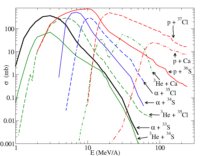
Figure 9: (color online) The TALYS calculated cross sections for the ³⁶Cl production reactions considered. The experimental data is included in the low energy sections of the ³³S($\alpha$,p)³⁶Cl reaction.

The calculations were performed with the TALYS cross sections and with the experimental data included with the TALYS predictions for all four events. The increase in production of ³⁶Cl from the ³³S($\alpha$,p) reaction along with the total increase in production, including all reaction channels, is shown in Fig. 10. The effects are most dramatic for the IMP5 event where the particle flux is highest where the cross section has been measured. However, the increase in total production is $<7\%$ for all events. Although the measured cross sections are larger than theoretically predicted by as much as a factor of 3 for some energies, the overall effect on ³⁶Cl production is minimal. As a check, the same calculations were performed with targets of a single chondritic elemental abundance. The results were consistent with the core-mantel composition since most of the particles are stopped in the mantle, where the volatile targets Cl and S are located. While the total effect of the measured cross sections on ³⁶Cl are small, the results do show that the effect can vary depending on the event parameters.

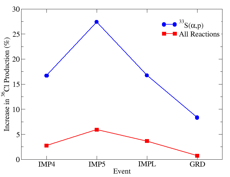
Figure 10: (color online) The increase in production of ³⁶Cl via the ³³S($\alpha$,p)³⁶Cl reaction as well as total production including all reactions using the experimental cross sections.

The effects of the various event parameters on the relative contributions of each individual reaction channel were tested, where the ³⁶Cl produced via one reaction is divided by the total ³⁶Cl produced for an event type. Fig. 11 shows the relative contributions of each reaction considered in the calculations. The most dominant channels for ³⁶Cl production are via the ³⁴S(³He,p), ³⁴S($\alpha$,pn), and ³³S($\alpha$,p) reactions. However the relative contributions of these reactions change substantially depending on the type of event considered. Reactions on ³⁴S targets contribute more to ³⁶Cl production than on ³³S targets due to its larger isotopic abundance (4.21% versus 0.75%). In the absence of ³He and a shallower energy spectrum in the GRD event case the Ca(p,x) reactions start to contribute a substantial fraction of the ³⁶Cl , which was not considered in Gounelle et al. (2006). In most cases, reactions on volatile targets like sulfur contribute the most to ³⁶Cl production in the early Solar System.

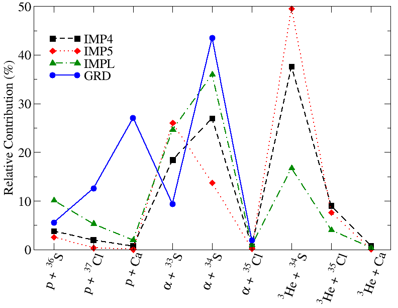
Figure 11: (color online) The relative contributions to the production of ³⁶Cl of individual reaction channels for a particular event.

V Conclusion

We have presented the first experimental results for the ³³S($\alpha$,p)³⁶Cl reaction. The cross section was measured at 6 energies between 0.70 - 2.42 MeV/A. The experimental results were shown to be lower than the theoretical predictions previously used in early Solar System irradiation models Goswami et al. (2001); Gounelle et al. (2006). The results were also compared to the TALYS and NON-SMOKER Hauser-Feshbach codes, where these calculations also under predict the experimental values. The OMP, $\alpha$-OMP, and LD model were varied using the TALYS code to try and resolve the discrepancy among the TALYS, NON-SMOKER, and the experimental data. However, it was found that the disagreements were not sensitive to those input models. Higher energy data would be useful to help resolve the discrepancies among the different theoretical models for this reaction.

The experimental cross sections increase the contribution from the ³³S($\alpha$,p) reaction to ³⁶Cl production but have a minimal effect on total ³⁶Cl production. While the importance of the ³³S($\alpha$,p) reaction was not as great as previously predicted, it was shown to be one of the dominant production reactions. The relative contributions of the important ³⁶Cl-production reactions vary appreciably depending on the astrophysical event parameters. The results show the importance of reactions on volatile targets like sulfur, especially the ³⁴S(³He,p), ³⁴S($\alpha$,pn), and ³³S($\alpha$,p) reactions. Currently the ³³S($\alpha$,p) reaction is the only reaction of these experimentally measured. The TALYS predictions for the ³⁴S(³He,p) and ³⁴S($\alpha$,pn) reactions differ substantially from the cross sections calculated in Gounelle et al. (2001). Experimental investigation of these reactions would be important as the effects of these discrepancies are not trivial on ³⁶Cl production. In a gradual event environment reactions on Ca contribute considerably to ³⁶Cl production. The Ca(p,x) reactions have been experimentally measured Schiekel et al. (1996); Sisterson et al. (1997); Imamura et al. (1997).