HerMES: dust attenuation and star formation activity in UV-selected samples from $z\sim 4$ to $z\sim 1.5^{\dagger}$

Abstract

We study the link between observed ultraviolet luminosity, stellar mass, and dust attenuation within rest-frame UV-selected samples at $z\sim 4,3$, and 1.5. We measure by stacking at 250, 350, and 500 $\mu$m in the Herschel/SPIRE images from the HerMES program the average infrared luminosity as a function of stellar mass and UV luminosity. We find that dust attenuation is mostly correlated with stellar mass. There is also a secondary dependence with UV luminosity: at a given UV luminosity, dust attenuation increases with stellar mass, while at a given stellar mass it decreases with UV luminosity. We provide new empirical recipes to correct for dust attenuation given the observed UV luminosity and the stellar mass. Our results also enable us to put new constraints on the average relation between star formation rate and stellar mass at $z\sim 4,3$, and 1.5. The star formation rate-stellar mass relations are well described by power laws ($\mathrm{SFR}\propto M_{*}^{0.7}$), with the amplitudes being similar at $z\sim 4$ and $z\sim 3$, and decreasing by a factor of 4 at $z\sim 1.5$ at a given stellar mass. We further investigate the evolution with redshift of the specific star formation rate. Our results are in the upper range of previous measurements, in particular at $z\sim 3$, and are consistent with a plateau at $3<z<4$. Current model predictions (either analytic, semi-analytic or hydrodynamic) are inconsistent with these values, as they yield lower predictions than the observations in the redshift range we explore. We use these results to discuss the star formation histories of galaxies in the framework of the Main Sequence of star-forming galaxies. Our results suggest that galaxies at high redshift ($2.5<z<4$) stay around 1 Gyr on the Main Sequence. With decreasing redshift, this time increases such that $z=1$ Main Sequence galaxies with $10^{8}<M_{*}/\textrm{M}_{\odot}<10^{10}$ stay on the Main Sequence until $z=0$.

1 Introduction

Star formation is one the most important processes in galaxies, yet our understanding of it is far from satisfactory. While it is commonly recognised that the evolution of the large-scale structure of the Universe is linked to that of dark matter, which is driven by gravitation, baryonic physics is much more challenging. Having a good understanding of star formation would be a great piece to put in the puzzle of galaxy formation and evolution. The first step is to be able to measure accurately the amount of star formation itself for a large number of galaxies. This means we need to be able to build statistical samples with observables that are linked to the recent star formation activity. One of the easiest way to perform this is to consider rest-frame ultraviolet (UV) selected samples, as the emission of galaxies in this range of the spectrum is dominated by young, short-lived, massive stars (Kennicutt, 1998). Thanks to the combination of various observatories, building UV-selected samples is now feasible over most of the evolution of the Universe, from $z\sim 10$ to $z=0$ (e.g. Bouwens et al., 2012; Ellis et al., 2013; Martin et al., 2005; Reddy et al., 2012b). There is however one drawback to this approach, which is that the attenuation by dust is particularly efficient in the UV (e.g. Calzetti, 1997). As the absorbed energy is re-emitted in the far-infrared (FIR) range of the spectrum, it is necessary to combine both of these tracers to get the complete energy budget of star formation. The current observational facilities however are such that it is much easier to build large samples from the restframe UV than from the restframe IR over a wide redshift range. It is then useful to look at the FIR properties of UV-selected galaxies as a function of redshift in order to understand the biases inherent to a UV selection, to characterise for instance the galaxy populations probed by IR and UV selections, determine the amount of total cosmic star formation rate probed by a rest-frame UV selection, or the link between the level of dust attenuation (as probed by the ratio of IR to UV luminosities, Gordon et al., 2000) and physical properties. This approach has been successful by combining UV selections and Spitzer data at $z\la 1$ to study the link between dust attenuation and UV luminosity or stellar mass (Buat et al., 2009; Martin et al., 2007; Xu et al., 2007), as well as correlation with galaxy colors (Arnouts et al., 2013). By measuring the ratio between the cosmic star formation rate density estimated from IR and UV selections, (Takeuchi, Buat, & Burgarella, 2005) showed that the fraction of the cosmic star formation rate probed by a UV selection, without correction for dust attenuation, decreases from 50 per cent to 16 per cent between $z=0$ and $z=1$ Takeuchi, Buat, & Burgarella (2005). At $z>1.5$, Spitzer data probe the mid-IR range of the spectrum, which can lead to an overestimation of the IR luminosity (e.g. Elbaz et al., 2010). At these redshifts, Herschel (Pilbratt et al., 2010) data become particularly valuable for such projects. Reddy et al. (2012a) extended this kind of study by stacking $z=2$ Lyman Break Galaxies (LBGs) in Herschel/PACS (Poglitsch et al., 2010) images to investigate their dust attenuation properties: they estimated that typical UV-selected galaxies at these epochs have infrared luminosities similar to Luminous Infrared Galaxies (LIRGs, $10^{11}<L_{\rm IR}/\textrm{L}_{\odot}<10^{12}$). Burgarella et al. (2013) combined the measurements at $0<z<4$ of the UV (Cucciati et al., 2012) and IR (Gruppioni et al., 2013) restframe luminosity functions to infer the redshift evolution of the total (UV+IR) cosmic star formation rate and dust attenuation. In a previous study based on a stacking analysis of UV-selected galaxies at $z\sim 1.5$ in Herschel/SPIRE (Griffin et al., 2010) images, we showed that using a UV-selection at $z\sim 1.5$ with a proper correction for dust attenuation enables us to recover most of the total cosmic star formation activity at that epoch (Heinis et al., 2013).

It is also necessary to investigate the link between dust attenuation and a number of galaxy properties, in order to be able to accurately correct for dust attenuation, by providing empirical relations for instance. One of the most commonly used empirical relation in this context is based on the correlation between the slope of the UV continuum and the dust attenuation (Meurer, Heckman, & Calzetti, 1999). Such correlation has been observed for star-forming galaxies from high to low redshifts (e.g. Buat et al., 2005; Burgarella, Buat, & Iglesias-Páramo, 2005; Heinis et al., 2013; Reddy et al., 2010; Seibert et al., 2005). However, the common assumption that the relation derived from local starbursts (Calzetti, 2001; Meurer, Heckman, & Calzetti, 1999) is universal is questionable (Heinis et al., 2013; Hao et al., 2011) as the extinction curve is dependent on the dust geometry (e.g. Calzetti, 2001) and dust properties (e.g. Inoue et al., 2006). Moreover, the UV slope of the continuum encodes partly the star formation history of the galaxies (Boquien et al., 2012; Kong et al., 2004; Panuzzo et al., 2007), and the observed relation between the UV slope and the dust attenuation is also selection-dependent (Buat et al., 2005; Seibert et al., 2005).

It is then useful to turn towards other observables, which might provide better ways to correct for dust attenuation in a statistical sense. Dust attenuation is for instance not really well correlated with observed UV luminosity (e.g. Buat et al., 2009; Heinis et al., 2013; Xu et al., 2007). On the other hand, the correlation with stellar mass is tighter (e.g. Buat et al., 2012; Finkelstein et al., 2012; Garn & Best, 2010; Pannella et al., 2009; Xu et al., 2007). This is somewhat expected as the dust production is linked to the star formation history, through heavy elements production, and stellar mass in this context can be seen as a crude summary of star formation history.

Investigating the link between dust attenuation and stellar mass is interesting by itself, but getting a direct estimate of the IR luminosity implies that we can also derive the star formation rate (SFR) accurately. This means that we are able for instance to characterise the relation between the SFR and the stellar mass. By considering galaxy samples based on star-formation activity, we are actually expecting to deal with objects belonging to the so-called ‘Main Sequence’ of galaxies. A number of studies pointed out that there is a tight relation between the SFR and the stellar mass of galaxies, from high to low redshift (Bouwens et al., 2012; Daddi et al., 2007; Elbaz et al., 2007; Noeske et al., 2007; Wuyts et al., 2011). Galaxies on this Main Sequence are more extended than starbursts (Elbaz et al., 2011; Farrah et al., 2008; Rujopakarn et al., 2013), the latter representing only a small contribution, in terms of number density, to the global population of star forming galaxies (Rodighiero et al., 2011). The relation between SFR and stellar mass also seems to be independent of the environment of the galaxies (Koyama et al., 2013). While there is debate on the slope and scatter of this relation, it is definitely observed at various redshifts, with its amplitude decreasing with cosmic time (Iglesias-Páramo et al., 2007; Martin et al., 2007; Noeske et al., 2007; Wuyts et al., 2011). The mere existence of this relation raises a number of issues for galaxy formation and evolution, as it implies that galaxies experience a rather smooth star formation history.

In this paper, we take advantage of the combination of the multiwavelength data available within the COSMOS field (Scoville et al., 2007), with the Herschel/SPIRE observations obtained in the framework of the Herschel Multi-Tiered Extragalactic Survey key program (HerMES, Oliver et al., 2012). We are assuming here that the rest-frame FIR emission we measure originates from the dust responsible for the UV/optical attenuation. Indeed, the wavelength range covered by SPIRE is dominated by the emission of dust heated by stars, the contribution from dust heated by Active Galactic Nuclei being significantly lower at these wavelengths (Hatziminaoglou et al., 2010). Moreover, our UV-selection biases against galaxies dominated by old stellar populations, hence the FIR emission we measure is mostly due to the dust heated by young stellar populations.

We focus on three UV-selected samples at $z\sim 4,3$, and 1.5 (see Ibar et al., 2013, for a similar study based on H$\alpha$-selected sample at $z=1.47$). We revisit the relations between dust attenuation and UV luminosity as well as stellar mass, over this wide redshift range, using homogeneous selections and stellar mass determination. Our aim is to disentangle the link between dust attenuation and these two physical quantities, by directly measuring their IR luminosities thanks to Herschel/SPIRE data. We also put new constraints on the SFR-stellar mass relations from $z\sim 4$ to $1.5$, and use our results to discuss the star formation histories of Main Sequence galaxies.

This paper is organised as follows: in Sect. 2 we present the UV-selected samples we build from the multiwavelength data available in the COSMOS field. As most of the galaxies of these samples are not detected individually with Herschel/SPIRE, we perform a stacking analysis, and describe the methods we use in Sect. 3. We present our results in Sect. 4: we detail the relations between dust attenuation and UV luminosity (Sect. 4.1.2) and between dust attenuation and stellar mass (Sect. 4.2). We present in Sect. 4.4 the SFR-stellar mass relations for UV-selected samples we obtain at $z\sim 1.5,3$ and 4. We also investigate the link between dust attenuation and UV luminosity and stellar mass jointly (Sect. 4.3). We discuss these results in Sect. 5 and present our conclusions in Sect. 6.

Throughout this paper, we make the following assumptions: we use a standard cosmoslogy with $\Omega_{\rm m}=0.3$, $\Omega_{\Lambda}=0.7$, and $H_{0}=70\,$km s^-1 Mpc^-1; we denote far-UV (FUV) and IR luminosities as $\nu L_{\nu}$; use AB magnitudes, and consider a Chabrier (2003) Initial Mass Function (IMF). When comparing to other studies, we consider that no conversion is needed for SFR and stellar mass estimates between Kroupa (2001) and Chabrier (2003) IMFs. When converting from Salpeter (1955) IMF to Chabrier (2003) IMF, we divide $M_{*,\rm Salpeter}$ by 1.74 (Ilbert et al., 2010), and SFR_Salpeter by 1.58 (Salim et al., 2007).

2 Data samples

Table 1: Description of UV-selected samples

	Sample
	$z\sim 1.5$	$z\sim 3$	$z\sim 4$
mag. limit	$u^{*}=26$	$r^{+}=26$	$i^{+}=26$
$z_{\rm phot\,range}$	$1.2-1.7$	$2.75-3.25$	$3.5-4$
$\langle z_{\rm phot}\rangle$	1.43	2.96	3.7
$\left\langle\sigma(z_{\rm phot})\right\rangle$	0.04	0.1	0.17
$N_{\rm gal}$	42,184	23,774	7,713
$\lambda_{\rm rest\,eff}$[Å]	1609	1574	1623
$\log(L_{\rm FUV}(\langle z_{\rm phot}\rangle,\rm{mag.limit})[L_{\sun}])$	9.6	10.1	10.3
$\left\langle\sigma\left(\log(M_{*}[\textrm{M}_{\odot}])\right)\right\rangle$	0.15	0.27	0.30
$\log(M_{*}[\textrm{M}_{\odot}])$ reliability limit	9.5	10.3	10.6

2.1 Photometric redshifts and stellar masses

We base this study on the photometric redshift catalogue built from the COSMOS data by Ilbert et al. (2009, version 2.0). This catalogue is based on an $i$- band detection, down to 0.6$\,\sigma$ above the background (Capak et al., 2007). These estimates benefit from new near-infrared imaging in the $Y$, $J$, $H$, and $K_{s}$ bands obtained with the VISTA telescope as part of the UltraVISTA project (McCracken et al., 2012). In the redshift range $1.5<z<3.5$, the precision on the photometric redshifts (defined as the scatter of the difference with spectroscopic redshifts, in 1+$z$) is around 3 per cent. This value is given by Ilbert et al. (2013) for objects with $K_{s}<24$, and has been obtained by comparing to zCOSMOS faint sample ($I_{med}=23.6$) and faint DEIMOS spectroscopic redshifts ($I_{mean}=23.5$). At $z\sim 4$, the spectroscopic redshifts available ($I_{med}=24.4$) yield a precision of 4 per cents, and suggest that the contamination from low redshift galaxies is negligible. On the other hand, this spectroscopic sample at $z\sim 4$ is not likely to be representative of our sample at the same redshifts (see Table 1). The actual photometric redshift error for our samples might be larger than this, as we are dealing with fainter objects. We also quote in Table 1 as an alternative the mean photometric redshift error, in (1+z), estimated from the PDF of the photometric redshifts derived by Ilbert et al. (2009). Ilbert et al. (2010) showed that the error measured from the PDF is a robust estimate of the accuracy as measured with respect to spectroscopic objects. At $z\sim 3$, the mean error from the PDF is 0.1, and 0.17 at $z\sim 4$.

We also consider in this paper the stellar masses estimates of Ilbert et al. (2009, version 2.0). Briefly, the stellar masses are derived from SED fitting to the available photometry, assuming Bruzual & Charlot (2003) single stellar population templates, an exponentially declining star formation history, and the Chabrier (2003) IMF. Ilbert et al. (2013) showed that the assumption of an exponentially declining star formation history does not have a strong impact on the stellar masses estimates.

2.2 UV-selected samples

We consider three UV-selected samples at $z\sim 1.5$, $z\sim 3$, and $z\sim 4$. The sample at $z\sim 1.5$ has already been presented in Heinis et al. (2013). We detail here how we build the samples at $z\sim 3$, and $z\sim 4$. We use optical imaging of the COSMOS field from Capak et al. (2007) in $r^{+}$ and $i^{+}$, both from Subaru. We cross-match single band catalogues built from these images with the photometric redshift catalogue of Ilbert et al. (2009, version 2.0). Ninety-nine per cent of the objects with $u^{*}<26$ have a counterpart in the catalogue of Ilbert et al. (2009, version 2.0), while 92 per cent of objects with $r^{+}<26$ have a counterpart. In the $i^{+}$-band, we use directly the catalog of Ilbert et al. (2009, version 2.0), as it is based on an $i^{+}$-band detection.

We then build UV-selected samples, at $z\sim 3$ and $z\sim 4$. We detail in Table 1 the main characteristics of the three samples we consider here. All these samples probe the FUV rest-frame range of the spectrum, with rest-frame effective wavelengths within the range $1570-1620$ Å at the mean redshifts of the samples (see Table 1).

We will perform stacking at 250, 350 and 500 $\mu$m as a function of FUV luminosity, $L_{\rm FUV}$, and stellar mass $M_{*}$. We derive $L_{\rm FUV}$ from the observed magnitude as follows:

$$L_{\nu}=\frac{4\pi D_{L}^{2}(z)10^{-0.4(48.6+m)}}{1+z}$$ (1)

where $D_{L}(z)$ is the luminosity distance at $z$, and $m$ is the observed magnitude: we use $u^{*}$ at $z\sim 1.5$, $r^{+}$ at $z\sim 3$, and $i^{+}$ at $z\sim 4$. We then compute the UV luminosity at 1530 Å.

We estimate a reliability limit in stellar mass for each sample the following way. We compute, as a function of $M_{*}$, the fraction of objects with 3.6 $\mu$m flux measurements fainter than the 80 per cent completeness limit (2.5 $\mu$Jy, Ilbert et al., 2010). We choose the reliability limit as the minimum $M_{*}$ value where this fraction is lower than 0.3. In other words, above this value of $M_{*}$, the fraction of objects that have a flux at 3.6 $\mu$m larger than the 80% completeness limit is $\geq 0.7$. Note that we do not impose a cut on 3.6 $\mu$m fluxes. The stellar mass is also estimated for objects with 3.6 $\mu$m flux fainter than 2.5 $\mu$Jy, however this estimate is less robust than for brighter objects. We quote the reliability limits for each sample in Table 1.

3 Stacking measurements

We base our study on the Herschel/SPIRE imaging of the COSMOS field obtained within the framework of the HerMES key program(Oliver et al., 2012). Most of the objects from our UV-selected samples are not detected individually in these images, so we rely on a stacking analysis. We use the same methods as those presented in Heinis et al. (2013) to measure flux densities using stacking. We recall here only the main characteristics of the methods. We perform stacking using the IAS library (Bavouzet, 2008; Béthermin et al., 2010). We use mean stacking, without cleaning images from detected sources. We showed in Heinis et al. (2013) that using our method or median stacking with cleaning images from detected sources, yields similar results. We correct the stacking measurements for stacking bias, using extensive simulations of the detection process of the sources. We perform these simulations by injecting resolved artificial sources in the original images, and keeping track of the recovered sources. We then use the stacking of these artificial sources to correct the actual measurements. We also correct for the clustering of the input catalogue by taking into account the angular correlation function of the input sample.

We derive errors on the stacking flux densities by bootstrap resampling. We use hereafter the ratio of the stacking flux density over its error as a measurement of signal-to-noise ratio. For each stacking measurement, we obtain a flux density at 250, 350 and 500 $\mu$m. We derive an infrared luminosity $L_{\rm IR}$ by adjusting these fluxes to the Dale & Helou (2002) templates, using the SED-fitting code CIGALE (Noll et al., 2009). The Dale & Helou (2002) templates have been shown to be a reasonable approximation of the SEDs of Herschel sources (Elbaz et al., 2010, 2011). We consider $L_{\rm IR}$ as the integration of the SED over the range $8<\lambda<1000\,\mu$m. CIGALE estimates the probability distribution function of $L_{\rm IR}$. We consider the mean of this distribution as our $L_{\rm IR}$ value, and the standard deviation as the error on $L_{\rm IR}$. We use as redshift the mean redshift of the galaxies in the bin.

Hereafter, we perform stacking as a function of $L_{\rm FUV}$ and $M_{*}$ separately in Sect. 4.1.1, 4.1.2, 4.2, and 4.4, and we also perform stacking as a function of both $L_{\rm FUV}$ and $M_{*}$ in Sect. 4.3. We characterise each bin by the mean value of $L_{\rm FUV}$ and/or $M_{*}$. We derive the errors on the mean $L_{\rm FUV}$ using mock catalogues. These mock catalogues are only used to estimate errors on mean $L_{\rm FUV}$ and $M_{*}$. We build 100 mock catalogues, with new redshifts for each object, drawn within the probability distribution functions derived by Ilbert et al. (2010). We can then assign new $L_{\rm FUV}$ using eq. 1. For a given stacking measurement including a given set of objects, we compute the mean of $L_{\rm FUV}$ for each mock catalogue. The error on the mean $L_{\rm FUV}$ is then the standard deviation of the means obtained from all mock catalogues. We derive errors on the mean $M_{*}$ in a similar way, using the stellar mass probability distribution functions derived by Ilbert et al. (2010).

4 Results

We first show results of the stacking as a function of $L_{\rm FUV}$; we look at the relation between the average $L_{\rm IR}$ and $L_{\rm FUV}$ (Sect. 4.1.1) and then at the relation between the dust attenuation, probed by the IR to UV luminosity ratio, and $L_{\rm FUV}$ (Sect. 4.1.2).

We further turn to results we obtain by stacking as a function of stellar mass, looking at the relation between dust attenuation and stellar mass (Sect. 4.2). We also investigate the joint dependence between $L_{\rm FUV}$, $M_{*}$, and dust attenuation (Sect. 4.3).

As we obtain estimates of $L_{\mathrm{IR}}$, we derive a total star formation rate by combining with the observed UV luminosity, and look at the relation between star formation rate and stellar mass in our samples (Sect. 4.4).

4.1 Stacking as a function of $L_{\rm FUV}$ 

4.1.1 $L_{\rm IR}$ -$L_{\rm FUV}$ relation from $z\sim 4$ to $z\sim 1.5$

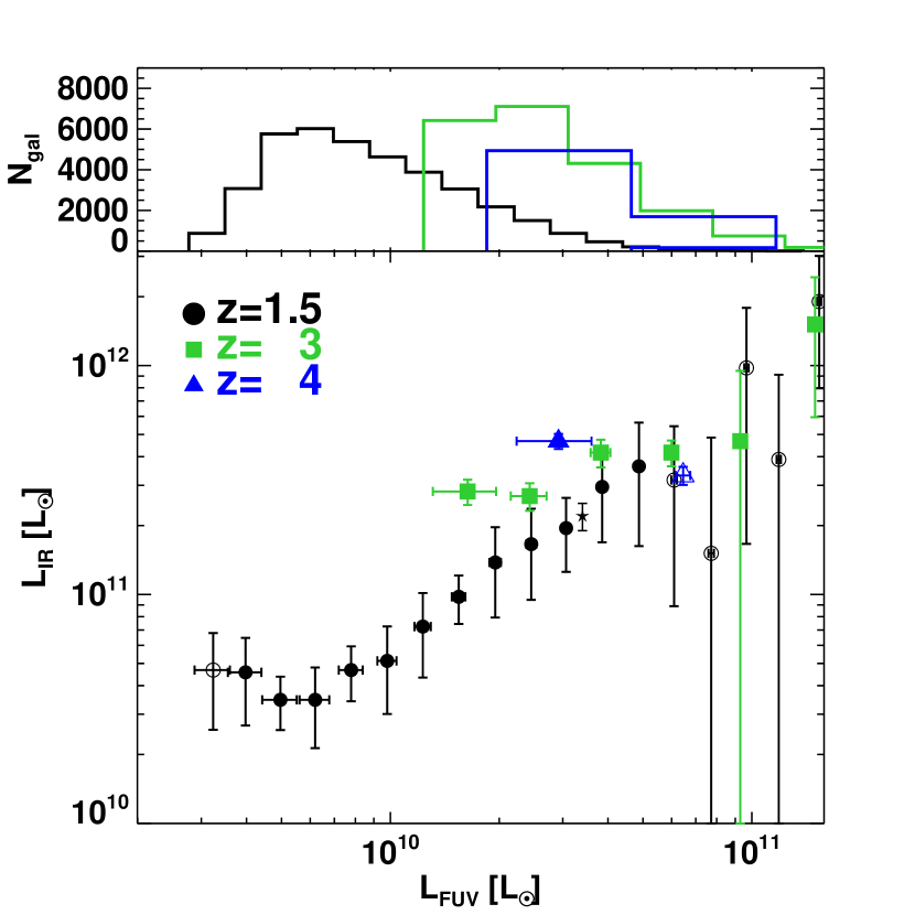
Figure 1: Top: histogram of the number of galaxies included in the stacking measurements at $z\sim 1.5$ (black), $z\sim 3$ (green), and $z\sim 4$ (blue). Bottom: $L_{\rm IR}$ versus $L_{\rm FUV}$, at $z\sim 1.5$ (from Heinis et al., 2013, black circles), $z\sim 3$ (green squares), and $z\sim 4$ (blue triangles). Filled symbols represent stacking measurements with $S/N>3$ in the three SPIRE bands, and open symbols measurements which do not meet this criterion. The star symbol show the result of stacking measurements by Reddy et al. (2012a) on a sample of Lyman Break Galaxies at $z=2$.

In Fig. 1, we show the $L_{\rm IR}$ measured by stacking as a function of $L_{\rm FUV}$ at $z\sim 1.5,3,$ and 4. At $z\sim 1.5$, for galaxies with $3\times 10^{9}<L_{\rm FUV}/\textrm{L}_{\odot}<8\times 10^{9}$, $L_{\rm IR}$ is roughly constant at $L_{\rm IR}\sim 4\times 10^{10}\textrm{L}_{\odot}$. For $L_{\rm FUV}$ brighter than $8\times 10^{9}\,\textrm{L}_{\odot}$, $L_{\rm IR}$ is increasing with $L_{\rm FUV}$, with a power law slope of $1.1\pm 0.2$. This shows that in this range of UV luminosities at $z\sim 1.5$, $L_{\rm IR}$ and $L_{\rm FUV}$ are well correlated.

At $z\sim 3$ and $z\sim 4$, the situation is quite different. At these redshifts, we explore a smaller dynamic range of UV luminosities, $10^{10}<L_{\rm FUV}/\textrm{L}_{\odot}<10^{11}$. At these epochs, we do not measure any statistically significant trend of $L_{\rm IR}$ with $L_{\rm FUV}$ in UV-selected samples. We find that $L_{\rm IR}$ is roughly constant at $L_{\rm IR}\sim 4\times 10^{11}\textrm{L}_{\odot}$.

4.1.2 Dust attenuation as a function of $L_{\rm FUV}$ from $z\sim 4$ to $z\sim 1.5$

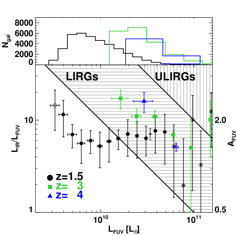
Figure 2: Top: histogram of the number of galaxies included in the stacking measurements at $z\sim 1.5$ (black), $z\sim 3$ (green), and $z\sim 4$ (blue). Bottom: IR to UV luminosity ratio versus $L_{\rm FUV}$, at $z\sim 1.5$ (from Heinis et al., 2013, black circles), $z\sim 3$ (green squares), and $z\sim 4$ (blue triangles). Filled symbols represent stacking measurements with $S/N>3$ in the three SPIRE bands, and open symbols measurements which do not meet this criterion. The right axis shows the equivalent attenuation in the FUV band, in magnitudes, using eq. 2. The horizontally hatched area represents the region where LIRGs are, and the vertically hatched area represents the same for ULIRGs. The star symbol show the stacking results of Reddy et al. (2012a) on a sample of Lyman Break Galaxies at $z=2$.

In Fig. 2, we show the relations between the $L_{\rm IR}/L_{\rm FUV}$ ratio, a proxy for dust attenuation, and $L_{\rm FUV}$ at $z\sim 3$ and $z\sim 4$. We also show for comparison the results we obtained at $z\sim 1.5$ (Heinis et al., 2013).

We indicate the equivalent dust attenuation in the FUV, $A_{\rm FUV}$, derived from the $L_{\rm IR}$ to $L_{\rm FUV}$ ratio using (Buat et al., 2005):

$$A_{\rm FUV} = -0.0333\rm{IRX}^{3}+0.3522\rm{IRX}^{2}+1.1960\rm{IRX}$$ (2)

$$+ 0.4967$$

$$\rm{IRX} = \log\left(\frac{L_{\rm IR}}{L_{\rm FUV}}\right).$$

In the ranges of UV luminosity we probe, the relations between dust attenuation and $L_{\rm FUV}$ change from $z\sim 4$ to $z\sim 1.5$. At $z\sim 1.5$, the dust attenuation is mostly independent of $L_{\rm FUV}$. At $z\sim 3$ and $z\sim 4$, we observe that the dust attenuation on average decreases with $L_{\rm FUV}$. This decrease is linked to the fact that $L_{\rm FUV}$ is not well correlated with $L_{\rm IR}$, as suggested by Fig. 1.

Our results also show that at given $L_{\rm FUV}$, dust attenuation is larger at $z\sim 3,4$ than at $z\sim 1.5$ for galaxies with $L_{\rm FUV}<4\times 10^{10}L_{\odot}$. We show later that this effect is actually linked to the stellar mass of the galaxies (see Sect. 4.3).

4.2 Dust attenuation as a function of stellar mass

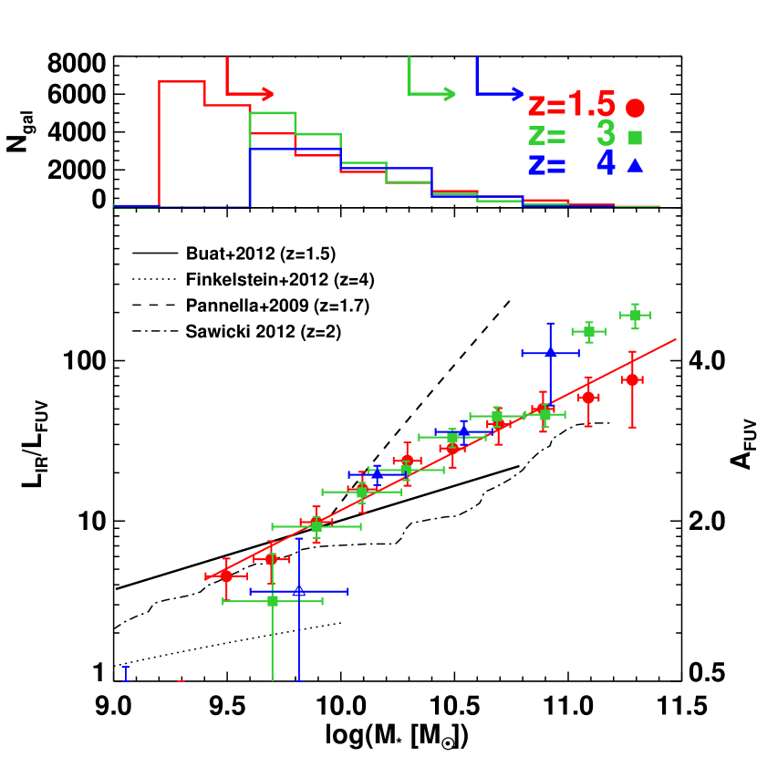
Figure 3: Top: histogram of the number of galaxies included in the stacking measurements at $z\sim 1.5$ (red), $z\sim 3$ (green), and $z\sim 4$ (blue). The arrows show the mass reliability limits for each sample. Bottom: IR to UV luminosity ratio versus stellar mass, at $z\sim 1.5$ (red circles), $z\sim 3$ (green squares), and $z\sim 4$ (blue triangles). The right axis shows the equivalent attenuation in the FUV band, in magnitudes, using eq. 2. The solid red line shows our fit to the $z\sim 1.5$ measurements. The various black lines show previous measurements at various redshifts from Buat et al. (2012, $z=1.5$), Finkelstein et al. (2012, $z=4$) (whose results agree really well with Bouwens et al. (2012, $z=4$), that we do not show here), Pannella et al. (2009, $z=2$), and Sawicki (2012, $z=2$).

We investigate here the relation between dust attenuation and stellar mass. We show in Fig. 3 our measurements of the ratio of IR to UV luminosity as a function of stellar mass, at $z\sim 4$, $z\sim 3$, and $z\sim 1.5$.

The link between dust attenuation and stellar mass is strikingly different from the link between dust attenuation and UV luminosity. At all the redshifts we consider here, there is a clear correlation, on average, between dust attenuation and stellar mass. The results in Fig. 3 show that the $L_{IR}/L_{FUV}$ ratio is much better correlated with stellar mass than with UV luminosity. Within the same samples, the $L_{IR}/L_{FUV}$ ratio varies by a factor of two at most as a function of $L_{\rm FUV}$, while it varies by one order of magnitude as a function of $M_{*}$. Our results also suggest that there is no significant evolution with redshift of the dust attenuation at a given stellar mass, between $z\sim 4$ and $z\sim 1.5$. There is a possible trend at the high mass range ($M_{*}>10^{11}\textrm{M}_{\odot}$) that dust attenuation decreases between $z\sim 3$ and $z\sim 1.5$. The statistics is however low for these mass bins, and the fraction of UV-selected objects directly detected at SPIRE wavelengths is the highest.

Assuming that the relation between the $L_{\rm IR}$ to $L_{\rm FUV}$ ratio and $M_{*}$ can be parameterised as:

$$\textrm{IRX}=\alpha\log\left(\frac{M_{*}}{10^{10.35}}\right)+\textrm{IRX}_{0}$$ (3)

we obtain as best fits parameters at $z\sim 1.5$ $\alpha=0.72\pm 0.08$ and $\textrm{IRX}_{0}=1.32\pm 0.04$. This relation is valid at $z\sim 1.5,3,$ and 4 for $10^{10}<M_{*}/\textrm{M}_{\odot}<10^{11}$.

We compare our results with previous estimates of the relation between dust attenuation and stellar mass for UV-selected samples. At $z\sim 1.5$, our results are in reasonable agreement with those from Buat et al. (2012), derived from SED fitting, based on UV-selected objects with spectroscopic redshifts and photometry from the restframe UV to the restframe FIR. Our results are also in good agreement with those from Whitaker et al. (2012) at $1.<z<1.5$, who studied a mass-selected sample of star-forming galaxies. Our findings are also consistent with those from Wuyts et al. (2011), who observed that the ratio of SFRs derived from the IR and the UV increases with total SFR ($=$SFR${}_{\mathrm{IR}}+$SFR _UV) and $M_{*}$. While we observe a higher amplitude at a given mass, our measurements show a slope of the IRX$-M_{*}$ relation similar to the one derived by Sawicki (2012), whose results are derived from SED fitting applied to a sample of BX galaxies at $z\sim 2.3$, using photometric redshifts, and UV/optical restframe data. We also compare our results at $z\sim 4$ with the measurements of Finkelstein et al. (2012), who studied the link between the slope of the UV continuum, $\beta$, and the stellar mass. We converted their measurements of $\beta$ to $A_{\rm FUV}$ assuming the Meurer, Heckman, & Calzetti (1999) relation, which has been claimed to be valid at $z=4$ (Lee et al., 2012). The measurements of Finkelstein et al. (2012) probe a lower mass range than ours, making a direct comparison difficult. Our measurement in the lowest mass bin we probe at $z\sim 4$ is in formal agreement with theirs, however it has a low signal to noise ratio, and may suffer from significant incompleteness in mass as well. Nevertheless, the extrapolation of the relation observed by Finkelstein et al. (2012) at higher masses does not match our measurements. We also compare our results with the relation derived by Pannella et al. (2009) at $z=2$, from radio stacking of a sample of BzK-selected galaxies. This relation would significantly overpredict the dust attenuation for a UV-selected sample when compared to our results. These different relations between dust attenuation and stellar mass for UV and BzK-selected samples coud be due to the fact that the BzK selection is less sensitive to dust attenuation, and probes galaxies that are dusty enough to be missed by UV selections (e.g. Riguccini et al., 2011). We note the more recent results from Pannella, Elbaz, & Daddi (2013) are in better agreement with our measurements.

4.3 Dust attenuation as a function of stellar mass and UV luminosity

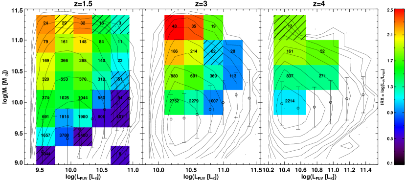
Figure 4: Dust attenuation as a function of stellar mass and UV luminosity at $z\sim 1.5$ (left), $z\sim 3$ (middle) and $z\sim 4$ (right). The color codes $\textrm{IRX}=\log(L_{\rm IR}/L_{\rm UV})$ in each cell where the stacking measurement is meaningful. Filled cells indicate stacking measurements with $S/N>3$ in the 3 SPIRE bands, while black hatched cells show measurements with at most two SPIRE bands with $S/N>3$. The number of galaxies contributing to the stacking is indicated in each cell. The contours show the distribution of galaxies in the $(L_{\rm FUV},M_{*})$ plane. The empty circles show the mean stellar mass for a given UV luminosity bin, with the dispersion as error bar.

The results presented in Sects. 4.1.2 and 4.2 show that dust attenuation is on average well correlated with stellar mass, and that this correlation is tighter than the correlation between dust attenuation and $L_{\rm FUV}$. However, dust attenuation is not completely independent of $L_{\rm FUV}$ : while at $z\sim 1.5$, dust attenuation is mostly constant for $5\times 10^{9}<L_{\rm FUV}/\textrm{L}_{\odot}<5\times 10^{10}$ it increases for fainter UV luminosities. On top of this, dust attenuation is higher at $z\sim 3$ than at $z\sim 1.5$ at the same $L_{\rm FUV}$, but is found to be decreasing with $L_{\rm FUV}$. It seems then that dust attenuation depends both on $L_{\rm FUV}$ and $M_{*}$, and that we need to investigate what is the link between dust attenuation and these two quantities.

We performed stacking as a function of $L_{\rm FUV}$ and $M_{*}$ at $z\sim 1.5,3,$ and 4, using binnings of $\left(\Delta\log(L_{\rm FUV}/\textrm{L}_{\odot}),\Delta\log(M_{*}/\textrm{M}_{\odot})\right)=(0.3,0.3),(0.3,0.4)$, and $(0.4,0.4)$ respectively. We show in Fig. 4 the result of the stacking as a function of UV luminosity and stellar mass. Note that filled cells indicate bins where the stacking measurements have $S/N>3$ in all SPIRE bands, hatched cells bins where there is at most two SPIRE band with $S/N>3$, and other cells are kept empty. These empty cells indicate that there is no robust stacking detection in these bins.

The measurements in Fig. 4 clearly show that dust attenuation depends both on $L_{\rm FUV}$ and $M_{*}$. Dust attenuation increases with $M_{*}$ at a given $L_{\rm FUV}$, while it decreases with $L_{\rm FUV}$ at a given $M_{*}$. We already observed an increase of the dust attenuation for faint UV galaxies (Heinis et al., 2013) at $z\sim 1.5$ (also observed previously by Buat et al., 2009, 2012; Burgarella et al., 2006). Indeed, galaxies with large stellar masses and strong dust attenuation exhibit faint UV luminosities, which is true for all redshifts we study here. The results in Fig. 4 also show that the range of dust attenuation values over the stellar mass range decreases with $L_{\rm FUV}$, as suggested in a previous study (Heinis et al., 2013). We also represent in Fig. 4 the location of the mean stellar mass for each UV luminosity bin. The results at $z\sim 1.5$ in particular show that lines of constant dust attenuation follow lines roughly parallel to this relation. This explains the global lack of dependence of dust attenuation with $L_{\rm FUV}$at $z\sim 1.5$ (Heinis et al., 2013). At $z\sim 3$ and $z\sim 4$, there is only a weak correlation between $M_{*}$ and $L_{\rm FUV}$. This implies that bins in $L_{\rm FUV}$ are mostly dominated by low mass galaxies in these samples. As shown in Fig. 4, the dust attenuation at a given mass decreases with $L_{\rm FUV}$, which is exactly what we observe when stacking as a function of $L_{\rm FUV}$ only.

The relation between dust attenuation and $(L_{\rm FUV},M_{*})$ also depends on redshift. Indeed, at a given mass and $L_{\rm FUV}$, the attenuation is higher at $z\sim 3$ than at $z\sim 1.5$. For instance, galaxies with $10^{10}\la L_{\rm FUV}/L_{\odot}\la 10^{10.35}$ have a dust attenuation roughly 0.2 dex larger at a given mass at $z\sim 3$ with respect to galaxies at $z\sim 1.5$. This, combined with slightly different $L_{\rm FUV}$ -$M_{*}$ relations explains why the dust attenuation for this range of UV luminosities is larger at $z\sim 3$ compared to $z\sim 1.5$ (see Fig. 2).

We can use the results presented above in order to provide empirical recipes to estimate dust attenuation as a function of $M_{*}$ and $L_{\rm FUV}$. We detail those in Appendix A.

4.4 Star formation rate-stellar mass relations from $z\sim 4$ to $z\sim 1.5$

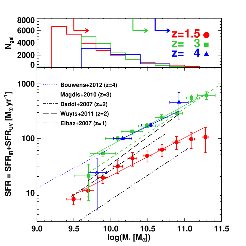
Figure 5: Top: histogram of the number of galaxies included in the stacking measurements at $z\sim 1.5$ (red), $z\sim 3$ (green), and $z\sim 4$ (blue). The arrows show the mass reliability limits for each sample. Bottom: star formation rate (sum of IR and FUV contributions) versus stellar mass, at $z\sim 1.5$ (red circles), $z\sim 3$ (green squares), and $z\sim 4$ (blue triangles). The various lines show previous measurements at various redshifts from Bouwens et al. (2012, $z=4$), Daddi et al. (2007, $z=2$), Elbaz et al. (2007, $z=1$), Magdis et al. (2010, $z=2$), and Wuyts et al. (2011, $z=2$).

Table 2: Fits to average star formation rate - stellar mass relations

	Sample
	$z\sim 1.5$	$z\sim 3$	$z\sim 4$
$\log(\textrm{SFR}_{0}\,[\textrm{M}_{\odot}\mathrm{yr}^{-1}])$	$-5.7\pm 0.7$	$-5.4\pm 0.4$	$-4.7\pm 1.0$
$\alpha$	$0.70\pm 0.07$	$0.73\pm 0.04$	$0.66\pm 0.10$

The fits are performed assuming that $\textrm{SFR}=\textrm{SFR}_{0}M_{*}^{\alpha}$.

The measurements presented above yield average estimates of $L_{\rm IR}$ as a function of stellar mass at $z\sim 1.5,3,$ and 4. We can combine these measurements with those of the observed, uncorrected UV luminosities to obtain a total star formation rate as:

$$\rm{SFR}=SFR_{\rm IR}+SFR_{\rm UV}$$ (4)

with

$$\rm SFR_{\rm IR}[\textrm{M}_{\odot}\mathrm{yr}^{-1}] = 1.09\times 10^{-10}L_{\rm IR}[\rm L_{\odot}]$$ (5)

$$\rm SFR_{\rm UV}[\textrm{M}_{\odot}\mathrm{yr}^{-1}] = 1.70\times 10^{-10}L_{\rm FUV}[\rm L_{\odot}]$$ (6)

where we use the factors from Kennicutt (1998) that we converted from a Salpeter (1955) to a Chabrier (2003) IMF.

We show in Fig. 5 the average SFR-mass relations we obtain at $z\sim 1.5$, $z\sim 3$, and $z\sim 4$, along with best fits from a number of previous studies (references on the figure). We find that there are well defined average SFR-mass relations in our UV-selected samples at the epochs we focus on. The SFR-mass relations at $z\sim 4$ and $z\sim 3$ are similar to each other, while at a given $M_{*}$ the SFR is around 4 times lower at $z\sim 1.5$.

We note that SFR is here equivalent to $L_{\rm IR}$ for $M_{*}\ga 10^{10}\,\textrm{M}_{\odot}$, the UV contribution to the SFR being negligible, as $L_{\rm IR}/L_{\rm FUV}>10$ in this range of masses (see Fig. 3). Fig. 5 shows that UV-selected samples do probe the ULIRGs regime at $z\sim 3,4$ for $M_{*}\ga 10^{10}\,\textrm{M}_{\odot}$ as a SFR of $100\,\textrm{M}_{\odot}$yr^-1 correspond roughly to $L_{\rm IR}=10^{12}\,\textrm{L}_{\odot}$. This is different from what is suggested by Figs. 1 and 2. The origin of this difference is the underlying relations between $L_{\rm FUV}$, $L_{\rm IR}$, and $M_{*}$. When stacking as a function of $M_{*}$, ULIRGs are recovered in a UV selection. There are on the other hand not recovered while stacking as a function of $L_{\rm FUV}$, because they are mixed with other galaxies which have fainter $L_{\rm IR}$. This shows that $L_{\rm FUV}$ is not well correlated with $L_{\rm IR}$ and $M_{*}$.

The SFR-mass relations we observe are well described by power laws with an average slope of 0.7; we provide fits for these relations in Table 2. Note nevertheless that at $z\sim 1.5$, the SFR-mass relation we observe is better described by a broken power law, with a slope of $\sim 0.85$ for $M_{*}<10^{10.5}\,\textrm{M}_{\odot}$ and a shallower slope $\sim 0.5$ for higher masses.

We compare our results with previous determinations of the SFR-mass at various redshifts. At $z=1$, the average relation from Elbaz et al. (2007), derived from a restframe optical selection and using $24\,\mu$m observations to constrain the amount of dust attenuation, has a lower amplitude than ours. Our results at $z\sim 3,4$ and $z\sim 1.5$ bracket those at $z=2$ of Daddi et al. (2007) and Wuyts et al. (2011). Daddi et al. (2007) based their study on a $K-$band selection and $24\,\mu$m observations, while at the same redshift Wuyts et al. (2011) used optical selections and a combination of FIR observations (including Herschel/PACS) and SED fitting for dust attenuation. At $z=3$, Magdis et al. (2010) derived a SFR$-M_{*}$ relation for LBGs with IRAC observations, and correcting for dust attenuation using the UV slope of the continuum. Our results at $z\sim 3$ agree with theirs at the high mass end, but have a higher amplitude in the lower mass range we explore. On the other hand, our measurements are in good agreement with those from Bouwens et al. (2012, based on a LBG sample, and using the slope of the UV continuum to correct for dust attenuation) at $z\sim 4$ in the range of masses where they overlap, as well as if we extrapolate them at higher masses. In summary, the SFR$-M_{*}$ relations we obtain are in good agreement with these other studies.

4.5 Intrinsic and observed relations between dust attenuation and $M_{*}$ for UV-selected galaxies

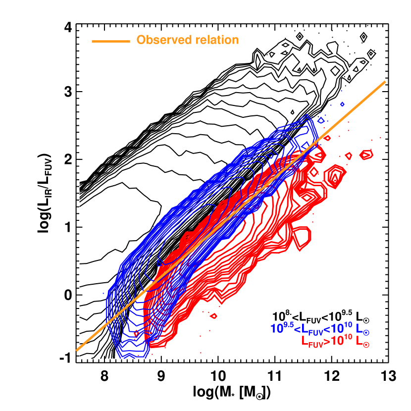
Figure 6: Simulated FIR to UV luminosity ratio as a function of stellar mass from a mock catalogue (see text). The red ($L_{\rm FUV}>10^{10}\,\rm{L}_{\odot}$) and blue ($10^{9.5}<L_{\rm FUV}/\rm{L}_{\odot}<10^{10}$) contours show mock galaxies within the same range of $L_{\rm FUV}$ as we probe in the data. The black ($10^{8.}<L_{\rm FUV}/\rm{L}_{\odot}<10^{9.5}$) contours show the mock galaxy distribution obtained through extrapolation of the UV luminosity function (see text). The solid line represents the observed relation, determined from galaxies with $L_{\rm FUV}>10^{9.5}\rm{L}_{\odot}$.

We investigate here the impact of the faint UV population on the recovery of the relation between dust attenuation and stellar mass. We follow the approach of Reddy et al. (2012b) to create a mock catalogue, which has the following properties: $L_{\rm FUV}$, $L_{\rm IR}$, SFR, and $M_{*}$. Our goal here is to model the intrinsic relation between dust attenuation and stellar mass, by taking into account galaxies fainter than the detection limit.

We focus here on the $z\sim 1.5$ case, but show in Appendix C results for $z\sim 3$ and $z\sim 4$. In practice, we consider the best fit of the UV luminosity function at $z\sim 1.5$ we determined for our sample (Heinis et al., 2013), down to $L_{\rm FUV}=10^{8}\rm{L}_{\odot}$. We build a mock catalogue by assigning UV luminosities according to this luminosity function. Then we assign a FIR luminosity to each object of this catalogue. We assume that the distribution of $\log(L_{\rm IR}/L_{\rm FUV})$ is a Gaussian. We use as mean of this distribution the stacking results from Heinis et al. (2013), and as dispersion, the dispersion required to reproduce the few per cents of UV-selected objects detected at SPIRE wavelength. We only have measurements for objects brighter that $L_{\rm FUV}=10^{9.5}\rm{L_{\odot}}$. For fainter objects, we assume that $\log(L_{\rm IR}/L_{\rm FUV})$ is constant, as well as its dispersion, using the results from Heinis et al. (2013). The values of these constants are $\log(L_{\rm IR}/L_{\rm FUV})_{\mathrm{faint}}=0.94$, and $\sigma(\log(L_{\rm IR}/L_{\rm FUV}))_{\mathrm{faint}}=0.73$. The value $\log(L_{\rm IR}/L_{\rm FUV})_{\mathrm{faint}}$ is higher than the average value for the sample $\langle\log(L_{\rm IR}/L_{\rm FUV})\rangle=0.84\pm 0.06$, but consistent with the values measured at the faint end of the sample. We determined this value in Heinis et al. (2013) such that the IR luminosity function of a UV selection recovers the IR luminosity function of a IR selection. Given the limited constraints on the latter, the assumption that $\log(L_{\rm IR}/L_{\rm FUV})$ and its dispersion are constant for $L_{\mathrm{FUV}}$ fainter that the limit of our sample is necessary. The conclusions we draw from this modeling exercise would differ if the average IR to UV luminosity ratio for galaxies fainter than the limit of our sample is similar to that of the galaxies of the sample, which is unlikely given the available data.

Having now a mock catalogue with $L_{\rm FUV}$ and $L_{\rm IR}$, we can assign a SFR to each of the objects by adding the IR and UV contributions. We finally assign a stellar mass by assuming the average SFR-mass relation we observe at $z\sim 1.5$, and assuming a dispersion of 0.15 dex (Béthermin et al., 2012). Note that this value might underestimate the actual dispersion of the SFR-mass relation, but this does not have a strong impact on our results here. We also checked that there is no impact of incompleteness in UV on the SFR-mass relation we observe (see Appendix B).

We show in Fig. 6 our modeled intrinsic IR to UV luminosity ratio as a function of stellar mass and per bins of $L_{\rm FUV}$from this mock catalogue. Note that we attempt to model the intrinsinc distribution, but that our mock catalogue is also self-consistent as we recover the observed dust attenuation-stellar mass relation for galaxies with $L_{\rm FUV}>10^{9.5}\,\textrm{L}_{\odot}$. The results from Fig. 6 show that fainter objects in UV have smaller stellar masses and higher dust attenuation. Our mock catalogue suggests that we observe a relation between the IR to UV luminosity ratio and $M_{*}$ partly because we are probing a limited range of $L_{\rm FUV}$. We note also that we observe that the dispersion in dust attenuation is larger for fainter galaxies (see Heinis et al., 2013, and also Fig. 4). Our mock catalogue shows that this dispersion actually originates from the $L_{\rm IR}/L_{\rm FUV}-M_{*}$ relation.

Our previous results also suggest that galaxies fainter than the current sensitivity levels in UV restframe luminosity (i.e. down to $u^{*}\sim 30$) are dustier. If that is the case, this suggests then that the actual average relation between $L_{\rm IR}/L_{\rm FUV}$ and stellar mass has a higher amplitude than the one we are observing, and also that the actual dispersion in dust attenuation at a given stellar mass is much higher, because of faint UV galaxies.

5 Discussion

5.1 Impact of UV-selection on SFR-Mass relations

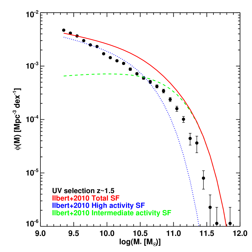
Figure 7: Mass function of the $z\sim 1.5$ UV-selected sample (black circles), compared the mass functions of star-forming galaxies in a $3.6\,\mu m$ selected-sample (Ilbert et al., 2010). The dotted line shows the best-fit to the mass function of their high activity star forming galaxies, while the dashed line shows that of the intermediate activity star forming galaxies. The solid line shows the sum of these two mass functions, representing the total mass function of star-forming galaxies.

We derive here average SFR-$M_{*}$ relations for UV-selected samples from $z\sim 4$ to $z\sim 1.5$. While the relations we obtain are not strongly sensitive to incompleteness in the UV, our results are not drawn from a mass selection. We investigate here whether this has any impact on our results.

We note first that we derive SFR-$M_{*}$ relations which have slopes consistent with 0.7 from $z\sim 4$ to $z\sim 3$, which is shallower than the value of $\sim 1$ derived by a number of studies (Elbaz et al., 2007; Daddi et al., 2007; Magdis et al., 2010; Wuyts et al., 2011), but in agreement with Karim et al. (2011); Noeske et al. (2007); Oliver et al. (2010); Whitaker et al. (2012). This shallower slope might be caused by the fact that we are selecting galaxies by their UV flux, and hence missing objects which have low star formation rates. To further examine this, we compare in Fig. 7 the mass function of our sample at $z\sim 1.5$ with mass functions derived from a mass-selected sample (Ilbert et al., 2010), based on $3.6\,\mu$m data. This comparison shows that the mass function of our UV-selected sample is similar to the total mass function of star-forming galaxies only at the low mass end, and is otherwise lower. Ilbert et al. (2010) also divided their sample into high activity and intermediate activity star forming galaxies, based on the restframe $NUV-R$ color. Fig. 7 shows that the mass function of UV-selected galaxies at $z\sim 1.5$ is similar to that of high activity star-forming galaxies at $M_{*}<10^{10.5}\,\textrm{M}_{\odot}$, while it is larger above this mass. On the other hand, the mass function of UV-selected galaxies at $z\sim 1.5$ is lower than that of intermediate star-forming galaxies at $M_{*}>10^{10.5}\,\textrm{M}_{\odot}$.

This comparison suggests that the UV-selection at $z\sim 1.5$ is likely to probe the full population of highly star-forming galaxies, while it may miss roughly half the number density of intermediate star-forming ones at $M_{*}>10^{10.5}\,\textrm{M}_{\odot}$. We note that at $z\sim 3$ and $z\sim 4$ UV-selected samples also miss a significant fraction of high stellar mass galaxies. This shows that the amplitudes of our SFR-Mass relations might be overestimated, and also that there might be an impact on the slope of these relations, if these high stellar mass galaxies we are missing have high SFR and large dust attenuation.

On the other hand, we can also in this context compare our results to those from Karim et al. (2011), who perform radio stacking on a mass-selected sample. They derive SFR-mass relations which have an amplitude at most 2 times lower than ours, and a similar slope. Note that Karim et al. (2011) measure SFRs from stacking in VLA-radio data. While some contamination by AGN is possible, we consider here for the comparison their results from star-forming galaxies, which are not expected to be dominated by radio-AGNs (Hickox et al., 2009; Griffith & Stern, 2010).

5.2 Impact of star formation history on conversion from observed UV and IR luminosities to SFR

The values of the factors commonly used to convert from UV or IR luminosities to SFR (Kennicutt, 1998) assume that the star formation has been constant over timescales of around 100 Myrs. While useful, this assumption is not correct for galaxies with other star formation histories. The impact of the star formation history on the conversion from $L_{\rm FUV}$ or $L_{\rm IR}$ to SFR has been studied by various authors (including Kobayashi, Inoue, & Inoue, 2013; Reddy et al., 2012b; Schaerer, de Barros, & Sklias, 2013): in the early phases of star formation ($t<10\,$Myr), the actual conversion factors are larger than the Kennicutt (1998) values (implying that the SFR values are underestimated when adopting the conversion factor from Kennicutt (1998)), while for later phases there are lower. The amplitude of the difference depends on the star formation history, with faster evolutions yielding larger differences. In our case, if we assume that our SFR values are overestimated, this means that the bulk of our samples is a population of galaxies in later phases of star formation, with rapidly declining star formation histories, like starbursts for instance. It is beyond the scope of this paper to characterise precisely the star formation histories of the galaxies in our samples. We can however base our argumentation on the results of SED fitting of dropouts at $3<z<6$ from Schaerer, de Barros, & Sklias (2013). They found that the currently available data is suggesting that these galaxies experienced either exponentially declining or delayed star formation histories. They also note in particular that, assuming their SED fitting, the SFR would be slighty underestimated if the Kennicutt (1998) conversion factors would have been used. Moreover, Wuyts et al. (2011) showed by backtracing galaxies using different star formation histories that the declining star formation scenario does not enable to reproduce the number densities of star-forming galaxies between $z=4$ and $z=0$. In summary, given the state-of-the art SED fitting, we believe that the impact of star formation histories different from that assumed by Kennicutt (1998) is negligible on our results.

5.3 Evolution of specific star formation rate with redshift

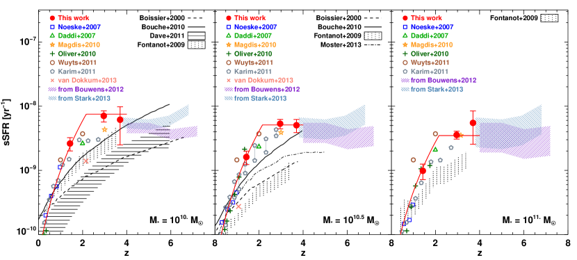
Figure 8: Specific star formation versus redshift for a stellar mass of $10^{10}\,\textrm{M}_{\odot}$ (left), $10^{10.5}\,\textrm{M}_{\odot}$ (middle), $10^{11}\,\textrm{M}_{\odot}$ (right). Our results are showed as red filled circles. The red thick line is a fit to our measures using eq. 5.4 (see Sect. 5.4). We compare our resuls to those of van Dokkum et al. (2013, crosses, for Milky Way-like galaxies), Noeske et al. (2007, open squares), Daddi et al. (2007, open triangle), Magdis et al. (2010, open star, shifted by $+0.15$ in redshift at $M_{*}=10^{11}\,\textrm{M}_{\odot}$ for clarity), Oliver et al. (2010, plus symbols), Wuyts et al. (2011, open circles), Karim et al. (2011, star forming sample, open pentagons), and to the range of values allowed by the results of Bouwens et al. (2012, diagonally hatched regions, see text for details); Stark et al. (2013, diagonally hatched regions, see text for details). At $M_{*}=10^{10.5}\,\textrm{M}_{\odot}$, for the values of Karim et al. (2011), we show their results at $M_{*}\sim 10^{10.37}\,\textrm{M}_{\odot}$ and $M_{*}\sim 10^{10.75}\,\textrm{M}_{\odot}$, as they do not list measurements at $M_{*}=10^{10.5}\,\textrm{M}_{\odot}$. We compare these observations to the models of Boissier & Prantzos (2000, dashed line), Bouché et al. (2010, solid line), Davé, Oppenheimer, & Finlator (2011, horizontally hatched regions), Fontanot et al. (2009, vertically hatched regions) and Moster, Naab, & White (2013, dot dashed line).

Our measurements show that the amplitude of the SFR-$M_{*}$ relation is similar between $z\sim 4$ and $z\sim 3$, and then decreases significantly from $z\sim 3$ to $z\sim 1.5$. Another way to look at these results is to consider the specific star formation rate $\rm{sSFR}=\rm{SFR}/M_{*}$ which is an indicator of star formation history, in the sense that it is the inverse of the time needed for a galaxy to double its mass if it has a constant SFR.

We show in Fig. 8 the evolution with redshift of the specific star formation rate for three mass bins: $10^{10}\,\textrm{M}_{\odot}$, $10^{10.5}\,\textrm{M}_{\odot}$, and $10^{11}\,\textrm{M}_{\odot}$. We compute the average SFR for our samples by stacking galaxies in bins of stellar mass centered on these values, with sizes of 0.2 dex at $z\sim 1.5$ and $z\sim 3$, and a size of 0.4 dex at $z\sim 4$.

We compare our results to the measurements of Daddi et al. (2007); van Dokkum et al. (2013); Karim et al. (2011); Magdis et al. (2010); Noeske et al. (2007); Wuyts et al. (2011). At $z>4$, there are basically no results yet in the mass range we explore. We show here an extrapolation of the results from Bouwens et al. (2012) and Stark et al. (2013). Bouwens et al. (2012) give values of sSFR at $M_{*}=5\times 10^{9}\,\textrm{M}_{\odot}$ corrected from dust attenuation (based on the UV slope of the continuum), using their own sample at $z=4$, and the results from Stark et al. (2009) and González et al. (2010) at higher redshifts. Stark et al. (2013) derive sSFRs also at $M_{*}=5\times 10^{9}\,\textrm{M}_{\odot}$ at $4<z<7$, taking into account the impact of emission lines on the measure of stellar masses, and correcting from dust attenuation using the slope of the UV continuum. We extrapolate results from both studies in our mass range assuming that there is a power law relation between SFR and stellar mass at $z>4$, and that the slope of this relation is between 0.7 (the value measured at $z=4$ by Bouwens et al. (2012), also consistent with our results) and 1 (closer to the value observed at lower redshifts by other studies like Wuyts et al., 2011).

Our results are in overall agreement with previous measurements at $z\sim 1.5$. Note that all measurements are significantly higher than those of van Dokkum et al. (2013), who derived the star formation history of Milky Way-like galaxies (see Sect. 5.4 for further discussion).

At $z\sim 3$, our measurements are quite high compared to the values from previous studies, in particular at $M_{*}=10^{10}\,\textrm{M}_{\odot}$. In this mass bin, our estimates are larger than the measurements from Karim et al. (2011) and Magdis et al. (2010), but they are consistent at $1.2\,\sigma$ and $0.3\,\sigma$ respectively. In other word, our sSFR results represent the upper range of available measurements. Note however that our results are in very good agreement with those of Magdis et al. (2010) at $z\sim 3$ for $M_{*}=10^{10.5.}\,\textrm{M}_{\odot}$ and $M_{*}=10^{11.}\,\textrm{M}_{\odot}$.

At $z\sim 4$, our results agree with those from Bouwens et al. (2012) and Stark et al. (2013) at $z=4$. Our results are also in agreement with the sSFR being constant at $3<z<4$, while the results of Stark et al. (2013) suggest that the sSFR is increasing at higher redshifts ($z>5$).

We compare our results with a few models, from Boissier & Prantzos (2000), Bouché et al. (2010), Davé, Oppenheimer, & Finlator (2011), Fontanot et al. (2009), and Moster, Naab, & White (2013). These models are quite different and give a sample of various simulation techniques available. We briefly describe all of them.

Boissier & Prantzos (2000, see also () and ()) built an analytical model which predicts the chemical and spectrophotometric evolution of spiral galaxies over the Hubble time. This model reproduces a large number of present properties of the Milky Way and local spiral galaxies (such as: color-magnitude diagrams, luminosity-metallicity relationship, gas fractions, as well as color and metallicity gradients). Bouché et al. (2010) based their model under the assumption that the gas accretion in galaxies is mostly driven by the growth of dark matter haloes (e.g. Dekel et al., 2009). They also assume that the gas accretion efficiency decreases with cosmic time, and is only efficient for dark matter haloes of masses $10^{11}<M_{h}/\textrm{M}_{\odot}<1.5\times 10^{12}$. Davé, Oppenheimer, & Finlator (2011) ran hydrodynamical simulations which include galactic outflows, implementing several models for winds; we show on Fig. 8 the range of sSFR spanned by these models, including the model without winds. Fontanot et al. (2009) compared the predictions from three semi-analytical models, namely those of De Lucia & Blaizot (2007); Monaco, Fontanot, & Taffoni (2007); Somerville et al. (2008). All three models are based on the combination of dark matter simulations complemented by empirical relations for baryonic physics. All these models include supernovae and AGN feedback. We show on Fig. 8 the range of sSFR spanned by these three models. Moster, Naab, & White (2013) studied the mass assembly of galaxies using abundance matching models, by matching observed stellar mass functions simultaneously at various redshifts.

The comparison in Fig. 8 of observations and models shows that models match the observations roughly well at low redshift ($z<0.5$, see also e.g. Damen et al., 2009), underestimate the sSFR up to $z=4$, and are potentially in better agreement at higher redshifts. An interesting point is that the models we consider here are quite different in terms of implementation and assumptions; however they all predict a similar evolution which does not match the observations for $0.5\la z\la 4$. At $M_{*}=10^{10}\textrm{M}_{\odot}$, the model of Bouché et al. (2010) and the compilation of models from Fontanot et al. (2009) are the closest to the observations among the ones we consider here. Still, these models do not reproduce the high sSFR we observe at $z\sim 3$. At $M_{*}=10^{10.5}\textrm{M}_{\odot}$, the model of Bouché et al. (2010) presents the same level of agreement with our measurements, while the discrepancies between the compilation of Fontanot et al. (2009) and the observations are more important. We note also that all these models are actually more or less consistent with the redshift evolution expected according to the cold gas accretion scenario (Dekel et al., 2009). This scenario predicts that the baryonic accretion onto galaxies follows directly the dark matter accretion onto dark matter haloes, and evolves as $\dot{M}\propto(1+z)^{2.25}$. Our results show that this scenario is in agreement with the observations for $0<z\la 1.5$, but is less efficient at reproducing galaxies properties at $1.5\la z\la 3$.

There has been some attempts to reconcile model predictions with the observations of the redshift evolution of the sSFR. Davé (2008) noted that a number of observations suggest that the IMF is not universal and could evolve with redshift, in the sense that it would be weighted towards more massive stars at high redshift. Such an IMF would imply that SFRs as derived here are overestimated with respect to using an evolving IMF, by a factor that increases with redshift, being around 4 at $z=4$. Whether the IMF is universal, or evolves with redshift, remains to date a controversial subject. Indeed recent studies suggest in contrary to Davé (2008) that there is observational evidence for bottom-heavy IMF at high redshift (see e.g. van Dokkum & Conroy, 2012).

Weinmann, Neistein, & Dekel (2011) considered a number of modifications to semi-analytical models in order to match the observed redshift evolution of the sSFR. They found that models can match the observations at $z>4$ if there is either strong stellar feedback at high redshift at all masses, or inefficient star formation. At $z=2-3$, where the models underpredict the sSFR, the feedback could drop, or gas which was prevented to form stars earlier could be at that time available for star formation. We provide new and improved observational constraints to test these scenarios. Future observations of the gas content of high redshift galaxies will also enable to discriminate between those.

5.4 The star formation histories of Main sequence galaxies

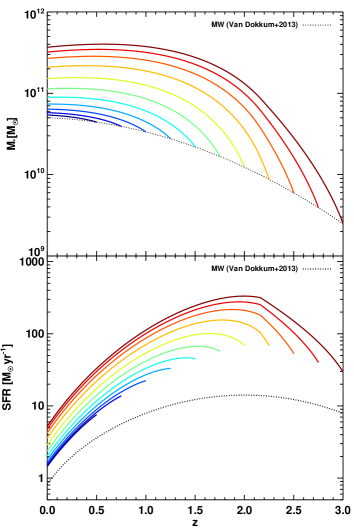
Figure 9: Star formation history of Main Sequence galaxies which have the same stellar mass as the Milky Way. We integrate here the sSFR of the Main Sequence; we use the best fit to our measurements of $\mathrm{sSFR_{\mathrm{MS}}}(z,M_{*})$ (eq. 5.4). Top: evolution of the stellar mass for Main Sequence galaxies, assuming that galaxies have the same stellar mass as the Milky Way at 10 equally spaced redshifts values ranging from $z=3$ to $z=0.5$ according to the measurements of van Dokkum et al. (2013) (dotted line); the redshifts are color-coded: bluer for lower initial redshift for the integration boundary condition. Bottom: Same as top plot, but for the star formation rate, with corresponding colors.

Our measurements bring new constraints at high redshift on the sSFR of the Main Sequence galaxies. We can use these results to derive the star formation history of galaxies staying on the Main Sequence. We first recall that galaxies can not remain on the Main Sequence from high redshift to $z=0$, given the stellar masses and SFR they would have in the local Universe. We then give estimates of the timescale galaxies can stay on the Main Sequence before quenching of the star formation.

We consider here a parameterised form of the dependence with redshift and stellar mass of the sSFR of the Main Sequence. We follow the approach of Béthermin et al. (2012), and we assume that:

$$\mathrm{sSFR}_{\mathrm{MS}}(z,M_{*}) = \mathrm{sSFR_{\mathrm{MS,0}}}\times\left(\frac{M_{*}}{10^{11}\,\textrm{M}_{\odot}}\right)^{\beta_{\mathrm{MS}}}$$

$$\times\left(1+\min(z,z_{\rm evo})\right)^{\gamma_{\mathrm{MS}}}\mathrm{,}$$

where $\mathrm{sSFR_{\mathrm{MS,0}}}$ is the sSFR of the Main Sequence at $z=0$ for galaxies of $M_{*}=10^{11}\textrm{M}_{\odot}$, $\beta_{\mathrm{MS}}$ is the slope of the sSFR-$M_{*}$ relation, and $\gamma_{\mathrm{MS}}$ encodes the power-law redshift evolution of the amplitude of the sSFR-$M_{*}$ relation. We modify the values of these parameters to match our measurements as well as the measurements at lower redshifts from Noeske et al. (2007): $\mathrm{sSFR}_{\mathrm{MS,0}}=10^{-10.66}\mathrm{yr}^{-1}$, $\beta_{\rm MS}=-0.33$, $z_{\rm evo}=2.16$, and $\gamma_{\rm MS}=4.4$. We show the resulting sSFR evolution using these parameters as a red line on Fig. 8.

We note that eq. 5.4 can also be written as

$$\frac{1}{1-R}\frac{1}{M_{*}}\frac{\mathrm{d}M_{*}}{\mathrm{d}t} = \mathrm{sSFR_{MS,0}}\times\left(\frac{M_{*}}{10^{11}\,\textrm{M}_{\odot}}\right)^{\beta_{\rm MS}}$$

$$\times\left(1+\min\left(z(t),z(t_{\rm evo})\right)\right)^{\gamma_{\rm MS}}$$

where $t_{\rm evo}$ is the lookback time corresponding to $z_{\rm evo}$. We wrote the SFR in terms of the derivative of $M_{*}$ with respect to time assuming that

$$\frac{\mathrm{d}M_{*}}{\mathrm{d}t}=\mathrm{SFR}(1-R)\mathrm{.}$$ (9)

$R$ is the return fraction, that we set to (Conroy & Wechsler, 2009)

$$R=0.05\ln\left(1+\frac{\Delta t}{0.03\mathrm{Myr}}\right)$$ (10)

where $\Delta t$ is the time elapsed since the formation of stars.

We can then use the fact that eq. 5.4 is a differential equation for $M_{*}(z)$. We obtain $M_{*}(z)$, and from this SFR$(z)$. This procedure requires boundary conditions of stellar mass at a given redshift. In other words, we can start the integration of eq. 5.4 at any redshift, but we need to choose an initial stellar mass at this redshift. This means that we are making galaxies ’enter’ on the Main Sequence at these stellar mass and redshift. We are considering here only the mean location of the Main Sequence. This means that, prior to entering the Main Sequence in the sense of this simple model, galaxies could for instance be lower in the SFR-Mass plane, but still within the Main sequence at redshifts higher than this initial redshift.

We consider here the result of van Dokkum et al. (2013), who derive the star formation history of Milky Way-like galaxies, by studying up to $z=2.5$ galaxies with the same number density as galaxies with the stellar mass of Milky Way at $z=0$. van Dokkum et al. (2013) derive the redshift evolution of the stellar mass of such galaxies. We use their fit to get initial stellar mass at a given redshift.

We integrate eq. 5.4 down to $z=0$, starting from various initial redshifts, which we consider between $z=3$ and $z=0.5$. We show on Fig. 9 the evolution of the stellar mass and SFR for galaxies which remain on the Main Sequence and have the same stellar mass as the Milky Way at these initial redshifts. Doing so we look at the star formation history of galaxies which have the same stellar mass as the Milky Way at these initial redshifts, and stay on the Main Sequence until $z=0$.

Assuming that a galaxy is on the Main Sequence for $1\la z<3$ leads to much higher SFR and stellar mass than the Milky Way at $z=0$. On the other hand, if we assume that the Milky Way is on the Main Sequence between $z=0.5$ and $z=0$, we obtain a stellar mass similar to the Milky Way at $z=0$, and a SFR around 2 times higher. Note that galaxies with $M_{*}\sim 10^{10}\,\textrm{M}_{\odot}$ at $z\sim 2$ would have $M_{*}\sim 2\times 10^{11}\,\textrm{M}_{\odot}$ at $z=0$. This is in strong disagreement with measurements of the redshift evolution of the stellar mass functions of star forming galaxies (e.g. Ilbert et al., 2010) which show little evolution between $z=2$ and $z=0$ at the high mass end. The star formation histories on Fig. 9 are actually quite different from that expected for the Milky Way (dotted line on bottom panel), even though we assumed the observed stellar mass of Milky Way-like galaxies at various redshifts as boundary conditions. This is actually due to the fact that the Milky Way is not on the mean location of the Main Sequence for $1<z<2$ (see crosses showing the measurements of van Dokkum et al. (2013) on Fig. 8). Assuming the values from van Dokkum et al. (2013) and the results of Wuyts et al. (2011) for the distribution of galaxies in the $(\mathrm{SFR},M_{*})$ plane suggests that the Milky Way is rather on the lower enveloppe of the Main Sequence for $0<z<2$. Our results suggest on the other hand that the sSFR of star-forming galaxies is quite high at $z=3,4$, which yields a high SFR peak in the derived star formation histories.

The results shown on Fig. 9 suggests that the assumption that galaxies remain on the Main Sequence until $z=0$ is not correct. The consequence is that the Main Sequence is built of different star-forming galaxies at various redshifts.

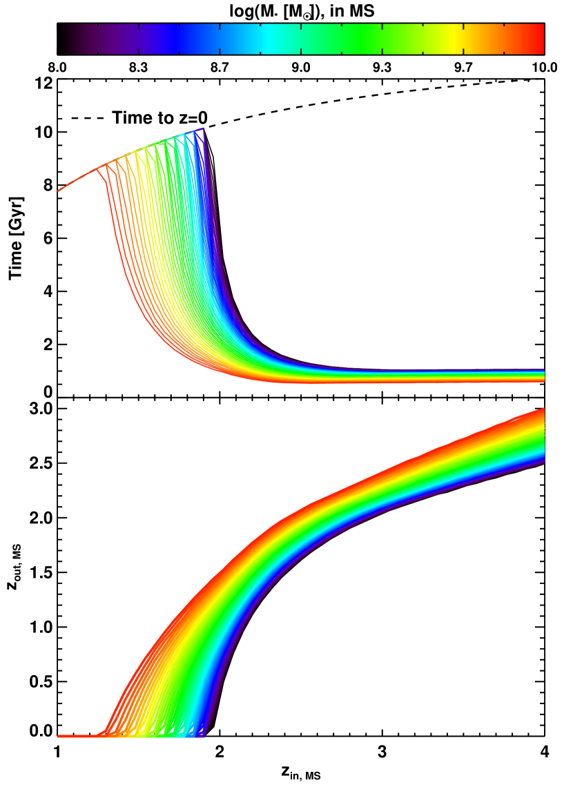
Figure 10: Top: time galaxies stay on the Main Sequence before quenching of star formation, as a function of the redshift they enter on the Main Sequence. The dashed line shows the time left until $z=0$. Bottom: redshift of galaxies when they exit the Main Sequence, as a function of the redshift they enter on the Main Sequence. In both plots, the color codes the stellar mass of galaxies at the time they enter on the Main Sequence, ranging from $10^{8}$ to $10^{10}\,\textrm{M}_{\odot}$.

These results raise the question of the amount of time galaxies can stay on the Main Sequence. In order to determine this time, we need to define a criterion to determine the epoch when galaxies exit the Main Sequence. We use here the ‘quenching mass’ ($M_{\rm Q}$) as defined by Ilbert et al. (2013). We used the same method as above to investigate this. We consider once again eq. 5.4, but this time we stop the integration, i.e. we make galaxies exit the Main Sequence, at the redshift when their stellar mass is larger than the quenching mass at the same time. Galaxies experiencing quenching of star formation exit the Main Sequence by going down in the $(\mathrm{SFR},M_{*})$ plane at a given M_∗ (e.g. Wuyts et al., 2011). We do not consider here starbursts galaxies as they represent a significantly smaller number density (Rodighiero et al., 2011).

We follow Ilbert et al. (2013) and assume that the quenching mass is the mass where the number density of quiescent galaxies is maximum. We consider the measurements from Ilbert et al. (2013) of the mass function of quiescent galaxies (available for $0.5<z<3$) and complement them at $z=0$ by the measurement of Baldry et al. (2012). The evolution with redshift of the quenching mass can be adjusted to the following form:

$$M_{\rm Q}(z)[\textrm{M}_{\odot}]=3.7\times 10^{10}\times(1+z)^{0.53}$$ (11)

We make the galaxies enter the Main Sequence at redshifts $1<z<4$, and at masses in the range $10^{8}<M_{*}/\textrm{M}_{\odot}<10^{10}$. We show the time galaxies stay on the Main Sequence in Fig. 10. We perform the integration only until $z=0$; in other words, we do not derive times larger than the time to $z=0$ for galaxies that have not reached $M_{\rm Q}$ at $z=0$. This means that galaxies that are still on the Main Sequence at $z=0$ are represented by locations on the dashed line on the top panel of Fig. 10, or at $z=0$ in the bottom panel.

Given our assumptions, our results show that galaxies which enter the Main Sequence at $z<4$ stay on it at least 1 Gyr. As expected, at a given entrance redshift on the Main Sequence, less massive galaxies spend more time on the Main Sequence to reach the quenching mass. Galaxies entering on the Main Sequence at $2.5<z<4$ stay around 1 Gyr on it. At lower redshifts, the quenching mass decreases, but the average sSFR also decreases, which in turn yields that galaxies stay longer on the Main Sequence. For instance, with the scenario we consider here, galaxies with masses $10^{8}<M_{*}/\textrm{M}_{\odot}<10^{10}$ which enter the Main Sequence at $z<1.2$ stay on the Main Sequence until $z=0$. Leitner (2012) and Zahid et al. (2012) reach similar conclusions regarding the star formation histories of Main Sequence galaxies at $z<2$.

We assumed here that the sSFR is constant for $z>2.16$. Assuming that the sSFR increases with $z$ from $z\sim 3$ (see e.g. Stark et al., 2013) would mean faster evolution for high redshift galaxies, implying: stronger disagreement for the evolution of the Milky Way as discussed here, and shorter times on the Main sequence for high redshift galaxies. We note that the simplistic calculation presented here requires to be tested against the redshift evolution of the stellar mass functions of quiescent and star forming galaxies, which is beyond the scope of this paper, and will be the subject of forthcoming work.

6 Conclusions

We studied the FIR properties of large samples of UV-selected galaxies at $1.5<z<4$, by combining the COSMOS multiwavelength dataset with the HerMES/Herschel SPIRE imaging. We measured by stacking the average IR luminosity as a function of UV luminosity, stellar mass, and both. Our results can be summarised as follows:

1. [1.]

2. At $z\sim 1.5$, there is a good correlation between $L_{\rm IR}$ and $L_{\rm FUV}$($8\times 10^{9}<L_{\rm FUV}/L_{\odot}<5\times 10^{10}$), while at $z\sim 3$ and $z\sim 4$, $L_{\rm IR}$ and $L_{\rm FUV}$ are not well correlated.

3. Consequently, the ratio $L_{\rm IR}$ $/$$L_{\rm FUV}$ at $z\sim 3,4$ is decreasing with $L_{\rm FUV}$.

4. The average dust attenuation (as traced by the $L_{\rm IR}$ $/$$L_{\rm FUV}$ ratio) is well correlated with stellar mass at $1.5<z<4$, and does not show significant evolution in this redshift range, in the range of masses we explore.

5. We investigated the joint dependence of dust attenuation with stellar mass and $L_{\rm FUV}$. While well correlated with stellar mass, dust attenuation also shows secondary dependence on $L_{\rm FUV}$. At a given stellar mass, dust attenuation decreases with $L_{\rm FUV}$; at a given $L_{\rm FUV}$, dust attenuation increases with stellar mass. We also provide empirical relations between dust attenuation, $M_{*}$, and $L_{\rm FUV}$, at $z\sim 1.5$ and $z\sim 3$.

6. The average SFR-$M_{*}$ relations for UV-selected samples at $1.5<z<4$ are well approximated by a power law, with a slope of around 0.7. At a given stellar mass, the average SFR is similar at $z\sim 3$ and $z\sim 4$, but is 4 times higher than at $z\sim 1.5$.

7. Our results provide new constraints on the sSFR at $1.5<z<4$. Current models of galaxy formation and evolution do not reproduce accurately the sSFR evolution we observe, in particular at $z\sim 3$ and $z\sim 4$, where standard models underpredict the observations.

8. We use our results for the evolution of the sSFR with redshift to characterise the star formation histories of Main Sequence galaxies. We find that galaxies would have too large stellar masses if they stay on the Main Sequence from high redshift to $z=0$. Assuming that galaxies exit the Main Sequence when their stellar mass is equal to the ‘quenching mass’, we determine the time galaxies stay on the Main Sequence. This suggests that galaxies stay around 1 Gyr on the Main Sequence at high redshift ($2.5<z<4$), while they stay longer on the Main Sequence at lower redshifts. For instance, Main Sequence galaxies (with $10^{8}<M_{*}/\textrm{M}_{\odot}<10^{10}$) at $z=1$ stay until $z=0$ on the Main Sequence, as they do not reach the quenching mass.

Appendix A Empirical recipes for dust attenuation correction

We provide here empirical relations to correct for dust attenuation, given observed UV luminosity and stellar mass. We show the relations between the infrared to UV luminosity ratio and the stellar mass, for several bins of UV luminosity, at $z\sim 1.5$ (Fig. 11) and at $z\sim 3$ (Fig. 12). These measurements are the same as those presented in Fig. 4. We assume that

$$\mathrm{IRX}(L_{\rm FUV},M_{*})=\mathrm{IRX_{0}}(L_{\rm FUV})+\delta(L_{\rm FUV})\log\left(\frac{M_{*}}{10^{10.35}}\right)$$ (12)

where we set here $\delta(L_{FUV})=0.72$, which is the slope of the IRX$-M_{*}$ correlation for the full sample at $z\sim 1.5$, and is also valid at $z\sim 3$. We provide the best fit values for IRX${}_{0}(L_{\rm FUV})$ in Table 3 for $z\sim 1.5$ measurements and in Table 4 for $z\sim 3$ measurements. We include only the stacking measurements with $S/N>3$ in the fit, but including other stacking measurements does not have an impact on the results.

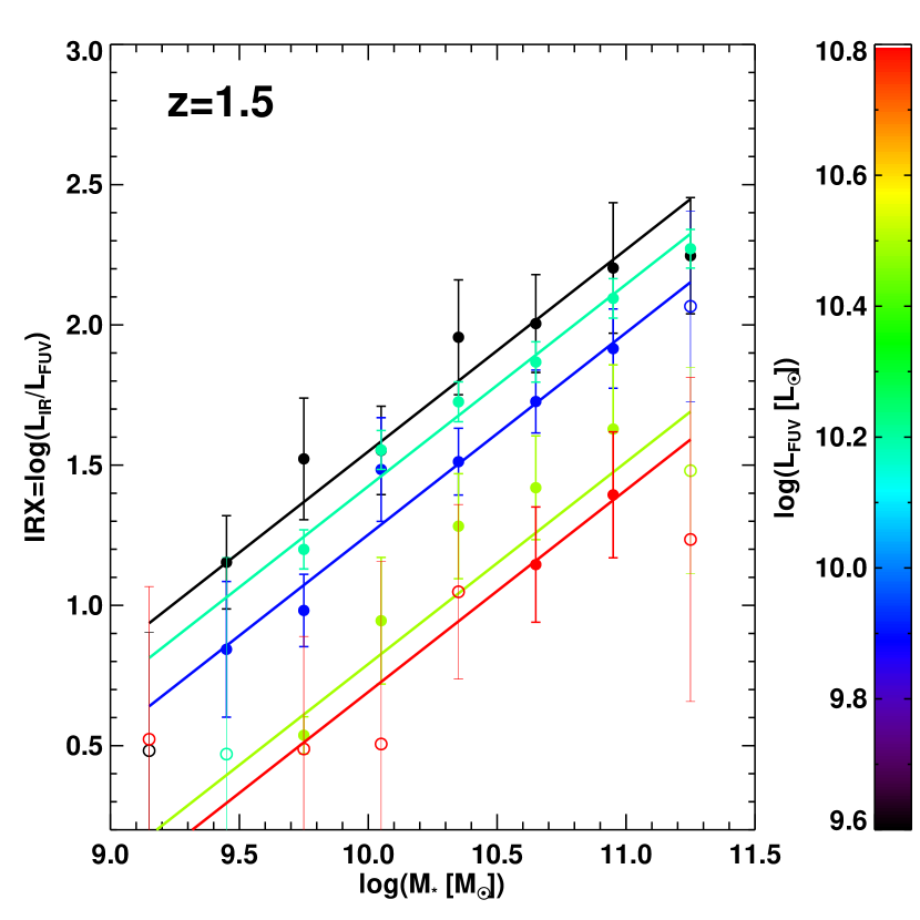
Figure 11: Infrared to UV luminosity ratio as a function of stellar mass, at $z\sim 1.5$. We show here the results from Fig. 4 along with fits by power laws. The mean UV luminosity is color-coded. Filled symbols represent stacking measurements with $S/N>3$ in all SPIRE bands, and open symbols other stacking measurements.

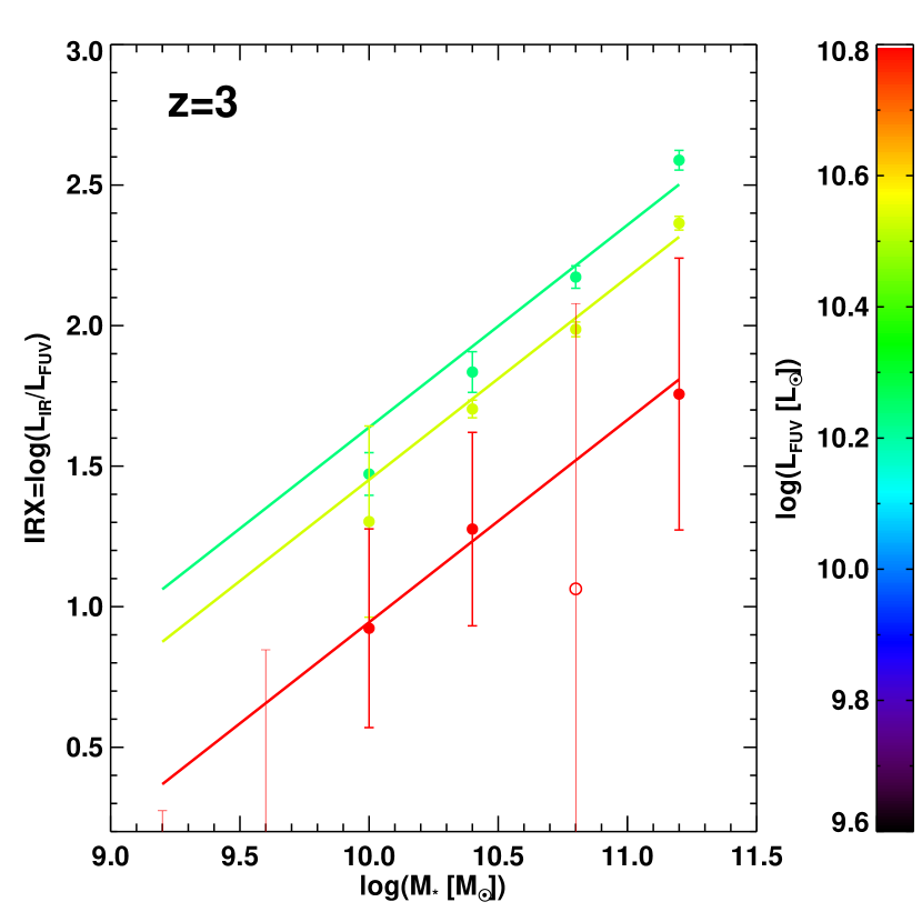
Figure 12: Same as Fig. 11, for the $z\sim 3$ sample.

Table 3: $z\sim 1.5$ best fit of IRX$-M_{*}-L_{\rm FUV}$ relation for stacking measures with $S/N>3$ in all SPIRE bands

$\log(L_{\rm FUV}[L_{\odot}])$ range	IRX0
9.44 – 9.74	1.80 $\pm$ 0.07
9.74 – 10.04	1.50 $\pm$ 0.06
10.04 – 10.34	1.68 $\pm$ 0.03
10.34 – 10.64	1.04 $\pm$ 0.05
10.64 – 10.94	0.94 $\pm$ 0.15

Table 4: $z\sim 3$ best fit of IRX$-M_{*}-L_{\rm FUV}$ relation for stacking measures with $S/N>3$ in all SPIRE bands

$\log(L_{\rm FUV}[L_{\odot}])$ range	IRX0
10.09 – 10.39	1.89 $\pm$ 0.02
10.39 – 10.69	1.70 $\pm$ 0.01
10.69 – 10.99	1.20 $\pm$ 0.21

Appendix B Impact of UV incompleteness on SFR-Mass relation

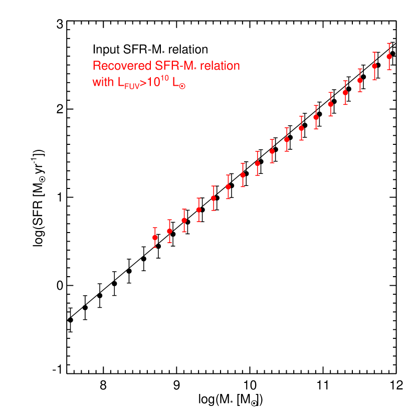
Figure 13: Simulated SFR-Mass relation at $z\sim 1.5$ from a mock catalogue. The black circles show the input SFR-Mass relation, and the red circles the recovered relation for galaxies brighter than $L_{\rm FUV}=10^{10}\,L_{\odot}$. Error bars represent the standard deviation.

We show here the impact of the incompleteness in $L_{\rm FUV}$ on the recovered SFR stellar mass relation. We use the same method as Reddy et al. (2012b) as described in Sect. 4.5 to create a mock catalogue. We show in Fig. 13 as black circles the input SFR-Mass relation at $z\sim 1.5$ from the mock catalogue we build. Red circles show the recovered SFR-Mass relation we obtain from this mock catalogue if we use only objects brighter than $L_{\rm FUV}>10^{10}\,L_{\odot}$. This shows that there is no impact of UV incompleteness on the SFR-Mass relation we observe.

Appendix C Bias on the estimation of dust attenuation relations at $z\sim 3,4$

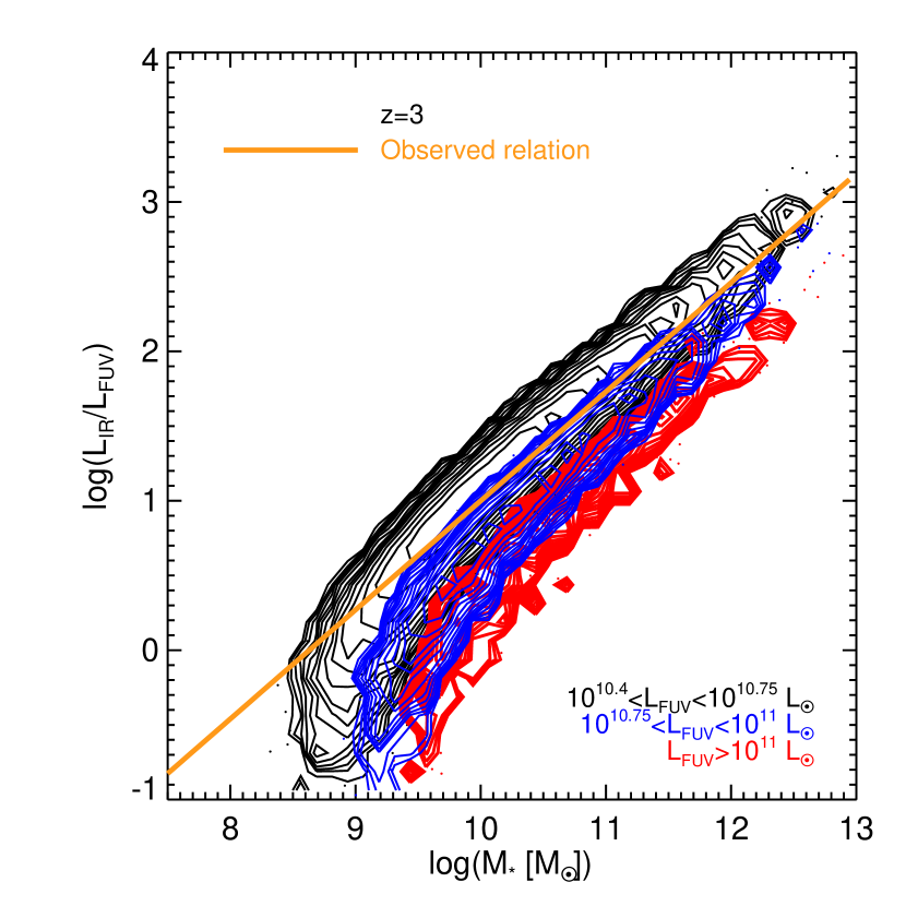
Figure 14: Simulated FIR to UV luminosity ratio as a function of stellar mass from a mock catalogue (see text) at $z\sim 3$. The red contours show mock galaxies with $L_{\rm FUV}>10^{11}\,\rm{L}_{\odot}$, blue contours galaxies with $10^{10.75}<L_{\rm FUV}/\rm{L}_{\odot}<10^{11}$, and black contours galaxies with $10^{10.4}<L_{\rm FUV}/\rm{L}_{\odot}<10^{10.75}$.The solid line represents the observed relation.

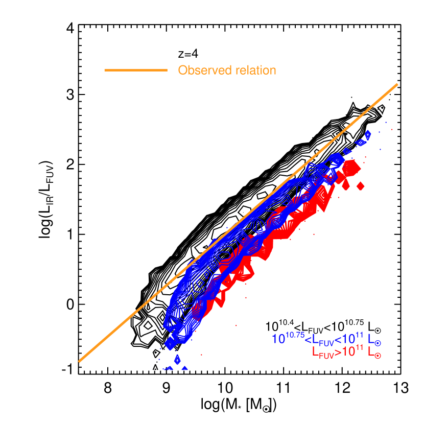
Figure 15: Simulated FIR to UV luminosity ratio as a function of stellar mass from a mock catalogue (see text) at $z\sim 4$. The red contours show mock galaxies with $L_{\rm FUV}>10^{11}\,\rm{L}_{\odot}$, blue contours galaxies with $10^{10.75}<L_{\rm FUV}/\rm{L}_{\odot}<10^{11}$, and black contours galaxies with $10^{10.4}<L_{\rm FUV}/\rm{L}_{\odot}<10^{10.75}$.The solid line represents the observed relation.

We show here the IR to UV luminosity ratio as a function of stellar mass from mock catalogues built as described in Sect. 4.5 at $z\sim 3$ in Fig. 14, and at $z\sim 4$ in Fig. 15. Note that here we do not extrapolate to UV luminosities fainter than the completeness limit of the samples as we do in Fig. 6.

References

- Arnouts et al. (2013) Arnouts S., et al., 2013, arXiv, arXiv:1309.0008
- Baldry et al. (2012) Baldry I. K., et al., 2012, MNRAS, 421, 621
- Bavouzet (2008) Bavouzet N., 2008b, PhD thesis, Université Paris-Sud XI, http://tel.archives-ouvertes.fr/docs/00/36/39/75/PDF/these_nb.pdf
- Béthermin et al. (2010) Béthermin M., Dole H., Beelen A., Aussel H., 2010, A&A, 512, A78
- Béthermin et al. (2011) Béthermin M., Dole H., Lagache G., Le Borgne D., Penin A., 2011, A&A, 529, A4
- Béthermin et al. (2012) Béthermin M., et al., 2012, ApJ, 757, L23
- Boissier & Prantzos (1999) Boissier S., Prantzos N., 1999, MNRAS, 307, 857