On the block maxima method in extreme value theory: PWM estimators
Ana Ferreiralabel=e1]anafh@isa.utl.pt
[Laurens de Haanlabel=e2]ldehaan@ese.eur.nl
[
ISA
Department of Economics
University of Lisbon
Tapada da Ajuda 1349-017 Lisboa
Portugal
and
CEAUL
FCUL
Bloco C6 - Piso 4 Campo Grande
749-016 Lisboa
Portugal
Department of Mathematics
Erasmus University Rotterdam
P.O. Box 1738
3000 DR Rotterdam
The Netherlands
and
CEAUL
FCUL
Bloco C6 - Piso 4 Campo Grande
749-016 Lisboa
Portugal
University of Lisbon and Erasmus Univ Rotterdam
(2015; 4 2014; 8 2014)
Abstract
In extreme value theory, there are two fundamental approaches, both
widely used: the block maxima (BM) method and the peaks-over-threshold
(POT) method. Whereas much theoretical research has gone into the POT
method, the BM method has not been studied thoroughly. The present
paper aims at providing conditions under which the BM method can be
justified. We also provide a theoretical comparative study of the
methods, which is in general consistent with the vast literature on
comparing the methods all based on simulated data and fully parametric
models. The results indicate that the BM method is a rather efficient
method under usual practical conditions.
In this paper, we restrict attention to the i.i.d. case and focus on
the probability weighted moment (PWM) estimators of
Hosking, Wallis and Wood [Technometrics (1985) 27 251–261].
62G32,
62G20,
62G30,
Block maxima,
peaks-over-threshold,
probability weighted moment estimators,
extreme value index,
asymptotic normality,
extreme quantile estimation,
doi:
10.1214/14-AOS1280
keywords:
[class=AMS]
keywords:
††volume: 43††issue: 1
\docsubty
FLA
T1Supported in part by FCT Project PTDC /MAT /112770 /2009;
EXPL/MAT-STA/0622/2013 and PEst-OE/MAT/UI0006/2014.
and
1 Introduction
The block maxima (BM) approach in extreme value theory (EVT),
consists of dividing the observation period into nonoverlapping
periods of equal size and restricts attention to the maximum
observation in each period [see, e.g., Gumbel (1958)]. The new
observations thus created follow—under domain of attraction
conditions, cf. (2) below—approximately an extreme
value distribution, for some real . Parametric
statistical methods for the extreme value distributions are then
applied to those observations.
In the peaks-over-threshold (POT) approach in EVT, one selects
those of the initial observations that exceed a certain high threshold.
The probability distribution of those selected observations is
approximately a generalized Pareto distribution Pickands (1975).
In the case of the POT method, exact conditions under which the
statistical method is justified can be described by a second-order term
[see, e.g., Drees (1998) and de Haan and Ferreira (2006), Section 2.3].
In the case of block maxima, usually it is taken for granted that the
maxima follow very well an extreme value distribution. In this paper,
we take this misspecification into account by quantifying it in terms
of a second-order expansion; cf. Condition 2.1 below.
Since is not the exact distribution for those observations,
a bias may appear.
The POT method picks up all “relevant” high observations. The BM method
on the one hand misses some of these high observations and, on the
other hand, might retain some lower observations. Hence the POT seems
to make better use of the available information.
There are practical reasons for using the BM method:
•
The only available information may be block maxima, for example,
yearly maxima with long historical records or long range simulated data
sets Kharin et al. (2007).
•
The BM method may be preferable when the observations are not
exactly independent and identically distributed (i.i.d.). For example,
there may be a seasonal periodicity in case of yearly maxima or, there
may be short range dependence that plays a role within blocks but not
between blocks; cf. for example, Katz, Parlange and Naveau (2002) and
Madsen, Rasmussen and Rosbjerg (1997) for further discussion.
•
The BM method may be easier to apply since the block periods
appear naturally in many situations [Naveau et al. (2009),
van den Brink, Können and Opsteegh (2005),
de Valk (1993)]. On the other hand, the POT method allows
for greater flexibility in many cases since it might be difficult to
change the block size in practice.
When working with BM, there are two sets of estimators that are widely
used: the maximum likelihood (ML) estimators [e.g., Prescott and Walden (1980)] and the probability weighted moment (PWM) estimators
Hosking, Wallis and Wood (1985). Recently, Dombry (2013) has proved
consistency of the former. The present paper concentrates on the
latter. Our work has given rise to the paper Bücher and Segers (2014)
on the multivariate case.
The PWM estimators under the model are very popular, for
example, in applications to hydrologic and climatologic extremes,
because of their computational simplicity, good performance for small
sample sizes and robustness even for location and scale parameters
[Diebolt et al. (2008),
Katz, Parlange and Naveau (2002),
Caires (2009), Hosking (1990)].
The relative merits of POT and BM have been discussed in several
papers, all based on simulated data: Cunnane (1973) states that
for and ML estimators, the POT estimate for a high quantile
is better only if the number of exceedances is larger than 1.65 times
the number of blocks; Wang (1991) writes that POT is as
efficient as BM model for high quantiles, based on PWM estimators;
Madsen, Pearson and Rosbjerg (1997)
and
Madsen, Rasmussen and Rosbjerg (1997) write that POT is
preferable for , whereas for , BM is more
efficient, again with the number of exceedances larger than the number
of blocks; Martins and Stedinger (2001) state that the gains
(when using historical data) with the BM model are in the range of the
gains with the POT model, based on ML estimators; Caires (2009)
in a vast simulation study writes that with POT samples having an
average of two or more observations per block, the estimates are more
accurate than the corresponding BM estimates, and with more than 200
years of data the accuracies of the two approaches are similar and
rather good, based on several estimators including the PWM and ML estimators.
From all these studies, some even with mixed views, the following two
features seem dominant. First, POT is more efficient than BM in many
circumstances, though needing, on average, a number of exceedances
larger than the number of blocks. Secondly, POT and BM often have
comparable performances, for example, for large sample sizes.
Our theoretical comparison shows that BM is rather efficient. The
asymptotic variances of both extreme value index and quantile
estimators are always lower for BM than for POT. Moreover, the
approximate minimal mean square error is also lower for BM under usual
circumstances. The optimal number of exceedances is generally higher
than the optimal number of blocks.
The paper is organized as follows. In Section 2, we
state exact conditions to justify the BM method, along with the
asymptotic normality result for the PWM estimators including high
quantile estimators. In Section 3, we provide a
theoretical comparison between the two methods, BM and POT. The
analysis is based on a uniform expansion of the relevant quantile
process given in Section 2.1. This expansion also
provides a basis for analysing alternative estimators besides the PWM
estimator. Proofs are postponed to Section 4.
Throughout the paper, we assume that the observations are i.i.d.
In future work, we shall extend the results to the non-i.i.d. case and
to the maximum likelihood estimator.
2 The estimators and their properties
Let be i.i.d. random variables with
distribution function . Define for and the block maxima
(1)
Hence, the observations are divided into blocks of size
. Write , the total number of observations. We study
the model for large and , hence we shall assume that ; in order to obtain meaningful limit results, we have to require that
both and , as .
The main assumption is that is in the domain of attraction of some
extreme value distribution
that is, for appropriately chosen and and all
This can be written as
which is equivalent to the convergence of the inverse functions:
with . Hence, can be
chosen to be . This is the first-order condition. For our
analysis, we also need a second-order expansion as follows.
Condition 2.1((Second-order condition)).
Suppose that for some positive function and some positive or
negative function with ,
for all [see, e.g., de Haan and Ferreira (2006),
Theorem B.3.1]. Note
that the function is regularly varying with index .
Let be the order statistics of the block
maxima . The statistics and
(3)
are unbiased estimators of
[Landwehr, Matalas and Wallis (1979)]. The PWM estimators for , as well as the location
and scale , are simple functionals of ,
and . The estimator for
is defined as the solution of the equation
(4)
where ,
[Hosking, Wallis and Wood (1985)].
The rationale behind the estimator of becomes clear when
checking the statement of Theorem 2.3 below.
2.1 Asymptotic normality
The following theorem is the basis foranalysing estimators in the BM
approach. Let represent the smallest integer
larger than or equal to .
Theorem 2.1
Assume that is in the domain of
attraction of an extreme value distribution and that
Condition 2.1 holds. Let and as , in such a way that . Let and be the
order statistics of the block maxima . Then, with
an appropriate sequence of Brownian bridges,
as , where the term is uniform for . The functions and are chosen as in
Lemma 4.2 below.
as , jointly for where means
convergence in distribution, is Brownian bridge,
[ as defined by continuity], and
Note that and .
Remark 2.1.
The condition means that the
growth of , the number of blocks, is restricted with respect to
the growth of , the size of a block, as . In
particular this condition implies that , as .
where for the formulas should read as (defined by continuity):
Remark 2.2.
A slight modification of produces the explicit estimator
(5)
which is the solution of .
The conditions of Theorem 2.2 imply
2.2 High quantile estimation
Our estimator for , with small, is
Theorem 2.4
Assume the conditions of Theorem 2.2 with negative,
or zero with negative. Moreover, assume that the probabilities
satisfy
[in case the latter can be simplified to ]. Then
as , where and .
3 Theoretical comparison between BM and POT methods
In this section, we develop a theoretical comparison between the BM and
POT methods, by comparing the two PWM estimators for the two methods
[Hosking and Wallis (1987) and
Hosking, Wallis and Wood (1985), resp., for POT and BM].
First, we introduce the PWM-POT estimators for and ,
where is the number of selected order statistics, , from the original sample . The statistics
are estimators for and , respectively. Consequently, the PWM estimators are
The quantile estimator is
Asymptotic normality under conditions equivalent to the ones in
Theorems 2.3 and 2.4 holds [see, e.g.,
Cai, de Haan and Zhou (2013)], if with a caveat for [for certain cases the functions in the corresponding
second-order conditions may not be the same asymptotically resulting in
different values of in the limiting distributions;
cf. Drees, de Haan and Li (2003)].
For BM, is defined as the number of blocks and, for POT, is
defined as the number of selected top order statistics. Hence, in both
cases means the number of selected observations. For the
theoretical comparison, we confine ourselves to the range and , a usual range in many applications.
Extreme value index estimators
•
First, we compare asymptotic variance and bias for a common
value of :
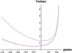
The asymptotic variances of the two estimators are shown in
Figure 1: the curve from BM is always below the other
one, meaning lower values for the asymptotic variance for all values of
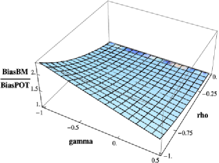
. The asymptotic biases are compared in Figure 2, through the ratio
“bias BM/bias POT”. Recall that the
bias depends on both first- and second-order parameters and
. Contrary to what is observed for the variance, the bias of BM
is always larger but for they are the same regardless the
value of , equal to 1 [or if one takes into account
the asymptotic contribution of to the biases].
Figure 1: Asymptotic variances of PWM estimators with dashed
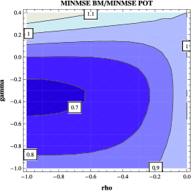
line for POT.Figure 2: Ratio of asymptotic bias of PWM estimators.Figure 3: Contour plot for the ratio of asymptotic minimal mean square
error of PWM estimators.
•
Next, we compare asymptotic mean square errors for
the “optimal choice” of (i.e., that value that makes the limiting
mean square error of minimal), which is different
in the two cases:
An asymptotic expression of the “asymptotic minimal mean square error”
(MINMSE in the sequel) is obtained in the following way.
Suppose . First we find for each estimator the optimal in
the sense of minimizing the approximate asymptotic mean square error.
Denote by and (; “1” refers to PWM-BM and “2” refers to PWM-POT) the
asymptotic variance and squared bias of the estimators. Under Condition 2.1, we can write with decreasing and regularly varying.
The limiting mean square error is, approximately,
(6)
or, writing for , .
Setting the derivative equal to zero and using properties of regularly
varying functions one finds for the optimal choice of ,
and, in terms of ,
Note that the optimal is different but of the same order
for both methods. Next, inserting in (6), after
some manipulation we get the following asymptotic expression for MINMSE,
It follows that MINMSE(BM)/MINMSE(POT) is, approximately,
which does not depend on n, just on and .
The contour plot of “MINMSE(BM)/MINMSE(POT)” is represented in Figure 3. It can be seen that the BM has lower MINMSE for
a large range of combinations. Note that this range
includes negative and positive close to zero which
seem to be common values in many practical situations, for example, in
hydrologic and climatologic extremes. Only for
approximately, MINMSE for POT can be lower depending on .
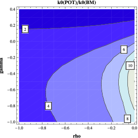
Figure 4: Contour plot for the ratio of the optimal values of .
Finally, comparing the optimal sample sizes (cf. Figure 4 with contour plot of the ratio of the optimal
values of ), one sees that POT requires systematically larger
optimal sample size even when the approximate MINMSE is smaller for POT
than BM.
Quantile estimators
We repeat the previous analysis for the quantile estimators:
•
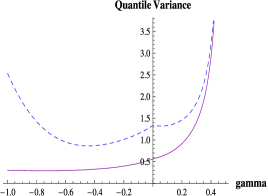
The asymptotic variances of the two estimators are
compared in Figure 5: again the curve from BM is
always below the other one meaning lower values for the asymptotic
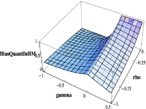
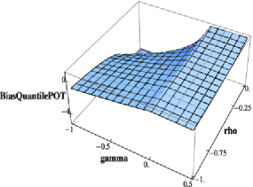
variance for all values of . In Figures 6 and
7, the asymptotic bias is represented for each case
separately. Note that for negative, the bias for BM approaches
zero when whereas in the POT case it escapes to
.
Figure 5: Asymptotic variances of quantile PWM estimators with dashed
line for POT.Figure 6: Asymptotic bias of quantile PWM estimator under BM method.Figure 7: Asymptotic bias of quantile PWM estimator under POT method.
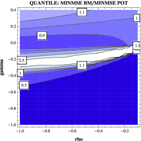
•
The contour plot for the ratio
“MINMSE(BM)/MINMSE(POT)” is represented in Figure 8. Again the BM method has lower MINMSE for a large
range of combinations. The “irregularity” around is due to a change of sign in the bias in the POT case.
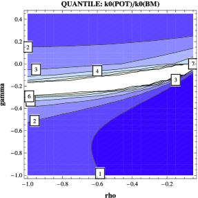
Finally, Figure 9 gives the contour plot for
the ratio of the optimal values of , which is smaller than one when
is small and is closer to zero.
Figure 8: Contour plot for the ratio of asymptotic minimal mean square
error of quantile PWM estimators.Figure 9: Contour plot for the ratio of the optimal values of in
quantile case.
In conclusion, for both the extreme value index and quantile PWM
estimators, the ones from the BM method have always lower asymptotic
variances. Moreover, at an optimal level the BM gives lower MINMSE,
thus being more efficient, under many practical situations. This is in
agreement with some of Sofia Caires’ (2009) conclusions, for example,
that for equal sample sizes or with more than 200 years of data the
uncertainty or the error of the estimates are lower for BM than for POT.
4 Proofs
Throughout this section, represents a unit Fréchet random
variable, that is, one with distribution function ,
, and are the order statistics
from the associated i.i.d. sample of size , .
Similarly,
represents the order statistics of the block maxima
from (1) and, for
, .
Recall the function from Section 2. The following
representation will be useful:
(7)
We start by formulating a number of auxiliary results.
Lemma 4.1
1. As ,
[2.]
2.
[Csörgő and Horváth (1993), page 381]
Let . With
, an appropriate sequence of Brownian bridges,
as ( represents the smallest integer
larger or equal to ).
3.
Similarly, with for an appropriate
sequence of Brownian bridges and ,
as .
The following is an easily obtained variant of Theorem B.3.10 of de Haan and Ferreira (2006).
Lemma 4.2
Under Condition 2.1, there are functions
and , as ,
such that for all there exists
such that for ,
and the statement follows, for example, by Cramér’s delta method.
For the asymptotic distribution of , we write
and the statement follows, for example, by Cramér’s delta method.
{pf*}
Proof of Theorem 2.4
The proof follows the line of the comparable result for the POT method
[see, e.g., de Haan and Ferreira (2006), Chapter 4.3]. Let
. Then
Similarly, as on pages 135–137 of de Haan and Ferreira (2006), this
converges in distribution to
\upqed
Appendix: Asymptotic variances and biases of the PWM estimators
The following provides a basis for an algorithm to calculate the
asymptotic variances/covariances and biases of the PWM estimators.
We would like to thank three unknown referees for their genuine
interest and their insightful comments.
References
Bücher and Segers (2014){barticle}[mr]
\bauthor\bsnmBücher, \bfnmAxel\binitsA. and \bauthor\bsnmSegers, \bfnmJohan\binitsJ.
(\byear2014).
\btitleExtreme value copula estimation based on block maxima of a multivariate stationary time series.
\bjournalExtremes
\bvolume17
\bpages495–528.
\biddoi=10.1007/s10687-014-0195-8, issn=1386-1999, mr=3252823
\bptokimsref\endbibitem
Cai, de Haan and Zhou (2013){barticle}[mr]
\bauthor\bsnmCai, \bfnmJuan-Juan\binitsJ.-J.,
\bauthor\bparticlede \bsnmHaan, \bfnmLaurens\binitsL. and \bauthor\bsnmZhou, \bfnmChen\binitsC.
(\byear2013).
\btitleBias correction in extreme value statistics with index around zero.
\bjournalExtremes
\bvolume16
\bpages173–201.
\biddoi=10.1007/s10687-012-0158-x, issn=1386-1999, mr=3057195
\bptokimsref\endbibitem
Caires (2009){bmisc}[auto:parserefs-M02]
\bauthor\bsnmCaires, \bfnmS.\binitsS.
(\byear2009).
\bhowpublishedA comparative simulation study of the annual maxima
and the peaks-over-threshold methods. SBW-Belastingen: Subproject “Statistics”.
Deltares Report 1200264-002.
\bptokimsref\endbibitem
Csörgő and Horváth (1993){bbook}[mr]
\bauthor\bsnmCsörgő, \bfnmMiklós\binitsM. and \bauthor\bsnmHorváth, \bfnmLajos\binitsL.
(\byear1993).
\btitleWeighted Approximations in Probability and Statistics.
\bpublisherWiley,
\blocationChichester.
\bidmr=1215046
\bptokimsref\endbibitem
Cunnane (1973){barticle}[auto:parserefs-M02]
\bauthor\bsnmCunnane, \bfnmC.\binitsC.
(\byear1973).
\btitleA particular comparison of annual maxima and partial
duration series methods of flood frequency prediction.
\bjournalJ. Hydrol.
\bvolume18
\bpages257–271.
\bptokimsref\endbibitem
de Haan and Ferreira (2006){bbook}[mr]
\bauthor\bparticlede \bsnmHaan, \bfnmLaurens\binitsL. and \bauthor\bsnmFerreira, \bfnmAna\binitsA.
(\byear2006).
\btitleExtreme Value Theory: An Introduction.
\bpublisherSpringer,
\blocationNew York.
\biddoi=10.1007/0-387-34471-3, mr=2234156
\bptokimsref\endbibitem
de Valk (1993){bmisc}[auto:parserefs-M02]
\bauthor\bparticlede \bsnmValk, \bfnmC.\binitsC.
(\byear1993).
\bhowpublishedEstimation of marginals from measurements and hindcast data.
WL—Delft Hydraulics Report H1700.
\bptokimsref\endbibitem
Diebolt et al. (2008){barticle}[mr]
\bauthor\bsnmDiebolt, \bfnmJean\binitsJ.,
\bauthor\bsnmGuillou, \bfnmArmelle\binitsA.,
\bauthor\bsnmNaveau, \bfnmPhilippe\binitsP. and \bauthor\bsnmRibereau, \bfnmPierre\binitsP.
(\byear2008).
\btitleImproving probability-weighted moment methods for the generalized extreme value distribution.
\bjournalREVSTAT
\bvolume6
\bpages35–50.
\bidissn=1645-6726, mr=2386298
\bptokimsref\endbibitem
Dombry (2013){bmisc}[auto:parserefs-M02]
\bauthor\bsnmDombry, \bfnmC.\binitsC.
(\byear2013).
\bhowpublishedMaximum likelihood estimators for the extreme value
index based on the block maxima method.
Available at \arxivurlarXiv:1301.5611.
\bptokimsref\endbibitem
Drees, de Haan and Li (2003){barticle}[mr]
\bauthor\bsnmDrees, \bfnmHolger\binitsH.,
\bauthor\bparticlede \bsnmHaan, \bfnmLaurens\binitsL. and \bauthor\bsnmLi, \bfnmDeyuan\binitsD.
(\byear2003).
\btitleOn large deviation for extremes.
\bjournalStatist. Probab. Lett.
\bvolume64
\bpages51–62.
\biddoi=10.1016/S0167-7152(03)00130-5, issn=0167-7152, mr=1995809
\bptokimsref\endbibitem
Gumbel (1958){bbook}[mr]
\bauthor\bsnmGumbel, \bfnmE. J.\binitsE. J.
(\byear1958).
\btitleStatistics of Extremes.
\bpublisherColumbia Univ. Press,
\blocationNew York.
\bidmr=0096342
\bptokimsref\endbibitem
Hosking (1990){barticle}[mr]
\bauthor\bsnmHosking, \bfnmJ. R. M.\binitsJ. R. M.
(\byear1990).
\btitle-moments: Analysis and estimation of distributions using linear combinations of order statistics.
\bjournalJ. R. Stat. Soc. Ser. B Stat. Methodol.
\bvolume52
\bpages105–124.
\bidissn=0035-9246, mr=1049304
\bptokimsref\endbibitem
Hosking and Wallis (1987){barticle}[mr]
\bauthor\bsnmHosking, \bfnmJ. R. M.\binitsJ. R. M. and \bauthor\bsnmWallis, \bfnmJ. R.\binitsJ. R.
(\byear1987).
\btitleParameter and quantile estimation for the generalized Pareto distribution.
\bjournalTechnometrics
\bvolume29
\bpages339–349.
\biddoi=10.2307/1269343, issn=0040-1706, mr=0906643
\bptokimsref\endbibitem
Hosking, Wallis and Wood (1985){barticle}[mr]
\bauthor\bsnmHosking, \bfnmJ. R. M.\binitsJ. R. M.,
\bauthor\bsnmWallis, \bfnmJ. R.\binitsJ. R. and \bauthor\bsnmWood, \bfnmE. F.\binitsE. F.
(\byear1985).
\btitleEstimation of the generalized extreme-value distribution by the method of probability-weighted moments.
\bjournalTechnometrics
\bvolume27
\bpages251–261.
\biddoi=10.2307/1269706, issn=0040-1706, mr=0797563
\bptokimsref\endbibitem
Katz, Parlange and Naveau (2002){barticle}[auto:parserefs-M02]
\bauthor\bsnmKatz, \bfnmR. W.\binitsR. W.
\bauthor\bsnmParlange, \bfnmM. B.\binitsM. B.
and \bauthor\bsnmNaveau, \bfnmP.\binitsP.
(\byear2002).
\btitleStatistics of extremes in hydrology.
\bjournalAdvances in Water Resources
\bvolume25
\bpages1287–1304.
\bptokimsref\endbibitem
Kharin et al. (2007){barticle}[auto:parserefs-M02]
\bauthor\bsnmKharin, \bfnmV. V.\binitsV. V.,
\bauthor\bsnmZwiers, \bfnmF. W.\binitsF. W.,
\bauthor\bsnmZhang, \bfnmX.\binitsX. and \bauthor\bsnmHegerl, \bfnmG. C.\binitsG. C.
(\byear2007).
\btitleChanges in temperature and precipitation extremes in the IPCC
ensemble of global coupled model simulations.
\bjournalJournal of Climate
\bvolume20
\bpages1419–1444.
\bptokimsref\endbibitem
Landwehr, Matalas and Wallis (1979){barticle}[auto:parserefs-M02]
\bauthor\bsnmLandwehr, \bfnmJ.\binitsJ.,
\bauthor\bsnmMatalas, \bfnmN.\binitsN. and \bauthor\bsnmWallis, \bfnmJ.\binitsJ.
(\byear1979).
\btitleProbability weighted moments compared with some traditional
techniques in estimating Gumbel parameters and quantiles.
\bjournalWater Resources Research
\bvolume15
\bpages1055–1064.
\bptokimsref\endbibitem
Madsen, Pearson and Rosbjerg (1997){barticle}[auto:parserefs-M02]
\bauthor\bsnmMadsen, \bfnmH.\binitsH.,
\bauthor\bsnmPearson, \bfnmC. P.\binitsC. P. and \bauthor\bsnmRosbjerg, \bfnmD.\binitsD.
(\byear1997).
\btitleComparison of annual maximum series and partial duration
series methods for modeling extreme hydrologic events 2. Regional modeling.
\bjournalWater Resources Research
\bvolume33
\bpages759–769.
\bptokimsref\endbibitem
Madsen, Rasmussen and Rosbjerg (1997){barticle}[auto:parserefs-M02]
\bauthor\bsnmMadsen, \bfnmH.\binitsH.,
\bauthor\bsnmRasmussen, \bfnmP. F.\binitsP. F. and \bauthor\bsnmRosbjerg, \bfnmD.\binitsD.
(\byear1997).
\btitleComparison of annual maximum series and partial duration
series methods for modeling extreme hydrologic events 1. At-site modeling.
\bjournalWater Resources Research
\bvolume33
\bpages747–757.
\bptokimsref\endbibitem
Martins and Stedinger (2001){barticle}[auto:parserefs-M02]
\bauthor\bsnmMartins, \bfnmE. S.\binitsE. S. and \bauthor\bsnmStedinger, \bfnmJ. R.\binitsJ. R.
(\byear2001).
\btitleHistorical information in a generalized maximum likelihood
framework with partial duration and annual maximum series.
\bjournalWater Resources Research
\bvolume37
\bpages2559–2567.
\bptokimsref\endbibitem
Naveau et al. (2009){barticle}[mr]
\bauthor\bsnmNaveau, \bfnmPhilippe\binitsP.,
\bauthor\bsnmGuillou, \bfnmArmelle\binitsA.,
\bauthor\bsnmCooley, \bfnmDaniel\binitsD. and \bauthor\bsnmDiebolt, \bfnmJean\binitsJ.
(\byear2009).
\btitleModelling pairwise dependence of maxima in space.
\bjournalBiometrika
\bvolume96
\bpages1–17.
\biddoi=10.1093/biomet/asp001, issn=0006-3444, mr=2482131
\bptokimsref\endbibitem
Pickands (1975){barticle}[mr]
\bauthor\bsnmPickands, \bfnmJames\binitsJ. \bsuffixIII
(\byear1975).
\btitleStatistical inference using extreme order statistics.
\bjournalAnn. Statist.
\bvolume3
\bpages119–131.
\bidissn=0090-5364, mr=0423667
\bptokimsref\endbibitem
Prescott and Walden (1980){barticle}[mr]
\bauthor\bsnmPrescott, \bfnmP.\binitsP. and \bauthor\bsnmWalden, \bfnmA. T.\binitsA. T.
(\byear1980).
\btitleMaximum likelihood estimation of the parameters of the generalized extreme-value distribution.
\bjournalBiometrika
\bvolume67
\bpages723–724.
\biddoi=10.1093/biomet/67.3.723, issn=0006-3444, mr=0601119
\bptokimsref\endbibitem
van den Brink, Können and Opsteegh (2005){barticle}[pbm]
\bauthor\bsnmvan den Brink, \bfnmH. W.\binitsH. W.,
\bauthor\bsnmKönnen, \bfnmG. P.\binitsG. P. and \bauthor\bsnmOpsteegh, \bfnmJ. D.\binitsJ. D.
(\byear2005).
\btitleUncertainties in extreme surge level estimates from observational records.
\bjournalPhilos. Trans. R. Soc. Lond. Ser. A Math. Phys. Eng. Sci.
\bvolume363
\bpages1377–1386.
\biddoi=10.1098/rsta.2005.1573, issn=1364-503X, pii=LL2HPE9025M4UAPF, pmid=16191655
\bptokimsref\endbibitem
Wang (1991){barticle}[auto:parserefs-M02]
\bauthor\bsnmWang, \bfnmQ. J.\binitsQ. J.
(\byear1991).
\btitleThe POT model described by the generalized Pareto distribution
with Poisson arrival rate.
\bjournalJournal of Hidrology
\bvolume129
\bpages263–280.
\bptokimsref\endbibitem