Symmetry breaking for representations of rank one orthogonal groups

Abstract

We give a complete classification of intertwining operators (symmetry breaking operators) between spherical principal series representations of $G=O(n+1,1)$ and $G^{\prime}=O(n,1)$. We construct three meromorphic families of the symmetry breaking operators, and find their distribution kernels and their residues at all poles explicitly. Symmetry breaking operators at exceptional discrete parameters are thoroughly studied.

We obtain closed formulae for the functional equations which the composition of the the symmetry breaking operators with the Knapp–Stein intertwining operators of $G$ and $G^{\prime}$ satisfy, and use them to determine the symmetry breaking operators between irreducible composition factors of the spherical principal series representations of $G$ and $G^{\prime}$. Some applications are included.

Keywords and phrases: branching law, reductive Lie group, symmetry breaking, Lorentz group, conformal geometry, Verma module, complementary series.

2010 MSC: Primary 22E46; Secondary 33C45, 53C35.

1 Introduction

A representation $\pi$ of a group $G$ defines a representation of a subgroup $G^{\prime}$ by restriction. In general irreducibility is not preserved by the restriction. If $G$ is compact then the restriction $\pi|_{G^{\prime}}$ is isomorphic to a direct sum of irreducible representations $\pi^{\prime}$ of $G^{\prime}$ with multiplicities $m(\pi,\pi^{\prime})$. These multiplicities are studied by using combinatorial techniques. If $G^{\prime}$ is not compact and the representation $\pi$ is infinite-dimensional, then generically the restriction $\pi|_{G^{\prime}}$ is not a direct sum of irreducible representations [16] and we have to consider another notion of multiplicity.

For a continuous representation $\pi$ of $G$ on a complete, locally convex topological vector space $H_{\pi}$, the space $H_{\pi}^{\infty}$ of $C^{\infty}$-vectors of $H_{\pi}$ is naturally endowed with a Fréchet topology, and $(\pi,H_{\pi})$ gives rise to a continuous representation $\pi^{\infty}$ of $G$ on $H_{\pi}^{\infty}$. If ${\mathcal{H}}_{\pi}$ is a Banach space, then the Fréchet representation $(\pi^{\infty},{\mathcal{H}}_{\pi}^{\infty})$ depends only on the underlying $({\mathfrak{g}},K)$-module $({\mathcal{H}}_{\pi})_{K}$. Given another continuous representation $\pi^{\prime}$ of the subgroup $G^{\prime}$, we consider the space of continuous $G^{\prime}$-intertwining operators (symmetry breaking operators)

$$\operatorname{Hom}_{G^{\prime}}({\pi}^{\infty}|_{G^{\prime}},({\pi^{\prime}})^{\infty}).$$

The dimension $m(\pi,\pi^{\prime})$ of this space yields important information of the restriction of $\pi$ to $G^{\prime}$ and is called the multiplicity of $\pi^{\prime}$ occurring in the restriction $\pi|_{G^{\prime}}$. Notice that the multiplicity $m(\pi,\pi^{\prime})$ makes sense for non-unitary representations $\pi$ and $\pi^{\prime}$, too. In general, $m(\pi,\pi^{\prime})$ may be infinite. For detailed analysis on symmetry breaking operators, we are interested in the case where $m(\pi,\pi^{\prime})$ is finite. The criterion in [25] asserts that the multiplicity $m(\pi,\pi^{\prime})$ is finite for all irreducible representations $\pi$ of $G$ and all irreducible representations $\pi^{\prime}$ of $G^{\prime}$ if and only if the minimal parabolic subgroup $P^{\prime}$ of $G^{\prime}$ has an open orbit on the real flag variety $G/P$, and that the multiplicity is uniformly bounded with respect to $\pi$ and $\pi^{\prime}$ if and only if a Borel subgroup of $G_{\mathbb{C}}^{\prime}$ has an open orbit on the complex flag variety of $G_{\mathbb{C}}$.

The classification of reductive symmetric pairs $({\mathfrak{g}},{\mathfrak{g}}^{\prime})$ satisfying the former condition was recently accomplished in [20]. On the other hand, the latter condition depends only on the complexified pairs $({\mathfrak{g}}_{\mathbb{C}},{\mathfrak{g}}_{\mathbb{C}}^{\prime})$, for which the classification is much simpler and was already known in 1970s by Krämer [28]. In particular, the multiplicity $m(\pi,\pi^{\prime})$ is uniformly bounded if the Lie algebras $({\mathfrak{g}},{\mathfrak{g}}^{\prime})$ of $(G,G^{\prime})$ are real forms of $({\mathfrak{sl}}(N+1,{\mathbb{C}}),{\mathfrak{gl}}(N,{\mathbb{C}}))$ or $({\mathfrak{o}}(N+1,{\mathbb{C}}),{\mathfrak{o}}(N,{\mathbb{C}}))$.

In this article we confine ourselves to the case

$$(G,G^{\prime})=(O(n+1,1),O(n,1)),$$ (1.1)

and study thoroughly symmetry breaking operators between spherical principal series representations for the groups $G$ and $G^{\prime}$. In particular, we determine the multiplicities for their composition factors. Furthermore, we give a classification of symmetry breaking operators $I(\lambda)^{\infty}\to J(\nu)^{\infty}$ for any spherical principal series representations $I(\lambda)$ and $J(\nu)$, and find explicit formulae of distribution kernels of its basis for every $(\lambda,\nu)\in{\mathbb{C}}^{2}$.

The techniques of this article are actually directed at the more general problems of determining symmetry breaking operators between (degenerate) principal series representations induced from parabolic subgroups $P$ of $G$ and $P^{\prime}$ of $G^{\prime}$ under the geometric assumption that the double coset $P^{\prime}\backslash G/P$ is a finite set. In the setting (1.1), there are three (nonempty) closed $P^{\prime}$-invariant subsets in $G/P$. Correspondingly, we construct a family of (generically) regular symmetry breaking operators $\widetilde{\mathbb{A}}_{\lambda,\nu}$ and two families of singular symmetry ones $\widetilde{\mathbb{B}}_{\lambda,\nu}$ and $\widetilde{\mathbb{C}}_{\lambda,\nu}$.

The classification of symmetry breaking operators $T$ is carried out through an analysis of their distribution kernels $K_{T}$. We consider the system of partial differential equations that $K_{T}$ satisfies, and determine when an (obvious) local solution along a $P^{\prime}$-orbit extends to a global solution on the whole real flag variety $G/P$. The important properties of these symmetry breaking operators are the existence of the meromorphic continuation, and the functional equations that they satisfy with the Knapp–Stein intertwining operators of $G$ and $G^{\prime}$. The residue calculus of $\widetilde{\mathbb{A}}_{{\lambda},{\nu}}$ provides a third method to obtain Juhl’s conformally covariant operators $\widetilde{\mathbb{C}}_{\lambda,\nu}$ for the embedding $S^{n-1}\hookrightarrow S^{n}$ (see [13], [17] for the two earlier proofs, and [18] for a heuristic argument for the method of this article).

To state our results more precisely, we realize $G=O(n+1,1)$ as the automorphism group of a quadratic form

$$x^{2}_{0}+x^{2}_{1}+\cdots+x^{2}_{n}-x^{2}_{n+1}$$

and the subgroup $G^{\prime}=O(n,1)$ as the stabilizer of the basis vector $e_{n}={}^{t\!}(0,\cdots,0,1,0)$.

A spherical principal series representation $I(\lambda)$ of $G$ is an (unnormalized) induced representation from a character $\chi_{\lambda}$ of a minimal parabolic subgroup $P$ for $\lambda\in{\mathbb{C}}$. In what follows, we take the representation space of $I(\lambda)$ to be the space of $C^{\infty}$-sections of the $G$-equivariant line bundle $G\times_{P}(\chi_{\lambda},{\mathbb{C}})\to G/P$, so that $I(\lambda)^{\infty}\simeq I(\lambda)$ is the Fréchet globalization having moderate growth in the sense of Casselman–Wallach [39]. See Section 3.4. The parametrization is chosen so that $I(\lambda)$ is reducible if and only if $-\lambda\in{\mathbb{N}}$ or $\lambda-n\in{\mathbb{N}}$, and that $I(-i)$ ($i\in{\mathbb{N}}$) contains a finite-dimensional representation $F(i)$ as the unique subrepresentation, which is isomorphic to the representation on the space ${\mathcal{H}}^{i}({\mathbb{R}}^{n+1,1})$ of spherical harmonics of degree $i$ as a representation of the identity component $G_{0}$ of $G$, see (2.14). The irreducible Fréchet representation $I(-i)/F(i)$ of $G$ is denoted by $T(i)$. The underlying $({\mathfrak{g}},K)$-module $T(i)_{K}$ is isomorphic to a Zuckerman $A_{\mathfrak{q}}(\lambda)$-modules where ${\mathfrak{q}}$ is a certain maximal $\theta$-stable parabolic subalgebra of ${\mathfrak{g}}_{\mathbb{C}}$ (see Section 16.3). In this parametrization, $I(\lambda)$ is unitarizable if $\lambda\in\frac{n}{2}+\sqrt{-1}{\mathbb{R}}$ (unitary principal series representation) or $0<\lambda<n$ (complementary series representations, see Chapter 15).

Similarly, spherical principal series representations of the subgroup $G^{\prime}$ are denoted by $J(\nu)$ and are parametrized so that the finite-dimensional representations $F(j)$ is a subrepresentation of $J(-j)$. The irreducible Fréchet representation $J(-j)/F(j)$ of $G^{\prime}$ is denoted by $T(j)$.

Consider pairs of nonpositive integers and define

$$L_{\operatorname{even}}:= \left\{(-i,-j):j\leq i\mbox{ and }i\equiv j\mod 2\right\},$$

$$L_{\operatorname{odd}}:= \left\{(-i,-j):j\leq i\mbox{ and }i\equiv j+1\mod 2\right\}.$$

The discrete set $L_{\operatorname{even}}$ in ${\mathbb{C}}^{2}$ plays a special role throughout the article. We prove:

Theorem 1.1 (multiplicities for spherical principal series, Theorem 11.4).

We have

$$m(I(\lambda),J(\nu))=\begin{cases}1\qquad&\text{if $(\lambda,\nu)\in{\mathbb{C}}^{2}-L_{\operatorname{even}}$, }\\ 2\qquad&\text{if $(\lambda,\nu)\in L_{\operatorname{even}}$.}\end{cases}$$

This theorem is new even for $G=O(3,1)\approx PGL(2,\mathbb{C})$ and $G^{\prime}=O(2,1)\approx PGL(2,\mathbb{R})$.

From the viewpoint of differential geometry, $G$ is the conformal group of the standard sphere $S^{n}$, and conformally equivariant line bundles ${\mathcal{L}}_{\lambda}$ over $S^{n}$ are parametrized by $\lambda\in{\mathbb{C}}$ (we normalize ${\mathcal{L}}_{\lambda}$ such that ${\mathcal{L}}_{0}$ is the trivial line bundle and ${\mathcal{L}}_{n}$ is the bundle of volume densities). The subgroup $G^{\prime}$ is the conformal group of the ‘great circle’ $S^{n-1}$ in $S^{n}$, and conformally equivariant line bundles ${\mathcal{L}}_{\nu}$ over $S^{n-1}$ are parametrized by $\nu\in{\mathbb{C}}$. Then Theorem 1.1 determines the dimension of conformally covariant linear maps (i.e., $G^{\prime}$-equivariant operators) from $C^{\infty}(S^{n},{\mathcal{L}}_{\lambda})$ to $C^{\infty}(S^{n-1},{\mathcal{L}}_{\nu})$.

From the representation theoretic viewpoint, it was proved recently in Sun and Zhu [35] that $m(\pi,\pi^{\prime})\leq 1$ for all irreducible admissible representations $\pi$ of $G$ and $\pi^{\prime}$ of $G^{\prime}$. However, it is much more involved to tell whether $m(\pi,\pi^{\prime})=0$ or $1$ for given irreducible representations $\pi$ and $\pi^{\prime}$.

The following theorem determines $m(\pi,\pi^{\prime})$ for irreducible subquotients at reducible points.

Theorem 1.2 (multiplicities for composition factors, Theorem 2.5).

Let $i,j\in{\mathbb{N}}$.

1. Suppose that $i\geq j$.

   (1-a)  Assume $i\equiv j\mod 2$, namely, $(-i,-j)\in L_{\operatorname{even}}$. Then

   $$m(T(i),T(j))=1,\qquad m(T(i),F(j))=0,\qquad m(F(i),F(j))=1.$$

   (1-b)  Assume $i\equiv j+1\mod 2$, namely, $(-i,-j)\in L_{\operatorname{odd}}$. Then

   $$m(T(i),T(j))=0,\qquad m(T(i),F(j))=1,\qquad m(F(i),F(j))=0.$$

2. Suppose that $i<j$. Then

   $$m(T(i),T(j))=0,\quad m(T(i),F(j))=1,\quad m(F(i),F(j))=0.$$

Similar results were obtained by Loke [29] for the $(\mathfrak{g},K)$-modules of representations of $G=GL(2,{\mathbb{C}})$ and $G^{\prime}=GL(2,{\mathbb{R}})$.

We also determine the multiplicity of (possibly, reducible) spherical principal series representations $I(\lambda)$ of $G$ and irreducible finite-dimensional representations $F(j)$, respectively infinite-dimensional ones $T(j)$ of the subgroup $G^{\prime}$ in Theorem 2.6:

Theorem 1.3.

Suppose $j\in{\mathbb{N}}$.

1. $m(I(\lambda),F(j))=1\quad\quad\text{for all }\,\,\lambda\in{\mathbb{C}}.$

2. $m(I(\lambda),T(j))=\begin{cases}1\quad&\text{if }\,\,\lambda+j\in-2{\mathbb{N}},\\ 0\quad&\text{if }\,\,\lambda+j\not\in-2{\mathbb{N}}.\end{cases}$

In the special case $\nu=0$, our results on symmetry breaking operators are closely related to the analysis on the indefinite hyperbolic space

$$X(n+1,1):=\{\xi\in\mathbb{R}^{n+2}:\xi_{0}^{2}+\dots+\xi_{n}^{2}-\xi_{n+1}^{2}=1\}\simeq G/G^{\prime}.$$

As a hypersurface of the Minkowski space

$$\mathbb{R}^{n+1,1}\equiv(\mathbb{R}^{n+2},d\xi_{0}^{2}+\dots+d\xi_{n}^{2}-d\xi_{n+1}^{2}),$$

$X(n+1,1)$ carries a Lorentz metric for which the sectional curvature is constant $-1$, and thus is a model space of anti-de Sitter manifolds. The Laplacian $\Delta$ of the Lorentz manifold $X(n+1,1)$ is a hyperbolic operator, and for $\lambda\in\mathbb{C}$, we consider its eigenspace:

$$\mathcal{S}ol(G/G^{\prime};\lambda):=\{f\in\mathcal{C}^{\infty}(G/G^{\prime}):\Delta f=-\lambda(\lambda-n)f\}.$$

The underlying $(\mathfrak{g},K)$-module $\mathcal{S}ol(G/G^{\prime};\lambda)_{K}$ is isomorphic to the underlying $(\mathfrak{g},K)$-module of a principal series representation [32]. For $\lambda=-i\in-\mathbb{N}$ there are two inequivalent reducible principal series representations $I(-i)_{K}$ and $I(n+i)_{K}$, and our results on the symmetry breaking operators $\widetilde{\mathbb{A}}_{\lambda,0}$ for $(\lambda,0)\in L_{\operatorname{even}}$ give another proof of the following $(\mathfrak{g},K)$-isomorphism:

$$\mathcal{S}ol(G/G^{\prime};\lambda)_{K}\simeq\begin{cases}I(-i)_{K}\qquad&\text{if }\lambda=-i\in-2{\mathbb{N}},\\ I(n+i)_{K}\qquad&\text{if }\lambda=-i\in-2{\mathbb{N}}-1.\end{cases}$$

More generally, we apply our results on symmetry breaking operators for $\nu\in-{\mathbb{N}}$ to the analysis on vector bundles. We note that harmonic analysis on (general) semisimple symmetric spaces has been studied actively by many people during the last fifty years, however, not much has been known for vector bundle sections. We construct in Theorem 14.9 some irreducible subrepresentations in the space of sections of the $G$-equivariant vector bundles $G\times_{G^{\prime}}F(j)\to G/G^{\prime}$ by using symmetry breaking operators $\widetilde{\mathbb{A}}_{\lambda,\nu}$.

We also obtain branching laws for unitary complementary series representations of $I(\lambda)$ $(0<\lambda<n)$, which by abuse of notation we also denote by $I(\lambda)$. For $\lambda\in{\mathbb{R}}$, we set

$$D(\lambda):=\{\nu\in\lambda-1+2{\mathbb{Z}}:\frac{n-1}{2}<\nu\leq\lambda-1\}.$$

Then $D(\lambda)$ is a finite set, and $D(\lambda)$ is non-empty if and only if $\lambda>\frac{n+1}{2}$. As an application of differential symmetry breaking operators $\widetilde{\mathbb{C}}_{\lambda,\nu}$, we have

Theorem 1.4 (branching law of complementary series, Theorem 15.1).

Suppose that $\frac{n+1}{2}<\lambda<n$. Then $J(\nu)$ is a complementary series representation of the subgroup $G^{\prime}$ for any $\nu\in D(\lambda)$. Moreover, the restriction of $I(\lambda)$ to $G^{\prime}$ contains the finite sum $\bigoplus_{\nu\in D(\lambda)}J(\nu)$ as discrete summands.

About 20 years ago Gross and Prasad [7] formulated a conjecture about the restriction of an irreducible admissible tempered representation of an inner form $G$ of the group $O(n)$ over a local field to a subgroup $G^{\prime\prime}$ which is an inner form $G^{\prime}=O(n-1)$. The conjecture in [7] relates the existence of nontrivial homomorphisms to the value of an L-function at 1/2 and the value of the epsilon factor. We expect to come back to this in a later paper.

Let us enter the proof of Theorem 1.1 and its refinement (Theorem 1.9 below) in a little more details. We first construct an analytic family of (generically) regular symmetry breaking operators and show

Theorem 1.5 (regular symmetry breaking operators, Theorem 8.1).

There exists a family of symmetry breaking operators $\widetilde{\mathbb{A}}_{\lambda,\nu}\in\operatorname{Hom}_{G^{\prime}}(I(\lambda),J(\nu))$ that depends holomorphically for entire $(\lambda,\nu)\in{\mathbb{C}}^{2}$ with the distribution kernel

$$\widetilde{K}_{{\lambda},{\nu}}^{\mathbb{A}}(x,x_{n}):=\frac{1}{\Gamma(\frac{\lambda+\nu-n+1}{2})\Gamma(\frac{\lambda-\nu}{2})}|x_{n}|^{\lambda+\nu-n}(|x|^{2}+x_{n}^{2})^{-\nu}.$$

Further, $\widetilde{\mathbb{A}}_{\lambda,\nu}$ is nonzero if and only if $(\lambda,\nu)\in{\mathbb{C}}^{2}-L_{\operatorname{even}}$.

We recall that there exist nonzero Knapp–Stein intertwining operators

$\widetilde{\mathbb{T}}_{{\nu}}:J(\nu)\rightarrow J(n-1-\nu)$     and    $\widetilde{\mathbb{T}}_{{\lambda}}:I(\lambda)\rightarrow I(n-\lambda),$

with holomorphic parameters $\nu\in{\mathbb{C}}$ and $\lambda\in\mathbb{C}$, respectively. In our normalization

$$\widetilde{\mathbb{T}}_{{n-1-\nu}}\circ\widetilde{\mathbb{T}}_{{\nu}}= \frac{\pi^{n-1}}{\Gamma(n-1-\nu)\Gamma(\nu)}\operatorname{id}\quad \text{on }J(\nu),$$

and

$$\widetilde{\mathbb{T}}_{{n-\lambda}}\circ\widetilde{\mathbb{T}}_{{\lambda}}= \frac{\pi^{n}}{\Gamma(n-\lambda)\Gamma(\lambda)}\operatorname{id}\quad \text{on }I(\lambda).$$

The following functional identities are crucial in the proof of Theorems 1.5 and 1.11.

Theorem 1.6 (functional identities, Theorem 8.5).

For all $(\lambda,\nu)\in{\mathbb{C}}^{2}$,

$$\widetilde{\mathbb{T}}_{{n-1-\nu}}\circ\widetilde{\mathbb{A}}_{\lambda,n-1-\nu}= \frac{\pi^{\frac{n-1}{2}}}{\Gamma(n-1-\nu)}\widetilde{\mathbb{A}}_{\lambda,\nu},$$ (1.2)

$$\widetilde{\mathbb{A}}_{n-\lambda,\nu}\circ\widetilde{\mathbb{T}}_{{\lambda}}= \frac{\pi^{\frac{n}{2}}}{\Gamma(n-\lambda)}\widetilde{\mathbb{A}}_{\lambda,\nu}.$$ (1.3)

Here $\widetilde{\mathbb{T}}_{{n-1-\nu}}$ and $\widetilde{\mathbb{T}}_{{\lambda}}$ are the Knapp–Stein intertwining operators of $G^{\prime}$ and $G$, respectively. If $\nu-n+1\in{\mathbb{N}}$ or $\lambda-n\in{\mathbb{N}}$, then the left-hand side of (1.2) or (1.3) is zero, respectively.

The functional identities in Theorem 1.6 are extended to other families of singular breaking symmetry operators (see Theorem 12.6, Corollary 12.7, and Corollary 12.8).

We construct other families of symmetry breaking operators as follows: We define

$$//:= \{(\lambda,\nu)\in{\mathbb{C}}^{2}:\lambda-\nu=0,-2,-4,\dots\},$$

$$\backslash\backslash:= \{(\lambda,\nu)\in{\mathbb{C}}^{2}:\lambda+\nu=n-1,n-3,n-5\dots\},$$

$$\mathbb{X}:= \backslash\backslash\cap//.$$

We note

$$L_{\operatorname{even}}\subset\begin{cases}{\mathbb{X}}&\text{if $n$ is odd,}\\ /\!/-\backslash\!\backslash&\text{if $n$ is even.}\end{cases}$$ (1.4)

For $\nu\in-{\mathbb{N}}$, the renormalized operator $\tilde{\tilde{\mathbb{A}}}_{\lambda,\nu}:=\Gamma(\frac{\lambda-\nu}{2}){\widetilde{\mathbb{A}}}_{\lambda,\nu}$ extends to a non-zero $G^{\prime}$-intertwining map, that depends holomorphically on $\lambda\in{\mathbb{C}}$.

For $(\lambda,\nu)\in\backslash\!\backslash$, we define a family of singular $G^{\prime}$-intertwining operators $\widetilde{{\mathbb{B}}}_{\lambda,\nu}:I(\lambda)\to J(\nu)$ that depends holomorphically on $\lambda\in\mathbb{C}$ (or on $\nu\in\mathbb{C}$) by the distribution kernel

$$\widetilde{K}_{{\lambda},{\nu}}^{\mathbb{B}}(x,x_{n}):=\frac{1}{\Gamma(\frac{\lambda-\nu}{2})}(|x|^{2}+x_{n}^{2})^{-\nu}\delta^{(2k)}(x_{n}).$$

For $(\lambda,\nu)\in//$, we set $l:=\frac{1}{2}(\nu-\lambda)$ and define a differential operator

$$\widetilde{\mathbb{C}}_{\lambda,\nu}=\operatorname{rest}\circ\sum_{j=0}^{l}\frac{2^{2l-2j}}{j!(2l-2j)!}\prod_{i=1}^{l-j}\Bigl{(}\frac{\lambda+\nu-n-1}{2}+i\Bigr{)}\Delta_{\mathbb{R}^{n-1}}^{j}\Bigl{(}\frac{\partial}{\partial x_{n}}\Bigr{)}^{2l-2j}.$$

Here $\operatorname{rest}$ denotes the restriction to the hyperplane $x_{n}=0$. It gives a differential symmetry breaking operator $\widetilde{{\mathbb{C}}}_{\lambda,\nu}:I(\lambda)\rightarrow J(\nu)$ of order $2l$, and coincides with the conformally covariant differential operator for the embedding $S^{n-1}\hookrightarrow S^{n}$, which was discovered recently by A. Juhl in [13].

Using the support of the operators, we prove the following refinement of Theorem 1.1. We show:

Proposition 1.7.

Every operator in $\operatorname{Hom}_{G^{\prime}}(I(\lambda),J(\nu))$ is in the ${\mathbb{C}}$-span of the operators $\widetilde{\mathbb{A}}_{\lambda,\nu}$, $\widetilde{\widetilde{\mathbb{A}}}_{\lambda,\nu}$, $\widetilde{{\mathbb{B}}}_{\lambda,\nu}$ and $\widetilde{{\mathbb{C}}}_{\lambda,\nu}$.

Examining the linear independence of symmetry breaking operators constructed above we prove

Theorem 1.8 (residue formulae, Theorem 12.2).

1. For $(\lambda,\nu)\in\backslash\!\backslash-\mathbb{X}$, we define $k:=\frac{1}{2}(n-1-\lambda-\nu)\in\mathbb{N}$. Then

   $$\widetilde{{\mathbb{A}}}_{\lambda,\nu}=\frac{(-1)^{k}}{2^{k}(2k-1)!!}\widetilde{{\mathbb{B}}}_{\lambda,\nu}.$$

2. For $(\nu,\lambda)\in/\!/$, we define $l:=\frac{1}{2}(\nu-\lambda)$. Then

   $$\widetilde{{\mathbb{A}}}_{\lambda,\nu}=\frac{(-1)^{l}l!\pi^{\frac{n-1}{2}}}{\Gamma(\nu)2^{2l}}\widetilde{{\mathbb{C}}}_{\lambda,\nu}.$$

3. Suppose $(\lambda,\nu)\in\mathbb{X}$. We define $k,l\in\mathbb{N}$ as above. Then

   $$\widetilde{{\mathbb{B}}}_{\lambda,\nu}=\frac{(-1)^{l-k}2^{k-2l}\pi^{\frac{n-1}{2}}l!(2k-1)!!}{\Gamma(\nu)}\widetilde{{\mathbb{C}}}_{\lambda,\nu}.$$

Theorem 1.8 implies that singular symmetry breaking operators $\widetilde{\mathbb{B}}_{\lambda,\nu}$ and $\widetilde{\mathbb{C}}_{\lambda,\nu}$ can be obtained as the residues of the meromorphic family of (generically) regular symmetry breaking operators in most cases. An exception happens for the differential symmetry breaking operator $\widetilde{\mathbb{C}}_{\lambda,\nu}$ for $(\lambda,\nu)\in L_{\operatorname{even}}$ (see also Remark 12.4). In fact the dimension of $\operatorname{Hom}_{G^{\prime}}(I(\lambda),J(\nu))$ jumps at $(\lambda,\nu)\in L_{\operatorname{even}}$ as we have seen in Theorem 1.1.

We prove a stronger form of Theorem 1.1 by giving an explicit basis of symmetry breaking operators:

Theorem 1.9 (explicit basis, Theorem 11.3).

For $(\lambda,\nu)\in{\mathbb{C}}^{2}$, we have

$$\operatorname{Hom}_{G^{\prime}}(I(\lambda),J(\nu))=\begin{cases}\mathbb{C}\widetilde{\widetilde{{\mathbb{A}}}}_{\lambda,\nu}\oplus\mathbb{C}\tilde{{\mathbb{C}}}_{\lambda,\nu}&\text{if\/ $(\lambda,\nu)\in L_{\operatorname{even}}$},\\ \mathbb{C}\widetilde{{\mathbb{A}}}_{\lambda,\nu}&\text{if\/ $(\lambda,\nu)\in\mathbb{C}^{2}-L_{\operatorname{even}}$}.\end{cases}$$

Denote by $\mathbf{1}_{\lambda}$ and $\mathbf{1}_{\nu}$ the normalized spherical vectors in $I(\lambda)$ and $J(\nu)$, respectively. The image of spherical vector $\mathbf{1}_{\lambda}$ under the symmetry breaking operators $\widetilde{\mathbb{A}}_{\lambda,\nu}$ and $\widetilde{\mathbb{B}}_{\lambda,\nu}$ is nonzero if and only if $\lambda\not=0,-1,-2,-3\dots$, whereas it is always nonzero under $\widetilde{\mathbb{C}}_{\lambda,\nu}$. More precisely we prove in Propositions 7.4, 9.6, and 10.7 the following:

Theorem 1.10 (transformations of spherical vectors).

1. For $(\lambda,\nu)\in\mathbb{C}^{2}$,

   $$\widetilde{{\mathbb{A}}}_{\lambda,\nu}(\mathbf{1}_{\lambda})=\frac{\pi^{\frac{n-1}{2}}}{\Gamma(\lambda)}\mathbf{1}_{\nu}.$$

2. For $(\lambda,\nu)\in\backslash\!\backslash$, we set $k:=\frac{1}{2}(n-1-\lambda-\nu)$. Then

   $$\widetilde{{\mathbb{B}}}_{\lambda,\nu}(\mathbf{1}_{\lambda})=\frac{(-1)^{k}2^{k}\pi^{\frac{n-1}{2}}(2k-1)!!}{\Gamma(\lambda)}\mathbf{1}_{\nu}.$$

3. For $(\lambda,\nu)\in/\!/$, we set $l:=\frac{1}{2}(\nu-\lambda)\in\mathbb{N}$. Then

   $$\widetilde{{\mathbb{C}}}_{\lambda,\nu}(\mathbf{1}_{\lambda})=\frac{(-1)^{l}2^{2l}(\lambda)_{2l}}{l!}\mathbf{1}_{\nu}.$$

We also determine the image of the underlying $({\mathfrak{g}},K)$-module $I(\lambda)_{K}$ of $I(\lambda)$ by the symmetry breaking operators for all the parameters $(\lambda,\nu)\in{\mathbb{C}}^{2}$. Using the basis in Theorem 1.9, we have:

Theorem 1.11 (image of breaking symmetry operator, see Theorems 13.1 and 13.2).

(1) Suppose that $(\lambda,\nu)\in L_{\operatorname{even}}$ and set $j:=-\nu\in{\mathbb{N}}$. Then

$$\operatorname{Image}\tilde{\tilde{\mathbb{A}}}_{\lambda,\nu}=F(j)$$

and

$$\operatorname{Image}\widetilde{\mathbb{C}}_{{\lambda},{\nu}}=J(\nu)_{K^{\prime}}.$$

(2) Suppose that $(\lambda,\nu)\not\in L_{\operatorname{even}}$. Then

$${\rm{(2\text{-}a)}}\qquad \operatorname{Image}\widetilde{\mathbb{A}}_{{\lambda},{\nu}}=F(-\nu)\quad \text{if }\nu\in-{\mathbb{N}},$$

$${\rm{(2\text{-}b)}} \operatorname{Image}\widetilde{\mathbb{A}}_{{\lambda},{\nu}}=T(\nu+1-n)_{K^{\prime}}\quad \text{if }(\lambda,\nu)\in\backslash\backslash\quad\text{and }\nu+1-n\in{\mathbb{N}},$$

$${\rm{(2\text{-}c)}} \operatorname{Image}\widetilde{\mathbb{A}}_{{\lambda},{\nu}}=J(\nu)_{K^{\prime}}\quad \text{otherwise}.$$

The outline of the article is as follows:

Before we start with the construction of the intertwining operators between spherical principal series representations of $G=O(n+1,1)$ and $G^{\prime}=O(n,1)$ we prove in Chapter 2 our main results about $G^{\prime}$-intertwining operators between irreducible composition factors of spherical principal series representations (Theorem 1.2). In this proof we use the results about symmetry breaking operators for spherical principal series representations of $G$ and $G^{\prime}$ (Theorem 1.9) and their functional equations (Theorem 1.6) proved later in the article.

Chapter 3 gives a general method to study symmetry breaking operators for (smooth) induced representations by means of their distribution kernels. Analyzing their supports we obtain a natural filtration of the space of symmetry breaking operators induced from the closure relation on the double coset $P^{\prime}\backslash G/P$ in Section 3.3, which will be used later to estimate the dimension of $\operatorname{Hom}_{G^{\prime}}(I(\lambda),J(\nu))$.

In Chapter 4 we give preliminary results on spherical principal series representations such as explicit formulae for the realization in the noncompact picture $C^{\infty}(\mathbb{R}^{n})$ using the open Bruhat cell. Then we recall the Knapp–Stein intertwining operator ${\mathbb{T}}_{{\lambda}}$, define a normalized operator $\widetilde{\mathbb{T}}_{{\lambda}}$, and show some of its properties. Notice that our normalization arises from analytic considerations and is not the same as the normalization introduced by Knapp and Stein.

Chapter 5 is a discussion of the double coset decompositions $G^{\prime}\backslash G/P$ and $P^{\prime}\backslash G/P$. We prove in particular that $G=P^{\prime}N_{-}P$.

In Chapter 6 we derive a system of differential equations on $\mathbb{R}^{n}$ and show in Proposition 6.5 that its distribution solutions $\mathcal{S}ol(\mathbb{R}^{n};\lambda,\nu)$ are isomorphic to $\operatorname{Hom}_{G^{\prime}}(I(\lambda),J(\nu))$. An analysis of the solutions shows that generically the multiplicity $m(I(\lambda),J(\nu))$ of principal series representations is 1 (see Theorem 1.1).

In Chapter 7 we use the distribution $K^{\mathbb{A}}_{\lambda,\nu}\in\mathcal{S}ol(\mathbb{R}^{n};\lambda,\nu)$ to define for $(\lambda,\nu)$ in an open region $\Omega_{0}$ a $(\mathfrak{g}^{\prime},K^{\prime})$-homomorphism $\widetilde{\mathbb{A}}_{\lambda,\nu}:I(\lambda)_{K}\to J(\nu)_{K^{\prime}}$. Normalizing the distribution kernel by a Gamma factor we obtain an operator $\widetilde{\mathbb{A}}_{\lambda,\nu}$ and prove that $\widetilde{\mathbb{A}}_{\lambda,\nu}(\varphi)$ is holomorphic in $(\lambda,\nu)\in\mathbb{C}^{2}$ for every $\varphi\in I(\lambda)_{K}$, and that $\widetilde{\mathbb{A}}_{\lambda,\nu}(\varphi)=0$ for all $\varphi\in I(\lambda)_{K}$ if and only if $(\lambda,\nu)\in L_{\operatorname{even}}$.

In Chapter 8 we prove the existence of the meromorphic continuation of ${\mathbb{A}}_{\lambda,\nu}$, initially defined holomorphically on the parameter $(\lambda,\nu)$ in the open region $\Omega_{0}$, to $(\lambda,\nu)$ in the entire $\mathbb{C}^{2}$. Besides, we determine all the poles of the symmetry breaking operator ${\mathbb{A}}_{{\lambda},{\nu}}$ with meromorphic parameter $\lambda$ and $\nu$ and show that the normalized symmetry breaking operators $\widetilde{\mathbb{A}}_{{\lambda},{\nu}}:I(\lambda)\to J(\nu)$ depend holomorphically on ${{\lambda},{\nu}}$. Here we use and prove the functional equations (Theorem 1.6) of the symmetry breaking operators.

An analysis on the exceptional discrete set $L_{\operatorname{even}}$ is particularly important. We introduce for $\nu\in-{\mathbb{N}}$ a different normalization to obtain nonzero operators $\widetilde{\widetilde{\mathbb{A}}}_{{\lambda},{\nu}}$ for $(\lambda,\nu)\in L_{\operatorname{even}}$.

In Chapter 9 we start the discussion of the singular symmetry breaking operators for $(\lambda,\nu)\in\backslash\backslash$, their analytic continuation and find a necessary and sufficient condition which determines if they are not zero.

Chapter 10 is a discussion of the differential symmetry breaking operators, which were first found by Juhl.

Building on these preparations, we complete in Chapter 11 the classification of symmetry breaking operators from the spherical principal series representation $I(\lambda)$ of $G=O(n+1,1)$ to the representations $J(\nu)$ of $G^{\prime}=O(n,1)$ and prove Theorems 1.1 and 1.9. Here again the analysis of $\mathcal{S}ol(\mathbb{R}^{n};\lambda,\nu)$ for the parameter in $\backslash\backslash$ and $//$ plays a crucial role.

In Chapter 12 we show the relationships among the (generically) regular symmetry breaking operators $\widetilde{\mathbb{A}}_{\lambda,\nu}$, the singular symmetry breaking operators $\widetilde{\mathbb{B}}_{\lambda,\nu}$ and the differential symmetry breaking operators $\widetilde{\mathbb{C}}_{\lambda,\nu}$ by proving explicitly the residue formulae (Theorem 1.10). Furthermore we also extend the functional equations to these singular symmetry breaking operators.

Finally, Theorem 1.10 (1), (2), and (3) are proved by explicit computations in Chapters 7, 9, and 10, respectively, and Theorem 1.11 is proved by using Theorem 1.10 in Chapter 13.

The last two chapters are applications of our results. In Chapter 14 we apply our results about symmetry breaking operators $\widetilde{\mathbb{A}}_{\lambda,\nu}$ to the analysis on vector bundles over the semisimple symmetric space $O(n+1,1)/O(n,1)$. In Chapter 15 we construct explicitly complementary series representations of the group $G^{\prime}=O(n,1)$ as discrete summands in the restriction of the unitary complementary series representations of $O(n+1,1)$ by using the adjoint of the differential symmetry breaking operators $\widetilde{\mathbb{C}}_{\lambda,\nu}$

Notation. ${\mathbb{N}}=\{0,1,2,\cdots\}$, ${\mathbb{N}}_{+}=\{1,2,3,\cdots\}$, ${\mathbb{R}}^{\times}={\mathbb{R}}-\{0\}$. For two subsets $A$ and $B$ of a set, we write

$$A-B:=\{a\in A:a\notin B\}$$

rather than the usual notation $A\backslash B$.

2 Symmetry breaking for the spherical principal series representations

Before we start with the construction of the $G^{\prime}$-intertwining operators between spherical principal series representations of $G=O(n+1,1)$ and $G^{\prime}=O(n,1)$ we want to prove the main results (Theorems 1.2 and 1.3, see Theorems 2.5 and 2.6 below) about $G^{\prime}$-intertwining operators between irreducible composition factors of spherical principal series representations. This is intended for the convenience of the readers who are more interested in representation theoretic results rather than geometric analysis arising from branching problems in representation theory. In the proof we use the results about symmetry breaking operators for spherical principal series representations of $G$ and $G^{\prime}$ that will be proved later in the article.

2.1 Notation and review of previous results

Consider the quadratic form

$$x_{0}^{2}+x_{1}^{2}+\dots+x_{n}^{2}-x_{n+1}^{2}$$ (2.1)

of signature $(n+1,1)$. We define $G$ to be the indefinite orthogonal group $O(n+1,1)$ that preserves the quadratic form (2.1). Let $G^{\prime}$ be the stabilizer of the vector $e_{n}={}^{t}\!(0,0,\cdots,0,1,0)$. Then $G^{\prime}\simeq O(n,1)$. We set

$$K:= O(n+1)\times O(1),$$ (2.2)

$$K^{\prime}:= K\cap G^{\prime}=\{\begin{pmatrix}A&&\\ &1&\\ &&\varepsilon\end{pmatrix}:A\in O(n),\varepsilon=\pm 1\}\simeq O(n)\times O(1).$$ (2.3)

Then $K$ and $K^{\prime}$ are maximal compact subgroups of $G$ and $G^{\prime}$, respectively.

Let ${\mathfrak{g}}={\mathfrak{o}}(n+1,1)$ and ${\mathfrak{g}}^{\prime}={\mathfrak{o}}(n,1)$ be the Lie algebras of $G=O(n+1,1)$ and $G^{\prime}=O(n,1)$, respectively. We take a hyperbolic element $H$ as

$$H:=E_{0,n+1}+E_{n+1,0}\in\mathfrak{g}^{\prime}.$$ (2.4)

Then $H$ is also a hyperbolic element in ${\mathfrak{g}}$, and the eigenvalues of $\operatorname{ad}(H)\in\operatorname{End}({\mathfrak{g}})$ are $\pm 1$ and 0. For $1\leq j\leq n$, we define nilpotent elements in ${\mathfrak{g}}$ by

$$N_{j}^{+}:= -E_{0,j}+E_{j,0}-E_{j,n+1}-E_{n+1,j},$$ (2.5)

$$N_{j}^{-}:= -E_{0,j}+E_{j,0}+E_{j,n+1}+E_{n+1,j}.$$ (2.6)

Then we have maximal nilpotent subalgebras of ${\mathfrak{g}}$:

$${\mathfrak{n}}_{+}:={\operatorname{Ker}}({\operatorname{ad}}(H)-1)=\sum_{j=1}^{n}{\mathbb{R}}N_{j}^{+},\quad{\mathfrak{n}}_{-}:={\operatorname{Ker}}({\operatorname{ad}}(H)+1)=\sum_{j=1}^{n}{\mathbb{R}}N_{j}^{-}.$$

Since $H$ is contained in the Lie algebra ${\mathfrak{g}}^{\prime}$ of split rank one, we can define two maximal nilpotent subalgebras of ${\mathfrak{g}}^{\prime}$ by

$${\mathfrak{n}}_{+}^{\prime}:= {\mathfrak{n}}_{+}\cap{\mathfrak{g}}^{\prime}=\sum_{j=1}^{n-1}{\mathbb{R}}N_{j}^{+},$$ (2.7)

$${\mathfrak{n}}_{-}^{\prime}:= {\mathfrak{n}}_{-}\cap{\mathfrak{g}}^{\prime}=\sum_{j=1}^{n-1}{\mathbb{R}}N_{j}^{-}.$$

Let $N_{+}$= exp(${\mathfrak{n}}_{+})$, ${N_{-}}$ =exp$({\mathfrak{n}}_{-})$ and $N^{\prime}_{+}:=N_{+}\cap G^{\prime}=\exp({\mathfrak{n}}_{+}^{\prime})$, ${N^{\prime}_{-}}:={N_{-}}\cap G^{\prime}=\exp({\mathfrak{n}}_{-}^{\prime})$. We define

$$M:={} Z_{K}({\mathfrak{a}})={}\left\{\begin{pmatrix}\varepsilon\\ &A\\ &&\varepsilon\end{pmatrix}:A\in O(n),\ \varepsilon=\pm 1\right\}\simeq O(n)\times\mathbb{Z}_{2},$$

$$M^{\prime}:={} Z_{K^{\prime}}({\mathfrak{a}})={}\left\{\begin{pmatrix}\varepsilon\\ &B\\ &&1\\ &&&\varepsilon\end{pmatrix}:B\in O(n-1):\varepsilon=\pm 1\right\}$$

$$\simeq O(n-1)\times{\mathbb{Z}}_{2}.$$ (2.8)

We set

$${\mathfrak{a}}:={\mathbb{R}}H\qquad\text{ and }A:=\exp{\mathfrak{a}}.$$

Then $P=MAN_{+}$ is a Langlands decomposition of a minimal parabolic subgroup $P$ of $G$. Likewise, $P^{\prime}=M^{\prime}AN_{+}^{\prime}$ is a Langlands decomposition of a minimal parabolic subgroup $P^{\prime}$ of $G^{\prime}$. We note that we have chosen $H\in{\mathfrak{g}}^{\prime}$ so that we can take a common maximally split abelian subgroup $A$ in $P^{\prime}$ and $P$. The Langlands decompositions of the Lie algebras of $P$ and $P^{\prime}$ are given in a compatible way as

$${\mathfrak{p}}={\mathfrak{m}}+{\mathfrak{a}}+{\mathfrak{n}}_{+},\quad{\mathfrak{p}}^{\prime}={\mathfrak{m}}^{\prime}+{\mathfrak{a}}+{\mathfrak{n}}_{+}^{\prime}=({\mathfrak{m}}\cap{\mathfrak{g}}^{\prime})+({\mathfrak{a}}\cap{\mathfrak{g}}^{\prime})+({\mathfrak{n}}_{+}+{\mathfrak{g}}^{\prime}).$$ (2.9)

We assume from now on that the principal series representations $I(\lambda)$ are realized on the Fréchet space of smooth sections of the line bundle $G\times_{\lambda}{\mathbb{C}}\to G/P$. See Section 3.4 a short discussion of the Casselman–Wallach theory on Fréchet representations having moderate growth and the underlying $({\mathfrak{g}},K)$-module.

Let $G_{0}=SO_{0}(n+1,1)$ be the identity component of $G=O(n+1,1)$. Then the quotient group is of order four:

$$G/G_{0}\simeq\{\pm\}\times\{\pm\}.$$

Irreducible representations of the disconnected group $G$ are not necessarily irreducible as representations of $G_{0}$. We have

Proposition 2.1.

1) Suppose $n\geq 2$. Then any irreducible $G$-subquotient $Z$ of $I(\lambda)$ remains irreducible as a $G_{0}$-module.

2) Suppose $n=1$.

1. For $i\in{\mathbb{N}}$, $T(i)$ splits into a direct sum of two irreducible $G_{0}$-modules.

2. Any irreducible $G$-subquotient $Z$ of $I(\lambda)$ other than $T(i)$ remains irreducible as a $G_{0}$-modules.

For the proof, we begin with the following observation:

Lemma 2.2.

1) A $({\mathfrak{g}},K)$-module $Z_{K}$ is irreducible as a ${\mathfrak{g}}$-module if every irreducible $K$-module occurring in $Z_{K}$ is irreducible as a $K_{0}$-module.

2) For $G=O(n+1,1)$, let $P_{0}:=P\cap G_{0}$. Then $P_{0}$ is connected, and is a minimal parabolic subgroup of $G$. Then we have a natural bijection:

$$G_{0}/P_{0}\overset{\sim}{\to}G/P(\simeq S^{n}).$$

Proof of Proposition 2.1.

Let $Z_{K}$ be the underlying $({\mathfrak{g}},K)$-module of $Z$. It is sufficient to discuss the irreducibility of $Z_{K}$ as a $({\mathfrak{g}},K_{0})$-module.

1) Any irreducible representation of $K\simeq O(n+1)\times O(1)$ occurring in the spherical principal series representation $I(\lambda)$ is of the form ${\mathcal{H}}^{i}(S^{n})\boxtimes{\bf{1}}$ for some $i\in{\mathbb{N}}$, which is still irreducible as a representation of $K_{0}=SO(n+1)$ if $n\geq 2$. Here ${\mathbf{1}}$ denotes the trivial one-dimensional representation of $O(1)$. Hence the assumption of Lemma 2.2 (1) is fulfilled, and the first statement follows.

2) By Lemma 2.2 (2), the restriction of $I(\lambda)$ to $G_{0}$ is isomorphic to a spherical principal series representation of $G_{0}=SO_{0}(2,1)$. Comparing the aforementioned composition series of representation $I(\lambda)$ of $O(2,1)$ with a well-known result for $G_{0}=SO_{0}(2,1)\simeq SL(2,{\mathbb{R}})/\{\pm 1\}$, we see that $T(i)$ is a direct sum of a holomorphic discrete series representation and an anti-holomorphic discrete series representation of $G_{0}$ and that other irreducible subquotients of $G$ remain irreducible as $G_{0}$-modules. See also Remark 16.2 for geometric interpretations of this decomposition.

∎

Proposition 2.1 and [12] imply that the representation $I(\lambda)$ is reducible if and only if

$${\lambda}=n+i\quad\mbox{or}\quad\lambda=-i\quad\mbox{ for }i\in{\mathbb{N}}.$$

A reducible spherical principal series representation has two irreducible composition factors. The Langlands subquotient of $I(n+i)$ is a finite-dimensional representation $F(i)$. We have for $i\in{\mathbb{N}}$ non-splitting exact sequences as Fréchet $G$-modules:

$$0\rightarrow F(i)\rightarrow I(-i)\rightarrow T(i)\rightarrow 0,$$ (2.10)

$$0\rightarrow T(i)\rightarrow I(n+i)\rightarrow F(i)\rightarrow 0.$$ (2.11)

Inducing from the minimal parabolic subgroup $P^{\prime}$ of $G^{\prime}$, we define the induced representation $J(\nu)$ and the irreducible representations $F(j)\equiv F^{G^{\prime}}(j)$ and $T(j)\equiv T^{G^{\prime}}(j)$ of $G^{\prime}$ as we did for $G$. We shall simply write $F(j)$ for $F^{G^{\prime}}(j)$ and $T(j)$ for $T^{G^{\prime}}(j)$, respectively, if there is no confusion.

2.2 Finite-dimensional subquotients of disconnected groups

Since the group $G=O(n+1,1)$ has four connected components, we need to be careful to identify the finite-dimensional subquotient $F(i)$ with some other (better-understood) representations.

First, we consider the space of harmonic polynomials of degree $i\in{\mathbb{N}}$ by

$${\mathcal{H}}^{i}({\mathbb{R}}^{n+1,1}):=\{\psi\in{\mathbb{C}}[x_{0},\cdots,x_{n+1}]:\square\psi=0,\,\,\text{$\psi$ is homogeneous of degree $i$}\},$$

where $\square=\frac{\partial^{2}}{\partial x_{0}^{2}}+\cdots+\frac{\partial^{2}}{\partial x_{n}^{2}}-\frac{\partial^{2}}{\partial x_{n+1}^{2}}$. Then $G=O(n+1,1)$ acts irreducibly on ${\mathcal{H}}^{i}({\mathbb{R}}^{n+1,1})$ for any $i\in{\mathbb{N}}$. The indefinite signature is not the main issue here, because this representation extends to a holomorphic representation of the complexified Lie group $O(n+2,{\mathbb{C}})$. Similarly, the group $G^{\prime}=O(n,1)$ acts irreducibly on ${\mathcal{H}}^{j}({\mathbb{R}}^{n,1})$ for $j\in{\mathbb{N}}$. By the classical branching law, we have a $G^{\prime}$-irreducible decomposition:

$${\mathcal{H}}^{i}({\mathbb{R}}^{n+1,1})|_{G^{\prime}}\simeq\bigoplus_{j=0}^{i}{\mathcal{H}}^{j}({\mathbb{R}}^{n,1}).$$ (2.12)

Second, we notice that there are three non-trivial one-dimensional representations of the disconnected group $G$. For our purpose, we consider the following one-dimensional representation

$$\chi:O(n+1,1)\to\{\pm 1\}$$ (2.13)

by the composition of the following maps

$$G\to G/G_{0}\simeq O(n+1)\times O(1)/SO(n+1)\times SO(1)\simeq\{\pm 1\}\times\{\pm 1\}\overset{{\operatorname{pr}}_{2}}{\to}\{\pm 1\},$$

where $G_{0}=SO_{0}(n+1,1)$ is the identity component of $G$, and ${\operatorname{pr}}_{2}$ denotes the second projection. Similarly, we define $\chi^{\prime}:O(n,1)\to\{\pm 1\}$. Then by inspecting the action of the four disconnected components of $G$, we have the following isomorphisms as representations of $G$ and $G^{\prime}$, respectively:

$$F(i)\simeq \chi^{i}\otimes{\mathcal{H}}^{i}({\mathbb{R}}^{n+1,1}),$$ (2.14)

$$F(j)\simeq (\chi^{\prime})^{j}\otimes{\mathcal{H}}^{j}({\mathbb{R}}^{n,1}).$$ (2.15)

Combining (2.12) with (2.14) and (2.15), we get the following branching law for the restriction $G\downarrow G^{\prime}$:

$$F(i)|_{G^{\prime}}\simeq\bigoplus_{j=0}^{i}(\chi^{\prime})^{i-j}\otimes F(j).$$

Thus we have shown the following proposition.

Proposition 2.3 (branching law of $F(i)$ for $G\downarrow G^{\prime}$).

Suppose $i,j\in{\mathbb{N}}$.

1. $\operatorname{Hom}_{G^{\prime}}(F(i),F(j))\neq 0$ if and only if $0\leq j\leq i$ and $i\equiv j\mod 2$.

2. $\operatorname{Hom}_{G_{0}^{\prime}}(F(j),F(i))\neq 0$ if and only if $0\leq j\leq i$.

2.3 Symmetry breaking operators and spherical principal series representations.

We refer to nontrivial homomorphisms in

$$H(\lambda,\nu):=\mbox{Hom}_{G^{\prime}}(I(\lambda),J(\nu))$$

as i͡ntertwining restriction maps or symmetric breaking operators. In the next chapter general properties of symmetry breaking operators for principal series representations are discussed. In this section we will illustrate the functional equations satisfied by the continuous symmetry breaking operators (Theorem 8.5, see also Theorem 12.6) by analyzing their behavior on $I(\lambda)\times J(\nu)$ where both representations $I(\lambda)$ and $J(\nu)$ are reducible, i.e., ($\lambda,\nu$) are in

$$\mathcal{L}=\{(i,j):i,j\in{\mathbb{Z}}\mbox{ and }(i,j)\not\in(0,n)\times(0,n-1)\}$$

The Weyl group ${\mathfrak{S}}_{2}\times{\mathfrak{S}}_{2}$ of $G\times G^{\prime}$ acts on $\mathcal{L}$. The action is generated by the action of the generators $(\lambda,\nu)\mapsto(-\lambda+n,\nu)$ and $(\lambda,\nu)\mapsto(\lambda,-\nu+n-1)$. We write $\mathcal{L}_{even}\subset\mathcal{L}$ for the orbit of

$$L=\{(i,j):i,j\mbox{ nonpositive integers, }i=j\mbox{ mod }2\}$$

under the Weyl group and $\mathcal{L}_{odd}$ its complement in $\mathcal{L}$. We consider case by case the symmetry breaking operators parametrized by $(\lambda,\nu)$ in the intersection of $\mathcal{L}_{even}$, respectively $(\lambda,\nu)\in\mathcal{L}_{odd}$, with the sets

I.A

$\lambda\leq 0$, $\nu<\lambda$,

I.B

$\lambda\leq 0$, $\lambda\leq\nu\leq 0$,

II.A

$\lambda\leq 0$, $-\lambda+n-1<\nu$,

II.B

$\lambda\leq 0$, $-\lambda+n-1\geq\nu\geq n-1$,

III.A

$\lambda\geq n$, $\lambda-1<\nu$,

III.B

$\lambda\geq n$, $n-1\leq\nu\leq\lambda-1$,

IV.A

$\lambda\geq n$, $\nu<-\lambda+n$,

IV.B

$\lambda\geq n$, $-\lambda+n\leq\nu\leq 0$.

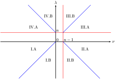
Figure 2.1: Octants of the parameter space

The results are graphically represented in Figures 2.1–2.4. The large and the small rectangles stands for the reducible principal series representations $I(i),J(j)$ of the large group $G$ and the small group $G^{\prime}$ respectively. The rectangles are located in the octants of the parameter space $(\lambda,\nu)$ determined by the conditions on $(i,j)$.

The subrectangles at the bottom represents the irreducible subrepresentation; a small rectangle represents a finite-dimensional subquotient module, a large rectangle an infinite-dimensional subquotient.

A colored green subrectangle is the subrepresentation which is contained in the kernel of the operator of the symmetry breaking operator $\widetilde{\mathbb{A}}_{i,j}$, and a white upper rectangle implies the image of the symmetry breaking operator $\widetilde{\mathbb{A}}_{i,j}$ is contained in the irreducible subrepresentation.

Suppose first that $(i,j)\in{\mathcal{L}}$ is contained in I.A. Both representations $I(i)$ and $J(j)$ have finite-dimensional subrepresentations $F(-i)$ and $F(-j)$ respectively. Since $-j>-i$ the representation $F(-j)$ is not a summand $F(-i)_{|G^{\prime}}$ by Proposition 2.3, and therefore the finite-dimensional subrepresentation $F(-i)$ is in the kernel of the symmetry breaking operator $\widetilde{\mathbb{A}}_{i,j}$. On the other hand, by Theorem 1.6, we have

$$\widetilde{\mathbb{T}}_{{n-1-j}}\circ\widetilde{\mathbb{A}}_{i,n-1-j}=\frac{\pi^{\frac{n-1}{2}}}{\Gamma(n-1-j)}\widetilde{\mathbb{A}}_{i,j},$$

which implies that the image of the nontrivial symmetry breaking operator $\widetilde{\mathbb{A}}_{i,j}$ is the finite-dimensional subrepresentation $F(-j)$ or zero. Since $\widetilde{\mathbb{A}}_{i,j}\neq 0$ by Theorem 1.5, the image is in fact $F(-j)$.

Suppose now that $(i,j)\in{\mathcal{L}}$ is contained in II.A. The representation $I(i)$ has a finite-dimensional subrepresentation $F(-i)$, and $J(j)$ has a finite-dimensional quotient $F(j-n+1)$. The image of $F(-i)$ under the symmetry breaking operator $\widetilde{\mathbb{A}}_{i,j}$ is finite-dimensional or zero. Since $J(j)$ has no finite-dimensional subrepresentation, the finite-dimensional subrepresentation $F(-i)$ must be in the kernel of the symmetry breaking operator $\widetilde{\mathbb{A}}_{i,j}$. By Theorems 1.5 and 1.6, we have

$$\widetilde{\mathbb{T}}_{{j}}\circ\widetilde{\mathbb{A}}_{i,j}=\frac{\pi^{\frac{n-1}{2}}}{\Gamma(j)}\widetilde{\mathbb{A}}_{i,n-1-j}\not=0.$$

Thus the image of $\widetilde{\mathbb{A}}_{i,n-1-j}$ is finite-dimensional, and therefore $\widetilde{\mathbb{A}}_{i,j}$ defines a surjective $({\mathfrak{g}},K)$-homomorphism $T(i)_{K}\to J(j)_{K^{\prime}}$.

Suppose that $(i,j)\in{\mathcal{L}}$ is contained in IV.A. The representation $I(i)$ has a finite-dimensional quotient $F(i-n)$, and $J(j)$ has a finite-dimensional subrepresentation $F(-j)$. The functional equation in Theorem 1.6 and the non-zero condition in Theorem 1.5 imply

$$\widetilde{\mathbb{A}}_{i,j}\circ\widetilde{\mathbb{T}}_{{n-i}}=\frac{\pi^{\frac{n}{2}}}{\Gamma(i)}\widetilde{\mathbb{A}}_{n-i,j}\not=0$$

Further, since $(n-i,j)$ is contained in I.A, the image of $T(i)$ under the symmetry breaking operator $\widetilde{\mathbb{A}}_{i,j}$ is the finite-dimensional representation $F(-j)$. Since $T(i)$ has a finite-codimension in $I(i)$, the image of $I(i)$ under the symmetry breaking operator $\widetilde{\mathbb{A}}_{i,j}$ is still finite-dimensional, hence is equal to the unique subrepresentation $F(-j)$ of $J(j)$.

Suppose that $(i,j)\in{\mathcal{L}}$ is contained in III.A. The representation $I(i)$ and $J(j)$ both have finite-dimensional quotients $F(i-n)$ and $F(j-n+1)$. Furthermore the multiplicity $m(I(i),J(j)))=1$ by Theorem 1.1. Again the spherical vector is not in the kernel of $\widetilde{\mathbb{A}}_{i,j}$, but its image is a spherical vector for $J(j)$ by Theorem 1.10, which in turn generates the underlying $({\mathfrak{g}}^{\prime},K^{\prime})$-module of $J(j)_{K^{\prime}}$. Hence the symmetry breaking operator $\widetilde{\mathbb{A}}_{i,j}$ is a surjective map from $I(i)_{K}$ to $J(j)_{K^{\prime}}$.

Figure 2.2 represents the results for the operator $\widetilde{\mathbb{A}}_{i,j}$ with $(i,j)\in{\mathcal{L}}$ in the four octants I.A, II.A, III.A, and IV.A discussed so far.

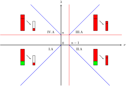
Figure 2.2: Image of $\widetilde{\mathbb{A}}_{i,j}$ with $(i,j)\in{\mathcal{L}}$

Suppose now that $(i,j)\in{\mathcal{L}}$ is contained in II.B. The representation $I(i)$ has a finite-dimensional subrepresentation and $J(j)$ has a finite-dimensional quotient. Furthermore we have $m(I(i),J(j))=1$ by Theorem 1.1. The image of a finite-dimensional $G^{\prime}$-invariant space of $I(i)$ under $\widetilde{\mathbb{A}}_{i,j}$ is finite-dimensional or zero. Since $J(j)$ has no finite-dimensional subrepresentation, the finite-dimensional subrepresentation $F(i)$ lies in the kernel of the symmetry breaking operator $\widetilde{\mathbb{A}}_{i,j}.$ Consider the functional equation from Theorem 1.6

$$\widetilde{\mathbb{T}}_{{j}}\circ\widetilde{\mathbb{A}}_{i,j}=\frac{\pi^{\frac{n-1}{2}}}{\Gamma(j)}\widetilde{\mathbb{A}}_{i,n-1-j}.$$

If $(i,j)\in\mathcal{L}_{odd}$ then the right-hand side is non-zero by Theorem 1.6 and thus $\widetilde{\mathbb{T}}_{{j}}\circ\widetilde{\mathbb{A}}_{i,j}\not=0$. In particular the image of $\widetilde{\mathbb{T}}_{{j}}\circ\widetilde{\mathbb{A}}_{i,j}$ is finite-dimensional. Thus the symmetry breaking operator $\widetilde{\mathbb{A}}_{i,j}$ must have a dense image, and therefore, induces a surjective $({\mathfrak{g}},K)$-homomorphism $I(i)_{K}\to J(j)_{K^{\prime}}$.
If $(i,j)\in\mathcal{L}_{even}$ then the symmetry breaking operator $\widetilde{\mathbb{A}}_{i,n-1-j}=0$ by Theorem 1.5. Hence the image of $\widetilde{\mathbb{A}}_{i,j}$ is contained in the subrepresentation $T(j-n+1)$ and thus induces a non-zero element in $\operatorname{Hom}_{G^{\prime}}(T(i),T(j-n+1))$.

Suppose now that $(i,j)\in{\mathcal{L}}$ is contained in IV.B. The representation $I(i)$ has a finite-dimensional quotient and $J(j)$ has a finite-dimensional subrepresentation. Furthermore the multiplicity $m(I(i),J(j))=1$. Consider the functional equation from Theorem 1.6

$$\widetilde{\mathbb{A}}_{i,j}\circ\widetilde{\mathbb{T}}_{{n-i}}=\frac{\pi^{\frac{n}{2}}}{\Gamma(i)}\widetilde{\mathbb{A}}_{n-i,j}$$

If $(i,j)\in\mathcal{L}_{odd}$ then $\frac{\pi^{\frac{n}{2}}}{\Gamma(i)}\widetilde{\mathbb{A}}_{n-i,j}\neq 0$ by Theorem 1.5. Hence the image $T(i-n)$ of the Knapp–Stein intertwining operator $\widetilde{\mathbb{T}}_{{n-i}}$ is not in the kernel of the symmetry breaking operator $\widetilde{\mathbb{A}}_{i,j}$. By the same argument as in IV.A, the image of the symmetry breaking operator is finite-dimensional, and thus it induces a nontrivial element in $\operatorname{Hom}_{G^{\prime}}(T(i-n)_{K},F(j))$.

If $(i,j)\in\mathcal{L}_{even}$ then $\widetilde{\mathbb{A}}_{n-i,j}=0$. Hence the image $T(i-n)$ of the Knapp–Stein intertwining operator $\widetilde{\mathbb{T}}_{{n-i}}$ for $G$ is in the kernel of the symmetry breaking operator $\widetilde{\mathbb{A}}_{i,j}$ and therefore it induces a non-zero operator in $\operatorname{Hom}_{G^{\prime}}(F(i-n),F(j))$.

Suppose now that $(i,j)\in{\mathcal{L}}$ is contained in III.B. The representation $I(i)$ and $J(j)$ have both finite-dimensional quotients. Furthermore we have $m(I(i),J(j))=1$ by Theorem 1.1. Consider the functional equation from Theorem 1.6

$$\widetilde{\mathbb{A}}_{i,j}\circ\widetilde{\mathbb{T}}_{{n-i}}=\frac{\pi^{\frac{n}{2}}}{\Gamma(i)}\widetilde{\mathbb{A}}_{n-i,j}.$$

It implies that the image $T(i-n)$ of the Knapp–Stein intertwining operator $\widetilde{\mathbb{T}}_{{n-i}}$ of $G$ is not in the kernel of $\widetilde{\mathbb{A}}_{i,j}$. Furthermore $\widetilde{\mathbb{A}}_{i,j}$ acts nontrivially on the spherical vector by Theorem 1.10, and its image is a cyclic vector in $J(j)$. Hence the symmetry breaking operator $\widetilde{\mathbb{A}}_{i,j}$ induces a surjective map from $I(i)_{K}$ to $J(j)_{K^{\prime}}$.

Remark 2.4.

If $(i,j)\in\mathcal{L}_{even}$, then the functional equation also implies that the image of $T(i-n)_{K}$ is $T^{\prime}(j-n+1)_{K^{\prime}}$.

Suppose now that $(i,j)\in{\mathcal{L}}$ is contained in I.B. The representations $I(i)$ and $J(j)$ have finite-dimensional subrepresentations $F(-i)$ and $F(-j)$, respectively.

If $(i,j)\in\mathcal{L}_{odd}$, then $m(I(i),J(j))=1$. The image of $\widetilde{\mathbb{A}}_{i,j}$ is finite-dimensional because

$$\widetilde{\mathbb{T}}_{{j}}\circ\widetilde{\mathbb{A}}_{i,j}=\frac{\pi^{\frac{n-1}{2}}}{\Gamma(j)}\widetilde{\mathbb{A}}_{i,n-1-j}=0.$$

Another functional equation

$$\widetilde{\mathbb{A}}_{i,j}\circ\widetilde{\mathbb{T}}_{{n-i}}=\frac{\pi^{\frac{n}{2}}}{\Gamma(i)}\widetilde{\mathbb{A}}_{n-i,j}=0$$

implies that the finite-dimensional representation $F(-i)$ is contained in the kernel of $\widetilde{\mathbb{A}}_{i,j}$ and so it induces a non-zero symmetry breaking operator in $\operatorname{Hom}_{G^{\prime}}(T(-i),F(-j))$.

If $(i,j)\in\mathcal{L}_{even}$, then $\widetilde{\mathbb{A}}_{i,j}=0$ by Theorem 1.5.

Figure 2.3 represents the results for $\widetilde{\mathbb{A}}_{i,j}$ in the 4 octants I.B, II.B, III.B, and IV.B for $(i,j)\in{\mathcal{L}}_{odd}$

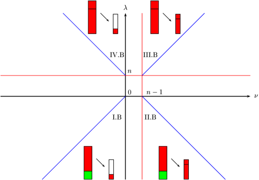
Figure 2.3: Image of $\widetilde{\mathbb{A}}_{i,j}$ with $(i,j)\in{\mathcal{L}}_{\operatorname{odd}}$

Similarly, Figure 2.4 represents the results for $\widetilde{\mathbb{A}}_{i,j}$ in the 4 octants for $(i,j)\in{\mathcal{L}}_{even}$

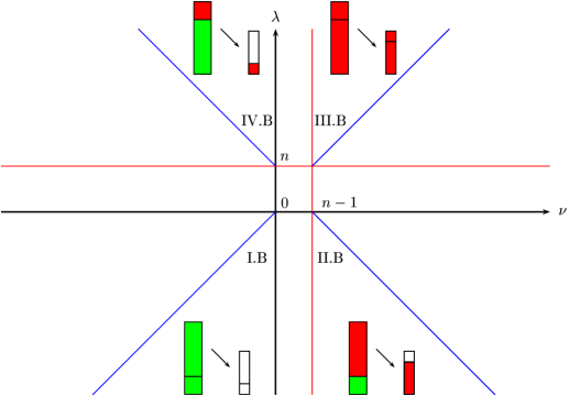
Figure 2.4: Image of $\widetilde{\mathbb{A}}_{i,j}$ with $(i,j)\in{\mathcal{L}}_{even}$

If $(i,j)\in L_{\operatorname{even}}$, namely, if $(i,j)\in{\mathcal{L}}_{even}$ with $i\leq j\leq 0$, then the multiplicity $m(I(i),J(j))=2$ and $H(i,j)$ is spanned by $\widetilde{\widetilde{{\mathbb{A}}}}_{i,j}$ and ${\tilde{{\mathbb{C}}}}_{i,j}$ by Theorem 1.9. The image of $\widetilde{\widetilde{{\mathbb{A}}}}_{i,j}$ is finite-dimensional and since the restriction to the finite-dimensional subrepresentation is nontrivial it induces an $G^{\prime}$-equivariant operator between the finite-dimensional representations $F(-i)$ and $F(-j)$. By Theorem 13.1 the image of $I(i)_{K}$ under ${\tilde{{\mathbb{C}}}}_{i,j}$ is equal to $J(-j)_{K^{\prime}}$ and the finite-dimensional representation is not in the kernel by Theorem 13.3 (5).

Figure 2.5 represents the results for the operators $\tilde{\tilde{\mathbb{A}}}_{i,j}$ and $\widetilde{\mathbb{C}}_{i,j}$ with $(i,j)\in{L}_{\operatorname{even}}$

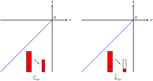
Figure 2.5: Images of $\tilde{\tilde{\mathbb{A}}}_{i,j}$ and $\widetilde{\mathbb{C}}_{i,j}$ with $(i,j)\in L_{\operatorname{even}}$

2.4 Multiplicities for composition factors

The following theorem generalizes the results by [29] for $G=GL(2,{\mathbb{C}})$ and $G^{\prime}=GL(2,{\mathbb{R}})$.

Theorem 2.5 (multiplicities for composition factors).

Let $i,j\in{\mathbb{N}}$.

1. Suppose that $i>j$.

   (1-a)  Assume $i\equiv j\mod 2$, namely, $(-i,-j)\in L_{\operatorname{even}}$. Then

   $$m(T(i),T(j))=1,\qquad m(T(i),F(j))=0,\qquad m(F(i),F(j))=1.$$

   (1-b)  Assume $i\equiv j+1\mod 2$, namely, $(-i,-j)\in L_{\operatorname{odd}}$. Then

   $$m(T(i),T(j))=0,\qquad m(T(i),F(j))=1,\qquad m(F(i),F(j))=0.$$

2. Suppose that $i<j$. Then

   $$m(T(i),T(j))=0,\quad m(T(i),F(j))=1,\quad m(F(i),F(j))=0.$$

Proof.

The discussion in Section 2.3 (see Figures 2.3 and 2.4) shows that our symmetry breaking operators induce

$$m(T(i),T(j))\not=0\ \mbox{ and }m(F(i),F(j))=1\ \mbox{ for }(-i,-j)\in L_{\operatorname{even}},$$

$$m(T(i),F(j))\not=0\quad\text{for }(-i,-j)\in L_{\operatorname{odd}},$$

and

$$m(T(i),F(j))\neq 0\quad\text{for }i<j.$$

Hence by [35] the multiplicities are one and it suffices to show that the multiplicities are zero in the remaining cases.

If $(-i,-j)\in L_{\operatorname{even}}$ and $m(T(i),F(j))\not=0$, then there would exist a nontrivial symmetry breaking operator $I(-i)\rightarrow J(-j)$ with image in the subrepresentation $F(-j)$ for which the finite-dimensional representation $F(i)$ is in the kernel. Since $F(i)$ is not in the kernel of $\widetilde{\widetilde{\mathbb{A}}}_{i,j}$ or $\widetilde{\mathbb{C}}_{i,j}$, this would imply that $m(I(i),J(j))>2$, contradicting Theorem 1.9.

We have already shown in Proposition 2.3 that $m(F(i),F(j))=0$ if $(-i,-j)\in L_{\operatorname{odd}}$ or $i<j$. Alternatively, this can be proved as follows: Suppose that $(-i,-j)\in L_{\operatorname{odd}}$ or $i<j$. If $m(F(i),F(j))\not=0$, then we would obtain an additional symmetry breaking operator for $(n+i,-j)$ in the octant IV.A or IV.B, contradicting Theorem 1.9.

Now suppose that $(-i,-j)\in L_{\operatorname{odd}}$ or $i<j$. Similarly, if $m(T(i),T(j))\not=0$, then we would obtain an additional symmetry breaking operator for $(\lambda,\nu)=(-i,n-1+j)$ in the octant II.A or II.B, contradicting Theorem 1.9. ∎

The following theorem determines the multiplicity from principal series representations $I(\lambda)$ of $G$ (not necessarily irreducible) to the irreducible representations $F(j)$ and $T(j)$ of $G^{\prime}$:

Theorem 2.6.

Suppose $j\in{\mathbb{N}}$.

1. $m(I(\lambda),F(j))=1\quad\quad\text{for all }\,\,\lambda\in{\mathbb{C}}.$

2. $m(I(\lambda),T(j))=\begin{cases}1\quad&\text{if }\,\,\lambda+j\in-2{\mathbb{N}},\\ 0\quad&\text{if }\,\,\lambda+j\not\in-2{\mathbb{N}}.\end{cases}$

It is noteworthy that there exist non-trivial symmetry breaking operators to the finite-dimensional representations $F(j)$, whereas there do not exist to the infinite-dimensional irreducible representations $T(j)$ for generic parameter $\lambda$.

Proof of Theorem 2.6.

1)  For any $\lambda\in{\mathbb{C}}$ and $\nu=-j\in{\mathbb{N}}$, we have

$$0\neq\tilde{\tilde{\mathbb{A}}}_{\lambda,\nu}\in\operatorname{Hom}_{G^{\prime}}(I(\lambda),J(\nu))$$

by Proposition 8.7, and $\operatorname{Image}\tilde{\tilde{\mathbb{A}}}_{\lambda,\nu}=F(j)$ by Theorem 13.1 (2) (see also Theorem 1.11). Hence $m(I(\lambda),F(j))\geq 1$.

On the other hand, in view of the inclusion relation for $\nu=-j\in{\mathbb{N}}$

$$\operatorname{Hom}_{G^{\prime}}(I(\lambda),F(j))\subset\operatorname{Hom}_{G^{\prime}}(I(\lambda),J(\nu)),$$

we have $m(I(\lambda),F(j))\leq 1$ if $(\lambda,-j)\notin L_{\operatorname{even}}$ by Theorem 1.1.

Suppose now that $(\lambda,-j)\in L_{\operatorname{even}}$. Then $\operatorname{Hom}_{G^{\prime}}(I(\lambda),J(\nu))$ is spanned by $\tilde{\tilde{\mathbb{A}}}_{\lambda,\nu}$ and $\widetilde{\mathbb{C}}_{\lambda,\nu}$ with $\nu=-j$ by Theorem 1.9, but $\operatorname{Image}\widetilde{\mathbb{C}}_{\lambda,\nu}\supsetneqq F(j)$ by Theorem 1.11 (1). Hence $m(I(\lambda),F(j))\leq 1$ if $(\lambda,-j)\in L_{\operatorname{even}}$, too. Thus the first statement is proved.

2) For $\nu=m+j$, we have from Theorem 1.1 and (2.11),

$$m(I(\lambda),T(j))\leq m(I(\lambda),J(\nu))=1$$

for any $\lambda\in{\mathbb{C}}$.

On the other hand, if $\lambda+j\in-2{\mathbb{N}}$, then $\widetilde{\mathbb{A}}_{\lambda,\nu}\neq 0$ by Theorem 1.5 and $\operatorname{Image}\widetilde{\mathbb{A}}_{\lambda,\nu}\subset T(j)$ by Theorem 13.2 (2). Hence $m(I(\lambda),T(j))=1$ for $\lambda+j\in-2{\mathbb{N}}$.

Finally suppose $\lambda+j\not\in-2{\mathbb{N}}$. Then $\widetilde{\mathbb{A}}_{\lambda,\nu}$ is nonzero but $\operatorname{Image}\widetilde{\mathbb{A}}_{\lambda,\nu}$ is not contained in $T(j)$ by Theorem 13.2 (2). If $m(I(\lambda),T(j))\neq 0$, then we would obtain an additional symmetry breaking operator from $I(\lambda)$ to $J(\nu)$ for $\nu=m+j$, contradicting Theorem 1.1. Thus Theorem 2.6 is proved. ∎

3 Symmetry breaking operators

Although our main object is the pair of groups $(G,G^{\prime})=(O(n+1,1),O(n,1))$, the techniques of this article are actually directed at the more general problems of determining symmetry breaking operators. In this chapter we study the distribution kernels of symmetry breaking operators between induced representations of a Lie group $G$ and its subgroup $G^{\prime}$ from their subgroups $H$ and $H^{\prime}$, respectively, in the general setting, and introduce the notion of regular (singular, or differential) symmetry breaking operators in terms of the double coset $H^{\prime}\backslash G/H$. When these representations are (possibly, degenerate) principal series representations of reductive groups, we discuss a reduction to the analysis on an open Bruhat cell under some mild condition.

3.1 Restriction of representations and symmetry breaking operators

Let $H$ be a closed subgroup of $G$. Given a finite-dimensional representation $\lambda:H\to GL_{\mathbb{C}}(V)$, we define the homogeneous vector bundle

$$\mathcal{V}_{X}\equiv\mathcal{V}:=G\times_{H}V$$

over the homogeneous space $X:=G/H$. The group $G$ acts continuously on the space $C^{\infty}(X,\mathcal{V})$ of smooth sections endowed with the natural Fréchet topology.

Suppose that $G^{\prime}$ is a subgroup of $G$, and $H^{\prime}$ is a closed subgroup of $G^{\prime}$. Similarly, given a finite-dimensional representation $\nu:H^{\prime}\to GL_{\mathbb{C}}(W)$, we have a continuous representation of $G^{\prime}$ on the Fréchet space $C^{\infty}(Y,{\mathcal{W}})$, where $\mathcal{W}:=G^{\prime}\times_{H^{\prime}}W$ is the homogeneous vector bundle over $Y:=G^{\prime}/H^{\prime}$.

We denote by

$$H(\lambda,\nu):=\operatorname{Hom}_{G^{\prime}}(C^{\infty}(X,\mathcal{V}),C^{\infty}(Y,\mathcal{W}))$$

the space of continuous $G^{\prime}$-homomorphisms, i.e., symmetry breaking operators.

3.2 Distribution kernels of symmetry breaking operators

By the Schwartz kernel theorem a continuous linear operator $T:C^{\infty}(X,{\mathcal{V}})\to C^{\infty}(Y,{\mathcal{W}})$ is given by a distribution kernel. In this section, we analyze the kernels of the symmetry breaking operators.

Let $\mathbb{C}_{2\rho}$ be the one-dimensional representation of $H$ defined by

$$h\mapsto|\det(\operatorname{Ad}_{G/H}(h):\mathfrak{g}/\mathfrak{h}\to\mathfrak{g}/\mathfrak{h})|^{-1}.$$

The bundle of volume densities $\Omega_{X}$ of $X=G/H$ is given as a $G$-homogeneous line bundle $\Omega_{X}\simeq G\times_{H}\mathbb{C}_{2\rho}$. Then the dualizing bundle of $\mathcal{V}$ is given, as a homogeneous vector bundle, by

$$\mathcal{V}^{*}:=(G\times_{H}V^{\vee})\otimes\Omega_{X}\simeq G\times_{H}(V^{\vee}\otimes\mathbb{C}_{2\rho}),$$

where $V^{\vee}$ denotes the contragredient representation of $V$.

In what follows $\mathcal{D}^{\prime}(X,\mathcal{V}^{*})$ denotes the space of $\mathcal{V}^{*}$-valued distributions.

Remark 3.1.

We shall regard distributions as generalized functions à la Gelfand [6] (or a special case of hyperfunctions à la Sato) rather than continuous linear forms on $C_{c}^{\infty}(X,\mathcal{V})$. The advantage of this convention is that the formula of the $G$-action (and of the infinitesimal action of the Lie algebra ${\mathfrak{g}}$) on ${\mathcal{D}}^{\prime}(X,{\mathcal{V}}^{\ast})$ is the same with that of $C^{\infty}(X,{\mathcal{V}}^{\ast})$.

Proposition 3.2.

Suppose that $G^{\prime}$ and $H$ are closed subgroups of $G$ and that $H^{\prime}$ is a closed subgroup of $G^{\prime}$.

1. There is a natural injective map:

   $$\operatorname{Hom}_{G^{\prime}}(C^{\infty}(X,\mathcal{V}),C^{\infty}(Y,\mathcal{W}))\hookrightarrow(\mathcal{D}^{\prime}(X,\mathcal{V}^{*})\otimes W)^{\Delta(H^{\prime})},\,\,T\mapsto K_{T}.$$ (3.1)

   Here $H^{\prime}$ acts diagonally via the action of $G\times H^{\prime}$ on $\mathcal{D}^{\prime}(X,\mathcal{V}^{*})\otimes W$.

2. If $H$ is cocompact in $G$ (e.g. a parabolic subgroup of $G$), then (3.1) is a bijection.

Proof.

1)  Any continuous operator $T:C^{\infty}(X,\mathcal{V})\to C^{\infty}(Y,\mathcal{W})$ is given uniquely by a distribution kernel $K_{T}\in\mathcal{D}^{\prime}(X\times Y,\mathcal{V}^{*}\boxtimes\mathcal{W})$ owing to the Schwartz kernel theorem. If $T$ intertwines with the $G^{\prime}$-action, then the distribution $K_{T}$ is invariant under the diagonal action of $G^{\prime}$, namely, $K_{T}(g^{\prime}\cdot,g^{\prime}\cdot)=K_{T}(\cdot,\cdot)$ for any $g^{\prime}\in G^{\prime}$. In turn, the multiplication map

$$m:G\times G^{\prime}\to G,\ (g,g^{\prime})\mapsto(g^{\prime})^{-1}g$$

induces a natural bijection

$$m^{\ast}:\mathcal{D}^{\prime}(X\times Y,\mathcal{V}^{*}\boxtimes\mathcal{W})^{\Delta(G^{\prime})}\overset{\sim}{\leftarrow}(\mathcal{D}^{\prime}(X,\mathcal{V}^{*})\otimes W)^{\Delta(H^{\prime})}.$$ (3.2)

Thus we have proved the first statement.

2) Conversely, any distribution $K\in\mathcal{D}^{\prime}(X\times Y,\mathcal{V}^{*}\boxtimes\mathcal{W})$ induces a linear map

$$T:C^{\infty}(X,\mathcal{V})\to\mathcal{D}^{\prime}(Y,\mathcal{W})$$

if $X$ is compact. Further, if $K$ is $G^{\prime}$-invariant via the diagonal action, then it follows from (3.2) that $Tf$ is a smooth section of the bundle ${\mathcal{W}}\to Y$ for any $f\in C^{\infty}(X,\mathcal{V})$ and $T:C^{\infty}(X,\mathcal{V})\to C^{\infty}(Y,\mathcal{W})$ is a continuous $G^{\prime}$-homomorphism. Therefore the injective morphism (3.1) is also surjective. ∎

In Proposition 3.2, the support of $K_{T}$ is an $H^{\prime}$–invariant closed subset in $G/H$. Thus the closed $H^{\prime}$–invariant sets define a coarse invariant of a symmetry breaking operator:

$$\operatorname{Hom}_{G^{\prime}}(C^{\infty}(X,\mathcal{V}),C^{\infty}(Y,\mathcal{W}))\to\{\text{$H^{\prime}$-invariant closed subsets in $G/H$}\},$$ (3.3)

$$T\mapsto\operatorname{Supp}K_{T}.$$

In rest of the chapter we assume that:

$$H^{\prime} G/H$$ has an open orbit on . (3.4)

Definition 3.3.

Let $U_{i}$ ($i=1,2,\cdots$) be the totality of $H^{\prime}$-open orbits on $X=G/H$. A non-zero $G^{\prime}$-intertwining operator $T:C^{\infty}(X,{\mathcal{V}})\to C^{\infty}(Y,{\mathcal{W}})$ is regular if $\operatorname{Supp}K_{T}$ contains at least one open orbit $U_{i}$. We say $T$ is singular if $T$ is not regular, namely, if $\operatorname{Supp}K_{T}\subset X-\cup_{i}U_{i}$.

We write $H(\lambda,\nu)_{\operatorname{sing}}$ for the space of singular symmetry breaking operators.

Example 3.4.

1. (Knapp–Stein intertwining operators). Here $G=G^{\prime}$ and $H=H^{\prime}$ is a minimal parabolic subgroup $P$ of $G$ and $W$ and $V$ are irreducible representations of $P$. The Bruhat decomposition determines the orbits of $P$ on $G/P$. Hence we have exactly one open orbit corresponding to the longest element in the Weyl group. Thus the intertwining operator corresponding to the longest element of the Weyl group is regular for generic parameter. See [15].

2. (Poisson transforms for symmetric spaces). Here $G=G^{\prime}$, $H$ is a minimal parabolic subgroup $P$ of $G$, $H^{\prime}$ is a maximal compact subgroup $K$ of $G$, $V$ is a one-dimensional representations of $P$ and $W$ is the trivial one-dimensional representation, see [10]. Since $KP=G$, the assumption (3.4) is satisfied and the Poisson transform is a regular symmetry breaking operator. More generally, if $(G,H^{\prime})$ is a reductive symmetric pair, then $H^{\prime}$ has finitely many open orbits on $G/P$ and a similar integral transform (Poisson transform for the reductive symmetric space $G/H^{\prime}$) can be defined and has a meromorphic continuation with respect to the parameter of the one-dimensional representations of $P$ for each $H^{\prime}$-open orbit, see [30].

3. (Fourier transform for symmetric spaces). If we switch the role of $H$ and $H^{\prime}$ in 2), the integral transforms can be defined as the adjoint of the Poisson transforms, and are said to be the Fourier transforms for the Riemannian symmetric space $G/K$ [10] and the reductive symmetric space $G/H^{\prime}$.

4. (invariant trilinear form). Let $P_{1}$ be a parabolic subgroup of a reductive group $G_{1}$, $G=G_{1}\times G_{1}$, $H=P_{1}\times P_{1}$, $G^{\prime}=\operatorname{diag}(G_{1})$, and $H^{\prime}=\operatorname{diag}(G^{\prime})$. The study of symmetry breaking operators is equivalent to that of invariant trilinear forms on $\pi_{\lambda_{1}}\otimes\pi_{\lambda_{2}}\otimes\pi_{\lambda_{3}}$ where $\pi_{\lambda_{i}}=\operatorname{Ind}_{P_{1}}^{G_{1}}(\lambda_{i})$ $(i=1,2,3)$. See [1] for the construction of invariant trilinear forms and explicit formula of generalized Bernstein–Reznikov integrals in some examples where (3.4) is satisfied.

5. (Jantzen–Zuckerman translation functor).  Here $G=G^{\prime}\times G^{\prime}$ and $G^{\prime}$ is a diagonally embedded subgroup of $G$. We start with a brief review of (abstract) translation functors. Let $Z({\mathfrak{g}})$ be the center of the enveloping algebra $U({\mathfrak{g}})$. Given a smooth admissible, irreducible representation $\pi$ and a finite-dimensional representation $F$ of $G^{\prime}$, we consider the restriction of the outer tensor product representation of $G$ to $G^{\prime}$:

   $$\pi\otimes F=(\pi\boxtimes F)|_{G^{\prime}}.$$

   Since $\pi\otimes F$ is an admissible representation of finite length, the projection $\operatorname{pr}_{\chi}$ to the component of a generalized infinitesimal character $\chi$ is well-defined. The functor $\pi\rightsquigarrow\operatorname{pr}_{\chi}(\pi\otimes F)$ is called a translation functor. Geometrically if $\pi$ is an induced representation $C^{\infty}(G/P,{\mathcal{V}})$ from a finite-dimensional representation $V$ of $P$, then the translation functor is a symmetry breaking operator

   $$C^{\infty}(G/P,{\mathcal{V}})\otimes F\to C^{\infty}(G/P,{\mathcal{W}}),$$

   where ${\mathcal{W}}=G\times_{P}W$ and $W$ is a certain $P$-subquotient (determined by $\chi$) of the finite-dimensional representation $(V\otimes F)|_{P}$.

If $T$ is a symmetry breaking operator, the restriction of the distribution kernel $K_{T}$ to open $H^{\prime}$-orbits $U_{i}$ is a regular function. By using this, we obtain an upper bound of linearly independent, regular symmetry breaking operators as follows: We take $x_{i}\in U_{i}$, and denote by $M_{i}^{\prime}$ the stabilizer of $H^{\prime}$ at $x_{i}$, and thus we have $H^{\prime}/M_{i}^{\prime}\simeq U_{i}$.

Proposition 3.5.

Assume (3.4). Then

$$\dim H(\lambda,\nu)/H(\lambda,\nu)_{\operatorname{sing}}\leq\sum_{i}\dim\operatorname{Hom}_{M_{i}^{\prime}}(\lambda|_{M_{i}^{\prime}},\nu|_{M_{i}^{\prime}}).$$

Proof.

Since the distribution kernel $K_{T}$ is $H^{\prime}$-invariant, the restriction of $K_{T}$ to each open $H^{\prime}$-orbit $U_{i}$ is a regular function which is determined uniquely by its value at a single point, e.g., $K_{T}(x_{i})$ at $x_{i}$. Further, $K_{T}(x_{i})\in\operatorname{Hom}_{\mathbb{C}}(V,W)$ inherits the $M_{i}^{\prime}$-invariance from the $H^{\prime}$-invariance of $K_{T}$, namely, we have $K_{T}(x_{i})\in\operatorname{Hom}_{M^{\prime}_{i}}(\lambda|_{M^{\prime}_{i}},\nu|_{M^{\prime}_{i}})$. ∎

Corollary 3.6.

If $\operatorname{Hom}_{M^{\prime}_{i}}(\lambda|_{M^{\prime}_{i}},\nu|_{M^{\prime}_{i}})=0$ for all $i$, then any $G^{\prime}$-intertwining operator $T\in H(\lambda,\nu)$ is singular.

Remark 3.7.

Even if $\operatorname{Hom}_{M^{\prime}_{i}}(\lambda|_{M^{\prime}_{i}},\nu|_{M^{\prime}_{i}})=0$, there may exist a nonzero singular symmetry breaking operator $I(\lambda)\to J(\nu)$ for specific parameters $\lambda$ and $\nu$.

Corollary 3.8.

Assume both $V$ and $W$ are one-dimensional. If there are $N$ open $H^{\prime}$-orbits on $G/H$, then

$$\dim H(\lambda,\nu)/H(\lambda,\nu)_{\operatorname{sing}}\leq N.$$

In particular, if there exists a unique $H^{\prime}$-orbit on $G/H$, then

$$\dim H(\lambda,\nu)/H(\lambda,\nu)_{\operatorname{sing}}\leq 1.$$

Remark 3.9.

If $H$ is a minimal parabolic subgroup of $G$ then $N$ does not exceed the cardinality of the little Weyl group of $G$ for any subgroup $H^{\prime}$ of $G$ ([25, Corollary E]).

The role of the assumption (3.4) is illuminated by the following:

Proposition 3.10.

Suppose $G$ is an algebraic group, and the subgroups $H$ and $H^{\prime}$ are defined algebraically. If (3.4) is not fulfilled, then for any algebraic finite-dimensional representation $V$ of $H$, there exists a finite-dimensional representation $W$ of $H^{\prime}$ such that

$$\dim H(\lambda,\nu)=\infty.$$

Proof.

The argument is similar to that of [25, Theorem 3.1], and we omit the proof. ∎

In the case $(G,G^{\prime})$ is a reductive symmetric pair, and $H$, $H^{\prime}$ are minimal parabolic subgroups of $G$, $G^{\prime}$, respectively, the pairs $(G,G^{\prime})$ satisfying (3.4) were classified recently [20].

3.3 Differential intertwining operators

Suppose further that

$$H^{\prime}\subset H\cap G^{\prime}.$$ (3.5)

Then we have a natural homomorphism $\iota:Y\rightarrow X$, which is $G^{\prime}$-equivariant. Using the morphism $\iota$, we can define the notion of differential operators in a wider sense than the usual:

Definition 3.11.

We say a continuous linear operator $T:C^{\infty}(X,{\mathcal{V}})\to C^{\infty}(Y,{\mathcal{W}})$ is a differential operator if

$$\iota({\operatorname{Supp}}(Tf))\subset{\operatorname{Supp}}f\quad\text{for any }f\in C^{\infty}(X,{\mathcal{V}}).$$

In the case $H^{\prime}=H\cap G^{\prime}$, the morphism $\iota$ is injective, and a differential operator $T$ in the sense of Definition 3.11 is locally of the form

$$T=\sum_{(\alpha,\beta)\in{\mathbb{N}}^{\dim X}}g_{\alpha\beta}(y)\frac{\partial^{|\alpha|+|\beta|}}{\partial y^{\alpha}\partial z^{\beta}}$$

where $g_{\alpha\beta}(y)$ are $\operatorname{Hom}(V,W)$-valued smooth functions on $Y$, and the local coordinates $\{(y_{i},z_{i})\}$ on $X$ are chosen in such a way that $\{y_{i}\}$ form an atlas on $Y$.

We denote by

$$H(\lambda,\nu)_{\rm{diff}}\equiv\operatorname{Diff}_{G^{\prime}}(\mathcal{V}_{X},\mathcal{W}_{Y}),$$

a subspace of $H(\lambda,\nu)\equiv\operatorname{Hom}_{G^{\prime}}(C^{\infty}(X,\mathcal{V}),C^{\infty}(Y,\mathcal{W}))$ consisting of $G^{\prime}$-intertwining differential operators.

It is widely known that, when $G=G^{\prime}$ and $X=Y$, holomorphic $G$-equivariant differential operators between holomorphic homogeneous bundles over the complex flag variety of a complex reductive Lie group $G$ are dual to $\mathfrak{g}$-homomorphisms between generalized Verma modules (e.g., [9]). The duality can be extended to our more general situation where two homogeneous bundles are defined over two different base spaces $\iota:Y\rightarrow X$. In order to give a precise statement, we need to take the disconnectedness of $H$ into account (see Remark 3.13). For this, we regard the generalized Verma module

$$\operatorname{ind}_{\mathfrak{h}_{\mathbb{C}}}^{\mathfrak{g}_{\mathbb{C}}}(V)=U(\mathfrak{g}_{\mathbb{C}})\otimes_{U(\mathfrak{h}_{\mathbb{C}})}V$$

as a $(\mathfrak{g},H)$-module where $V$ is an $H$-module. Here the $H$-action on $\operatorname{ind}_{\mathfrak{h}_{\mathbb{C}}}^{\mathfrak{g}_{\mathbb{C}}}(V)$ is induced from the diagonal action of $H$ on $U(\mathfrak{g}_{\mathbb{C}})\otimes_{\mathbb{C}}V$. Likewise, $\operatorname{ind}_{\mathfrak{h}^{\prime}_{\mathbb{C}}}^{\mathfrak{g}^{\prime}_{\mathbb{C}}}(W^{\vee})$ is a $(\mathfrak{g}^{\prime},H^{\prime})$-module if $W$ is an $H^{\prime}$-module. We then have:

Fact 3.12 (see [26, Theorem 2.7]).

Suppose $H^{\prime}\subset H\cap G^{\prime}$.

1. $T\in\operatorname{Hom}_{G^{\prime}}(C^{\infty}(X,{\mathcal{V}}),C^{\infty}(Y,{\mathcal{W}}))$ is a differential operator if and only if $\operatorname{Supp}K_{T}=\{eH\}$ in $G/H$.

2. There is a natural bijection:

   $$\operatorname{Hom}_{(\mathfrak{g}^{\prime},H^{\prime})}(\operatorname{ind}_{\mathfrak{h}^{\prime}_{\mathbb{C}}}^{\mathfrak{g}^{\prime}_{\mathbb{C}}}(W^{\vee}),\operatorname{ind}_{\mathfrak{h}_{\mathbb{C}}}^{\mathfrak{g}_{\mathbb{C}}}(V^{\vee}))\overset{\sim}{\to}\operatorname{Diff}_{G^{\prime}}(\mathcal{V}_{X},\mathcal{W}_{Y}).$$

Remark 3.13.

The disconnectedness of $H^{\prime}$ affects the dimension of the space of covariant differential operators. We will give an example of this in the case of Juhl’s operators in Section 10.2.

When (3.4) and (3.5) are satisfied, we have the following inclusion relation:

$$H(\lambda,\nu)\supset H(\lambda,\nu)_{\operatorname{sing}}\supset H(\lambda,\nu)_{\operatorname{diff}}.$$ (3.6)

This filtration will be used in the classification of the symmetry breaking operators in the later chapters (see Section 11.2, for instance).

3.4 Smooth representations and intertwining operators

Suppose that $G$ is a real reductive linear Lie group. In this section we review quickly the notion of Harish-Chandra modules and the Casselman–Wallach theory of Fréchet globalization, and show a closed range property of intertwining operators (Proposition 3.15 below).

We fix a maximal compact subgroup $K$ of $G$. We may and do realize $G$ as a closed subgroup of $GL(n,{\mathbb{R}})$ for some $n$ such that $g\in G$ if and only if ${}^{t}g^{-1}\in G$ and $K=O(n)\cap G$. For $g\in G$ we define a map $\|\cdot\|:G\to{\mathbb{R}}$ by

$$\|g\|:=\|g\oplus{}^{t}g^{-1}\|_{\operatorname{op}}$$

where $\|\,\|_{\operatorname{op}}$ is the operator norm of $M(2n,{\mathbb{R}})$.

Let ${\mathcal{HC}}$ denote the category of Harish-Chandra modules where the objects are $({\mathfrak{g}},K)$-modules of finite length, and the morphisms are $({\mathfrak{g}},K)$-homomorphisms.

A continuous representation $\pi$ of $G$ on a Fréchet space $U$ is said to be of moderate growth if for each continuous semi-norm $|\cdot|$ on $U$ there exist a continuous semi-norm $|\cdot|^{\prime}$ on $U$ and $d\in{\mathbb{R}}$ such that

$$|\pi(g)u|\leq\|g\|^{d}|u|^{\prime}\quad\text{for }g\in G,u\in U.$$

Suppose $(\pi,{\mathcal{H}})$ is a continuous representation of $G$ on a Banach space ${\mathcal{H}}$. A vector $v\in{\mathcal{H}}$ is said to be smooth if the map $G\to{\mathcal{H}}$, $g\mapsto\pi(g)v$ is of $C^{\infty}$-class. Let ${\mathcal{H}}^{\infty}$ denote the space of smooth vectors of the representation $(\pi,{\mathcal{H}})$. Then ${\mathcal{H}}^{\infty}$ carries a Fréchet topology with a family of semi-norms $\|v\|_{i_{1}\cdots i_{k}}:=\|d\pi(X_{i_{1}})\cdots d\pi(X_{i_{k}})v\|$. Here $\{X_{1},\cdots,X_{n}\}$ is a basis of ${\mathfrak{g}}$. Then ${\mathcal{H}}^{\infty}$ is a $G$-invariant subspace of ${\mathcal{H}}$, and $(\pi,{\mathcal{H}}^{\infty})$ is a continuous Fréchet representation of $G$.

We collect some basic properties ([39, Lemma 11.5.1, Theorem 11.6.7]):

Fact 3.14.

1) If $(\pi,{\mathcal{H}})$ is a Banach representation, then $(\pi,{\mathcal{H}}^{\infty})$ has moderate growth.

2) Let $U_{1},U_{2}$ be continuous representations of $G$ having moderate growth such that the underlying $({\mathfrak{g}},K)$-modules $(U_{1})_{K},(U_{2})_{K}\in{\mathcal{HC}}$. If $T:(U_{1})_{K}\to(U_{2})_{K}$ is a $({\mathfrak{g}},K)$-homomorphism, then $T$ extends to a continuous $G$-intertwining operator $\overline{T}:U_{1}\to U_{2}$, with closed image that is a topological summand of $U_{2}$.

Let $P$, $P^{\prime}$ be parabolic subgroups of $G$, and ${\mathcal{V}}$, ${\mathcal{W}}$ the $G$-equivariant vector bundles over the real flag varieties $X=G/P$, $Y=G/P^{\prime}$ associated to finite-dimensional representations of $V$, $W$ of $P$, $P^{\prime}$, respectively. (In the setting here, $G^{\prime}=G$ in the notation of the previous sections.)

Proposition 3.15 (closed range property).

If $T:C^{\infty}(X,{\mathcal{V}})_{K}\to C^{\infty}(Y,{\mathcal{W}})_{K}$ is a $({\mathfrak{g}},K)$-homomorphism, then $T$ lifts uniquely to a continuous $G$-intertwining operator $\overline{T}$ from $C^{\infty}(X,{\mathcal{V}})$ to $C^{\infty}(Y,{\mathcal{W}})$, and the image of $\overline{T}$ is closed in the Fréchet topology of $C^{\infty}(Y,{\mathcal{W}})$.

Proof of Proposition 3.15.

We fix a Hermitian inner product on every fiber ${\mathcal{V}}_{x}$ that depends smoothly on $x\in X$, and denote by $L^{2}(X,{\mathcal{V}})$ the Hilbert space of square integrable sections to the Hermitian vector bundle ${\mathcal{V}}\to X$. Then we have a continuous representation of $G$ on the Hilbert space $L^{2}(X,{\mathcal{V}})$, and the space $(L^{2}(X,{\mathcal{V}}))^{\infty}$ of smooth vectors is isomorphic to $C^{\infty}(X,{\mathcal{V}})$ as Fréchet spaces because $X$ is compact and $V$ is finite-dimensional. Therefore $C^{\infty}(X,{\mathcal{V}})$ has moderate growth by Fact 3.14 (1). Furthermore, the underlying $({\mathfrak{g}},K)$-module $C^{\infty}(X,{\mathcal{V}})_{K}$ is admissible and finitely generated because $P$ is parabolic subgroup of $G$ and $V$ is of finite length as a $P$-module. Likewise $C^{\infty}(Y,{\mathcal{W}})$ has moderate growth with $C^{\infty}(Y,{\mathcal{W}})_{K}\in{\mathcal{HC}}$. Now Proposition follows from Fact 3.14 (2). ∎

3.5 Symmetry breaking operators for principal series representations

From now on we assume that $X$ and $Y$ are real flag varieties of real reductive groups $G$ and $G^{\prime}$. Let $P=MAN$ and $P^{\prime}=M^{\prime}A^{\prime}N^{\prime}$ be Langlands decompositions of parabolic subgroups $G$ and $G^{\prime}$, respectively, satisfying

$$M^{\prime}=M\cap G^{\prime},\ A^{\prime}=A\cap G^{\prime},\ N^{\prime}=N\cap G^{\prime},\ P^{\prime}=P\cap G^{\prime}.$$ (3.7)

This condition is fulfilled, for example, if the two parabolic subgroups $P$ and $P^{\prime}$ are defined by the same hyperbolic element of $G^{\prime}$, as in the setting of Section 2.1 that we shall work with in this article.

Let $P_{-}=MAN_{-}$ by the opposite parabolic subgroup, and ${\mathfrak{n}}_{-}$ the Lie algebra of $N_{-}$. The composition ${\mathfrak{n}}_{-}\hookrightarrow G\to G/P$, $Z\mapsto\exp Z\mapsto(\exp Z)P/P$ gives a parametrization of the open Bruhat cell of the real flag variety $X=G/P$. We shall regard ${\mathfrak{n}}_{-}$ simply as an open subset of $X=G/P$. We trivialize the dualizing vector bundle $\mathcal{V}^{*}\to X$ on the open Bruhat cell, and consider the restriction map

$$\mathcal{D}^{\prime}(X,\mathcal{V}^{*})\to\mathcal{D}^{\prime}({\mathfrak{n}}_{-})\otimes(V^{\vee}\otimes\mathbb{C}_{2\rho}).$$ (3.8)

The natural $G$-action on $\mathcal{D}^{\prime}(X,\mathcal{V}^{*})$ defines an infinitesimal action of the Lie algebra $\mathfrak{g}$ on $\mathcal{D}^{\prime}(U,\mathcal{V}^{*}|_{U})$ for any open subset $U$ of $X$. This induces a $\mathfrak{g}$-action on $\mathcal{D}^{\prime}({\mathfrak{n}}_{-})\otimes(V^{\vee}\otimes\mathbb{C}_{2\rho})$ so that (3.8) is a $\mathfrak{g}$-homomorphism. Likewise we let $MA$ act on $\mathcal{D}^{\prime}({\mathfrak{n}}_{-})\otimes(V^{\vee}\otimes\mathbb{C}_{2\rho})$ so that (3.8) is a $(\mathfrak{g},M^{\prime})$-map.

From now on we assume that

$$P^{\prime}N_{-}P=G.$$ (3.9)

Theorem 3.16.

Suppose (3.7) and (3.9) are satisfied. Then we have a natural bijection:

$$\operatorname{Hom}_{G^{\prime}}(C^{\infty}(G/P,\mathcal{V}),C^{\infty}(G^{\prime}/P^{\prime},\mathcal{W}))\simeq\mathcal{D}^{\prime}({\mathfrak{n}}_{-},\operatorname{Hom}_{\mathbb{C}}(V\otimes\mathbb{C}_{-2\rho},W))^{M^{\prime}A^{\prime},\mathfrak{n}}.$$

Remark 3.17.

The right-hand side may be regarded as $\operatorname{Hom}(V,W)$-valued distributions on ${\mathfrak{n}}_{-}$ satisfying certain $(M^{\prime}A^{\prime},\mathfrak{n}^{\prime})$-invariance conditions because $\dim\mathbb{C}_{-2\rho}=1$. In the main part of this article we treat the case

$$\dim V=\dim W=1$$

and we identify the distribution kernel $K_{T}$ with a distribution on ${\mathfrak{n}}_{-}$. We shall see that (3.9) is fulfilled for $(G,G^{\prime})=(O(n+1,1),O(n,1))$ in Corollary 5.5.

Proof of Theorem 3.16.

Since $P^{\prime}N_{-}P=G$, the restriction map (3.8) induces an injective morphism on $\Delta(P^{\prime})$-invariant distributions:

$$(\mathcal{D}^{\prime}(X,\mathcal{V}^{*})\otimes W)^{\Delta(P^{\prime})}\hookrightarrow(\mathcal{D}^{\prime}({\mathfrak{n}}_{-})\otimes(V^{\vee}\otimes\mathbb{C}_{2\rho})\otimes W)^{M^{\prime}A^{\prime},\mathfrak{n}^{\prime}}.$$ (3.10)

Conversely, given a $K\in\mathcal{D}^{\prime}({\mathfrak{n}}_{-},\mathcal{V}^{*}|_{{\mathfrak{n}}_{-}})\otimes W$ we define for each $p^{\prime}\in P^{\prime}$

$$p^{\prime}\cdot K\in\mathcal{D}^{\prime}(p^{\prime}\cdot{\mathfrak{n}}_{-},\mathcal{V}^{*}|_{p^{\prime}\cdot{\mathfrak{n}}_{-}})\otimes W.$$

Then $p^{\prime}\cdot K=K$ on the intersection ${\mathfrak{n}}_{-}\cap p^{\prime}\cdot{\mathfrak{n}}_{-}$ if $T\in(\mathcal{D}^{\prime}({\mathfrak{n}}_{-})\otimes\operatorname{Hom}_{\mathbb{C}}(V\otimes\mathbb{C}_{-2\rho},W))^{M^{\prime}A^{\prime},\mathfrak{n}^{\prime}}$. This shows the surjectivity of the restriction map (3.10). Hence Theorem 3.16 follows from Proposition 3.2. ∎

3.6 Meromorphic continuation of symmetry breaking operators

In order to discuss the meromorphic continuation of symmetry breaking operators for principal series representations, we fix finite-dimensional representations

$$\sigma:M\rightarrow GL_{\mathbb{C}}(V)$$

and

$$\tau:M^{\prime}\rightarrow GL_{\mathbb{C}}(W).$$

For $\lambda\in\mathfrak{a}_{\mathbb{C}}^{*}$ and $\nu\in(\mathfrak{a}^{\prime}_{\mathbb{C}})^{*}$, we define representations $V_{\lambda}$ of $P$ and $W_{\nu}$ of $P^{\prime}$ by

$$P =MAN \ni me^{H}n \mapsto\sigma(m)e^{\lambda(H)} \in GL_{\mathbb{C}}(V)$$

$$P^{\prime} =M^{\prime}A^{\prime}N^{\prime} \ni m^{\prime}e^{H^{\prime}}n^{\prime} \mapsto\tau(m^{\prime})e^{\nu(H^{\prime})} \in GL_{\mathbb{C}}(W),$$

respectively. Here by abuse of notation, we use $\lambda$ and $\nu$ also as parameters of representation spaces of $P$ and $P^{\prime}$, respectively. (Later, we shall work with the case where $\sigma={\bf{1}}$ and $\tau={\bf{1}}$.) We then have homogeneous bundles

$$\mathcal{V}_{\lambda}:=G\times_{P}V_{\lambda}$$

and

$$\mathcal{W}_{\nu}:=G^{\prime}\times_{P^{\prime}}W_{\nu}$$

over the real flag varieties $G/P$ and $G^{\prime}/P^{\prime}$, respectively. Observe that the pull-back of the vector bundle ${\mathcal{V}}_{\lambda}$ via the $K$-diffeomorphism $K/M\overset{\sim}{\to}G/P$ is a $K$-homogeneous vector bundle ${\mathcal{V}}=K\times_{M}(\sigma,V)$. Similarly, the pull-back of the vector bundle ${\mathcal{W}}_{\nu}$ yields a $K^{\prime}$-homogeneous vector bundle ${\mathcal{W}}=K^{\prime}\times_{M^{\prime}}(\tau,W)$. Thus, even though the $G$-module $C^{\infty}(G/P,\mathcal{V}_{\lambda})$ and the $G^{\prime}$-module $C^{\infty}(G^{\prime}/P^{\prime},\mathcal{W}_{\nu})$ have complex parameters $\lambda\in\mathfrak{a}_{\mathbb{C}}^{*}$ and $\nu\in(\mathfrak{a}^{\prime}_{\mathbb{C}})^{*}$, respectively, but the spaces themselves can be defined independently of $\lambda$ and $\nu$ as Fréchet spaces via the isomorphisms

$$C^{\infty}(G/P,\mathcal{V}_{\lambda})\simeq C^{\infty}(K/M,{\mathcal{V}}),\ C^{\infty}(G^{\prime}/P^{\prime},\mathcal{W}_{\nu})\simeq C^{\infty}(K^{\prime}/M^{\prime},{\mathcal{W}}).$$ (3.11)

Thus, for a family of continuous $G^{\prime}$-homomorphisms $T_{\lambda,\nu}:C^{\infty}(G/P,\mathcal{V}_{\lambda})\to C^{\infty}(G^{\prime}/P^{\prime},\mathcal{W}_{\nu})$, we can define the holomorphic (or meromorphic) dependence on the complex parameter $(\lambda,\nu)$ via (3.11), namely, we call a continuous linear map $T_{\lambda,\nu}$ depends holomorphically/meromorphically on $(\lambda,\nu)$ if $T_{\lambda,\nu}(\varphi)$ depends holomorphically/meromorphically on $(\lambda,\nu)$ for any $\varphi\in C^{\infty}(K/M,{\mathcal{V}})$.

For a family of distributions $D_{\lambda,\nu}\in\mathcal{D}^{\prime}({\mathfrak{n}}_{-},\operatorname{Hom}(V,W))$, we say $D_{\lambda,\nu}$ depends holomorphically/meromorphically on the parameter $(\lambda,\nu)\in\Omega$ if for every test function $F\in C^{\infty}({\mathfrak{n}}_{-},V)$ the function $D_{\lambda,\nu}(F)$ depends holomorphically/meromorphically on $(\lambda,\nu)$.

The following proposition asserts that the existence of holomorphic/meromorphic continuation of symmetry breaking operators is determined only by that of distribution kernels on the open Bruhat cell under a mild assumption.

Proposition 3.18.

Assume (3.7) and (3.9) are satisfied. Let $\Omega^{\prime}\subset\Omega$ be two open domains in $\mathfrak{a}_{\mathbb{C}}^{*}\times(\mathfrak{a}^{\prime}_{\mathbb{C}})^{*}$. Suppose we are given a family of continuous $G^{\prime}$-homomorphisms

$$T_{\lambda,\nu}:C^{\infty}(G/P,\mathcal{V}_{\lambda})\to C^{\infty}(G^{\prime}/P^{\prime},\mathcal{W}_{\nu})$$

for $(\lambda,\nu)\in\Omega^{\prime}$. Denote by $K_{\lambda,\nu}$ the restriction of the distribution kernel to the open Bruhat cell and suppose that $K_{\lambda,\nu}$ depends holomorphically on $(\lambda,\nu)\in\Omega^{\prime}$. We assume

$$\text{$K_{\lambda,\nu}$ extends holomorphically to $\Omega$ as a $\operatorname{Hom}(V,W)$-valued distribution on ${\mathfrak{n}}_{-}$}.$$ (3.12)

Then the family $T_{\lambda,\nu}$ of symmetry breaking operators also extends to a family of continuous $G^{\prime}$-homomorphisms $T_{\lambda,\nu}:C^{\infty}(G/P,\mathcal{V}_{\lambda})\rightarrow C^{\infty}(G^{\prime}/P^{\prime},\mathcal{W}_{\nu})$ which depends holomorphically on $(\lambda,\nu)\in\Omega$.

Proof.

By Theorem 3.16, it is sufficient to prove that if

$$K_{\lambda,\nu}\in\mathcal{D}^{\prime}({\mathfrak{n}}_{-},\operatorname{Hom}(V_{\lambda-2\rho},W_{\nu}))^{M^{\prime}A^{\prime},\mathfrak{n}^{\prime}}$$ (3.13)

for all $(\lambda,\nu)\in\Omega^{\prime}$ then (3.13) holds for all $(\lambda,\nu)\in\Omega$. This statement holds because the equation for the $(M^{\prime}A^{\prime},{\mathfrak{n}})$-invariance in (3.13) depends holomorphically on $(\lambda,\nu)\in\mathfrak{a}_{\mathbb{C}}^{*}\times(\mathfrak{a}^{\prime}_{\mathbb{C}})^{*}$ and because $K_{\lambda,\nu}$ is a $\operatorname{Hom}(V,W)$-valued distribution on ${\mathfrak{n}}_{-}$ which depends holomorphically on $(\lambda,\nu)\in\Omega$. ∎

We can strengthen Proposition 3.18 by relaxing the assumption (3.12) as in the following proposition, which we will use in later chapters.

Proposition 3.19.

Retain the setting of Proposition 3.18. Then the same conclusion still holds if we replace the assumption (3.12) by the following two assumptions:

• $K_{\lambda,\nu}$ extends meromorphically to $\Omega$ as a $\operatorname{Hom}(V,W)$-valued distribution on ${\mathfrak{n}}_{-}$.

• There exists a dense subspace $Z$ of $C^{\infty}(K/M,{\mathcal{V}})$ such that $T_{\lambda,\nu}\varphi$ is holomorphic on $\Omega$ for any $\varphi\in Z$.

Proof.

This can be shown similarly to Proposition 3.18. Thus we omit the proof. ∎

4 More about principal series representations

This chapter collects some basic facts on the principal series representation of $G=O(n+1,1)$ in a way that we shall use them later. Most of the material here is well-known.

4.1 Models of principal series representations

To obtain a formula for the symmetry breaking operator and to obtain its analytic continuation we work on models of the representations $I(\lambda)$ and $J(\lambda)$.

The isotropic cone

$$\Xi\equiv\Xi({\mathbb{R}}^{n+1,1})=\{(\xi_{0},\cdots,\xi_{n+1})\in{\mathbb{R}}^{n+2}:\xi_{0}^{2}+\cdots+\xi_{n}^{2}-\xi_{n+1}^{2}=0\}-\{0\}.$$

is a homogeneous $G$-space.

For $\lambda\in\mathbb{C}$, let

$$C_{\lambda}^{\infty}(\Xi):=\{h\in C^{\infty}(\Xi):h(t\widetilde{\xi})=t^{\lambda}h(\widetilde{\xi}),\ \text{ for any }\widetilde{\xi}\in\Xi,t\in{\mathbb{R}}^{\times}\},$$ (4.1)

be the space of smooth functions on $\Xi$ homogeneous of degree $\lambda$. Likewise we define

$${\mathcal{A}}_{\lambda}(\Xi)\subset C_{\lambda}^{\infty}(\Xi)\subset{\mathcal{D}}_{\lambda}^{\prime}(\Xi)\subset{\mathcal{B}}_{\lambda}(\Xi)$$

for the sheaves ${\mathcal{A}}$ (analytic functions), ${\mathcal{D}}^{\prime}$ (distributions), and ${\mathcal{B}}$ (hyperfunctions).

We endow $C_{\lambda}^{\infty}(\Xi)$ with the Fréchet topology of uniform convergence of derivatives of finite order on compact sets. The group $G$ acts on $C_{\lambda}^{\infty}(\Xi)$ by left translations $l(g)$ and thus we obtain a representation $(l_{\Xi},C_{\lambda}^{\infty}(\Xi))$. Then

$$I(\lambda)\simeq(l_{\Xi},C_{-\lambda}^{\infty}(\Xi)).$$ (4.2)

and we will from now on identify $I(\lambda)$ and its homogeneous model $(l_{\Xi},C_{-\lambda}^{\infty}(\Xi))$.

Let denote by $I(\lambda)^{-\infty}$ the space of distribution vectors. Then as the dual of the isomorphism (4.2), we have a natural isomorphism

$$I(\lambda)^{-\infty}\simeq{\mathcal{D}}_{-\lambda}^{\prime}(\Xi),$$ (4.3)

see Remark 3.1 for our convention.

The isotropic cone $\Xi$ covers the sphere $S^{n}=G/P$

$$G/O(n)N\,\, \simeq\,\, \Xi \quad gO(n)N \mapsto \ gp_{+}$$

$${\mathbb{R}}^{\times}\downarrow \downarrow{\mathbb{R}}^{\times} \mapsto$$

$$\,G/P \simeq\,\, S^{n}, \quad\ gP \mapsto \ gp_{+}$$

where $p_{+}:={}{}^{t\!}(1,0,\cdots,0,1)\in\Xi(\mathbb{R}^{n+1,1})$.

For $b={}^{t}(b_{1},\cdots,b_{n})\in{\mathbb{R}}^{n}$, we define unipotent matrices in $O(n+1,1)$ by

$$n(b):= \exp(\sum_{j=1}^{n}b_{j}N_{j}^{+})=I_{n+2}+\begin{pmatrix}-\frac{1}{2}Q(b)&-{}^{t\!}b&\frac{1}{2}Q(b)\\ b&0&-b\\ -\frac{1}{2}Q(b)&-{}^{t\!}b&\frac{1}{2}Q(b)\end{pmatrix},$$

$$n_{-}(b):= \exp(\sum_{j=1}^{n}b_{j}N_{j}^{-})=I_{n+2}+\begin{pmatrix}-\frac{1}{2}Q(b)&-{}^{t\!}b&-\frac{1}{2}Q(b)\\ b&0&b\\ \frac{1}{2}Q(b)&{}^{t\!}b&\frac{1}{2}Q(b)\end{pmatrix},$$ (4.4)

where $N_{j}^{+}$ and $N_{j}^{-}$ ($1\leq j\leq n$) are the basis elements of the nilpotent Lie algebras ${\mathfrak{n}}_{+}$ and ${\mathfrak{n}}_{-}$ defined in (2.5) and (2.6) respectively. We collect some basic formulae:

$$n(b)\begin{pmatrix}1\\ 0\\ 1\end{pmatrix}= \begin{pmatrix}1\\ 0\\ 1\end{pmatrix},\quad n_{-}(b)\begin{pmatrix}1\\ 0\\ -1\end{pmatrix}=\begin{pmatrix}1\\ 0\\ -1\end{pmatrix}$$ (4.5)

$${n_{-}}(Ab)= \begin{pmatrix}1\\ &A\\ &&1\end{pmatrix}n_{-}(b)\begin{pmatrix}1\\ &A^{-1}\\ &&1\end{pmatrix}\quad\text{for $A\in O(n)$, }$$

$${n_{-}}(-b)= m_{-}{n_{-}}(b)m_{-}^{-1},$$

$${n_{-}}(e^{-t}b)= e^{tH}{n_{-}}(b)e^{-tH},$$ (4.6)

where we set

$$m_{-}\ :=\ \left(\begin{array}[]{cc|c}-1&&\\ &I_{n}&\\ \hline\cr&&-1\end{array}\right)\in K^{\prime}.$$ (4.7)

We note that $m_{-}$ does not belong to the identity component of $G^{\prime}$ (cf. Lemma 5.1).

The $N_{+}$-action on the isotropic cone $\Xi$ is given in the coordinates as

$$n(b)\begin{pmatrix}\xi_{0}\\ \xi\\ \xi_{n+1}\end{pmatrix}=\begin{pmatrix}\xi_{0}-(b,\xi)\\ \xi\\ \xi_{n+1}-(b,\xi)\end{pmatrix}+\frac{\xi_{n+1}-\xi_{0}}{2}\begin{pmatrix}Q(b)\\ -2b\\ Q(b)\end{pmatrix}.$$ (4.8)

where $b\in{\mathbb{R}}^{n}$, $\xi\in{\mathbb{R}}^{n}$ and $\xi_{0},\xi_{n+1}\in\mathbb{R}$.

The intersections of the isotropic cone $\Xi$ with the hyper planes $\xi_{0}+\xi_{n+1}=2$ or $\xi_{n+1}=1$ can be identified with ${\mathbb{R}}^{n}$ or $S^{n}$, respectively. We write down the embeddings $\iota_{N}:{\mathbb{R}}^{n}\hookrightarrow\Xi$ and $\iota_{K}:S^{n}\hookrightarrow\Xi$ in the coordinates as follows:

$$\iota_{N}: \mathbb{R}^{n}\hookrightarrow\Xi,\ {}^{t}(x,x_{n})\mapsto{n_{-}}(x,x_{n})p_{+}=\left(\begin{array}[]{l}1-|x|^{2}-x_{n}^{2}\\ 2x\\ 2x_{n}\\ 1+|x|^{2}+x_{n}^{2}\end{array}\right),$$ (4.13)

$$\iota_{K}: S^{n}\to\Xi,\eta\mapsto(\eta,1).$$ (4.14)

The composition of $\iota_{N}$ and the projection

$$\Xi\to\Xi/\mathbb{R}^{\times}\overset{\sim}{\to}S^{n},\quad\xi\mapsto\frac{1}{\xi_{n+1}}(\xi_{0},\dots,\xi_{n})$$ (4.15)

yields the conformal compactification of ${\mathbb{R}}^{n}$:

$$\mathbb{R}^{n}\hookrightarrow S^{n},\quad r\omega\mapsto\eta=(s,\sqrt{1-s^{2}}\,\omega)=\Bigl{(}\frac{1-r^{2}}{1+r^{2}},\frac{2r}{1+r^{2}}\omega\Bigr{)}.$$

Here $\omega\in S^{n-1}$ and the inverse map is given by $r=\sqrt{\frac{1-s}{1+s}}$ for $s\neq-1$.

The composition of $\iota_{K}$ and the projection (4.15) is clearly the identity map on $S^{n}$.

We thus obtain two models of $I(\lambda)$:

Definition 4.1.

1) (compact model of $I(\lambda)$, $K$-picture)  The restriction $\iota_{K}^{*}:C_{-\lambda}^{\infty}(\Xi)\to C^{\infty}(S^{n}),h\mapsto h|_{S^{n}}$ induces for $\lambda\in\mathbb{C}$ an isomorphism of $G$-modules between $C_{-\lambda}^{\infty}(\Xi)$ and a representation $\pi_{\lambda,K}$ on $C^{\infty}(S^{n}))$ .
2) (noncompact model of $I(\lambda)$, $N$-picture) The restriction $\iota^{*}_{N}:C_{-\lambda}^{\infty}(\Xi)\to C^{\infty}(\mathbb{R}^{n}),h\mapsto h|_{\mathbb{R}^{n}}$ induces for $\lambda\in\mathbb{C}$ an isomorphism of $G$-modules between $C_{-\lambda}^{\infty}(\Xi)$ and a representation $\pi_{\lambda}$ on $\iota_{N}^{*}(C_{-\lambda}^{\infty}(\Xi)))$.

In order to connect the two models directly, we define a linear map for each $\lambda\in{\mathbb{C}}$:

$$\iota_{\lambda}^{*}:C^{\infty}(S^{n})\rightarrow C^{\infty}(\mathbb{R}^{n}),\ f\mapsto F$$

by

$$F(r\omega):=(1+r^{2})^{-\lambda}f\Bigl{(}\frac{1-r^{2}}{1+r^{2}},\frac{2r}{1+r^{2}}\omega\Bigr{)}.$$ (4.16)

Then the inverse of $\iota_{\lambda}^{\ast}$ is given by

$$(\iota_{\lambda}^{*})^{-1}F(u_{0},u)=\Bigl{|}\frac{1+u_{0}}{2}\Bigr{|}^{-\lambda}F\Bigl{(}\frac{u}{1+u_{0}},\frac{1}{1+u_{0}}\Bigr{)}.$$

We note that the parity condition $f(-\eta)=\pm f(\eta)$ ($\eta\in S^{n}$) holds if and only if

$$F(-\frac{\omega}{r})=\pm r^{2\lambda}F(r\omega).$$ (4.17)

Since $\iota_{K}^{*}$ is bijective and $\iota_{N}^{*}$ is injective, we have the commutative diagram

$$\hphantom{Mo}C_{-\lambda}^{\infty}(\Xi)$$

$$\iota_{K}^{*}\swarrow \searrow\iota_{N}^{*}$$ (4.18)

$$\hphantom{M}C^{\infty}(S^{n}) \ \quad\quad\ \overset{\iota_{\lambda}^{*}}{\longrightarrow} \iota_{\lambda}^{\ast}(C^{\infty}(S^{n}))\subset C^{\infty}({\mathbb{R}}^{n})$$

of representations of $G$.

We shall use (4.18), in particular, for the description of the regular symmetry breaking operators $\widetilde{\mathbb{A}}_{\lambda,\nu}$ in (7.5) and (7.6), and the singular symmetry breaking operators $\widetilde{\mathbb{B}}_{\lambda,\nu}$ in (9.4) and (9.5).

We define a natural bilinear form $\langle\ ,\ \rangle:C_{-\lambda}^{\infty}(\Xi)\times C_{\lambda-n}^{\infty}(\Xi)\to\mathbb{C}$ by

$$\langle h_{1},h_{2}\rangle :=\int_{S^{n}}h_{1}(\iota_{K}(b))h_{2}(\iota_{K}(b))\ db$$ (4.19)

$$=\int_{\mathbb{R}^{n}}h_{1}(\iota_{N}(z))h_{2}(\iota_{N}(z))\ dz.$$

Here, $db$ is the Riemannian measure on $S^{n}$. The bilinear form is $G$-invariant, namely,

$$\langle h_{1}(g^{-1}\cdot),h_{2}(g^{-1}\cdot)\rangle=\langle h_{1},h_{2}\rangle\quad\text{for }g\in G,$$ (4.20)

and extends to the space of distributions:

$$I(\lambda)\times{\mathcal{D}}_{\lambda-n}^{\prime}(\Xi)\to{\mathbb{C}}.$$ (4.21)

For later purpose, we write down explicit formulae for the action of elements in the Lie algebras ${\mathfrak{n}}_{+}$ and ${\mathfrak{n}}_{-}$ in the noncompact model.

Lemma 4.2.

Let $N_{j}^{+}$ and $N_{j}^{-}$ be the basis elements for ${\mathfrak{n}}_{+}$ and ${\mathfrak{n}}_{-}$ defined in (2.5) and (2.6), respectively. For $(x_{1},\cdots,x_{n})\in{\mathbb{R}}^{n}$

$$d\pi_{\lambda}(N_{j}^{-})=\frac{\partial}{\partial x_{j}}$$

$$d\pi_{\lambda}(N_{j}^{+})=-2\lambda x_{j}-2x_{j}\sum_{i=i}^{n}x_{i}\frac{\partial}{\partial x_{i}}+\sum_{i=1}^{n}x_{i}^{2}\frac{\partial}{\partial x_{j}}\$$

for $1\leq j\leq n$.

Proof.

In light of the formulae (4.8) and (4.13), the action of the unipotent groups $N_{\pm}$ on $\Xi$ is given as follows:

$$n(b)\iota_{N}(x)=c(b)\iota_{N}(\frac{x-|x|^{2}b}{c(b)})$$

$$n_{-}(b)\iota_{N}(x)=\iota_{N}(x+b),$$

where $c(b):=1-2(b,x)+Q(b)|x|^{2}$. Hence for $F\in C_{-\lambda}^{\infty}(\Xi)$ we have

$$(\pi_{\lambda}(n_{-}(b)^{-1})F)(x)=F(x-b).$$

Now the results follow by differentiation. ∎

4.2 Explicit $K$-finite functions in the noncompact model

We give explicit formulae for $K$-finite functions in $(\pi_{\lambda},\iota_{\lambda}^{*}(C^{\infty}(S^{n})))$ in a way that we can take a control of the $M$-action as well.

The eigenvalues of the Laplacian $\Delta_{S^{n}}$ on the standard sphere $S^{n}$ are of the form $-L(L+n-1)$ for some $L\in{\mathbb{N}}$, and we denote

$${\mathcal{H}}^{L}(S^{n}):=\{\phi\in C^{\infty}(S^{n}):\Delta_{S^{n}}\phi=-L(L+n-1)\phi\}.$$

Then the orthogonal group $O(n+1)$ acts irreducibly on ${\mathcal{H}}^{L}(S^{n})$ for every $L\in{\mathbb{N}}$, and the direct sum $\bigoplus_{L=0}^{\infty}{\mathcal{H}}^{L}(S^{n})$ is a dense subspace in $C^{\infty}(S^{n})$. The branching law with respect to the restriction $O(n+1)\downarrow O(n)$

$$\mathcal{H}^{L}(S^{n})\simeq\bigoplus_{N=0}^{L}\mathcal{H}^{N}(S^{n-1})$$

is explicitly constructed by using the Gegenbauer polynomial (see [23, Appendix])

$$I_{N\to L}:\mathcal{H}^{N}(S^{n-1})\to\mathcal{H}^{L}(S^{n}),$$

$$(I_{N\to L}\phi)(\eta_{0},\eta):=|\eta|^{N}\phi\Bigl{(}\frac{\eta}{|\eta|}\Bigr{)}\tilde{\tilde{C}}_{L-N}^{\frac{n-1}{2}+N}(\eta_{0}).$$ (4.22)

Here $\tilde{\tilde{C}}_{N}^{\mu}(t)$ is the renormalized Gegenbauer polynomial (see (16.4) for the definition). Then

$$\iota_{\lambda}^{*}(I_{N\to L}\phi)=(1+r^{2})^{-\lambda}\Bigl{(}\frac{2r}{1+r^{2}}\Bigr{)}^{N}\phi(\omega)\tilde{\tilde{C}}_{L-N}^{\frac{n-1}{2}+N}\Bigl{(}\frac{1-r^{2}}{1+r^{2}}\Bigr{)}.$$

In particular, $(1+r^{2})^{-\lambda}$ is a spherical vector in the noncompact model. We note that $I_{N\to L}$ is $(1\times O(n))$-equivariant but not $K^{\prime}$-equivariant.

For $\psi\in{\mathcal{H}}^{N}(S^{n-1})$ and $h\in{\mathbb{C}}[s]$, we set

$$F_{\lambda}[\psi,h](r\omega):=(1+r^{2})^{-\lambda}(\frac{2r}{1+r^{2}})^{N}\psi(\omega)h(\frac{1-r^{2}}{1+r^{2}}).$$ (4.23)

The following proposition describes all $K$-finite functions in the noncompact model of $I(\lambda)$.

Proposition 4.3.

$$\iota_{K}^{\ast}(C^{\infty}(S^{n})_{K})={\mathbb{C}}\operatorname{-span}\{F_{\lambda}[\psi,h]:N\in{\mathbb{N}},\psi\in{\mathcal{H}}^{N}(S^{n-1}),h\in{\mathbb{C}}[s]\}.$$

Remark 4.4.

As abstract groups, $K^{\prime}$ and $M$ are isomorphic to the group $O(n)\times O(1)$. Proposition 4.3 respects the restrictions of the chain of subgroups $G\supset K\supset M$, but not the chains $G\supset K\supset K^{\prime}$.

Proof of Proposition 4.3.

Since $C^{\infty}(S^{n})_{K}\simeq\bigoplus_{L=0}^{\infty}{\mathcal{H}}^{L}(S^{n})$, we have

$$\iota_{\lambda}^{\ast}(C^{\infty}(S^{n})_{K})= \bigoplus_{L=0}^{\infty}\iota_{\lambda}^{\ast}({\mathcal{H}}^{L}(S^{n}))$$

$$= \bigoplus_{L=0}^{\infty}\bigoplus_{N=0}^{L}\iota_{\lambda}^{\ast}(I_{N\to L}({\mathcal{H}}^{N}(S^{n-1})))$$

$$= \bigoplus_{N=0}^{\infty}\bigoplus_{L=N}^{\infty}\iota_{\lambda}^{\ast}(I_{N\to L}({\mathcal{H}}^{N}(S^{n-1}))).$$

The formula (4.22) relates the values at the north/south poles of the spherical harmonics to the initial data of a differential equation on the equator. Since the Gegenbauer polynomials $\tilde{\tilde{C}}_{m}^{\nu}(s)$ are polynomials of degree $m$ and since their highest order term does not vanish if $\nu\notin-{\mathbb{N}}_{+}$, we have

$${\mathbb{C}}\operatorname{-span}\{\tilde{\tilde{C}}_{L-N}^{\nu}(s):L\geq N\}={\mathbb{C}}[s]$$

if $\nu\notin-{\mathbb{N}}_{+}$. This completes the proof. ∎

4.3 Normalized Knapp–Stein intertwining operator

We now review the Knapp–Stein intertwining operators in the noncompact picture for the group $G^{\prime}=O(n,1)$.

The Riesz distribution

$$r^{\nu}:=(x_{1}^{2}+\dots+x_{m}^{2})^{\frac{\nu}{2}}$$

is a locally integrable function on ${\mathbb{R}}^{m}$ if $\operatorname{Re}\nu>-m$, and satisfies the following identity:

$$\Delta_{\mathbb{R}^{m}}(r^{\nu+2})=(\nu+2)(\nu+m)r^{\nu},$$ (4.24)

from which we see that $r^{\nu}$, initially holomorphic in $\operatorname{Re}\nu>-m$, extends to a tempered distribution with meromorphic parameter $\nu$ in $\operatorname{Re}\nu>-m-2$. By an iterated argument, we see that $r^{\nu}$ extends meromorphically in the entire complex plane. The poles are located at $\nu\in\{-m,-m-2,-m-4,\cdots\}$, and all the poles are simple. Therefore, if we normalize it by

$$\widetilde{r}^{\nu}:=\frac{1}{\Gamma(\frac{\nu+m}{2})}r^{\nu},$$ (4.25)

then $\widetilde{r}^{\nu}$ is a tempered distribution on $\mathbb{R}^{m}$ with holomorphic parameter $\nu\in\mathbb{C}$. The residue of $r^{\nu}$ at $\nu\in-m-2\mathbb{N}$ is given by

$$\widetilde{r}^{\nu}|_{\nu=-m-2k} =\frac{(-1)^{k}\operatorname{vol}(S^{m-1})\Delta_{\mathbb{R}^{m}}^{k}\delta(x)}{2^{k+1}m\cdots(m+2k-2)}$$ (4.26)

$$=\frac{(-1)^{k}\pi^{\frac{m}{2}}}{2^{2k}\Gamma(\frac{m}{2}+k)}\Delta_{\mathbb{R}^{m}}^{k}\delta(x),$$

see [6, Ch. I, §3.9]. Here, $\delta(x)$ is the Dirac delta function in ${\mathbb{R}}^{m}$ and $\operatorname{vol}(S^{m-1})$ is the volume of the standard sphere $S^{m-1}$ in ${\mathbb{R}}^{m}$, which is equal to $\frac{2\pi^{\frac{m}{2}}}{\Gamma(\frac{m}{2})}$. In particular,

$$\widetilde{r}^{\nu}|_{\nu=-m}=\frac{\pi^{\frac{m}{2}}}{\Gamma(\frac{m}{2})}\delta(x).$$

We define the Fourier transform ${\mathcal{F}}_{{\mathbb{R}}^{m}}$ on the space ${\mathcal{S}}^{\prime}({\mathbb{R}}^{m})$ of tempered distributions by

$${\mathcal{F}}_{{\mathbb{R}}^{m}}:{\mathcal{S}}^{\prime}({\mathbb{R}}^{m})\to{\mathcal{S}}^{\prime}({\mathbb{R}}^{m}),\quad f(x)\mapsto({\mathcal{F}}_{{\mathbb{R}}^{m}}f)(\xi)=\int_{-\infty}^{\infty}f(x)e^{-\langle x,\xi\rangle}dx.$$

Lemma 4.5.

Let $\rho:=(\xi_{1}^{2}+\cdots+\xi_{m}^{2})^{\frac{1}{2}}$. With the normalization (4.25), we have

$${\mathcal{F}}_{\mathbb{R}^{m}}(\widetilde{r}^{2(\nu-m)})=2^{2\nu-m}\pi^{\frac{m}{2}}\widetilde{\rho}^{m-2\nu},$$ (4.27)

$$\widetilde{r}^{2(\nu-m)}\ast\widetilde{r}^{-2\nu}=\frac{\pi^{m}}{\Gamma(m-\nu)\Gamma(\nu)}\delta(x).$$ (4.28)

Proof.

The first formula follows from

$${\mathcal{F}}_{\mathbb{R}^{m}}(r^{\nu})(\rho)=2^{\nu+m}\pi^{\frac{m}{2}}\frac{\Gamma(\frac{\nu+m}{2})}{\Gamma(-\frac{\nu}{2})}\rho^{-\nu-m}$$ (4.29)

and its analytic continuation [6, Ch.2, §3.3].

The second formula is the inverse Fourier transform of the following identity:

$${\mathcal{F}}_{{\mathbb{R}}^{m}}(\widetilde{r}^{2(\nu-m)}\ast\widetilde{r}^{-2\nu})= {\mathcal{F}}(\widetilde{r}^{2(\nu-m)}){\mathcal{F}}(\widetilde{r}^{-2\nu})$$

$$= (2^{2\nu-m}\pi^{\frac{m}{2}}\widetilde{\rho}^{m-2\nu})(2^{m-2\nu}\pi^{\frac{m}{2}}\widetilde{\rho}^{2\nu-m})$$

$$= \frac{\pi^{m}}{\Gamma(m-\nu)\Gamma(\nu)}{\bf{1}}.$$

∎

We review now the Knapp–Stein intertwining operators for $G^{\prime}=O(n,1)$ in the noncompact model. We set $n=m+1$ as before. The finite-dimensional representation $F(k)$ ($k=0,1,2,\cdots$) of $G^{\prime}$ occurs as the unique submodule of $J(-k)$ and as the unique quotient of $J(k+n-1)$.

In the noncompact model of $J(\nu)$, the normalized Knapp–Stein intertwining operator

$$\widetilde{\mathbb{T}}_{{\nu}}:J(\nu)\to J(-\nu+m),$$

is the convolution operator with $\widetilde{|x|}^{2(\nu-m)}$, i.e.,

$$(\widetilde{\mathbb{T}}_{{\nu}}f)(y)=\frac{1}{\Gamma(\nu-\frac{m}{2})}\int_{\mathbb{R}^{m}}|x-y|^{2(\nu-m)}f(x)dx.$$ (4.30)

By (4.28), we recover a well-known formula:

$$\widetilde{\mathbb{T}}_{{\nu}}\circ\ \widetilde{\mathbb{T}}_{{m-\nu}}=\ \frac{\pi^{m}}{\Gamma(m-\nu)\Gamma(\nu)}\operatorname{id}.$$ (4.31)

The following formula is more informative, and also it gives an alternative proof of (4.31).

Proposition 4.6.

The Knapp–Stein intertwining operator

$$\widetilde{\mathbb{T}}_{{\nu}}:J(\nu)\to J(-\nu+m)$$

acts on spherical vectors as follows:

$$\widetilde{\mathbb{T}}_{{\nu}}({\mathbf{1}}_{\nu})=\frac{\pi^{\frac{m}{2}}}{\Gamma(\nu)}\mathbf{1}_{-\nu+m}.$$

Proof.

Since $K^{\prime}$-fixed vectors in the principal series representation are unique up to scalar, there exists a constant $c$ depending on $\nu$ such that

$$\widetilde{\mathbb{T}}_{{\nu}}(\mathbf{1}_{\nu})=c\mathbf{1}_{-\nu+m}.$$ (4.32)

Let us find the constant $c$. We recall from Section 4.2 that the normalized spherical vector in the noncompact model of $J(\nu)$ is given by $(1+|x|^{2})^{-\nu}$. Therefore, the identity (4.32) amounts to

$$|\tilde{x}|^{2(\nu-m)}*(1+|x|^{2})^{-\nu}=c(1+|x|^{2})^{m-\nu}.$$

Taking the Fourier transform, we get

$$2^{2\nu-m}\pi^{\frac{m}{2}}|\tilde{\xi}|^{m-2\nu}\cdot\frac{2\pi^{\frac{m}{2}}}{\Gamma(\nu)}\widetilde{K}_{\frac{m}{2}-\nu}(|\xi|)=c\frac{2\pi^{\frac{m}{2}}}{\Gamma(m-\nu)}\widetilde{K}_{\nu-\frac{m}{2}}(|\xi|)$$

by the integration formulae (4.27) and (16.11). Here $\widetilde{K}_{\frac{m}{2}-\nu}$ is a renormalized K-Bessel function, see (16.9) for the normalization.

By definition $|\tilde{\xi}|^{m-2\nu}=\frac{1}{\Gamma(m-\nu)}|\xi|^{m-2\nu}$ and by the duality $\widetilde{K}_{\nu-\frac{m}{2}}(|\xi|)=(\frac{|\xi|}{2})^{m-2\nu}\widetilde{K}_{-\nu+\frac{m}{2}}(|\xi|)$ (see (16.10)), we get $c=\frac{\pi^{\frac{m}{2}}}{\Gamma(\nu)}$. ∎

Remark 4.7.

By the residue formula (4.26) of the Riesz distribution, we see that the normalized Knapp–Stein intertwining operator $\widetilde{\mathbb{T}}_{{\frac{m}{2}-j}}:J(\frac{m}{2}-j)\to J(\frac{m}{2}+j)$ reduces to a differential operator of order $2j$ if $j\in{\mathbb{N}}$, which amounts to

$$\widetilde{\mathbb{T}}_{{\frac{m}{2}-j}}=\frac{(-1)^{j}\pi^{\frac{m}{2}}}{2^{2j}\Gamma(\frac{m}{2}+j)}\Delta_{\mathbb{R}^{m}}^{j}.$$ (4.33)

Combining with Proposition 4.6 that for $\nu=\frac{m}{2}-j$ ($j\in{\mathbb{N}}$), we get

$$\Delta_{{\mathbb{R}}^{m}}^{j}{\bf{1}}_{\nu}=\frac{(-1)^{j}2^{2j}\Gamma(\frac{m}{2}+j)}{\Gamma(\frac{m}{2}-j)}{\bf{1}}_{m-\nu}.$$ (4.34)

This formula (4.34) is also derived from the computation in (10.3).

Conversely, any differential $G^{\prime}$-intertwining operator between spherical principal series representations $J(\nu)$ and $J(\nu^{\prime})$ of $G^{\prime}$ is are of the form $\Delta^{j}:J(\frac{m}{2}-j)\to J(\frac{m}{2}+j)$ for some $j\in{\mathbb{N}}$ up to scalar multiple (see Lemma 10.1).

Remark 4.8.

For $\nu=m+j$ ($j=0,1,\cdots$)

$$\widetilde{\mathbb{T}}_{{m+j}}:J(m+j)\to J(-j)$$

is given by the convolution of a polynomial of degree at most $2j$. In particular, the image of $\widetilde{\mathbb{T}}_{{m+j}}$ is the finite-dimensional representation $F(j)$.

Remark 4.9.

Our normalization arises from analytic considerations and is not the same as the normalization introduced by Knapp and Stein in [15].

5 Double coset decomposition $P^{\prime}\backslash G/P$

We have shown in Section 3.2 that the double coset $P^{\prime}\backslash G/P$ plays a fundamental role in the analysis of symmetry breaking operators from the principal series representation $I(\lambda)$ of $G$ to $J(\nu)$ of the subgroup $G^{\prime}$. In general if a subgroup $H$ of a reductive Lie group $G$ has an open orbit on the real flag variety $G/P$ then the number of $H$-orbits on $G/P$ is finite ([25, Remark 2.5 (4)]). If $(G,H)$ is a symmetric pair, then $H$ has an open orbit on $G/P$ and the combinatorial description of the double coset space $H\backslash G/P$ was studied in details by T. Matsuki. For the symmetric pair $(G,G^{\prime})=(O(n+1,1),O(n,1))$, we shall see that not only $G^{\prime}$ but also a minimal parabolic subgroup $P^{\prime}$ of $G^{\prime}$ has an open orbit on $G/P$, and thus both $G^{\prime}\backslash G/P$ and $P^{\prime}\backslash G/P$ are finite sets. In this chapter, we give an explicit description of the double coset decomposition $G^{\prime}\backslash G/P$ and $P^{\prime}\backslash G/P$.

We recall from Section 4.1 that the isotropic cone $\Xi\equiv\Xi({\mathbb{R}}^{n+1,1})$ is a $G$-homogeneous space. We shall consider the $G^{\prime}$-action (or the action of subgroups of $G^{\prime}$) on $\Xi$, and then transfer the orbit decomposition on $\Xi$ to that on $G/P$ by the natural projection:

$$\Xi\to\Xi/{\mathbb{R}}^{\times}\simeq S^{n}\simeq G/P.$$

We rewrite the defining equation of $\Xi$ as

$$\xi_{0}^{2}+\cdots+\xi_{n-1}^{2}-\xi_{n+1}^{2}=-\xi_{n}^{2}.$$

Since $G^{\prime}$ leaves the $(n+1)$-th coordinate $\xi_{n}$ invariant, the $G^{\prime}$-orbit decomposition of $\Xi({\mathbb{R}}^{n+1,1})$ is given as

$$\Xi({\mathbb{R}}^{n+1,1})=\coprod_{\xi_{n}\in{\mathbb{R}}-\{0\}}G^{\prime}\cdot(0,\cdots,0,\xi_{n},|\xi_{n}|)\amalg\Xi({\mathbb{R}}^{n,1}).$$ (5.1)

We set

$$p_{\pm}:={} {}^{t\!}(\pm 1,0,\cdots,0,1)\in\Xi(\mathbb{R}^{n+1,1}),$$

$$q_{\pm}:={} {}^{t\!}(0,\cdots,0,\pm 1,1)\in\Xi({\mathbb{R}}^{n+1,1}).$$

Let $[p_{\pm}]$ and $[q_{\pm}]$ denote the image of the points $p_{\pm}$ and $q_{\pm}$ by the projection $\Xi\to\Xi/{\mathbb{R}}^{\times}\simeq S^{n}\simeq G/P$. We begin with the following double coset decompositions $G^{\prime}\backslash G/P$ and $G_{0}^{\prime}\backslash G/P$:

Lemma 5.1.

1. $G/P$ is a union of two disjoint $G^{\prime}$-orbits. We have

   $$G/P=G^{\prime}[q_{+}]\cup G^{\prime}[p_{+}]\simeq G^{\prime}/O(n)\cup G^{\prime}/P^{\prime}.$$ (5.2)

2. Let $G_{0}^{\prime}$, $K_{0}^{\prime}$ and $P_{0}^{\prime}$ denote the identity components of $G^{\prime}$, $K^{\prime}$, and $P^{\prime}$, respectively. (Thus $G_{0}^{\prime}\simeq SO_{0}(n,1)$, $K_{0}^{\prime}\simeq SO(n)$, and $P^{\prime}$ is a minimal parabolic subgroup of $G^{\prime}$.) Then $G/P$ is a union of three disjoint orbits of $G_{0}^{\prime}$. We have

   $$G/P=G_{0}^{\prime}[q_{+}]\cup G_{0}^{\prime}[q_{-}]\cup G_{0}^{\prime}[p_{+}]\simeq G_{0}^{\prime}/K_{0}^{\prime}\cup G_{0}^{\prime}/K_{0}^{\prime}\cup G_{0}^{\prime}/P_{0}^{\prime}.$$

Proof.

1) The first statement is immediate from (5.1). Indeed, the isotropy subgroup of $G^{\prime}$ at $[q_{\pm}]\in\Xi/{\mathbb{R}}^{\times}\simeq G/P$ is $O(n)\times 1$. (We note that this subgroup is of index two in $K^{\prime}$.) The other orbit $\Xi({\mathbb{R}}^{n,1})/{\mathbb{R}}^{\times}\simeq S^{n-1}$ is closed and passes through $[p_{+}]$. In view of (4.5), the isotropy subgroup at $[p_{+}]$ is $P^{\prime}$. Thus the first statement is proved.

2) By (5.2), it suffices to consider the $G_{0}^{\prime}$-orbit decomposition on $G^{\prime}[q_{+}]\simeq G^{\prime}/O(n)$ and $G^{\prime}[p_{+}]\simeq G^{\prime}/P^{\prime}$.

We begin with the open $G^{\prime}$-orbit $G^{\prime}[q_{+}]\simeq G^{\prime}/O(n)=O(n,1)/O(n)$, which has two connected components. The connected group $G_{0}^{\prime}$ has two orbits containing $[q_{+}]$ and $[q_{-}]=[m_{-}q_{+}]$, respectively where $m_{-}\in G^{\prime}-G_{0}^{\prime}$ was defined in (4.7). On the other hand, $G_{0}^{\prime}$ acts transitively on the closed $G^{\prime}$-orbit:

$$G_{0}^{\prime}[p_{+}]\simeq G_{0}^{\prime}/P_{0}^{\prime}\simeq G^{\prime}/P^{\prime}\simeq G^{\prime}[p_{+}]\simeq S^{n-1}.$$

Thus the second claim is shown. ∎

Remark 5.2.

For $n=2$, the action of $SO_{0}(2,1)$ on $S^{2}$ is identified with the action of $SL(2,{\mathbb{C}})$ on ${\mathbb{P}}^{1}{\mathbb{C}}\simeq{\mathbb{C}}\cup\{\infty\}$. Then $p_{+}$, $p_{-}$, $q_{+}$ and $q_{-}$ correspond to $0$, $\infty$, $i$, and $-i$, respectively.

If we set

$$w_{\varepsilon}\ :=\ \left(\begin{array}[]{ccc|c}&&-\varepsilon&\\ &I_{n-1}&&\\ \varepsilon&&&\\ \hline\cr&&&1\end{array}\right)\in K\quad\text{for }\varepsilon=\pm 1,$$

then we have

$$q_{\pm}=w_{\pm}p_{+}=w_{\mp}p_{-}.$$

We define subgroups of $M$ by

$$M^{w}:={} \{g\in M:gw_{-}=w_{-}g\}=\{g\in M:gw_{+}=w_{+}g\}$$

$$={} \left\{\begin{pmatrix}\varepsilon\\ &B\\ &&\varepsilon\\ &&&\varepsilon\end{pmatrix}:B\in O(n-1),\ \varepsilon=\pm 1\right\}\simeq O(n-1)\times\mathbb{Z}_{2},$$

$$M^{\prime}_{+}:={} M^{w}\cap M^{\prime}\simeq\left\{\begin{pmatrix}1\\ &B\\ &&1\\ &&&1\end{pmatrix}:B\in O(n-1)\right\}.$$ (5.3)

Remark 5.3.

We recall from (2.8) that $M^{\prime}=Z_{K}({\mathfrak{a}})$ is isomorphic to $O(n-1)\times\mathbb{Z}_{2}$. The group $M^{w}$ is also isomorphic to $O(n-1)\times\mathbb{Z}_{2}$, however, $M^{w}\neq M^{\prime}$. In fact, $M_{+}^{\prime}=M^{w}\cap M^{\prime}$ is a subgroup of $M^{w}$ of index two, and also is of index two in $M^{\prime}$.

Now the following proposition and corollary are derived directly from the description in Lemma 5.1.

Proposition 5.4.

1) $G/P$ is a union of three disjoint $P^{\prime}$-orbits. We have

$$G/P=P^{\prime}[q_{+}]\cup P^{\prime}[p_{-}]\cup P^{\prime}[p_{+}]$$ (5.4)

2) The isotropy subgroups at $[q_{+}]$, $[p_{-}]$, and $[p_{+}]$ are given by

$$S^{n}-S^{n-1} =P^{\prime}[q_{+}] \simeq P^{\prime}/M^{\prime}_{+}$$

$$S^{n-1}-\{[p_{+}]\} =P^{\prime}[p_{-}] \simeq P^{\prime}/M^{\prime}A^{\prime}$$

$$\{[p_{+}]\} =P^{\prime}[p_{+}] =P^{\prime}/P^{\prime}.$$

Thus the assumption (3.9) of Theorem 3.16 is fulfilled for $(G,G^{\prime})=(O(n+1,1),O(n,1))$:

Corollary 5.5.

We have $P^{\prime}N_{-}P=G.$

6 Differential equations satisfied by the distribution kernels of symmetry breaking operators

In this chapter we characterize the distribution kernel $K_{T}$ of symmetry breaking operators for $(G,G^{\prime})=(O(n+1,1),O(n,1))$. We derive a systems of differential equations on $\mathbb{R}^{n}$ and prove that its distribution solutions $\mathcal{S}ol(\mathbb{R}^{n};\lambda,\nu)$ are isomorphic to $H(\lambda,\nu)\equiv\operatorname{Hom}_{G^{\prime}}(I(\lambda),J(\nu))$. An analysis of the solutions shows that generically the multiplicity $m(I(\lambda),J(\nu))$ of principal series representations is 1.

6.1 A system of differential equations for symmetry breaking operators

For future reference, we begin with a formulation in the vector-bundle case.

We have seen in (3.3) that the support of the distribution kernel $K_{T}$ of a symmetry breaking operator $T:C^{\infty}(X,{\mathcal{V}})\to C^{\infty}(Y,{\mathcal{W}})$ is a $P^{\prime}$-invariant closed subset of $G/P$ if ${\mathcal{V}}$ is a $G$-equivariant vector bundle over $X=G/P$ and ${\mathcal{W}}$ is a $G^{\prime}$-equivariant vector bundle over $Y=G^{\prime}/P^{\prime}$. By the description of the double coset space $P^{\prime}\backslash G/P$ for $(G,G^{\prime})=(O(n+1,1),O(n,1))$ in Proposition 5.4, we get

Lemma 6.1.

If $T:C^{\infty}(X,{\mathcal{V}})\to C^{\infty}(Y,{\mathcal{W}})$ is a nonzero continuous $G^{\prime}$-homomorphism, then the support of the distribution kernel $K_{T}$ is one of $\{[p_{+}]\}$, $\overline{P^{\prime}[p_{-}]}=P^{\prime}[p_{-}]\cup\{[p_{+}]\}(\simeq S^{n-1})$, or $G/P\simeq S^{n}$.

We recall from (4.4) that the open Bruhat cell of $G/P$ is given in the coordinates by ${\mathbb{R}}^{n}\hookrightarrow G/P$, $(x,x_{n})\mapsto n_{-}(x,x_{n})P$.

Then we have:

Lemma 6.2.

There is a natural bijection:

$$\operatorname{Hom}_{G^{\prime}}(C^{\infty}(G/P,{\mathcal{V}}),C^{\infty}(G^{\prime}/P^{\prime},{\mathcal{W}}))\overset{\sim}{\to}\mathcal{D}^{\prime}(\mathbb{R}^{n},\operatorname{Hom}(V\otimes{\mathbb{C}}_{-2\rho},W))^{M^{\prime}A,\mathfrak{n}_{+}^{\prime}}.$$ (6.1)

Proof.

The assumption $P^{\prime}N_{-}P=G$ of Theorem 3.16 is satisfied by Corollary 5.5. Thus Lemma follows. ∎

Remark 6.3.

Recall from Definition 3.3 that a non-zero symmetry breaking operator $T$ is singular if $\operatorname{Supp}K_{T}\neq G/P$, equivalently, $\operatorname{Supp}K_{T}\subset S^{n-1}$ by Lemma 6.1. Further, $T$ is a differential operator if and only if $\operatorname{Supp}K_{T}=\{[p_{+}]\}$. By Lemma 6.2, we do not lose any information if we restrict $K_{T}$ to ${\mathbb{R}}^{n}$. Therefore, $T$ is singular if and only if $\operatorname{Supp}(K_{T}|_{\mathbb{R}^{n}})\subset\mathbb{R}^{n-1}$. $T$ is a differential operator if and only if $\operatorname{Supp}(K_{T}|_{\mathbb{R}^{n}})=\{0\}$.

In (6.1), the invariance under $M^{\prime}A$ for $F\in\mathcal{D}^{\prime}(\mathbb{R}^{n}$, $\operatorname{Hom}(V\otimes{\mathbb{C}}_{-2\rho},W))$ is written as

$$\tau(m) \,\circ\, F(m^{-1}\cdot) \,\circ\, \sigma(m^{-1}) =F\qquad \text{for $m\in M^{\prime}_{+}\simeq O(n-1)$},$$ (6.2)

$$\tau(m_{-}) \,\circ\, F((-1)\cdot) \,\circ\, \sigma(m_{-}^{-1}) =F,$$ (6.3)

$$e^{t\nu} F(e^{t}\cdot) e^{(n-\lambda)t} =F\qquad \text{for any $t\in{\mathbb{R}}$}.$$

Here, the identity (6.3) for $m_{-}\in M^{\prime}$ (see (4.7)) is derived from (4.6).

Returning to the line bundle setting as before, we obtain:

Proposition 6.4.

Let $T:I(\lambda)\to J(\nu)$ be any $G^{\prime}$-intertwining operator. Then the restriction $K_{T}|_{\mathbb{R}^{n}}$ of the distribution kernel satisfies the following system of differential equations:

$$(E-(\lambda-\nu-n))F=0,$$ (6.4)

$$((\lambda-n)x_{j}-x_{j}E+\frac{1}{2}(|x|^{2}+x_{n}^{2})\frac{\partial}{\partial x_{j}})F=0\quad(1\leq j\leq n-1),$$ (6.5)

and the $M^{\prime}$-invariance condition:

$$F(mx,x_{n})= F(x,x_{n})\quad\text{for any $m\in O(n-1)$},$$ (6.6)

$$F(-\tilde{x})= F(\tilde{x}).$$ (6.7)

Here $\tilde{x}=(x,x_{n})\in\mathbb{R}^{n}$ and $E=\sum_{j=1}^{n}x_{j}\frac{\partial}{\partial x_{j}}$.

Proof.

We recall from Lemma 4.2 that the Lie algebra $\mathfrak{n}_{+}$ acts on $\mathcal{B}(G/P,\sigma_{2\rho}^{\vee})$ by

$$N_{j}\mapsto 2(\lambda-n)x_{j}-2x_{j}E+(|x|^{2}+x_{n}^{2})\frac{\partial}{\partial x_{j}}\quad(1\leq j\leq n).$$

Hence (6.5) is the invariance of $\mathfrak{n}_{+}^{\prime}$. The remaining conditions (6.4), (6.6) and (6.7) is the invariance of $\mathfrak{a}$ and $m_{-}\in M^{\prime}$ as above. ∎

For an open subset $U$ of $\mathbb{R}^{n}$ which is $(O(n-1)\times O(1))$-invariant, we define

$$\mathcal{S}ol(U;\lambda,\nu):=\{F\in\mathcal{D}^{\prime}(U):\text{$F$ satisfies \eqref{eqn:Fa}, \eqref{eqn:Fn}, \eqref{eqn:invM}, and \eqref{eqn:parity}}\}$$ (6.8)

Then by Lemma 6.2, we have

Proposition 6.5.

The correspondence $T\mapsto K_{T}$ gives a bijection:

$$\operatorname{Hom}_{G^{\prime}}(I(\lambda),J(\nu))\overset{\sim}{\to}\mathcal{S}ol(\mathbb{R}^{n};\lambda,\nu).$$ (6.9)

6.2 The solutions $\mathcal{S}ol(\mathbb{R}^{n}-\{0\};\lambda,\nu)$

For a closed subset $S$ of $U$, we define a subspace of $\mathcal{S}ol(U;\lambda,\nu)$ by

$$\mathcal{S}ol_{S}(U;\lambda,\nu):=\{F\in\mathcal{S}ol(U;\lambda,\nu):\operatorname{Supp}F\subset S\}.$$

Then we have an exact sequence

$$0\to\mathcal{S}ol_{S}(U;\lambda,\nu)\to\mathcal{S}ol(U;\lambda,\nu)\to\mathcal{S}ol(U-S;\lambda,\nu).$$ (6.10)

Applying (6.10) to $U=\mathbb{R}^{n}$ and $S=\{0\}$, we get

Proposition 6.6.

There is an exact sequence

$$0\to\operatorname{Diff}_{G^{\prime}}(I(\lambda),J(\nu))\to\operatorname{Hom}_{G^{\prime}}(I(\lambda),U(\nu))\to\mathcal{S}ol(\mathbb{R}^{n}-\{0\};\lambda,\nu).$$

Here $\operatorname{Diff}_{G^{\prime}}(I(\lambda),J(\nu))\equiv H(\lambda,\nu)_{\operatorname{diff}}$ denotes the space of differential symmetry breaking operators.

Proof.

As subspaces of (6.9), we have from Fact 3.12 (1) the following natural bijection:

$$\operatorname{Diff}_{G^{\prime}}(I(\lambda),J(\nu))\overset{\sim}{\to}\mathcal{S}ol_{\{0\}}(\mathbb{R}^{n};\lambda,\nu).$$

Hence Proposition is immediate from (6.10). ∎

In order to analyze $\mathcal{S}ol(\mathbb{R}^{n};\lambda,\nu)$, we begin with an explicit structural result on $\mathcal{S}ol(\mathbb{R}^{n}-\{0\};\lambda,\nu)$:

Lemma 6.7.

$\dim\mathcal{S}ol(\mathbb{R}^{n}-\{0\};\lambda,\nu)=1$ for all $(\lambda,\nu)\in{\mathbb{C}}^{2}$. More precisely,

$$\mathcal{S}ol(\mathbb{R}^{n}-\{0\};\lambda,\nu)=\begin{cases}\mathbb{C}|x_{n}|^{\lambda+\nu-n}(|x|^{2}+x_{n}^{2})^{-\nu}&\text{ if\/ $(\lambda,\nu)\notin\backslash\!\backslash$},\\ \mathbb{C}\delta^{(-\lambda-\nu+n-1)}(x_{n})(|x|^{2}+x_{n}^{2})^{-\nu}&\text{ if\/ $(\lambda,\nu)\in\backslash\!\backslash$}.\end{cases}$$

Proof.

Substituting (6.4) into (6.5), we have

$$((|x|^{2}+x_{n}^{2})\frac{\partial}{\partial x_{j}}+2\nu x_{j})F=0,$$

or equivalently,

$$\frac{\partial}{\partial x_{j}}((|x|^{2}+x_{n}^{2})^{\nu}F)=0\quad(1\leq j\leq n-1).$$

For $n\geq 3$, the level set $\{x_{n}=c\}-\{0\}$ is connected for all $c\in{\mathbb{R}}$, and therefore the restriction $F|_{\mathbb{R}^{n}-\{0\}}$ must be of the form

$$F(x)=(|x|^{2}+x_{n}^{2})^{-\nu}g(x_{n})$$

for some $g\in\mathcal{D}^{\prime}(\mathbb{R})$. In turn, (6.4) and (6.7) force $g$ to be even and homogeneous of degree $\lambda+\nu-n$.

For $n\geq 2$, using in addition that $F(-x,-x_{n})=F(x,x_{n})$, we get the same conclusion.

Since any even and homogeneous distribution on ${\mathbb{R}}$ of degree $a$ is of the form

$$g(t)=\begin{cases}|t|^{a}&\text{ if $a\neq-1,-3,-5,\cdots$}\\ \delta^{(-a-1)}(t)&\text{ if $a=-1,-3,-5,\cdots$}\end{cases}$$

up to a scalar multiple, we obtain the Lemma. ∎

Lemma 6.7 explains why and how (generically) regular symmetry breaking operators $\widetilde{\mathbb{A}}_{\lambda,\nu}$ (Chapter 7) and singular symmetry breaking operators $\widetilde{\mathbb{B}}_{\lambda,\nu}$ (Chapter 8) appear.

In order to find $\operatorname{Hom}_{G^{\prime}}(I(\lambda),J(\nu))$ by using Proposition 6.6, we need to find $\operatorname{Diff}_{G^{\prime}}(I(\lambda),J(\nu))$.

The dimension is known as follows, see Fact 10.4:

$$\dim\operatorname{Diff}_{G^{\prime}}(I(\lambda),J(\nu)) =\dim\operatorname{Hom}_{(\mathfrak{g}^{\prime},P^{\prime})}(\operatorname{ind}_{\mathfrak{p}^{\prime}_{\mathbb{C}}}^{\mathfrak{g}^{\prime}_{\mathbb{C}}}(\mathbb{C}_{-\nu}),\operatorname{ind}_{\mathfrak{p}_{\mathbb{C}}}^{\mathfrak{g}_{\mathbb{C}}}(\mathbb{C}_{-\lambda}))$$

$$=\begin{cases}1&\text{if $(\lambda,\nu)\in/\!/$},\\ 0&\text{if $(\lambda,\nu)\notin/\!/$}.\end{cases}$$

Combining the above mentioned dimension formula with Proposition 6.6 and Lemma 6.7, we obtain

Proposition 6.8.

$$\dim\operatorname{Hom}_{G^{\prime}}(I(\lambda),J(\nu))\leq 1\quad\text{for any $(\lambda,\nu)\in\mathbb{C}^{2}-/\!/$}.$$

This proposition will be used in the proof of the meromorphic continuation of the operator $\widetilde{\mathbb{A}}_{\lambda,\nu}$ and its functional equations. We shall determine the precise dimension of $\operatorname{Hom}_{G^{\prime}}(I(\lambda),J(\nu))$ for all $(\lambda,\nu)\in\mathbb{C}^{2}$ in Theorem 11.4.

Remark 6.9.

In Proposition 6.6, $\operatorname{Hom}_{G^{\prime}}(I(\lambda),J(\nu))\to\mathcal{S}ol(\mathbb{R}^{n}-\{0\};\lambda,\nu)$ is not necessarily surjective. See Proposition 11.7.

7 $K$-finite vectors and regular symmetry breaking operators $\widetilde{\mathbb{A}}_{{\lambda},{\nu}}$

The goal of this chapter is to introduce a $(\mathfrak{g}^{\prime}_{\mathbb{C}},K^{\prime})$-homomorphism

$$\widetilde{\mathbb{A}}_{\lambda,\nu}:I(\lambda)_{K}\to J(\nu)_{K^{\prime}}.$$

We see that $\widetilde{\mathbb{A}}_{\lambda,\nu}(\varphi)$ is holomorphic in $(\lambda,\nu)\in\mathbb{C}^{2}$ for any $\varphi\in I(\lambda)_{K}$, and that $\widetilde{\mathbb{A}}_{\lambda,\nu}$ vanishes if and only if $(\lambda,\nu)\in L_{\operatorname{even}}$. In the next chapter we shall discuss an analytic continuation of the operator $\widetilde{\mathbb{A}}_{\lambda,\nu}$ acting on the space $I(\lambda)$ of smooth vectors.

7.1 Distribution kernel ${K}_{{\lambda},{\nu}}^{\mathbb{A}}$ and its normalization

For $(x,x_{n})\in\mathbb{R}^{n-1}\oplus\mathbb{R}$, we define

$${K}_{{\lambda},{\nu}}^{\mathbb{A}}(x,x_{n}):=|x_{n}|^{\lambda+\nu-n}(|x|^{2}+x_{n}^{2})^{-\nu}.$$ (7.1)

We write $d\omega$ for the volume form on the standard sphere $S^{n-1}$. Using the polar coordinates $(x,x_{n})=r\omega$, $r>0$, $\omega\in S^{n-1}$, we see

$${K}_{{\lambda},{\nu}}^{\mathbb{A}}(x,x_{n})dx\,dx_{n}=r^{\lambda-\nu-n}|\omega_{n}|^{\lambda+\nu-n}r^{n-1}dr\,d\omega$$ (7.2)

is locally integrable on $\mathbb{R}^{n}$ if $(\lambda,\nu)$ belongs to

$$\Omega_{0}:=\{(\lambda,\nu)\in{\mathbb{C}}^{2}:\operatorname{Re}(\lambda-\nu)>0\text{ and }\operatorname{Re}(\lambda+\nu)>n-1\}.$$ (7.3)

In order to see the $P^{\prime}$-covariance of ${K}_{{\lambda},{\nu}}^{\mathbb{A}}$, it is convenient to use homogeneous coordinates. Namely, for $\xi=(\xi_{0},\dots,\xi_{n+1})\in\Xi$, we set

$${k}_{{\lambda},{\nu}}^{\mathbb{A}}(\xi):=2^{-\lambda+n}|\xi_{n}|^{\lambda+\nu-n}(\xi_{n+1}-\xi_{0})^{-\nu}\in\mathcal{D}^{\prime}_{\lambda-n}(\Xi)\simeq I(n-\lambda)^{-\infty}.$$ (7.4)

In view of the formula (4.13) of the embedding $i_{N}:\mathbb{R}^{n}\hookrightarrow\Xi$ given by

$$(\xi_{0},\dots,\xi_{n+1})=(1-\sum_{i=1}^{n}x_{i}^{2},2x_{1},\dots,2x_{n},1+\sum_{i=1}^{n}x_{i}^{2}),$$

we have

$$\iota_{N}^{*}{k}_{{\lambda},{\nu}}^{\mathbb{A}} ={K}_{{\lambda},{\nu}}^{\mathbb{A}}$$ (7.5)

$$(\iota_{K}^{*}{k}_{{\lambda},{\nu}}^{\mathbb{A}})(\eta) =2^{-\lambda+n}|\eta_{n}|^{\lambda+\nu-n}(1-\eta_{0})^{-\nu},$$ (7.6)

where $\eta=(\eta_{0},\eta_{1},\dots,\eta_{n})\in S^{n}$. Then

$${k}_{{\lambda},{\nu}}^{\mathbb{A}}(me^{-tH}n\xi)=e^{\nu t}{k}_{{\lambda},{\nu}}^{\mathbb{A}}(\xi),$$ (7.7)

for any $m\in M^{\prime}$, $t\in{\mathbb{R}}$ and $n\in N_{+}$ (see (4.8)), and therefore we have the following lemma:

Lemma 7.1.

For $(\lambda,\nu)\in\Omega_{0}$, ${K}_{{\lambda},{\nu}}^{\mathbb{A}}\in\mathcal{S}ol(\mathbb{R}^{n};\lambda,\nu).$

Thus we get a continuous $G^{\prime}$-homomorphism

$${\mathbb{A}}_{{\lambda},{\nu}}:I(\lambda)\to J(\nu)$$

and a $(\mathfrak{g}^{\prime},K^{\prime})$-homomorphism

$${\mathbb{A}}_{{\lambda},{\nu}}:I(\lambda)_{K}\to J(\nu)_{K^{\prime}}$$

for $(\lambda,\nu)\in\Omega_{0}$.

For the meromorphic continuation of ${K}_{{\lambda},{\nu}}^{\mathbb{A}}$, we note that the singularities of ${K}_{{\lambda},{\nu}}^{\mathbb{A}}$ arise from the equations $x_{n}=0$ and $|x|^{2}+x_{n}^{2}=0$. Since the corresponding varieties $\mathbb{R}^{n-1}$ and $\{0\}$, respectively (or $S^{n-1}$ and $[p_{+}]$ in $G/P$, respectively) are not transversal to each other, the proof of the meromorphic distribution ${K}_{{\lambda},{\nu}}^{\mathbb{A}}(x-y,x_{n})dx\,dx_{n}$ is more involved. We shall study ${K}_{{\lambda},{\nu}}^{\mathbb{A}}$ algebraically in this chapter, and analytically in the next chapter (see Theorem 8.1). Our idea is to look carefully at the two variable case by using special functions in accordance to a ‘desingularization’ of the (real) algebraic variety.

We normalize the distribution ${K}_{{\lambda},{\nu}}^{\mathbb{A}}$ by

$$\widetilde{K}_{{\lambda},{\nu}}^{\mathbb{A}}(x,x_{n}):= \frac{1}{\Gamma(\frac{\lambda+\nu-n+1}{2})\Gamma(\frac{\lambda-\nu}{2})}{K}_{{\lambda},{\nu}}^{\mathbb{A}}(x,x_{n})$$

$$= \frac{1}{\Gamma(\frac{\lambda+\nu-n+1}{2})\Gamma(\frac{\lambda-\nu}{2})}|x_{n}|^{\lambda+\nu-n}(|x|^{2}+x_{n}^{2})^{-\nu}$$ (7.8)

and

$$\widetilde{\mathbb{A}}_{\lambda,\nu}:=\frac{1}{\Gamma(\frac{\lambda+\nu-n+1}{2})\Gamma(\frac{\lambda-\nu}{2})}\mathbb{A}_{\lambda,\nu}.$$

Remark 7.2.

The denominator of the distribution kernel $\widetilde{K}_{{\lambda},{\nu}}^{\mathbb{A}}$ has poles at $\backslash\!\backslash\cup/\!/$ as follows:

$$\Gamma(\frac{\lambda+\nu-n+1}{2}) \text{ has a simple pole }\Leftrightarrow(\lambda,\nu)\in\backslash\!\backslash,$$

$$\Gamma(\frac{\lambda-\nu}{2}) \text{ has a simple pole }\Leftrightarrow(\lambda,\nu)\in/\!/.$$

.

We recall from Definition 4.1 and (4.18) the following isomorphism:

$$I(\lambda)_{K}\simeq\iota_{\lambda}^{\ast}(C^{\infty}(S^{n})_{K}).$$

Proposition 7.3.

1. For any $f\in C^{\infty}(S^{n})_{K}$, $\langle\widetilde{K}_{{\lambda},{\nu}}^{\mathbb{A}},\iota_{\lambda}^{\ast}f\rangle$ is holomorphic in $(\lambda,\nu)\in{\mathbb{C}}^{2}$.

2. $\langle\widetilde{K}_{{\lambda},{\nu}}^{\mathbb{A}},F\rangle=0$ for any $F\in I(\lambda)_{K}$ if and only if $(\lambda,\nu)\in L_{\operatorname{even}}$.

As the proof requires a number of preliminary results, we show the proposition in Section 7.3 In the course of the proof, we also obtain the following result (see Lemma 7.7 for a more general statement):

Proposition 7.4.

Let $\mathbf{1}_{\lambda}:=\iota_{\lambda}^{*}(\mathbf{1})$, $\mathbf{1}_{\nu}:=\iota_{\nu}^{*}(\mathbf{1})$ be the normalized spherical vectors in $I(\lambda)$, $J(\nu)$, respectively. Then

$$\widetilde{\mathbb{A}}_{\lambda,\nu}(\mathbf{1}_{\lambda})=\frac{\pi^{\frac{n-1}{2}}}{\Gamma(\lambda)}\mathbf{1}_{\nu}.$$

Proof.

Applying Lemma 7.7 with $k=0$ and $h=\mathbf{1}$, we get

$$\langle\widetilde{K}_{{\lambda},{\nu}}^{\mathbb{A}},\Gamma(\frac{n}{2})\mathbf{1}_{\lambda}\rangle=\frac{\pi^{\frac{n-1}{2}}\Gamma(\frac{n}{2})}{\Gamma(\lambda)}.$$

Here we have used the duplication formula (16.7) of the Gamma function. Hence we get the proposition. ∎

Proposition 7.4 will be used in finding the constants appearing in various functional equations (see Chapter 12). We shall discuss the meaning of Proposition 7.4 also in Chapter 14 in relation with analysis on the semisimple symmetric space $G/G^{\prime}$.

7.2 Preliminary results

We prepare two elementary lemmas that will be used in the proof of Proposition 7.3.

The first lemma illustrates that the zero set of an operator with holomorphic parameters is not necessarily of codimension one in the parameter space, as Proposition 7.3 states.

For a polynomial $g(s)$ of one variable, we define

$$P_{a,b}(g):=\frac{1}{\Gamma(a)\Gamma(b)}\int_{-1}^{1}(1-s)^{a-1}(1+s)^{b-1}g(s)ds.$$ (7.9)

Our normalization is given as

$$P_{a,b}(1)=\frac{1}{\Gamma(a+b)}$$

Lemma 7.5.

For any $g\in\mathbb{C}[s]$, $P_{a,b}(g)$ is holomorphic as a function of two variables $(a,b)\in\mathbb{C}^{2}$. Further, $P_{a,b}\equiv 0$ if and only if $(-a,-b)\in\mathbb{N}\times\mathbb{N}$.

Proof.

For $l_{1},l_{2}\in{\mathbb{N}}$, we set

$$g_{l_{1},l_{2}}(s):=(1-s)^{l_{1}}(1+s)^{l_{2}}.$$

Then the polynomials $g_{l_{1},l_{2}}(s)$ ($l_{1},l_{2}\in\mathbb{N}$) span the vector space $\mathbb{C}[s]$. We then compute

$$P_{a,b}(g_{l_{1},l_{2}}) =\frac{2^{a+b+l_{1}+l_{2}-1}B(a+l_{1},b+l_{2})}{\Gamma(a)\Gamma(b)}$$

$$=\frac{2^{a+b+l_{1}+l_{2}-1}}{\Gamma(a+b+l_{1}+l_{2})}\prod_{i=0}^{l_{1}-1}(a+i)\prod_{j=0}^{l_{2}-1}(b+j),$$

where $B(\,,\,)$ is the Beta function. Thus $P_{a,b}(g_{l_{1},l_{2}})$ is holomorphic for any $l_{1}$ and $l_{2}$, and the first statement is proved.

The zero set of $P_{a,b}(g_{l_{1},l_{2}})$ is given by

$$\mathcal{N}_{l_{1},l_{2}}:={} \{(a,b)\in\mathbb{C}^{2}:P_{a,b}(g_{l_{1},l_{2}})=0\}$$

$$={} \bigcup_{i=0}^{l_{1}-1}\{a=-i\}\cup\bigcup_{j=0}^{l_{2}-1}\{b=-j\}\cup\{a+b=-2l\}.$$

Taking the intersection of all $\mathcal{N}_{l_{1},l_{2}}$, we get

$$\bigcap_{l_{1}=0}^{\infty}\bigcap_{l_{2}=0}^{\infty}\,\mathcal{N}_{l_{1},l_{2}}=\{(a,b)\in\mathbb{C}^{2}:a\in-\mathbb{N},\ b\in-\mathbb{N}\}.$$

Thus Lemma 7.5 is proved. ∎

The orthogonal group $O(n)$ acts irreducibly on the space $\mathcal{H}^{N}(S^{n-1})$ of spherical harmonics, and we let $O(n-1)$ act on ${\mathbb{R}}^{n}$ in the first $(n-1)$-coordinates. We denote by ${\mathcal{H}}^{N}(S^{n-1})^{O(n-1)}$ the subspace consisting of $O(n-1)$-invariant spherical harmonics of degree $N$, and by $({\mathcal{H}}^{N}(S^{n-1})^{O(n-1)})^{\perp}$ the orthogonal complementary subspace with respect the $L^{2}$-inner product on $S^{n-1}$. Then we have a direct sum decomposition:

$${\mathcal{H}}^{N}(S^{n-1})={\mathcal{H}}^{N}(S^{n-1})^{O(n-1)}\oplus({\mathcal{H}}^{N}(S^{n-1})^{O(n-1)})^{\perp}.$$

Let $\tilde{\tilde{C}}_{N}^{\mu}(t)$ be the renormalized Gegenbauer polynomial, see (16.4). The next lemma is classical.

Lemma 7.6.

1. We regard $\tilde{\tilde{C}}_{N}^{\mu}(\omega_{n})$ as a function on $S^{n-1}$ in the coordinates $(\omega_{1},\dots,\omega_{n})$ of the ambient space ${\mathbb{R}}^{n}$. Then we have:

   $${\mathcal{H}}^{N}(S^{n-1})^{O(n-1)}={\mathbb{C}}\operatorname{-span}\tilde{\tilde{C}}_{N}^{\frac{n}{2}-1}(\omega_{n}).$$

2. Let $\psi\in{\mathcal{H}}^{N}(S^{n-1})$. If $N$ is odd or $\psi\perp{\mathcal{H}}^{N}(S^{n-1})^{O(n-1)}$, then

   $$\int_{S^{n-1}}|\omega_{n}|^{\lambda+\nu-n}\psi(\omega)d\omega=0.$$

   If $N$ is even, then

   $$\int_{S^{n-1}}|\omega_{n}|^{\lambda+\nu-n}\tilde{\tilde{C}}_{N}^{\frac{n}{2}-1}(\omega_{n})d\omega=d_{n,N}(\lambda,\nu)\,g(\lambda,\nu),$$

   where

   $$d_{n,N}(\lambda,\nu):= {}\frac{2^{2-\lambda-\nu}\pi^{\frac{n+1}{2}}\Gamma(n+N-1)}{\Gamma(\frac{n-1}{2})\Gamma(N+1)},$$ (7.10)

   $$g(\lambda,\nu):= {}\frac{\Gamma(\lambda+\nu-n+1)}{\Gamma(\frac{\lambda+\nu-n-N+2}{2})\Gamma(\frac{\lambda+\nu+N}{2})}.$$

Proof.

1)  The result is well-known. See e.g., [23, Lemma 5.2].

1. For $\phi(\omega_{n})$ regarded as an $O(n-1)$-invariant function, we have

   $$\int_{S^{n-1}}\phi(\omega_{n})d\omega=\operatorname{vol}(S^{n-2})\int_{-1}^{1}\phi(t)(1-t^{2})^{\frac{n-3}{2}}dt.$$

   Therefore,

   $$\int_{S^{n-1}}|\omega_{n}|^{\lambda+\nu-n}\tilde{\tilde{C}}_{N}^{\frac{n}{2}-1}(\omega_{n})d\omega =\operatorname{vol}(S^{n-2})\int_{-1}^{1}|t|^{\lambda+\nu-n}(1-t^{2})^{\frac{n-3}{2}}\tilde{\tilde{C}}_{N}^{\frac{n}{2}-1}(t)dt$$

   $$=\begin{cases}0&\text{for $N$ odd, }\\ d_{n,N}(\lambda,\nu)g(\lambda,\nu)&\text{for $N$ even.}\end{cases}$$

   The last equality follows from $\operatorname{vol}(S^{n-2})=\frac{2\pi^{\frac{n-1}{2}}}{\Gamma(\frac{n-1}{2})}$ and from the integration formula (16.8) of the Gegenbauer polynomial.

∎

7.3 Proof of Proposition 7.3

In light of Proposition 4.3, any element in $I(\lambda)_{K}$ is a linear combination of functions of the form (4.23), namely,

$$F_{\lambda}[\psi,h](r\omega)=(1+r^{2})^{-\lambda}\left(\frac{2r}{1+r^{2}}\right)^{N}\psi(\omega)h\left(\frac{1-r^{2}}{1+r^{2}}\right)$$

for $\psi\in\mathcal{H}^{N}(S^{n-1})$ and $h\in{\mathbb{C}}[s]$ in the polar coordinates $(x,x_{n})=r\omega$ ($r>0$, $\omega\in S^{n-1}$).

Then the first statement of Proposition 7.3 follows immediately from the next lemma:

Lemma 7.7.

1. Suppose $N\in{\mathbb{N}}$, $\psi\in{\mathcal{H}}^{N}(S^{n-1})$ and $h\in\mathbb{C}[s]$. If $N$ is odd or $\psi\perp{\mathcal{H}}^{N}(S^{n-1})^{O(n-1)}$, then

   $$\langle\widetilde{K}_{{\lambda},{\nu}}^{\mathbb{A}},F_{\lambda}[\psi,h]\rangle=0.$$

2. For $N\in 2\mathbb{N}$ and $h\in\mathbb{C}[s]$, we have

   $$\langle\widetilde{K}_{{\lambda},{\nu}}^{\mathbb{A}},F_{\lambda}[\tilde{\tilde{C}}_{N}^{\frac{n}{2}-1}(\omega_{n}),h]\rangle=cP_{\frac{\lambda-\nu+N}{2},\frac{\lambda+\nu+N}{2}}(h)\prod_{j=0}^{\frac{N}{2}-1}\Bigl{(}\frac{\lambda-\nu}{2}+j\Bigr{)}\Bigl{(}\frac{\lambda+\nu-n}{2}-j\Bigr{)},$$

   where $P_{a,b}(h)$ was defined in (7.9), and the non-zero constant $c$ is given by

   $$c=2^{\nu-n+1}d_{n,N}(\lambda,\nu)\pi^{-\frac{1}{2}}=\frac{2^{3-\lambda-n}\pi^{\frac{n}{2}}\Gamma(n+N-1)}{\Gamma(\frac{n-1}{2})\Gamma(N+1)}.$$

Proof.

By using the expression (7.2) of ${K}_{{\lambda},{\nu}}^{\mathbb{A}}$ in the polar coordinates, we have

$$\langle{K}_{{\lambda},{\nu}}^{\mathbb{A}},F_{\lambda}[\psi,h]\rangle= 2^{-\lambda}RS,$$ (7.11)

$$\langle\widetilde{K}_{{\lambda},{\nu}}^{\mathbb{A}},F_{\lambda}[\psi,h]\rangle= \frac{2^{-\lambda}}{\Gamma(\frac{\lambda+\nu-n+1}{2})\Gamma(\frac{\lambda-\nu}{2})}RS,$$

where

$$R:={} 2^{N+\lambda}\int_{0}^{\infty}r^{\lambda-\nu+N-1}(1+r^{2})^{-\lambda-N}h\left(\frac{1-r^{2}}{1+r^{2}}\right)dr$$

$$={} \int_{-1}^{1}(1-s)^{\frac{\lambda-\nu+N-2}{2}}(1+s)^{\frac{\lambda+\nu+N-2}{2}}h(s)ds$$

$$={} \Gamma(\frac{\lambda-\nu+N}{2})\Gamma(\frac{\lambda+\nu+N}{2})P_{\frac{\lambda-\nu+N}{2},\frac{\lambda+\nu+N}{2}}(h),$$

$$S:={} \int_{S^{n-1}}|\omega_{n}|^{\lambda+\nu-n}\psi(\omega)d\omega.$$

1. It follows from Lemma 7.6 that $S$ vanishes if $N$ is odd or $\psi\perp({\mathcal{H}}^{N}(S^{n-1})^{O(n-1)})^{\perp}$.

2. By (7.11) and Lemmas 7.5 and 7.6,

   $$\langle\widetilde{K}_{{\lambda},{\nu}}^{\mathbb{A}},F_{\lambda}[\tilde{\tilde{C}}_{N}^{\frac{n}{2}-1}(\omega_{n}),h]\rangle=cP_{\frac{\lambda-\nu+N}{2},\frac{\lambda+\nu+N}{2}}(h)V,$$

   where

   $$V:={} 2^{-\lambda-\nu+n-1}\pi^{\frac{1}{2}}\frac{\Gamma(\frac{\lambda-\nu+N}{2})\Gamma(\frac{\lambda+\nu+N}{2})}{\Gamma(\frac{\lambda+\nu-n+1}{2})\Gamma(\frac{\lambda-\nu}{2})}g(\lambda,\nu)$$

   $$={} \frac{\Gamma(\frac{\lambda-\nu+N}{2})\Gamma(\frac{\lambda+\nu-n+2}{2})}{\Gamma(\frac{\lambda-\nu}{2})\Gamma(\frac{\lambda+\nu-n-N+2}{2})}$$

   $$={} \prod_{j=0}^{\frac{N}{2}-1}\Bigl{(}\frac{\lambda-\nu}{2}+j\Bigr{)}\Bigl{(}\frac{\lambda+\nu-n}{2}-j\Bigr{)}.$$

   In the second equality we have used the duplication formula (16.7) of the Gamma function.

∎

Proof of Proposition 7.3 (2).

For $N\in{\mathbb{N}}$, Let $\psi\in{\mathcal{H}}^{N}(S^{n-1})$ and $h\in{\mathbb{C}}[s]$, we set

$$\mathcal{N}[\psi,h]:= \{(\lambda,\nu)\in\mathbb{C}^{2}:\langle\widetilde{K}_{{\lambda},{\nu}}^{\mathbb{A}},F_{\lambda}[\psi,h]\rangle=0\},$$

$${\mathcal{Z}}_{N}:= \bigcap_{\psi\in\mathcal{H}^{N}(S^{n-1})}\,\bigcap_{h\in\mathbb{C}[s]}\mathcal{N}[\psi,h].$$

Then, we have

$$\{(\lambda,\nu)\in\mathbb{C}^{2}:\langle\widetilde{K}_{{\lambda},{\nu}}^{\mathbb{A}},F\rangle=0\text{ for all }F\in I(\lambda)_{K}\}$$

$$= \bigcap_{N\in{\mathbb{N}}}\{(\lambda,\nu)\in\mathbb{C}^{2}:\langle\widetilde{K}_{{\lambda},{\nu}}^{\mathbb{A}},F_{\lambda}[\psi,h]\rangle=0\ \text{for any $\psi\in\mathcal{H}^{N}(S^{n-1})$, $h\in\mathbb{C}[s]$ }\}$$

$$= \bigcap_{N\in\mathbb{N}}{\mathcal{Z}}_{N}.$$

Let us compute ${\mathcal{Z}}_{N}$ explicitly. For this, we set

$$\Lambda_{\mathbb{Z}^{2}}:={} \{(\lambda,\nu)\in\mathbb{Z}^{2}:\lambda+|\nu|\leq 0,\lambda\equiv\nu\bmod 2\}$$

$$={} \{(\lambda,\nu)\in\mathbb{Z}^{2}:\lambda-\nu\in-2\mathbb{N}\text{ and }\lambda+\nu\in-2\mathbb{N}\}.$$

For $N\in\mathbb{N}$, we define the parallel translation of $\Lambda_{\mathbb{Z}^{2}}$ by $(-N,0)$:

$$\Lambda_{\mathbb{Z}^{2}}[N]:=\{(\lambda,\nu)\in\mathbb{Z}^{2}:(\lambda+N,\nu)\in\Lambda_{\mathbb{Z}^{2}}\}.$$

Then it follows from Lemma 7.6 that $P_{\frac{\lambda-\nu+N}{2},\frac{\lambda+\nu+N}{2}}(h)=0$ for all $h\in\mathbb{C}[s]$ if and only if $(\lambda,\nu)\in\Lambda_{\mathbb{Z}^{2}}[N]$.

In turn, it follows from Lemma 7.7 that ${\mathcal{Z}}_{N}={\mathbb{C}}^{2}$ for $N\in 2{\mathbb{N}}+1$, and for $n\in 2{\mathbb{N}}$,

$${\mathcal{Z}}_{N} =\Lambda_{\mathbb{Z}^{2}}[N]\cup\{(\lambda,\nu)\in\mathbb{C}^{2}:\prod_{j=0}^{\frac{N}{2}-1}\Bigl{(}\frac{\lambda-\nu}{2}+j\Bigr{)}\Bigl{(}\frac{\lambda+\nu-n}{2}-j\Bigr{)}=0\}$$

$$=\Lambda_{\mathbb{Z}^{2}}[N]\cup\bigcup_{j=0}^{\frac{N}{2}-1}\{(\lambda,\nu):\lambda-\nu=-2j\}\cup\bigcup_{j=0}^{\frac{N}{2}-1}\{(\lambda,\nu):\lambda+\nu=n+2j\}.$$

In Figure 7.1 below, ${\mathcal{Z}}_{N}$ ($N=8$) consists of black dots and $4+4$ lines; $L_{\operatorname{even}}$ consists of red circles.

Taking the intersection of all ${\mathcal{Z}}_{N}$, we get

$$\bigcap_{N\in{\mathbb{N}}}{\mathcal{Z}}_{N}=\{(\lambda,\nu):\text{$\lambda,\nu\in-{\mathbb{N}}$, $\lambda\equiv\nu\mod 2$, and $\lambda\leq\nu$}\}.$$

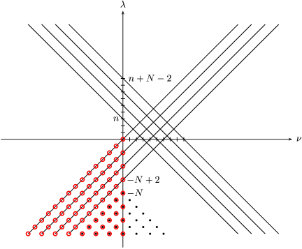
Figure 7.1: ${\mathcal{Z}}_{N}$ ($N=8$) and $L_{\operatorname{even}}$

Hence Proposition 7.3 is proved. ∎

8 Meromorphic continuation of regular symmetry breaking operators ${K}_{{\lambda},{\nu}}^{\mathbb{A}}$

The goal of this chapter is to prove the existence of the meromorphic continuation of our symmetry breaking operator ${\mathbb{A}}_{{\lambda},{\nu}}$, initially holomorphic in an open set $\Omega_{0}$, to $(\lambda,\nu)\in\mathbb{C}^{2}$. Besides, we determine all the poles of the symmetry breaking operator ${\mathbb{A}}_{{\lambda},{\nu}}$ with meromorphic parameter $\lambda$ and $\nu$. The normalized symmetry breaking operators $\widetilde{\mathbb{A}}_{{\lambda},{\nu}}$ depends holomorphically on $(\lambda,\nu)$ in the entire space ${\mathbb{C}}^{2}$. Surprisingly, there exist countably many points in the complex set in ${\mathbb{C}}^{2}$ such that $\widetilde{\mathbb{A}}_{\lambda,\nu}$ vanishes, namely, $\widetilde{\mathbb{A}}_{\lambda,\nu}$ is zero on the set $L_{\operatorname{even}}$ of codimension two in ${\mathbb{C}}^{2}$. We shall prove

Theorem 8.1.

1) $\widetilde{K}_{{\lambda},{\nu}}^{\mathbb{A}}$ is a distribution on $\mathbb{R}^{n}$ that depends holomorphically on parameters $\lambda$ and $\nu$ in the entire plane ${\mathbb{C}}^{2}$.

1. $\widetilde{K}_{{\lambda},{\nu}}^{\mathbb{A}}\in\mathcal{S}ol(\mathbb{R}^{n};\lambda,\nu)$ for all $(\lambda,\nu)\in\mathbb{C}^{2}$, and thus defines a continuous $G^{\prime}$-homomorphism

   $$\widetilde{\mathbb{A}}_{\lambda,\nu}:I(\lambda)\to J(\nu).$$ (8.1)

   This operator $\widetilde{\mathbb{A}}_{\lambda,\nu}$ vanishes if and only if $(\lambda,\nu)\in L_{\operatorname{even}}$, namely,

   $$\lambda,\nu\in-{\mathbb{N}},\,\lambda\equiv\nu\mod 2,\text{ and }\lambda\leq\nu.$$ (8.2)

In what follows, we shall consider the following open subsets in $\mathbb{C}^{2}$:

$$\Omega_{1} :=\{(\lambda,\nu)\in{\mathbb{C}}^{2}:\operatorname{Re}(\lambda-\nu)>0\},$$ (8.3)

$$D_{n-1}^{+} :=\{(\lambda,\nu)\in\mathbb{C}^{2}:\operatorname{Re}(\lambda+\nu)>n-1\},$$

$$D_{n}^{-} :=\{(\lambda,\nu)\in\mathbb{C}^{2}:\operatorname{Re}(\lambda+\nu)<n\}.$$

Obviously, $D_{n-1}^{+}\cup D_{n}^{-}=\mathbb{C}^{2}$. We recall from (7.3)

$$\Omega_{0}=\Omega_{1}\cap D_{n-1}^{+}.$$ (8.4)

The proof of Theorem 8.1 consists of the following two steps:

Step 1. $\Omega_{0}\Rightarrow\Omega_{1}$. Use differential equations, see (8.5) and (8.6).

Step 2. $\Omega_{1}\Rightarrow{\mathbb{C}}^{2}$. Use functional equations, see (8.7) and (8.8).

8.1 Recurrence relations of the distribution kernels ${K}_{{\lambda},{\nu}}^{\mathbb{A}}$

As the first step, we shall use recurrence relations of ${K}_{{\lambda},{\nu}}^{\mathbb{A}}(x,x_{n})$. We set

$$K_{\lambda,\nu}^{\pm}(x,x_{n}):=(x_{n})_{\pm}^{\lambda+\nu-n}(|x|^{2}+x_{n}^{2})^{-\nu}.$$

Then $K_{\lambda,\nu}^{\pm}(x,x_{n})$ is locally integrable if $(\lambda,\nu)\in\Omega_{0}$, and thus gives a distribution on ${\mathbb{R}}^{n}$ with holomorphic parameter $(\lambda,\nu)\in\Omega_{0}$.

Lemma 8.2.

$K_{\lambda,\nu}^{\pm}(x,x_{n})$ extends meromorphically to $\Omega_{1}$ as distributions on ${\mathbb{R}}^{n}$.

Proof.

We only give a proof for $K^{+}(x,x_{n})$; the case for $K(x,x_{n})$ can be shown similarly. First observe that the distribution $K_{\lambda,\nu}^{+}\in\mathcal{D}^{\prime}(\mathbb{R}^{n})$ satisfies the following differential equations when $\operatorname{Re}(\lambda-\nu)\gg 0$ and $\operatorname{Re}(\lambda+\nu)\gg 0$:

$$\frac{\partial}{\partial x_{n}}K_{\lambda+1,\nu}^{+}= (\lambda+\nu-n+1)K_{\lambda,\nu}^{+}-2\nu K_{\lambda,\nu+1}^{+}$$ (8.5)

$$\Delta_{{\mathbb{R}}^{n-1}}K_{\lambda+1,\nu-1}^{+}= 2(\nu-1)(2\nu-n+1)K_{\lambda,\nu}^{+}-4(\nu-1)\nu K_{\lambda+1,\nu+1}^{+}$$ (8.6)

We show the lemma by iterating meromorphic continuations based on the two steps $\Omega\rightsquigarrow\Omega\cup\Omega^{+}$ and $\Omega\rightsquigarrow\Omega\cup\Omega_{+}$ below using (8.5) and (8.6), respectively. Suppose $K_{\lambda,\nu}^{+}$ is proved to extend meromorphically on a certain domain $\Omega$ in $\mathbb{C}^{2}$ as distributions on ${\mathbb{R}}^{n}$. Then the equation (8.5) shows that $K_{\lambda,\nu}^{+}$ extends meromorphically to the following open subset

$$\Omega^{+}:={} \{(\lambda,\nu)\in\mathbb{C}^{2}:(\lambda+1,\nu)\in\Omega\ \text{and}\ (\lambda,\nu+1)\in\Omega\}$$

$$={} (\Omega+(-1,0))\cap(\Omega+(0,-1)).$$

Here we have used the following notation:

$$\Omega+(a,b):=\{(\lambda,\nu)\in{\mathbb{C}}^{2}:(\lambda-a,\nu-b)\in\Omega\}.$$

Likewise, the equation (8.6) shows that $K_{\lambda,\nu}^{+}$ extends meromorphically to

$$\Omega_{+}:=(\Omega+(-1,1))\cap(\Omega+(-1,-1)).$$

Now, first, we set $\Omega=\Omega_{0}$. By iterating the meromorphic continuation process $\Omega\rightsquigarrow\Omega\cup\Omega^{+}$, the distribution $K_{\lambda,\nu}^{+}$ extends meromorphically to the domain $\bigcup_{k=0}^{\infty}(\Omega_{0}+(0,-k))$, which contains

$$\Omega^{\prime}_{0}:=\{(\lambda,\nu)\in{\mathbb{C}}^{2}:\operatorname{Re}(\lambda-\nu)>0,\operatorname{Re}\lambda>\frac{n}{2}\},$$

see Figure 8.1.

Figure 8.1: Analytic continuation from $\Omega_{0}$ to $\Omega_{0}^{\prime}$

Second, we begin with $\Omega^{\prime}_{0}$ and iterate the process $\Omega\rightsquigarrow\Omega\cup\Omega_{+}$. Then we see that $K_{\lambda,\nu}^{+}$ extends meromorphically to the domain $\Omega_{1}=\{(\lambda,\nu)\in{\mathbb{C}}^{2}:\operatorname{Re}(\lambda-\nu)>0\}$, see Figure 8.2.

Figure 8.2: Analytic continuation from $\Omega_{0}^{\prime}$ to $\Omega_{1}$

∎

Lemma 8.3.

If $\operatorname{Re}(\lambda-\nu)>0$, then $\widetilde{K}_{{\lambda},{\nu}}^{\mathbb{A}}\in\mathcal{S}ol(\mathbb{R}^{n};\lambda,\nu)$ and defines a nonzero $G^{\prime}$-intertwining operator $I(\lambda)\to J(\nu)$, to be denoted by the same symbol $\widetilde{\mathbb{A}}_{\lambda,\nu}$. Then $\widetilde{\mathbb{A}}_{\lambda,\nu}$ depends holomorphically on $(\lambda,\nu)$ in the domain $\Omega_{1}$.

Proof.

By Lemma 8.2, ${K}_{{\lambda},{\nu}}^{\mathbb{A}}=K_{\lambda,\nu}^{+}+K_{\lambda,\nu}^{-}$ is a distribution on $\mathbb{R}^{n}$ that depends meromorphically on $\Omega_{1}$. On the other hand, Proposition 7.3 shows that $\widetilde{\mathbb{A}}_{\lambda,\nu}$ is nowhere vanishing and that $\widetilde{\mathbb{A}}_{\lambda,\nu}(\varphi)$ does not have a pole for any $K$-finite vector $\varphi\in I(\lambda)_{K}$ in the domain $\operatorname{Re}(\lambda-\nu)>0$. Now Lemma 8.3 follows from Proposition 3.19. ∎

8.2 Functional equations

Let $\widetilde{\mathbb{T}}_{{m-\nu}}:J(m-\nu)\to J(\nu)$ be the Knapp–Stein intertwining operator for $G^{\prime}$, and $\widetilde{\mathbb{T}}_{{\lambda}}:I(\lambda)\to I(n-\lambda)$ for $G$ with $m=n-1$. The second step of the proof of Theorem 8.1 is to prove the following functional equations (see Theorem 8.5 below):

$$\widetilde{\mathbb{T}}_{{m-\nu}}\circ\widetilde{\mathbb{A}}_{\lambda,m-\nu} =\frac{\pi^{\frac{m}{2}}}{\Gamma(m-\nu)}\widetilde{\mathbb{A}}_{\lambda,\nu}.$$ (8.7)

$$\widetilde{\mathbb{A}}_{n-\lambda,\nu}\circ\widetilde{\mathbb{T}}_{{\lambda}} =\frac{\pi^{\frac{n}{2}}}{\Gamma(n-\lambda)}\widetilde{\mathbb{A}}_{\lambda,\nu}.$$ (8.8)

We begin with

Lemma 8.4.

1) The identity (8.7) holds in the domain $\Omega_{0}=\Omega_{1}\cap D_{n-1}^{+}$ (see (7.3)).

2) The identity (8.8) holds in the domain

$$\Omega_{2}:=\Omega_{1}\cap D_{n}^{-}.$$ (8.9)

Proof.

Since the (renormalized) Knapp–Stein intertwining operator $\widetilde{\mathbb{T}}_{{m-\nu}}$ depends holomorphically on $\nu\in\mathbb{C}$, the composition

$$\widetilde{\mathbb{T}}_{{m-\nu}}\circ\widetilde{\mathbb{A}}_{\lambda,m-\nu}:I(\lambda)\to J(m-\nu)\to J(\nu)$$

is a continuous $G^{\prime}$-homomorphism that depends holomorphically on $(\lambda,\nu)$ by Lemma 8.3 if $\operatorname{Re}(\lambda-(m-\nu))>0$, namely, if $(\lambda,\nu)\in D_{n-1}^{+}$. Thus $\widetilde{\mathbb{A}}_{\lambda,\nu}$ and $\widetilde{\mathbb{T}}_{{m-\nu}}\circ\widetilde{\mathbb{A}}_{\lambda,m-\nu}$ are in $\operatorname{Hom}_{G^{\prime}}(I(\lambda),J(\nu))$ if $(\lambda,\nu)\in\Omega_{0}$.

We recall from Lemma 8.3 that $\widetilde{\mathbb{A}}_{\lambda,\nu}\neq 0$ if $\operatorname{Re}(\lambda-\nu)>0$ and from Proposition 6.8 that $\dim\operatorname{Hom}_{G^{\prime}}(I(\lambda),J(\nu))\leq 1$ if $(\lambda,\nu)\in\Omega_{0}$ ($\subset\mathbb{C}^{2}-/\!/$). Therefore there exists $b(\lambda,\nu)\in\mathbb{C}$ such that

$$\widetilde{\mathbb{T}}_{{m-\nu}}\circ\widetilde{\mathbb{A}}_{\lambda,m-\nu}=b(\lambda,\nu)\widetilde{\mathbb{A}}_{\lambda,\nu}$$

for $(\lambda,\nu)\in\Omega_{0}$. Applying these operators to the trivial one-dimensional $K$-type $\mathbf{1}_{\lambda}\in I(\lambda)_{K}$, we get from Proposition 7.4 and Proposition 4.6

$$\frac{\pi^{\frac{m}{2}}}{\Gamma(m-\nu)}\frac{\pi^{\frac{m}{2}}}{2^{\lambda-1}\Gamma(\lambda)}\mathbf{1}_{\nu}=b(\lambda,\nu)\frac{\pi^{\frac{m}{2}}}{2^{\lambda-1}\Gamma(\lambda)}\mathbf{1}_{\nu},$$

and therefore $b(\lambda,\nu)=\frac{\pi^{\frac{m}{2}}}{\Gamma(m-\nu)}$. Thus we have proved (8.7) in the domain $\Omega_{0}=\Omega_{1}\cap D_{n-1}^{+}$.

Similarly the composition

$$\widetilde{\mathbb{A}}_{n-\lambda,\nu}\circ\widetilde{\mathbb{T}}_{{\lambda}}:I(\lambda)\to I(n-\lambda)\to J(\nu)$$

is a continuous $G^{\prime}$-homomorphism if $\operatorname{Re}((n-\lambda)-\nu)>0$, namely, if $(\lambda,\nu)\in D_{n}^{-}$. Therefore there exists $c(\lambda,\nu)\in\mathbb{C}$ such that

$$\widetilde{\mathbb{A}}_{n-\lambda,\nu}\circ\widetilde{\mathbb{T}}_{{\lambda}}=c(\lambda,\nu)\widetilde{\mathbb{A}}_{\lambda,\nu}$$

if $\operatorname{Re}(\lambda-\nu)>0$ and $\operatorname{Re}(\lambda+\nu)<n$. Applying these operators to $\mathbf{1}_{\lambda}$, we get

$$\frac{\pi^{\frac{n-1}{2}}}{\Gamma(n-\lambda)}\frac{\pi^{\frac{n}{2}}}{\Gamma(\lambda)}\mathbf{1}_{\nu}=c(\lambda,\nu)\frac{\pi^{\frac{n-1}{2}}}{\Gamma(\lambda)}\mathbf{1}_{\nu},$$

whence $c(\lambda,\nu)=\frac{\pi^{\frac{n}{2}}}{\Gamma(n-\lambda)}$. Thus we have proved (8.8) in the domain $\Omega_{2}=\Omega_{1}\cap D_{n}^{-}$. ∎

Now we are ready to complete the proof of Theorem 8.1.

Proof of Theorem 8.1.

In order to extend ${K}_{{\lambda},{\nu}}^{\mathbb{A}}$ meromorphically, it is sufficient to prove it for ${K}_{{\lambda},{\nu}}^{\mathbb{A}}|_{{\mathbb{R}}^{n}}$ by Proposition 3.18. Then it follows from Lemma 8.2 that ${K}_{{\lambda},{\nu}}^{\mathbb{A}}$ extends meromorphically from $\Omega_{0}$ to $\Omega_{1}$ as distributions on ${\mathbb{R}}^{n}$. In turn, ${K}_{{\lambda},{\nu}}^{\mathbb{A}}$ extends meromorphically to the domain $\Omega_{1}\cup D_{n-1}^{+}$ as a distribution on $\mathbb{R}^{n}$ by Lemma 8.4 (1), and it extends meromorphically to the domain $\Omega_{1}\cup D_{n}^{-}$ as a distribution on $\mathbb{R}^{n}$ by Lemma 8.4 (2). Hence ${K}_{{\lambda},{\nu}}^{\mathbb{A}}$ extends meromorphically to ${\mathbb{C}}^{2}$. ∎

Now, by Theorem 8.1, Lemma 8.4 can be strengthened as follows:

Theorem 8.5.

The functional equations (8.7) and (8.8) hold for entire $(\lambda,\nu)\in{\mathbb{C}}^{2}$, namely,

$$\widetilde{\mathbb{T}}_{{m-\nu}}\circ\widetilde{\mathbb{A}}_{\lambda,m-\nu} =\frac{\pi^{\frac{m}{2}}}{\Gamma(m-\nu)}\widetilde{\mathbb{A}}_{\lambda,\nu}\qquad \text{for $(\lambda,\nu)\in{\mathbb{C}}^{2}$},$$ (8.10)

$$\widetilde{\mathbb{A}}_{n-\lambda,\nu}\circ\widetilde{\mathbb{T}}_{{\lambda}} =\frac{\pi^{\frac{n}{2}}}{\Gamma(n-\lambda)}\widetilde{\mathbb{A}}_{\lambda,\nu}\qquad \text{for $(\lambda,\nu)\in{\mathbb{C}}^{2}$}.$$ (8.11)

8.3 Support of $\widetilde{K}_{{\lambda},{\nu}}^{\mathbb{A}}$

We determine the support of the distribution kernel $\widetilde{K}_{{\lambda},{\nu}}^{\mathbb{A}}$ when it is nonzero, equivalently, by Theorem 8.1 (2), namely, when $(\lambda,\nu)\notin L_{\operatorname{even}}$.

Proposition 8.6.

Suppose $(\lambda,\nu)\notin L_{\operatorname{even}}$, equivalently, $\widetilde{\mathbb{A}}_{\lambda,\nu}\neq 0$. Then

$$\operatorname{Supp}\widetilde{K}_{{\lambda},{\nu}}^{\mathbb{A}}=\begin{cases}S^{n-1}&\text{if\/ $(\lambda,\nu)\in\backslash\!\backslash-\mathbb{X}$},\\ \{[p_{+}]\}&\text{if\/ $(\lambda,\nu)\in/\!/-L_{\operatorname{even}}$},\\ G/P&\text{otherwise}.\end{cases}$$

Proof.

We recall from (7.2) that as a distribution on $\mathbb{R}^{n}-\{0\}$,

$${K}_{{\lambda},{\nu}}^{\mathbb{A}}(x,x_{n})|_{{\mathbb{R}}^{n}-\{0\}}=r^{\lambda-\nu-1}|\omega_{n}|^{\lambda+\nu-n}$$

in the polar coordinates $(x,x_{n})=r\omega$. Since the function

$$\omega_{n}:S^{n-1}\to{\mathbb{R}},\quad\omega=(\omega_{1},\cdots,\omega_{n})\mapsto\omega_{n}$$

is regular at $\omega_{n}=0$, the distribution $|\omega_{n}|^{\lambda+\nu-n}$ on $S^{n-1}$ has a simple pole at $\lambda+\nu=n-1,n-3,\dotsc$, and the support of its residue is equal to $S^{n-1}=\{\omega_{n}=0\}$. In light of Remark 7.2, we have thus

$$\operatorname{Supp}(\widetilde{K}_{{\lambda},{\nu}}^{\mathbb{A}}|_{\mathbb{R}^{n}-\{0\}})=\mathbb{R}^{n-1}-\{0\} \text{ if }(\lambda,\nu)\in\backslash\!\backslash-\mathbb{X},$$

$$\operatorname{Supp}(\widetilde{K}_{{\lambda},{\nu}}^{\mathbb{A}}|_{\mathbb{R}^{n}-\{0\}})=\emptyset \text{ if }(\lambda,\nu)\in/\!/-\mathbb{X}.$$

For $(\lambda,\nu)\in\mathbb{X}$, $\Gamma(\frac{\lambda+\nu-n+1}{2})\Gamma(\frac{\lambda-\nu}{2})$ has a pole of order two, and therefore $\widetilde{K}_{{\lambda},{\nu}}^{\mathbb{A}}|_{\mathbb{R}^{n}-\{0\}}=0$. Hence

$$\operatorname{Supp}(\widetilde{K}_{{\lambda},{\nu}}^{\mathbb{A}}|_{{\mathbb{R}}^{n}-\{0\}})=\emptyset\quad\text{if }(\lambda,\nu)\in{\mathbb{X}}.$$

Now we get Proposition 8.6 by Lemma 6.1. ∎

8.4 Renormalization $\tilde{\tilde{\mathbb{A}}}_{\lambda,\nu}$ for $\nu\in-\mathbb{N}$

We have seen in Theorem 8.1 (2) that the distribution $\widetilde{\mathbb{A}}_{\lambda,\nu}$ with holomorphic parameter $(\lambda,\nu)$ vanishes in the discrete subset of $\mathbb{C}^{2}$, i.e., if $(\lambda,\nu)\in L_{\operatorname{even}}$. In this section we renormalize $\widetilde{\mathbb{A}}_{\lambda,\nu}$ as a function of a single variable $\lambda$ by fixing $\nu\in-\mathbb{N}$ in order to obtain nonzero symmetry breaking operators.

Suppose $\nu\in-{\mathbb{N}}$. Then the factor $(\xi_{n+1}-\xi_{0})^{-\nu}$ of the distribution kernel ${k}_{{\lambda},{\nu}}^{\mathbb{A}}(\xi)$ in (7.4) is a polynomial, and thus the distribution kernel ${k}_{{\lambda},{\nu}}^{\mathbb{A}}$ has a better regularity.

Proposition 8.7.

Suppose $\nu\in-\mathbb{N}$. Then

$$\tilde{\tilde{K}}^{\mathbb{A}}_{{\lambda},{\nu}}(x,x_{n}):=\frac{1}{\Gamma(\frac{\lambda+\nu-n+1}{2})}{K}_{{\lambda},{\nu}}^{\mathbb{A}}(x,x_{n})=\Gamma(\frac{\lambda-\nu}{2})\widetilde{K}_{{\lambda},{\nu}}^{\mathbb{A}}(x,x_{n})$$ (8.12)

extends to a distribution on $K/M\simeq G/P$ which depends holomorphically in $\lambda$ in the whole complex plane. Then there exists a nonzero $G^{\prime}$-intertwining operator

$$\tilde{\tilde{\mathbb{A}}}_{\lambda,\nu}:I(\lambda)\to J(\nu),$$ (8.13)

whose distribution kernel is $\tilde{\tilde{K}}^{\mathbb{A}}_{{\lambda},{\nu}}$. Further,

$$\tilde{\tilde{\mathbb{A}}}_{\lambda,\nu}(\mathbf{1}_{\lambda})=\frac{\pi^{\frac{n-1}{2}}\Gamma(\frac{\lambda-\nu}{2})}{\Gamma(\lambda)}\mathbf{1}_{\nu}.$$ (8.14)

Remark 8.8.

For a fixed $\nu\in-\mathbb{N}$, $(\lambda,\nu)\in L_{\operatorname{even}}$ if and only if $\lambda$ is a (simple) pole of $\Gamma(\frac{\lambda-\nu}{2})$. In this case, the formula (8.14) amounts to

$$\tilde{\tilde{\mathbb{A}}}_{\lambda,\nu}(\mathbf{1}_{\lambda})=\frac{\pi^{\frac{n-1}{2}}(-\lambda)!(-1)^{\lambda+l}}{l!}\mathbf{1}_{\nu},$$

where $l\in\mathbb{N}$ is defined by the relation $\nu-\lambda=2l$.

Proof of Proposition 8.7.

In the coordinates $\eta=(\eta_{0},\dots,\eta_{n})\in S^{n}$,

$$\frac{1}{\Gamma(\frac{\lambda+\nu-n+1}{2})}|\eta_{n}|^{\lambda+\nu-n}$$

is a nonzero distribution on $S^{n}$ which is holomorphic in $\lambda$ in the whole complex plane because $\eta_{n}:S^{n}\to{\mathbb{R}}$ is regular at $\eta_{n}=0$. On the other hand, since $\nu\in-\mathbb{N}$, $(1-\eta_{0})^{-\nu}$ is a polynomial in $\eta_{0}$,

$$\frac{1}{\Gamma(\frac{\lambda+\nu-n+1}{2})}|\eta_{n}|^{\lambda+\nu-n}(1-\eta_{0})^{-\nu}$$

is well-defined and gives a distribution on $S^{n}\simeq G/P$ with holomorphic parameter $\lambda\in\mathbb{C}$. Moreover it is nonzero for any $\lambda$ in any neighbourhood of $\eta$ with $\eta_{0}\neq 1$ and $\eta_{n}=0$. Now Proposition 8.7 follows from (7.6). ∎

The following proposition shows that the renormalized symmetry breaking operator $\tilde{\tilde{\mathbb{A}}}_{\lambda,\nu}$ is generically regular in the sense of Definition 3.3.

Proposition 8.9 (Support of $\tilde{\tilde{K}}^{\mathbb{A}}_{{\lambda},{\nu}}$).

Suppose $\nu\in-\mathbb{N}$. Then the distribution kernel $\tilde{\tilde{K}}^{\mathbb{A}}_{{\lambda},{\nu}}$ of the symmetry breaking operator $\tilde{\tilde{\mathbb{A}}}_{\lambda,\nu}$ has the following support:

$$\operatorname{Supp}\tilde{\tilde{K}}^{\mathbb{A}}_{{\lambda},{\nu}}=\begin{cases}G/P&\text{if\/ $(\lambda,\nu)\notin\backslash\!\backslash$},\\ S^{n-1}&\text{if\/ $(\lambda,\nu)\in\backslash\!\backslash$}.\end{cases}$$

Proof.

As a distribution on $G/P$, we have

$$\operatorname{Supp}\frac{1}{\Gamma(\frac{\lambda+\nu-n+1}{2})}|\eta_{n}|^{\lambda+\nu-n}=\begin{cases}G/P&\text{if\/ $(\lambda,\nu)\notin\backslash\!\backslash$},\\ S^{n-1}&\text{if\/ $(\lambda,\nu)\in\backslash\!\backslash$}.\end{cases}$$

The multiplication of $(1-\eta_{0})^{-\nu}\in C^{\infty}(S^{n})$ is well-defined, and does not affect the support because the equation $1-\eta_{0}=0$ holds only if $\eta=(1,0,\dots,0)\in S^{n}$. Thus we proved the Proposition. ∎

9 Singular symmetry breaking operator $\widetilde{\mathbb{B}}_{\lambda,\nu}$

We have seen in Lemma 6.7 that singular symmetry breaking operators exist only if $(\lambda,\nu)\in\backslash\!\backslash$. In this chapter we construct a family of singular symmetry breaking operators

$$\widetilde{\mathbb{B}}_{\lambda,\nu}:I(\lambda)\to J(\nu)\quad\text{for}\quad(\lambda,\nu)\in\backslash\!\backslash$$ (9.1)

by giving an explicit formula of the distribution kernel, see (9.6). The operator $\widetilde{\mathbb{B}}_{{\lambda},{\nu}}$ depends holomorphically on $\lambda\in{\mathbb{C}}$ (or on $\nu\in{\mathbb{C}}$) under the constraints that $(\lambda,\nu)\in\backslash\!\backslash$. We find a necessary and sufficient condition that $\widetilde{\mathbb{B}}_{{\lambda},{\nu}}\neq 0$. Other singular symmetry breaking operators are only the differential operators $\widetilde{\mathbb{C}}_{{\lambda},{\nu}}$ that will be discussed in the next chapter.

The classification of singular symmetry breaking operators will be given in Proposition 11.14.

9.1 Singular symmetry breaking operator $\widetilde{\mathbb{B}}_{\lambda,\nu}$

For $(\lambda,\nu)\in\backslash\!\backslash$, we define $k\in\mathbb{N}$ by the relation

$$\lambda+\nu=n-1-2k.$$ (9.2)

In what follows, we shall fix $k\in\mathbb{N}$ and discuss the meromorphic continuation by varying $\nu\in\mathbb{C}$ (or $\lambda\in\mathbb{C}$) under the constraints (9.2).

For $\xi=(\xi_{0},\dots,\xi_{n+1})\in\Xi$, we set

$$k_{\lambda,\nu}^{\mathbb{B}}(\xi):=2^{2k+1+\nu}\delta^{(2k)}(\xi_{n})(\xi_{n+1}-\xi_{0})^{-\nu}.$$

Then $k_{\lambda,\nu}^{\mathbb{B}}(\xi)$ is a distribution on $\Xi$, when $\operatorname{Re}\nu\ll 0$. Further $k_{\lambda,\nu}^{\mathbb{B}}(\xi)\in\mathcal{D}^{\prime}_{\lambda-n}(\Xi)\simeq I(n-\lambda)^{-\infty}$ and, as in (7.7), it satisfies a $P^{\prime}$-covariance

$$k_{\lambda,\nu}^{\mathbb{B}}(me^{-tH}n\xi)=e^{\nu t}k_{\lambda,\nu}^{\mathbb{B}}(\xi)$$ (9.3)

for any $me^{-tH}n\in M^{\prime}AN_{+}^{\prime}=P^{\prime}$. By (9.10) we have:

$$\iota_{N}^{*}k_{\lambda,\nu}^{\mathbb{B}} =(|x|^{2}+x_{n}^{2})^{-\nu}\delta^{(2k)}(x_{n}).$$ (9.4)

$$(\iota_{K}^{*}k_{\lambda,\nu}^{\mathbb{B}})(\eta) =2^{2k+1+\nu}\delta^{(2k)}(\eta_{n})(1-\eta_{0})^{-\nu}.$$ (9.5)

In order to give the meromorphic continuation of the distribution kernel, which is initially holomorphic when $\operatorname{Re}\nu\ll 0$, we normalize (9.4) as

$$\widetilde{K}_{{\lambda},{\nu}}^{\mathbb{B}}(x,x_{n}):={} \frac{1}{\Gamma(\frac{\lambda-\nu}{2})}(|x|^{2}+x_{n}^{2})^{-\nu}\delta^{(2k)}(x_{n})$$ (9.6)

$$={} \frac{1}{\Gamma(\frac{n-1}{2}-\nu-k)}(|x|^{2}+x_{n}^{2})^{-\nu}\delta^{(2k)}(x_{n}).$$

The main properties of $\widetilde{\mathbb{B}}_{{\lambda},{\nu}}$ are summarized as follows.

Theorem 9.1.

Suppose $(\lambda,\nu)\in\backslash\!\backslash$.

1. For $(\lambda,\nu)\in\backslash\!\backslash$ with $\operatorname{Re}(\lambda-\nu)>0$, $\widetilde{K}_{{\lambda},{\nu}}^{\mathbb{B}}$ is well-defined as a distribution on $\mathbb{R}^{n}$, and satisfies:

   $$\widetilde{K}_{{\lambda},{\nu}}^{\mathbb{B}}(x,x_{n})=\frac{1}{\Gamma(\frac{n-1}{2}-\nu-k)}\sum_{i=0}^{k}\frac{(-1)^{i}(2k)!(\nu)_{i}}{(2k-2i)!\,i!}\,|x|^{-2\nu-2i}\delta^{(2k-2i)}(x_{n}).$$ (9.7)

2. Fix $k\in\mathbb{N}$. Then $\widetilde{K}_{{\lambda},{\nu}}^{\mathbb{B}}$ extends to a distribution on $\mathbb{R}^{n}$ that depends holomorphically on $\nu$ in the entire plane $\mathbb{C}$ (or $\lambda\in\mathbb{C}$).

3. $\widetilde{K}_{{\lambda},{\nu}}^{\mathbb{B}}\in\mathcal{S}ol(\mathbb{R}^{n};\lambda,\nu)$ (see (6.8) for the definition) for all $(\lambda,\nu)\in\backslash\!\backslash$, and induces a continuous $G^{\prime}$-intertwining operator

   $$\widetilde{\mathbb{B}}_{\lambda,\nu}:I(\lambda)\to J(\nu).$$

4. $\widetilde{\mathbb{B}}_{\lambda,\nu}=0$ if and only if $n$ is odd and $(\lambda,\nu)\in L_{\operatorname{even}}$.

For the proof of Theorem 9.1, we use:

Lemma 9.2.

1. For ${\operatorname{Re}}\nu\ll 0$,

   $$\Bigl{(}\frac{\partial}{\partial x_{n}}\Bigr{)}^{i}(|x|^{2}+x_{n}^{2})^{-\nu}\Bigm{|}_{x_{n}=0}=\begin{cases}0&\text{if\/ $i=2j+1$},\\ \frac{(-1)^{j}(2j)!\,\Gamma(\nu+j)}{j!\,\Gamma(\nu)}|x|^{-2\nu-2j}&\text{if\/ $i=2j$}.\end{cases}$$

2. Suppose $\operatorname{Re}\nu<\frac{n-1}{2}-N$. Then $|x|^{-2\nu-2j}\in L_{\operatorname{loc}}^{1}(\mathbb{R}^{n-1})$ for all $0\leq j\leq[\frac{N}{2}]$, and we have the following identity of distributions on $\mathbb{R}^{n}$:

   $$(|x|^{2}+x_{n}^{2})^{-\nu}\delta^{(N)}(x_{n})=\sum_{j=0}^{[\frac{N}{2}]}\frac{(-1)^{j}N!\,\Gamma(\nu+j)}{(N-2j)!\,j!\,\Gamma(\nu)}|x|^{-2\nu-2j}\delta^{(N-2j)}(x_{n}).$$

Proof.

1) The expansion

$$(A+y^{2})^{\mu}=\sum_{i=0}^{\infty}\frac{\Gamma(\mu+1)}{i!\,\Gamma(\mu+1-i)}A^{\mu-i}y^{2i}$$

implies

$$\Bigl{(}\frac{\partial}{\partial y}\Bigr{)}^{2i}(A+y^{2})^{\mu}\Bigm{|}_{y=0}=\frac{(2i)!\,\Gamma(\mu+1)}{i!\,\Gamma(\mu+1-i)}A^{\mu-i}.$$ (9.8)

Now the statement is clear.

2) For a test function $\varphi\in C_{0}^{\infty}(\mathbb{R}^{n})$,

$$\Bigl{(}\frac{\partial}{\partial x_{n}}\Bigr{)}^{N}\bigm{|}_{x_{n}=0}((|x|^{2}+x_{n}^{2})^{-\nu}\varphi(x,x_{n}))$$

$$=\sum_{i=0}^{N}\begin{pmatrix}N\\ i\end{pmatrix}\left(\Bigl{(}\frac{\partial}{\partial x_{n}}\Bigr{)}^{i}(|x|^{2}+x_{n}^{2})^{-\nu}\right)\left(\Bigl{(}\frac{\partial}{\partial x_{n}}\Bigr{)}^{N-i}\varphi(x,x_{n})\right)\biggm{|}_{x_{n}=0}.$$

Substituting the formula of (1) into the right-hand side, we get (2). ∎

9.2 $K$-finite vectors and singular operators $\widetilde{\mathbb{B}}_{{\lambda},{\nu}}$

Proposition 9.3.

Suppose $(\lambda,\nu)\in\backslash\!\backslash$. We define $k\in\mathbb{N}$ by the relation (9.2). Then $\langle\widetilde{K}_{{\lambda},{\nu}}^{\mathbb{B}},F\rangle=(-1)^{k}2^{k}(2k-1)!!\langle\widetilde{K}_{{\lambda},{\nu}}^{\mathbb{A}},F\rangle$ for any $F\in I(\lambda)_{K}$.

We give a proof of Proposition 9.3 in parallel to the argument of Chapter 7. A new ingredient is the following:

Lemma 9.4.

Suppose $(\lambda,\nu)\in\backslash\!\backslash$.

1. If $N$ is odd or $\psi\perp{\mathcal{H}}^{N}(S^{n-1})^{O(n-1)}$, then

   $$\int_{S^{n-1}}\psi(\omega)\delta^{(2k)}(\omega_{n})=0.$$

2. If $N$ is even, then

   $$\int_{S^{n-1}}\widetilde{C}_{N}^{\frac{n}{2}-1}(\omega_{n})\delta^{(2k)}(\omega_{n})=(-1)^{k}2^{k}(2k-1)!!\frac{d_{n,N}(\lambda,\nu)g(\lambda,\nu)}{\Gamma(\frac{\lambda+\nu-n+1}{2})}.$$

Proof.

In light of the residue formula

$$\frac{1}{\Gamma(\frac{\mu+1}{2})}|t|^{\mu}\Bigm{|}_{\mu=-1-2k}=\frac{(-1)^{k}}{2^{k}(2k-1)!!}\delta^{(2k)}(t)\quad\text{in $\mathcal{D}^{\prime}(\mathbb{R})$},$$

the statements follow from Lemma 7.6. ∎

Owing to Lemma 9.4, the following lemma is derived as in Lemma 7.7.

Lemma 9.5.

Let $(\lambda,\nu)\in\backslash\!\backslash$. Let $k\in{\mathbb{N}}$ be as in (9.2).

1. Suppose $N\in\mathbb{N}$, $\psi\in{\mathcal{H}}^{N}(S^{n-1})$, and $h\in\mathbb{C}[s]$. Then we have:

   $$\langle\widetilde{K}_{{\lambda},{\nu}}^{\mathbb{B}},F_{\lambda}[\psi,h]\rangle=0\quad\text{if $N$ is odd or }\psi\perp{\mathcal{H}}^{N}(S^{n-1}).$$

2. If $N\in 2{\mathbb{N}}$, then

   $$\langle\widetilde{K}_{{\lambda},{\nu}}^{\mathbb{B}},F_{\lambda}[\widetilde{C}_{N}^{\frac{n}{2}-1}(\omega_{n}),h]\rangle=cP_{\frac{\lambda-\nu+N}{2},\frac{\lambda+\nu+N}{2}}(h)\prod_{j=0}^{\frac{N}{2}-1}\Bigl{(}\frac{\lambda-\nu}{2}+j\Bigr{)}\Bigl{(}\frac{\lambda+\nu-n}{2}-j\Bigr{)},$$

   where the non-zero constant $c$ is given by

   $$(-1)^{k}2^{k}(2k-1)!!\frac{2^{3-\lambda-n}\pi^{\frac{n}{2}}\Gamma(n+N-1)}{\Gamma(\frac{n-1}{2})\Gamma(N+1)}.$$

Proof of Proposition 9.3.

Clear from the comparison of Lemma 7.7 and Lemma 9.5. ∎

As a special case of Proposition 9.3, we obtain

Proposition 9.6.

For $(\lambda,\nu)\in\backslash\!\backslash$, we set $k\in\mathbb{N}$ by $\lambda+\nu=n-1-2k$. Then we have

$$\widetilde{\mathbb{B}}_{\lambda,\nu}(\mathbf{1}_{\lambda})=\frac{(-1)^{k}2^{k}\pi^{\frac{n-1}{2}}(2k-1)!!}{\Gamma(\lambda)}\mathbf{1}_{\nu}.$$ (9.9)

Proof.

We recall from Proposition 7.4 that

$$\widetilde{\mathbb{A}}_{{\lambda},{\nu}}({\bf{1}}_{\lambda})=\frac{\pi^{\frac{n-1}{2}}}{\Gamma(\lambda)}{\bf{1}}_{\nu}.$$

Now the statement is immediate from Proposition 9.3. ∎

As another consequence of Proposition 9.3, we have

Proposition 9.7.

$\langle\widetilde{K}_{{\lambda},{\nu}}^{\mathbb{B}},F\rangle=0$ for any $F\in I(\lambda)_{K}$ if and only if $(\lambda,\nu)\in L_{\operatorname{even}}$.

Proof.

The proof is the same as that of Proposition 7.3. ∎

9.3 Proof of Theorem 9.1

Proof of Theorem 9.1.

1) Let $k$ be defined as in (9.2). Then $|x|^{-2\nu-2i}\in L^{1}_{\operatorname{loc}}(\mathbb{R}^{n-1})$ for all $0\leq i\leq k$ if and only if $\operatorname{Re}(\lambda-\nu)>0$. By Lemma 9.2 we get the expansion formula (9.7), which shows that $\widetilde{K}_{{n-1-2k-\nu},{\nu}}^{\mathbb{B}}$ extends to a distribution on $\mathbb{R}^{n}$ depending holomorphically on $\nu$ in the domain $\{\nu\in\mathbb{C}:\operatorname{Re}\nu<\frac{n-1}{2}-k\}$.

2) By the expression (9.7), the assertion is clear.

3) It is easy to see $\widetilde{K}_{{\lambda},{\nu}}^{\mathbb{B}}\in\mathcal{S}ol(\mathbb{R}^{n};\lambda,\nu)$ for $\operatorname{Re}\nu\ll 0$. Since $\widetilde{K}_{{\lambda},{\nu}}^{\mathbb{B}}$ extends holomorphically to $(\lambda,\nu)\in\backslash\!\backslash$ as a distribution on $\mathbb{R}^{n}$, the third statement follows from Proposition 3.18.

4)  Clear from Proposition 9.7. ∎

9.4 Support of the distribution kernel of $\widetilde{\mathbb{B}}_{\lambda,\nu}$

We have seen in Theorem 9.1 that $\widetilde{\mathbb{B}}_{\lambda,\nu}\neq 0$ if and only if $(\lambda,\nu)\in\backslash\!\backslash-L_{\operatorname{even}}$. In this section, we find the support of the distribution kernel of $\widetilde{K}_{{\lambda},{\nu}}^{\mathbb{B}}$.

Proposition 9.8.

Assume

$$(\lambda,\nu)\in\backslash\!\backslash-L_{\operatorname{even}}=\begin{cases}\backslash\!\backslash-L_{\operatorname{even}}\quad&\text{($n:odd$),}\\ \backslash\!\backslash&\text{($n:even$).}\end{cases}$$

Then the kernel of the non-zero singular symmetry breaking operator $\widetilde{\mathbb{B}}_{\lambda,\nu}$ has the following support:

$$\operatorname{Supp}\widetilde{K}_{{\lambda},{\nu}}^{\mathbb{B}}=\begin{cases}\{[p_{+}]\}&\text{if\/ $(\lambda,\nu)\in{\mathbb{X}}-L_{\operatorname{even}}$},\\ S^{n-1}&\text{if\/ $(\lambda,\nu)\in\backslash\!\backslash-{\mathbb{X}}$}.\end{cases}$$

Proof.

Suppose $(\lambda,\nu)\in\backslash\!\backslash-L_{\operatorname{even}}$. By Lemma 6.1 and the definition (9.6) of $\widetilde{K}_{{\lambda},{\nu}}^{\mathbb{B}}$, $\operatorname{Supp}\widetilde{K}_{{\lambda},{\nu}}^{\mathbb{B}}$ is either $\{[p_{+}]\}$ or $S^{n-1}$. Since $|x|^{2}+x_{n}^{2}$ is non-zero on ${\mathbb{R}}^{n}-\{0\}$, $(|x|^{2}+x_{n}^{2})^{-\nu}$ is a nowhere vanishing smooth function on ${\mathbb{R}}^{n}-\{0\}$. Therefore, the restriction of $\widetilde{K}_{{\lambda},{\nu}}^{\mathbb{B}}$ to the open set ${\mathbb{R}}^{n}-\{0\}$ vanishes if and only if $\Gamma(\frac{\lambda-\nu}{2})=\infty$, namely, $(\lambda,\nu)\in/\!/$. Thus Proposition is proved. ∎

9.5 Renormalization $\tilde{\tilde{\mathbb{B}}}_{\lambda,\nu}$ for $(\lambda,\nu)\in L_{\operatorname{even}}$ with $n$ odd

For $n$ odd, the singular symmetry breaking operator $\widetilde{\mathbb{B}}_{\lambda,\nu}$ vanishes when $(\lambda,\nu)\in L_{\operatorname{even}}$, see Theorem 9.1. As we renormalized the (generically) regular symmetry breaking operator $\widetilde{\mathbb{A}}_{\lambda,\nu}$ for $\nu\in-\mathbb{N}$ in Section 8.4, we will renormalize $\widetilde{\mathbb{B}}_{\lambda,\nu}$ for $\nu\in-\mathbb{N}$ as follows. For $(\lambda,\nu)\in L_{\operatorname{even}}$ with $n$ odd, we define $k\in\mathbb{N}$ by $\lambda+\nu=n-1-2k$ and set

$$\tilde{\tilde{K}}_{{\lambda},{\nu}}^{\mathbb{B}}(x,x_{n}):={} (|x|^{2}+x_{n}^{2})^{-\nu}\delta^{(2k)}(x_{n})$$

$$={} \sum_{i=0}^{k}\frac{(-1)^{i}(2k)!(\nu)_{i}}{(2k-2i)!\,i!}\,|x|^{-2\nu-2i}\delta^{(2k-2i)}(x_{n}),$$ (9.10)

see (9.7) for $\widetilde{K}_{{\lambda},{\nu}}^{\mathbb{B}}$. Then $\tilde{\tilde{K}}_{{\lambda},{\nu}}^{\mathbb{B}}\in\mathcal{S}ol(\mathbb{R}^{n};\lambda,\nu)$ and we have a $G^{\prime}$-intertwining operator

$$\tilde{\tilde{\mathbb{B}}}_{{\lambda},{\nu}}:I(\lambda)\to J(\lambda)$$ (9.11)

with $\tilde{\tilde{K}}_{{\lambda},{\nu}}^{\mathbb{B}}$ its distribution kernel. Since $L_{\operatorname{even}}$ is a discrete set in ${\mathbb{C}}^{2}$, there is no continuous parameter for $\tilde{\tilde{\mathbb{B}}}_{{\lambda},{\nu}}$. We note that $L_{\operatorname{even}}\subset\mathbb{X}$ for $n$ odd. We shall prove in Theorem 12.2 (4) that $\tilde{\tilde{\mathbb{B}}}_{\lambda,\nu}$ is a scalar multiple of $\tilde{\tilde{\mathbb{A}}}_{\lambda,\nu}$ for any $(\lambda,\nu)\in L_{\operatorname{even}}$ if $n$ is odd. The following proposition is clear from (9.10).

Proposition 9.9.

Suppose $n$ is odd and $(\lambda,\nu)\in L_{\operatorname{even}}$. Then $\tilde{\tilde{\mathbb{B}}}_{\lambda,\nu}\neq 0$ and

$$\operatorname{Supp}\tilde{\tilde{K}}_{{\lambda},{\nu}}^{\mathbb{B}}=S^{n-1}.$$

10 Differential symmetry breaking operators

In this chapter we give a brief review on differential symmetry breaking operators. Nontrivial such operators from $I(\lambda)$ to $J(\nu)$ exist if and only if $\nu-\lambda\in/\!/$, and explicit formulae of all such operators were recently found in [13, 24]. The new ingredient is Proposition 10.7, which gives an explicit action of the normalized differential symmetry breaking operators $\widetilde{\mathbb{C}}_{\lambda,\nu}$ on the spherical vectors. In Chapter 12, we shall see that these differential symmetry breaking operators arise as the residues of the (generically) regular symmetry breaking operators ${\mathbb{A}}_{\lambda,\nu}$ except for the discrete set $L_{\operatorname{even}}$ (Theorem 12.2).

10.1 Power of the Laplacian

We begin with the classical results on conformally covariant differential operators acting on line bundles on the sphere (“$G=G^{\prime}=O(n+1,1)$ case” in the general setting of Chapter 3).

Let ${\mathfrak{g}}_{\mathbb{C}}$ be the complexified Lie algebra of ${\mathfrak{g}}={\mathfrak{o}}(n+1,1)$, and ${\mathfrak{p}}_{\mathbb{C}}={\mathfrak{m}}_{\mathbb{C}}+{\mathfrak{a}}_{\mathbb{C}}+({\mathfrak{n}}_{+})_{\mathbb{C}}$ the complexification of the Levi decomposition of the minimal parabolic subalgebra ${\mathfrak{p}}={\mathfrak{m}}+{\mathfrak{a}}+{\mathfrak{n}}_{+}$ (see (2.9)). We note that ${\mathfrak{p}}_{\mathbb{C}}$ is a maximal parabolic subalgebra of ${\mathfrak{g}}_{\mathbb{C}}\simeq{\mathfrak{o}}(n+2,{\mathbb{C}})$. Let $H$ be the generator of ${\mathfrak{a}}$ defined in (2.4) and denote by ${\mathbb{C}}_{\lambda}$ the ${\mathfrak{p}_{\mathbb{C}}}$-module given by

$${\mathfrak{p}_{\mathbb{C}}}\to{\mathfrak{p}_{\mathbb{C}}}/({\mathfrak{m}}_{\mathbb{C}}+{\mathfrak{n}}_{\mathbb{C}}^{+})\simeq{\mathfrak{a}}_{\mathbb{C}}={\mathbb{C}}H\to{\mathbb{C}},\quad tH\mapsto t\lambda.$$

We define a generalized Verma module by

$$\operatorname{ind}_{{\mathfrak{p}_{\mathbb{C}}}}^{{\mathfrak{g}_{\mathbb{C}}}}(\lambda)\equiv\operatorname{ind}_{{\mathfrak{p}_{\mathbb{C}}}}^{{\mathfrak{g}_{\mathbb{C}}}}({\mathbb{C}}_{\lambda}):=U({\mathfrak{g}_{\mathbb{C}}})\otimes_{U({\mathfrak{p}_{\mathbb{C}}})}{\mathbb{C}}_{\lambda}.$$

Then the following result holds (e.g. [2, 5]):

Lemma 10.1.

Let $n\geq 2$. Let $G=O(n+1,1)$ with $n\geq 2$. Then the following three conditions on $(\lambda,\nu)\in{\mathbb{C}}^{2}$ are equivalent:

1. $\operatorname{Hom}_{\mathfrak{g}}(\operatorname{ind}_{{\mathfrak{p}_{\mathbb{C}}}}^{{\mathfrak{g}_{\mathbb{C}}}}(-\nu),\operatorname{ind}_{{\mathfrak{p}_{\mathbb{C}}}}^{{\mathfrak{g}_{\mathbb{C}}}}(-\lambda))\neq 0.$

2. $\operatorname{Hom}_{\mathfrak{g},P}(\operatorname{ind}_{{\mathfrak{p}}_{\mathbb{C}}}^{{\mathfrak{g}}_{\mathbb{C}}}(-\nu),\operatorname{ind}_{{\mathfrak{p}}_{\mathbb{C}}}^{{\mathfrak{g}}_{\mathbb{C}}}(-\lambda))\neq 0$.

3. $(\lambda,\nu)=(\frac{n}{2}-l,\frac{n}{2}+l)$ for some $l=0,1,2,\cdots$.

In this case, the space of homomorphisms in (i) (also in (ii)) is one-dimensional and the resulting $G$-intertwining differential operator ($G=G^{\prime}$ and $H=H^{\prime}$ case in Fact 3.12) is given as the power of the Laplacian in the noncompact model:

$$\Delta^{l}:I(\frac{n}{2}-l)\to I(\frac{n}{2}+l).$$

Remark 10.2.

In the compact model (see Definition 4.1), the $G$-differential intertwining operator for $l=1$ is given by the Yamabe operator in conformal geometry, which is define to be

$$\Delta_{S^{n}}-\frac{n-2}{4(n-1)}\kappa_{S^{n}}=\Delta_{S^{n}}-\frac{1}{4}n(n-2),$$

where $\Delta_{S^{n}}$ is the Laplacian and $\kappa_{S^{n}}$ is the scalar curvature of $S^{n}$ with standard metric (e.g. [21, Example 2.2]).

Remark 10.3.

As we have seen in Section 4.3 the Knapp–Stein intertwining operator

$$\widetilde{\mathbb{T}}_{{\lambda}}:I(\lambda)\to I(n-\lambda)$$

is singular in the sense of Definition 3.3 (with $G=G^{\prime}$) if and only if $l:=\frac{n}{2}-\lambda\in{\mathbb{N}}$, and reduces to a scalar multiple of the $l$-th power $\Delta^{l}$ of the Laplacian, see (4.33). Thus any differential $G$-intertwining operator between spherical principal series representations of $G$ is obtained as the residue of the (generically) regular intertwining operators [2]. A similar result does not hold for symmetry breaking operators ($G\neq G^{\prime}$ case) as we shall see in Remark 12.4.

10.2 Juhl’s family of differential operators

For $(\lambda,\nu)\in/\!/$, we define $l\in\mathbb{N}$ by

$$\nu-\lambda=2l.$$

We recall from (16.2) and (16.3) that $\widetilde{C}_{2l}^{\mu}(s,t)=\sum_{j=0}^{l}a_{j}(l;\mu)s^{j}t^{2l-2j}$ is a polynomial of $s$ and $t$ built on the Gegenbauer polynomial, and this definition makes sense if $s$, $t$ are elements in any commutative algebra $R$. In particular, taking $s=-\Delta_{{\mathbb{R}}^{n-1}}$, $t=\frac{\partial}{\partial x_{n}}$ in $R={\mathbb{C}}[\frac{\partial}{\partial x_{1}},\cdots,\frac{\partial}{\partial x_{n}}]$, we obtain a differential operator $C^{\infty}({\mathbb{R}}^{n})\to C^{\infty}({\mathbb{R}}^{n-1})$ by

$$\widetilde{\mathbb{C}}_{\lambda,\nu}:={} \operatorname{rest}\circ\widetilde{C}_{\nu-\lambda}^{\lambda-\frac{n-1}{2}}\Bigl{(}-\Delta_{\mathbb{R}^{n-1}},\frac{\partial}{\partial x_{n}}\Bigr{)}$$ (10.1)

$$={} \operatorname{rest}\circ\sum_{j=0}^{l}a_{j}\Bigl{(}\frac{\nu-\lambda}{2};\lambda-\frac{n-1}{2}\Bigr{)}\Bigr{(}-\Delta_{\mathbb{R}^{n-1}}\Bigr{)}^{j}\Bigl{(}\frac{\partial}{\partial x_{n}}\Bigr{)}^{2l-2j}$$

$$={} \operatorname{rest}\circ\sum_{j=0}^{l}\frac{2^{2l-2j}\prod_{i=1}^{l-j}\Bigl{(}\frac{\lambda+\nu-n-1}{2}+i\Bigr{)}}{j!(2l-2j)!}\Delta_{\mathbb{R}^{n-1}}^{j}\Bigr{(}\frac{\partial}{\partial x_{n}}\Bigr{)}^{2l-2j},$$

where $\operatorname{rest}$ denotes the restriction to $x_{n}=0$.

Then $\widetilde{\mathbb{C}}_{{\lambda},{\nu}}$ coincides with Juhl’s family of conformally covariant differential operators [13], that is, $\widetilde{\mathbb{C}}_{\lambda,\nu}$ induces a $G^{\prime}$-intertwining operator (differential symmetry breaking operator)

$$\widetilde{\mathbb{C}}_{{\lambda},{\nu}}:I(\lambda)\to J(\nu),$$ (10.2)

in the noncompact model. See [13, 18, 24] for three different proofs.

It is immediate from the definition (10.1) that the distribution kernel of the differential symmetry breaking operators $\widetilde{\mathbb{C}}_{\lambda,\nu}$ is given by

$$\widetilde{K}_{{\lambda},{\nu}}^{\mathbb{C}}= \sum_{j=0}^{l}\frac{2^{2l-2j}\prod_{i=1}^{l-j}(\frac{\lambda+\nu-n-1}{2}+i)}{j!(2l-2j)!}(\Delta_{{\mathbb{R}}^{n-1}}^{j}\delta(x_{1},\cdots,x_{n-1}))\delta^{(2l-2j)}(x_{n})$$

$$= \widetilde{C}_{2l}^{\lambda-\frac{n-1}{2}}(-\Delta_{\mathbb{R}^{n-1}},\frac{\partial}{\partial x_{n}})\delta(x_{1},\cdots,x_{n-1})\delta(x_{n}).$$ (10.3)

The differential operator $\widetilde{\mathbb{C}}_{\lambda,\nu}$ is homogeneous of degree $\nu-\lambda$, Here are examples of low degrees.

$$\widetilde{\mathbb{C}}_{\lambda,\nu}=\begin{cases}\operatorname{rest}&\text{if $l=0$},\\ \operatorname{rest}\circ\Bigl{(}(\lambda+\nu-n+1)\dfrac{\partial^{2}}{\partial x_{n}^{2}}+\Delta_{\mathbb{R}^{n-1}}\Bigr{)}&\text{if $l=1$},\\ \frac{1}{2}\operatorname{rest}\circ\Bigl{(}\frac{1}{3}(\lambda+\nu-n+1)(\lambda+\nu-n+3)\dfrac{\partial^{4}}{\partial x_{n}^{4}}&\\ \quad+2(\lambda+\nu-n+1)\Delta_{\mathbb{R}^{n-1}}\dfrac{\partial^{2}}{\partial x_{n}^{2}}+\Delta_{\mathbb{R}^{n-1}}^{2}\Bigr{)}&\text{if $l=2$}.\end{cases}$$

We define a maximal parabolic subalgebra ${\mathfrak{p}}_{\mathbb{C}}^{\prime}={\mathfrak{m}}_{\mathbb{C}}^{\prime}+{\mathfrak{a}}_{\mathbb{C}}+({\mathfrak{n}}_{+}^{\prime})_{\mathbb{C}}$ of ${\mathfrak{g}}_{\mathbb{C}}$ as the complexification of ${\mathfrak{p}}^{\prime}={\mathfrak{m}}^{\prime}+{\mathfrak{a}}+({\mathfrak{n}}_{+}^{\prime})$ (see (2.9)), so that ${\mathfrak{p}}_{\mathbb{C}}^{\prime}={\mathfrak{p}}_{\mathbb{C}}\cap{\mathfrak{g}}_{\mathbb{C}}^{\prime}.$

Fact 10.4 ([13, 24]).

Suppose $\lambda,\nu\in{\mathbb{C}}$.

1. The following three conditions are equivalent:

   (i) $$\operatorname{Hom}_{\mathfrak{g}^{\prime}}(\operatorname{ind}_{{\mathfrak{p}}^{\prime}_{\mathbb{C}}}^{{\mathfrak{g}}^{\prime}_{\mathbb{C}}}(-\nu),\operatorname{ind}_{{\mathfrak{p}}_{\mathbb{C}}}^{{\mathfrak{g}}_{\mathbb{C}}}(-\lambda))\neq 0.$$

   (ii) $$\dim\operatorname{Hom}_{\mathfrak{g}^{\prime}}(\operatorname{ind}_{{\mathfrak{p}}^{\prime}_{\mathbb{C}}}^{{\mathfrak{g}}^{\prime}_{\mathbb{C}}}(-\nu),\operatorname{ind}_{{\mathfrak{p}}_{\mathbb{C}}}^{{\mathfrak{g}}_{\mathbb{C}}}(-\lambda))=1.$$

   (iii) $$\lambda-\nu=0,-1,-2,\cdots.$$

2. The following three conditions are equivalent:

   (i) $$\operatorname{Hom}_{\mathfrak{g}^{\prime},P^{\prime}}(\operatorname{ind}_{{\mathfrak{p}}^{\prime}_{\mathbb{C}}}^{{\mathfrak{g}}^{\prime}_{\mathbb{C}}}(-\nu),\operatorname{ind}_{{\mathfrak{p}}_{\mathbb{C}}}^{{\mathfrak{g}}_{\mathbb{C}}}(-\lambda))\neq 0.$$

   (ii) $$\dim\operatorname{Hom}_{\mathfrak{g}^{\prime},P^{\prime}}(\operatorname{ind}_{{\mathfrak{p}}^{\prime}_{\mathbb{C}}}^{{\mathfrak{g}}^{\prime}_{\mathbb{C}}}(-\nu),\operatorname{ind}_{{\mathfrak{p}}_{\mathbb{C}}}^{{\mathfrak{g}}_{\mathbb{C}}}(-\lambda))=1.$$

   (iii) $$\lambda-\nu=0,-2,-4,\cdots,\text{ namely, }(\lambda,\nu)\in/\!/.$$

3. Assume one of (hence, all of) the equivalent conditions in (1) is satisfied. Then the resulting ${\mathfrak{g}}^{\prime}$-intertwining differential operator $I(\lambda)\to J(\nu)$ (see Fact 3.12) is homogeneous of degree $\nu-\lambda\in\mathbb{N}$. Further, it induces a $G^{\prime}$-intertwining operator

   $$C_{\lambda,\nu}:I(\lambda)\oplus\chi I(\lambda)\to J(\nu)\oplus\chi^{\prime}J(\nu),$$

   where $\chi$ and $\chi^{\prime}$ are defined in (2.13). Furthermore, ${\mathbb{C}}C_{\lambda,\nu}$ transforms under $G^{\prime}/G_{0}^{\prime}$ by the character $(\chi^{\prime})^{\nu-\lambda}$.

4. For $\nu-\lambda\in 2\mathbb{N}$, $C_{\lambda,\nu}$ is a scalar multiple of $\widetilde{\mathbb{C}}_{\lambda,\nu}$.

Remark 10.5.

We shall see in Theorem 12.2 (2) that the differential symmetry breaking operators $\widetilde{\mathbb{C}}_{\lambda,\nu}$ are obtained as the residues of the (generically) regular symmetry breaking operators ${\mathbb{A}}_{\lambda,\nu}$ for $(\lambda,\nu)\in\mathbb{C}^{2}-L_{\operatorname{even}}$, however, $\widetilde{\mathbb{C}}_{\lambda,\nu}$ cannot be obtained as a residue if $(\lambda,\nu)\in L_{\operatorname{even}}$. This phenomenon is reflected by the jump in the dimension of $\operatorname{Hom}_{G^{\prime}}(I(\lambda),J(\nu))$ at $(\lambda,\nu)\in L_{\operatorname{even}}$ (see Theorem 11.4 (1)). It should be compared with the classical fact that all conformally covariant differential operators for densities on the standard sphere $S^{n}$ ($=G/P$) are given by residues of the Knapp–Stein intertwining operators, as we saw in Remark 10.3.

10.3 The kernel of the differential symmetry breaking operator $\widetilde{\mathbb{C}}_{\lambda,\nu}$

We recall that ${\mathbf{1}}_{\lambda}$ is the normalized spherical vector in the principal series representation $I(\lambda)$. Since $\widetilde{\mathbb{C}}_{\lambda,\nu}:I(\lambda)\to J(\nu)$ is a $G^{\prime}$-homomorphism, $\widetilde{\mathbb{C}}_{\lambda,\nu}(\mathbf{1}_{\lambda})$ is a scalar multiple of $\mathbf{1}_{\nu}\in J(\nu)$. In this section we find this scalar explicitly. In particular, we obtain a necessary and sufficient condition on $(\lambda,\nu)\in/\!/$ such that $\mathbf{1}_{\lambda}\in\operatorname{Ker}\widetilde{\mathbb{C}}_{\lambda,\nu}$. We begin with the following:

Lemma 10.6.

For $(x,x_{n})\in\mathbb{R}^{n-1}\oplus\mathbb{R}$ and $\lambda\in{\mathbb{C}}$,

$$\Delta_{\mathbb{R}^{n-1}}^{j}\Bigl{(}\frac{\partial}{\partial x_{n}}\Bigr{)}^{2l-2j}(1+|x|^{2}+x_{n}^{2})^{-\lambda}\Bigm{|}_{x=0,x_{n}=0}$$

$$={} \frac{2^{2j}(2l-2j)!}{(l-j)!}\,\frac{\Gamma(-\lambda+1)\Gamma(\frac{n-1}{2}+j)}{\Gamma(-\lambda-l+1)\Gamma(\frac{n-1}{2})}$$

$$={} \frac{2^{2j}(2l-2j)!}{(l-j)!}(-\lambda-l)_{l}\Bigl{(}\frac{n-1}{2}\Bigr{)}_{j}.$$

Here $(x)_{j}=x(x+1)\cdots(x+j-1)=\frac{\Gamma(x+j)}{\Gamma(x)}$ is the Pochhammer symbol.

Proof.

It follows from (9.8) that

$$\Bigl{(}\frac{\partial}{\partial x_{n}}\Bigr{)}^{2i}(1+|x|^{2}+x_{n}^{2})^{\mu}\Bigm{|}_{x_{n}=0}=\frac{(2i)!\,\Gamma(\mu+1)}{i!\,\Gamma(\mu+1-i)}(1+|x|^{2})^{\mu-i}.$$ (10.4)

By using (4.24) iteratedly, we get

$$\Delta_{\mathbb{R}^{n-1}}^{j}|x|^{2j}=2^{2j}j!\,\frac{\Gamma(\frac{n-1}{2}+j)}{\Gamma(\frac{n-1}{2})}.$$

Hence

$$\Delta_{\mathbb{R}^{n-1}}^{j}(1+|x|^{2})^{\mu}|_{x=0} =\begin{pmatrix}\mu\\ j\end{pmatrix}\Delta_{\mathbb{R}^{n-1}}^{j}|x|^{2j}$$

$$=\frac{2^{2j}\Gamma(n+1)\Gamma(\frac{\mu-1}{2}+j)}{\Gamma(\mu+1-j)\Gamma(\frac{n-1}{2})}.$$ (10.5)

Combining (10.4) and (10.3), completes the proof of the Lemma. ∎

Proposition 10.7.

Suppose $(\lambda,\nu)\in/\!/$ and we define $l\in\mathbb{N}$ by $\nu-\lambda=2l$. Then

$$\widetilde{\mathbb{C}}_{\lambda,\nu}(\mathbf{1}_{\lambda})=\frac{(-1)^{l}2^{2l}(\lambda)_{2l}}{l!}\mathbf{1}_{\nu}.$$

In particular, $\mathbf{1}_{\lambda}\in I(\lambda)$ lies in the kernel of the symmetry breaking operator $\widetilde{\mathbb{C}}_{\lambda,\nu}:I(\lambda)\to J(\nu)$ if and only if $\lambda\in\{0,-1,-2,\dotsc,-2l+1\}$.

Proof.

Let $a_{j}(l;\mu)$ be defined by (16.2), and we set

$$D(l,\mu):=\sum_{j=0}^{l}a_{j}(l;\mu)(-\Delta)^{j}\Bigl{(}\frac{\partial}{\partial x_{n}}\Bigr{)}^{2l-2j}.$$

By applying Lemma 10.6, we have

$$D(l,\mu)(1+|x|^{2}+x_{n}^{2})^{-\lambda}|_{x=0,x_{n}=0}$$

$$=2^{2l}(-\lambda-l+1)_{l}\sum_{j=0}^{l}\frac{1}{j!(l-j)!}(\mu+l)_{l-j}\Bigl{(}\frac{n-1}{2}\Bigr{)}_{j}$$

$$=\frac{2^{2l}(-\lambda-l+1)_{l}(\mu+l+\frac{n-1}{2})_{l}}{l!}.$$

In the last equation, we have used the identity

$$\sum_{j=0}^{l}\frac{l!}{j!\,(l-j)!}(p)_{j}(q)_{l-j}=(p+q)_{l}.$$

Since $\widetilde{\mathbb{C}}_{\lambda,\nu}=D(l,\lambda-\frac{n-1}{2})$, we get

$$\widetilde{\mathbb{C}}_{\lambda,\nu}(\mathbf{1}_{\lambda}) =\frac{2^{2l}(-\lambda-l+1)_{l}(\lambda+l)_{l}}{l!}\mathbf{1}_{\nu}$$

$$=\frac{(-1)^{l}2^{2l}(\lambda)_{2l}}{l!}\mathbf{1}_{\nu}.$$

Thus we have proved the proposition. ∎

Remark 10.8.

We gave in (4.34) an explicit formula of the action of the differential $G^{\prime}$-intertwining operator $\Delta_{{\mathbb{R}}^{m}}^{j}:J(\frac{m}{2}-j)\to J(\frac{m}{2}+j)$ ($j\in{\mathbb{N}}$) on the spherical vector ${\bf{1}}_{\nu}$ as

$$\Delta_{{\mathbb{R}}^{m}}^{j}({\bf{1}}_{\nu})=\frac{(-1)^{j}2^{2j}\Gamma(\frac{m}{2}+j)}{\Gamma(\frac{m}{2}-j)}{\bf{1}}_{m-\nu}$$

by using the residue formula of the Knapp–Stein intertwining operator. The formula (10.3) gives another elementary proof for this.

11 Classification of symmetry breaking operators

In this chapter we give a complete classification of symmetry breaking operators from the spherical principal series representation $I(\lambda)$ of $G=O(n+1,1)$ to the one $J(\nu)$ of $G^{\prime}=O(n,1)$.

11.1 Classification of symmetry breaking operators

So far we have constructed symmetry breaking operators $\widetilde{\mathbb{A}}_{{\lambda},{\nu}}$, $\tilde{\tilde{\mathbb{A}}}_{{\lambda},{\nu}}$, $\widetilde{\mathbb{B}}_{{\lambda},{\nu}}$, $\tilde{\tilde{\mathbb{B}}}_{{\lambda},{\nu}}$, and $\widetilde{\mathbb{C}}_{{\lambda},{\nu}}$, see (8.1), (8.13), (9.1), (9.11), and (10.2), respectively. We shall prove that any element in $H(\lambda,\nu)=\operatorname{Hom}_{G^{\prime}}(I(\lambda),J(\nu))$ is a linear combination of these operators, and complete a classification of symmetry breaking operators for all $\lambda$ and $\nu$ (Theorem 11.1 below). The above operators are not necessarily linearly independent. In the next chapter, we shall list linear relations among these operators as residue formulae.

Theorem 11.1 (classification of symmetry breaking operators).

If $n$ is odd

$$H(\lambda,\nu)=\begin{cases}\mathbb{C}\tilde{\tilde{\mathbb{B}}}_{\lambda,\nu}\oplus\mathbb{C}\widetilde{\mathbb{C}}_{\lambda,\nu}&\text{if\/ $(\lambda,\nu)\in L_{\operatorname{even}}$},\\ \mathbb{C}\widetilde{\mathbb{C}}_{\lambda,\nu}&\text{if\/ $(\lambda,\nu)\in/\!/-L_{\operatorname{even}}$},\\ \mathbb{C}\widetilde{\mathbb{B}}_{\lambda,\nu}&\text{if\/ $(\lambda,\nu)\in\backslash\!\backslash-\mathbb{X}$},\\ \mathbb{C}\widetilde{\mathbb{A}}_{\lambda,\nu}&\text{if\/ $(\lambda,\nu)\in\mathbb{C}^{2}-(\backslash\!\backslash\cup/\!/)$}.\end{cases}$$

If $n$ is even

$$H(\lambda,\nu)=\begin{cases}\mathbb{C}\tilde{\tilde{\mathbb{A}}}_{\lambda,\nu}\oplus\mathbb{C}\widetilde{\mathbb{C}}_{\lambda,\nu}&\text{if\/ $(\lambda,\nu)\in L_{\operatorname{even}}$},\\ \mathbb{C}\widetilde{\mathbb{C}}_{\lambda,\nu}&\text{if\/ $(\lambda,\nu)\in/\!/-L_{\operatorname{even}}$},\\ \mathbb{C}\widetilde{\mathbb{B}}_{\lambda,\nu}&\text{if\/ $(\lambda,\nu)\in\backslash\!\backslash-\mathbb{X}$},\\ \mathbb{C}\widetilde{\mathbb{A}}_{\lambda,\nu}&\text{if\/ $(\lambda,\nu)\in\mathbb{C}^{2}-(\backslash\!\backslash\cup/\!/)$}.\end{cases}$$

Remark 11.2.

1) We shall see in Proposition 11.6 that $\tilde{\tilde{\mathbb{B}}}_{\lambda,\nu}$ is a nonzero multiple of $\tilde{\tilde{\mathbb{A}}}_{\lambda,\nu}$ if $n$ is odd and $(\lambda,\nu)\in L_{\operatorname{even}}$.

2) $\widetilde{\mathbb{C}}_{\lambda,\nu}$ is a nonzero multiple of $\widetilde{\mathbb{A}}_{\lambda,\nu}$ if $(\lambda,\nu)\in/\!/-L_{\operatorname{even}}$ by Theorem 12.2 (2).

3) $\widetilde{\mathbb{B}}_{\lambda,\nu}$ is a nonzero multiple of $\widetilde{\mathbb{A}}_{\lambda,\nu}$ if $(\lambda,\nu)\in\backslash\!\backslash-\mathbb{X}$ by Theorem 12.2 (1).

Using the residue formulae (Theorem 12.2) in the next chapter, we can restate Theorem 11.1 as follows:

Theorem 11.3.

$$H(\lambda,\nu)=\begin{cases}\mathbb{C}\tilde{\tilde{\mathbb{A}}}_{\lambda,\nu}\oplus\mathbb{C}\widetilde{\mathbb{C}}_{\lambda,\nu}&\text{if\/ $(\lambda,\nu)\in L_{\operatorname{even}}$},\\ \mathbb{C}\widetilde{\mathbb{A}}_{\lambda,\nu}&\text{if\/ $(\lambda,\nu)\in\mathbb{C}^{2}-L_{\operatorname{even}}$}.\end{cases}$$

11.2 Strategy of the proof of Theorem 11.1

We divide the proof of Theorem 11.1 into the following three steps.

Step 1. Dimension formula of graded modules.

According to the natural filtration (see (3.6))

$$H(\lambda,\nu)\supset H(\lambda,\nu)_{\operatorname{sing}}\supset H(\lambda,\nu)_{\operatorname{diff}},$$

we give the dimension formula of the graded modules, summarized in the following table:
dimension $0$ $1$ $H(\lambda,\nu)/H(\lambda,\nu)_{\operatorname{sing}}$ $\backslash\!\backslash\cup/\!/$ $\mathbb{C}^{2}-(\backslash\!\backslash\cup/\!/)$ $n$: odd $\backslash\!\backslash\cup(/\!/-L_{\operatorname{even}})$ $L_{\operatorname{even}}\cup(\mathbb{C}^{2}-(\backslash\!\backslash\cup/\!/))$ $n$: even $H(\lambda,\nu)_{\operatorname{sing}}/H(\lambda,\nu)_{\operatorname{diff}}$ $(\mathbb{X}-L_{\operatorname{even}})\cup(\mathbb{C}^{2}-\backslash\!\backslash)$ $L_{\operatorname{even}}\cup(\backslash\!\backslash-\mathbb{X})$ $n$: odd $\mathbb{X}\cup(\mathbb{C}^{2}-\backslash\!\backslash)$ $\backslash\!\backslash-\mathbb{X}$ $n$: even $H(\lambda,\nu)_{\operatorname{diff}}$ $\mathbb{C}^{2}-/\!/$ $/\!/$

The first row is proved in Proposition 11.12, the second is in Proposition 11.13. The third row was already stated in Fact 10.4.

Step 2. Dimension formula of $H(\lambda,\nu)$.

By using the following obvious relations:

$$\dim H(\lambda,\nu)_{\operatorname{sing}} =\dim H(\lambda,\nu)_{\operatorname{sing}}/H(\lambda,\nu)_{\operatorname{diff}}+\dim H(\lambda,\nu)_{\operatorname{diff}},$$

$$\dim H(\lambda,\nu) =\dim H(\lambda,\nu)/H(\lambda,\nu)_{\operatorname{sing}}+\dim H(\lambda,\nu)_{\operatorname{sing}},$$

we obtain the dimension formula of $H(\lambda,\nu)$ and $H(\lambda,\nu)_{\operatorname{sing}}$ in addition to the known formula of $H(\lambda,\nu)_{\operatorname{diff}}$:

Theorem 11.4.

1) (symmetry breaking operators)

$$\dim H(\lambda,\nu)=\begin{cases}2&\text{if\/ $(\lambda,\nu)\in L_{\operatorname{even}}$},\\ 1&\text{otherwise}.\end{cases}$$

2) (singular symmetry breaking operators) Suppose $n$ is odd.

$$\dim H(\lambda,\nu)_{\operatorname{sing}}=\begin{cases}2&\text{if $(\lambda,\nu)\in L_{\operatorname{even}}$},\\ 1&\text{if $(\lambda,\nu)\in(/\!/\cup\backslash\!\backslash)-L_{\operatorname{even}}$},\\ 0&\text{otherwise}.\end{cases}$$

Suppose $n$ is even. Then

$$\dim H(\lambda,\nu)_{\operatorname{sing}}=\begin{cases}1&\text{if $(\lambda,\nu)\in\backslash\!\backslash\cup/\!/$},\\ 0&\text{otherwise}.\end{cases}$$

3) (differential symmetry breaking operators)

$$\dim H(\lambda,\nu)_{\operatorname{diff}}=\begin{cases}1&\text{if $(\lambda,\nu)\in/\!/$},\\ 0&\text{otherwise.}\end{cases}$$

Step 3. Explicit basis of symmetry breaking operators.

As is clear from the table in Step 1, we obtain:

Proposition 11.5.

The dimensions of the graded module are either 0 or 1.

We then give an explicit basis of $H(\lambda,\nu)$ by taking representatives for the generators of the graded modules. This yields Theorem 11.1.

11.3 Lower bounds of the multiplicities

In the previous chapters, we found explicitly the condition for the non-vanishing of the operators, $\widetilde{\mathbb{A}}_{{\lambda},{\nu}}$, $\tilde{\tilde{\mathbb{A}}}_{{\lambda},{\nu}}$, $\widetilde{\mathbb{B}}_{{\lambda},{\nu}}$, $\tilde{\tilde{\mathbb{B}}}_{{\lambda},{\nu}}$, and $\widetilde{\mathbb{C}}_{{\lambda},{\nu}}$, and determined the support of their distribution kernels. With respect to the natural filtration

$$H(\lambda,\nu)\supset H(\lambda,\nu)_{\operatorname{sing}}\supset H(\lambda,\nu)_{\operatorname{diff}},$$

we summarize the properties of these operators as follows:

Proposition 11.6.

• (regular symmetry breaking operators).

  The following operators

  $$\widetilde{\mathbb{A}}_{{\lambda},{\nu}}\quad\text{for}\quad (\lambda,\nu)\in D_{\operatorname{sing}}(A_{1}) :={\mathbb{C}}^{2}-(\backslash\!\backslash\cup/\!/),$$

  $$\tilde{\tilde{\mathbb{A}}}_{{\lambda},{\nu}}\quad\text{for}\quad (\lambda,\nu)\in D_{\operatorname{reg}}(A_{2}) :=\{\nu\in-{\mathbb{N}}\}\cap({\mathbb{C}}^{2}-\backslash\!\backslash)$$

  are non-zero and belong to $H(\lambda,\nu)-H(\lambda,\nu)_{\operatorname{sing}}$.

  In particular, $\dim H(\lambda,\nu)/H(\lambda,\nu)_{\operatorname{sing}}\geq 1$ if

  $$(\lambda,\nu)\in\begin{cases}{\mathbb{C}}^{2}-(\backslash\!\backslash\cup/\!/)&\text{$n$: odd,}\\ L_{\operatorname{even}}\cup({\mathbb{C}}^{2}-(\backslash\!\backslash\cup/\!/))\quad&\text{$n$: even.}\end{cases}$$

• (singular symmetry breaking operators I: non-differential operators).

  The following operators

  $$\widetilde{\mathbb{A}}_{{\lambda},{\nu}}\quad\text{for}\quad (\lambda,\nu)\in D_{\operatorname{sing}}(A_{1}) :=\backslash\!\backslash-{\mathbb{X}},$$

  $$\tilde{\tilde{\mathbb{A}}}_{{\lambda},{\nu}}\quad\text{for}\quad (\lambda,\nu)\in D_{\operatorname{sing}}(A_{2}) :=\{\nu\in-{\mathbb{N}}\}\cap\backslash\!\backslash,$$

  $$\widetilde{\mathbb{B}}_{{\lambda},{\nu}}\quad\text{for}\quad (\lambda,\nu)\in D_{\operatorname{sing}}(B_{1}) :=\backslash\!\backslash-{\mathbb{X}},$$

  $$\tilde{\tilde{\mathbb{B}}}_{{\lambda},{\nu}}\quad\text{for}\quad (\lambda,\nu)\in D_{\operatorname{sing}}(B_{2}) :=\begin{cases}L_{\operatorname{even}}\quad&\text{$n$: odd},\\ \emptyset&\text{$n$: even}\end{cases}$$

  are non-zero and belong to $H(\lambda,\nu)_{\operatorname{sing}}-H(\lambda,\nu)_{\operatorname{diff}}$.

  In particular, $\dim H(\lambda,\nu)_{\operatorname{sing}}/H(\lambda,\nu)_{\operatorname{diff}}\geq 1$ if

  $$(\lambda,\nu)\in\begin{cases}{\mathbb{C}}^{2}-(\backslash\!\backslash\cup/\!/)&\text{$n$: odd,}\\ L_{\operatorname{even}}\cup({\mathbb{C}}^{2}-(\backslash\!\backslash\cup/\!/))\quad&\text{$n$: even.}\end{cases}$$

• (singular symmetry breaking operators II: differential operators).

  The operators

  $$\widetilde{\mathbb{C}}_{{\lambda},{\nu}}\quad\text{for}\quad(\lambda,\nu)\in/\!/\hphantom{MMMMMMMMMMMMM}$$

  are non-zero and belong to $H(\lambda,\nu)_{\operatorname{diff}}$.

Proof.

1) The statements for $\widetilde{\mathbb{A}}_{{\lambda},{\nu}}$ and $\tilde{\tilde{\mathbb{A}}}_{{\lambda},{\nu}}$ follow from Proposition 8.6 and Proposition 8.9, respectively. The lower bound for the dimension holds because

$$D_{\operatorname{sing}}(A_{1})\cup D_{\operatorname{sing}}(A_{2})=\begin{cases}{\mathbb{C}}^{2}-(\backslash\!\backslash\cup/\!/)&\text{$n$: odd,}\\ L_{\operatorname{even}}\cup({\mathbb{C}}^{2}-(\backslash\!\backslash\cup/\!/))\quad&\text{$n$: even.}\end{cases}$$

2) The statements for $\widetilde{\mathbb{A}}_{{\lambda},{\nu}}$, $\tilde{\tilde{\mathbb{A}}}_{{\lambda},{\nu}}$, $\widetilde{\mathbb{B}}_{{\lambda},{\nu}}$, and $\tilde{\tilde{\mathbb{B}}}_{{\lambda},{\nu}}$ follow from Proposition 8.6, Proposition 8.9, Proposition 9.8, and Proposition 9.9, respectively. The lower bound for the dimension holds because

$$D_{\operatorname{sing}}(A_{1})\cup D_{\operatorname{sing}}(A_{2})\cup D_{\operatorname{sing}}(B_{1})\cup D_{\operatorname{sing}}(B_{2})=\begin{cases}L_{\operatorname{even}}\cup(\backslash\!\backslash-{\mathbb{X}})&\text{$n$: odd,}\\ \backslash\!\backslash-{\mathbb{X}}\quad&\text{$n$: even.}\end{cases}$$

3) See Fact 10.4. ∎

11.4 Extension of solutions from $\mathbb{R}^{n}-\{0\}$ to $\mathbb{R}^{n}$

We consider the following exact sequence (see (6.10)):

$$0\to\mathcal{S}ol_{\{0\}}(\mathbb{R}^{n};\lambda,\nu)\to\mathcal{S}ol(\mathbb{R}^{n};\lambda,\nu)\to\mathcal{S}ol(\mathbb{R}^{n}-\{0\};\lambda,\nu).$$ (11.1)

According to Lemma 6.7, $\mathcal{S}ol(\mathbb{R}^{n}-\{0\};\lambda,\nu)$ is one-dimensional for any $(\lambda,\nu)\in\mathbb{C}^{2}$. However, the following proposition asserts that for specific $(\lambda,\nu)$, we cannot extend any non-zero element $F\in\mathcal{S}ol(\mathbb{R}^{n}-\{0\};\lambda,\nu)$ to an element in $\mathcal{S}ol(\mathbb{R}^{n};\lambda,\nu)$.

Proposition 11.7.

Assume $(\lambda,\nu)\in/\!/-L_{\operatorname{even}}$.

1. The restriction map

   $$\mathcal{S}ol(\mathbb{R}^{n};\lambda,\nu)\to\mathcal{S}ol(\mathbb{R}^{n}-\{0\};\lambda,\nu)$$ (11.2)

   is identically zero.

2. $\mathcal{S}ol(\mathbb{R}^{n};\lambda,\nu)=\mathcal{S}ol_{\{0\}}(\mathbb{R}^{n};\lambda,\nu)$.

The proof of Proposition 11.7 is divided into the following two lemmas:

Lemma 11.8.

Proposition 11.7 holds if

$$(\lambda,\nu)\in/\!/-(\mathbb{X}\cup L_{\operatorname{even}})=\begin{cases}/\!/-\mathbb{X}&(n:\text{odd}),\\ /\!/-(\mathbb{X}\cup L_{\operatorname{even}})&(n:\text{even}).\end{cases}$$

Owing to Lemma 6.7, the distribution solution

$$\mathbb{C}|x_{n}|^{\lambda+\nu-n}(|x|^{2}+x_{n}^{2})^{-\nu}|_{\mathbb{R}^{n}-\{0\}}\in\mathcal{S}ol(\mathbb{R}^{n}-\{0\};\lambda,\nu)$$

does not extend to an element of $\mathcal{S}ol(\mathbb{R}^{n};\lambda,\nu)$ if $(\lambda,\nu)$ satisfies the assumption of Lemma 11.8.

Lemma 11.9.

Proposition 11.7 holds if

$$(\lambda,\nu)\in\mathbb{X}-L_{\operatorname{even}}=\begin{cases}\mathbb{X}-L_{\operatorname{even}}&(n:\text{odd}),\\ \mathbb{X}&(n:\text{even}).\end{cases}$$

Similarly, the distribution solution

$$\mathbb{C}\delta^{(-\lambda-\nu+n-1)}(x_{n})(|x|^{2}+x_{n}^{2})^{-\nu}|_{\mathbb{R}^{n}-\{0\}}\in\mathcal{S}ol(\mathbb{R}^{n}-\{0\};\lambda,\nu)$$

does not extend to an element of $\mathcal{S}ol(\mathbb{R}^{n};\lambda,\nu)$ if $(\lambda,\nu)$ satisfies the assumption of Lemma 11.9.

For the proofs of Lemmas 11.8 and 11.9, we need the following two general results:

Lemma 11.10.

Suppose $D_{\mu}$ is a differential operator with holomorphic parameter $\mu$, and $F_{\mu}$ is a distribution on $\mathbb{R}^{n}$ that depends meromorphically on $\mu$ having the following expansions:

$$D_{\mu}=D_{0}+\mu D_{1}+\mu^{2}D_{2}+\dotsb,$$

$$F_{\mu}=\frac{1}{\mu}F_{-1}+F_{0}+\mu F_{1}+\dotsb,$$

where $D_{j}$ and $F_{i}$ are distributions on ${\mathbb{R}}^{n}$. Assume that there exists $\varepsilon>0$ such that $D_{\mu}F_{\mu}=0$ for any complex number $\mu$ with $0<|\mu|<\varepsilon$. Then the distributions $F_{0}$ and $F_{-1}$ satisfy the following differential equations:

$$D_{0}F_{-1}=0\quad\text{and}\quad D_{0}F_{0}+D_{1}F_{-1}=0.$$

Proof.

Clear from the Laurent expansion

$$D_{\mu}F_{\mu}=\frac{1}{\mu}D_{0}F_{-1}+(D_{0}F_{0}+D_{1}F_{-1})+\cdots.$$

∎

We recall that $E=\sum_{j=1}^{n}x_{j}\frac{\partial}{\partial x_{j}}$ is the Euler differential operator.

Lemma 11.11.

Suppose $h\in\mathcal{D}^{\prime}(\mathbb{R}^{n})$ is supported at the origin. If $(E+A)^{2}h=0$ for some $A\in\mathbb{Z}$ then $(E+A)h=0$.

Proof of Lemma 11.11.

By the structural theory of distributions, $h$ is a finite linear combination of the derivations of the Dirac delta function of $n$-variables:

$$h=\sum_{\alpha\in\mathbb{N}^{n}}b_{\alpha}\delta^{(\alpha)}\quad\text{(finite sum) for some $b_{\alpha}\in{\mathbb{C}}$}.$$

For a multi-index $\alpha=(\alpha_{1},\cdots,\alpha_{n})\in{\mathbb{N}}^{n}$, we set $|\alpha|=\alpha_{1}+\cdots+\alpha_{n}$. In view that $\delta^{(\alpha)}$ is homogeneous of degree $-n-|\alpha|$, we have

$$(E+A)h=\sum_{\alpha\in\mathbb{N}^{n}}b_{\alpha}(A-n-|\alpha|)\delta^{(\alpha)},$$

$$(E+A)^{2}h=\sum_{\alpha\in\mathbb{N}^{n}}b_{\alpha}(A-n-|\alpha|)^{2}\delta^{(\alpha)}.$$

Hence $(E+A)h=0$ if and only if $(E+A)^{2}h=0$ because $\delta^{\alpha}$ ($\alpha\in\mathbb{N}^{n})$ are linearly independent. ∎

We are ready to prove Lemma 11.8 and 11.9.

Proof of Lemma 11.8.

Suppose $(\lambda_{0},\nu_{0})\in/\!/-(\mathbb{X}\cup L_{\operatorname{even}})$. We set $l:=\frac{1}{2}(\nu_{0}-\lambda_{0})\in\mathbb{N}$. Consider $(\lambda,\nu)\in\mathbb{C}^{2}$ with constraints $\lambda+\nu=\lambda_{0}+\nu_{0}$, so that $(\lambda,\nu)$ stays in $\backslash\!\backslash$ with a complex parameter

$$\mu:=\lambda-\nu+2l.$$

We note that $(\lambda,\nu)\notin\backslash\!\backslash$ because $(\lambda_{0},\nu_{0})\notin\backslash\!\backslash$. Then ${K}_{{\lambda},{\nu}}^{\mathbb{A}}$ is a distribution on $\mathbb{R}^{n}$ that depends meromorphically on $\mu$ by Theorem 8.1(1). Since the normalizing factor of $\widetilde{K}_{{\lambda},{\nu}}^{\mathbb{A}}$, namely, $\Gamma(\frac{\lambda-\nu}{2})\Gamma(\frac{\lambda+\nu-n+1}{2})$ has a simple pole at $\mu=0$, we can expand ${K}_{{\lambda},{\nu}}^{\mathbb{A}}$ near $(\lambda_{0},\nu_{0})$ as

$${K}_{{\lambda},{\nu}}^{\mathbb{A}}=\frac{1}{\mu}F_{-1}+F_{0}+\mu F_{1}+\dotsb$$

with some distributions $F_{-1}$, $F_{0}$, $F_{1}$, $\cdots$. By Theorem 8.1(2), we see that the distribution $F_{-1}$ is non-zero because $(\lambda_{0},\nu_{0})\notin L_{\operatorname{even}}$.

Applying Lemma 11.10 to the differential equation

$$(E-(\lambda-\nu-n)){K}_{{\lambda},{\nu}}^{\mathbb{A}}=((E+n+2l)-\mu\cdot 1){K}_{{\lambda},{\nu}}^{\mathbb{A}}=0,$$

we have

$$(E+n+2l)F_{-1}=0\quad\text{and}\quad(E+n+2l)F_{0}-F_{-1}=0.$$ (11.3)

Suppose that $F\in\mathcal{S}ol(\mathbb{R}^{n};\lambda_{0},\nu_{0})$. It follows from Lemma 6.7 that $F|_{\mathbb{R}^{n}-\{0\}}=cF_{0}|_{\mathbb{R}^{n}-\{0\}}$ for some $c\in\mathbb{C}$. We set

$$h:=F-cF_{0}\in\mathcal{D}^{\prime}(\mathbb{R}^{n}).$$

Then $\operatorname{Supp}h\subset\{0\}$ and

$$(E+n+2l)^{2}h=(E+n+2l)^{2}F-c(E+n+2l)^{2}F_{0}=0$$

by (6.4) and (11.3). Applying Lemma 11.11, we have $(E+n+2l)h=0$. In turn, $cF_{-1}=0$ by (6.4) and (11.3). Since $F_{-1}\neq 0$, we get $c=0$. Hence $\operatorname{Supp}F=\operatorname{Supp}h\subset\{0\}$. Thus we have proved that (11.2) is a zero-map and $\mathcal{S}ol(\mathbb{R}^{n};\lambda_{0},\nu_{0})=\mathcal{S}ol_{\{0\}}(\mathbb{R}^{n};\lambda_{0},\nu_{0})$. ∎

Proof of Lemma 11.9.

Suppose $(\lambda_{0},\nu_{0})\in\mathbb{X}$, and we define $k,l\in\mathbb{N}$ by $\lambda_{0}+\nu_{0}=n-1-2k$ and $\nu_{0}-\lambda_{0}=2l$. Consider $(\lambda,\nu)\in\mathbb{C}^{2}$ with constraints $\nu+\lambda=\nu_{0}+\lambda_{0}$ so that $(\lambda,\nu)$ stays in $\backslash\!\backslash$ with a complex parameter

$$\mu:=\lambda-\nu+2l.$$

Then $\tilde{\tilde{K}}_{{\lambda},{\nu}}^{\mathbb{B}}(x,x_{n})$ is a distribution on $\mathbb{R}^{n}$ that depends meromorphically on $\mu\in\mathbb{C}$ by Theorem 9.1, and we have an expansion

$$\tilde{\tilde{K}}_{{\lambda},{\nu}}^{\mathbb{B}}=\frac{1}{\mu}F_{-1}+F_{0}+\mu F_{1}+\dotsb,$$

where $F_{-1},F_{0},F_{1},\dotsc$ are distributions on $\mathbb{R}^{n}$. Since $(|x|^{2}+x_{n}^{2})^{-\nu}$ is a smooth function on $\mathbb{R}^{n}-\{0\}$ for all $\nu\in\mathbb{C}$, the restriction $(|x|^{2}+x_{n}^{2})^{-\nu}\delta^{(2k)}(x_{n})|_{\mathbb{R}^{n}-\{0\}}$ is a distribution on $\mathbb{R}^{n}-\{0\}$ that depends holomorphically on $\nu$. Hence we have

$$F_{-1}|_{\mathbb{R}^{n}-\{0\}}=0\quad\text{and}\quad F_{0}|_{\mathbb{R}^{n}-\{0\}}=(|x|^{2}+x_{n}^{2})^{-\nu}\delta^{(2k)}(x_{n})|_{\mathbb{R}^{n}-\{0\}}.$$

Applying Lemma 11.10 to the differential equation

$$(E-(\lambda-\nu-n))\tilde{\tilde{K}}_{{\lambda},{\nu}}^{\mathbb{B}}=((E+n+2l)-\mu\cdot 1)\tilde{\tilde{K}}_{{\lambda},{\nu}}^{\mathbb{B}}=0,$$

we have

$$(E+n+2l)F_{-1}=0,\ (E+n-2l)F_{0}-F_{-1}=0.$$ (11.4)

Take any $F\in\mathcal{S}ol(\mathbb{R}^{n};\lambda_{0},\nu_{0})$. By Lemma 6.7, there exists $c\in{\mathbb{C}}$ such that

$$F|_{\mathbb{R}^{n}-\{0\}}=c(|x|^{2}+x_{n}^{2})^{-\nu}\delta^{(2k)}(x_{n})|_{\mathbb{R}^{n}-\{0\}}.$$

Then $h:=F-cF_{0}\in\mathcal{D}^{\prime}(\mathbb{R}^{n})$ is supported at the origin, and satisfies

$$(E+n+2l)^{2}h=0$$

because $F$ satisfies (6.4) and $F_{0}$ satisfies (11.4). By Lemma 11.11, we get $(E+n+2l)h=0$. Using again (6.4) and (11.4), we see $cF_{-1}=0$. On the other hand, by Theorem 9.1, $F_{-1}\neq 0$ if $(\lambda_{0},\nu_{0})\in L_{\operatorname{even}}$ and $n$ is odd. Thus if $(\lambda_{0},\nu_{0})\in\mathbb{X}-L_{\operatorname{even}}$ then $c=0$, and therefore the restriction map (11.2) is identically zero. ∎

11.5 Regular symmetry breaking operators

In this section we find the dimension of the space $H(\lambda,\nu)/H(\lambda,\nu)_{\operatorname{sing}}$.

Proposition 11.12.

For any $(\lambda,\nu)\in\mathbb{C}^{2}$,

$$\dim H(\lambda,\nu)/H(\lambda,\nu)_{\operatorname{sing}}\leq 1.$$ (11.5)

Moreover, there exist non-zero regular symmetry breaking operators (see Definition 3.3) if and only if

$$(\lambda,\nu)\in\begin{cases}{\mathbb{C}}-(\backslash\!\backslash\cup/\!/)\quad&\text{($n$:odd)},\\ ({\mathbb{C}}^{2}-(\backslash\!\backslash\cup/\!/))\cup L_{\operatorname{even}}\quad&\text{($n$:even)}.\end{cases}$$

Proof.

In light of the isomorphism

$$H(\lambda,\nu)/H(\lambda,\nu)_{\operatorname{sing}}\simeq\mathcal{S}ol(\mathbb{R}^{n};\lambda,\nu)/\mathcal{S}ol_{\mathbb{R}^{n-1}}(\mathbb{R}^{n};\lambda,\nu),$$

we consider the following exact sequences:

$$\begin{matrix}0&\to&\mathcal{S}ol_{\{0\}}(\mathbb{R}^{n};\lambda,\nu)&\to&\mathcal{S}ol(\mathbb{R}^{n};\lambda,\nu)&\to&\mathcal{S}ol(\mathbb{R}^{n}-\{0\};\lambda,\nu)\\ &&\|&&\cup&&\cup\\ 0&\to&\mathcal{S}ol_{\{0\}}(\mathbb{R}^{n};\lambda,\nu)&\to&\mathcal{S}ol_{\mathbb{R}^{n-1}}(\mathbb{R}^{n};\lambda,\nu)&\to&\mathcal{S}ol_{\mathbb{R}^{n-1}-\{0\}}(\mathbb{R}^{n}-\{0\};\lambda,\nu).\end{matrix}$$

If $F\in\mathcal{S}ol(\mathbb{R}^{n};\lambda,\nu)$ satisfies $\operatorname{Supp}(F|_{\mathbb{R}^{n}-\{0\}})\subset\mathbb{R}^{n-1}-\{0\}$, then clearly $\operatorname{Supp}F\subset\mathbb{R}^{n-1}$. Hence the following natural homomorphism is injective:

$$\mathcal{S}ol(\mathbb{R}^{n};\lambda,\nu)/\mathcal{S}ol_{\mathbb{R}^{n-1}}(\mathbb{R}^{n};\lambda,\nu)\to\mathcal{S}ol(\mathbb{R}^{n}-\{0\};\lambda,\nu)/\mathcal{S}ol_{\mathbb{R}^{n-1}-\{0\}}(\mathbb{R}^{n}-\{0\};\lambda,\nu).$$ (11.6)

Since $\dim\mathcal{S}ol(\mathbb{R}^{n}-\{0\};\lambda,\nu)=1$ for any $(\lambda,\nu)\in\mathbb{C}^{2}$ by Lemma 6.7, we get the inequality (11.5). By the same lemma, the right-hand side of (11.6) is zero if $(\lambda,\nu)\in\backslash\!\backslash$, and thus $\mathcal{S}ol(\mathbb{R}^{n};\lambda,\nu)/\mathcal{S}ol_{\mathbb{R}^{n-1}}(\mathbb{R}^{n};\lambda,\nu)=\{0\}$.

On the other hand, Proposition 11.7 tells that if $(\lambda,\nu)\in/\!/-L_{\operatorname{even}}$ then $\mathcal{S}ol(\mathbb{R}^{n};\lambda,\nu)=\mathcal{S}ol_{\{0\}}(\mathbb{R}^{n};\lambda,\nu)$, and therefore $\mathcal{S}ol(\mathbb{R}^{n};\lambda,\nu)/\mathcal{S}ol_{\mathbb{R}^{n-1}}(\mathbb{R}^{n};\lambda,\nu)=\{0\}$. In summary we have shown that if $(\lambda,\nu)\in\backslash\!\backslash\cup(/\!/-L_{\operatorname{even}})$ then $H(\lambda,\nu)/H(\lambda,\nu)_{\operatorname{sing}}=\{0\}$.

Conversely, if $\lambda\not\in\backslash\!\backslash\cup(/\!/-L_{\operatorname{even}})$ then $\dim H(\lambda,\nu)/H(\lambda,\nu)_{\operatorname{sing}}=1$ by Proposition 11.6 (1) and (1.4). Thus the proof of Proposition 11.12 is completed. ∎

11.6 Singular symmetry breaking operators

We have seen in Fact 10.4

$$H(\lambda,\nu)_{\operatorname{diff}}=\begin{cases}\mathbb{C}\widetilde{\mathbb{C}}_{\lambda,\nu}&\text{if $(\lambda,\nu)\in/\!/$},\\ \{0\}&\text{otherwise}.\end{cases}$$

In this section we find the dimension of the space $H(\lambda,\nu)_{\operatorname{sing}}/H(\lambda,\nu)_{\operatorname{diff}}$.

Proposition 11.13.

For any $(\lambda,\nu)\in\mathbb{C}^{2}$,

$$\dim H(\lambda,\nu)_{\operatorname{sing}}/H(\lambda,\nu)_{\operatorname{diff}}\leq 1.$$ (11.7)

The equality holds if and only if

$$(\lambda,\nu)\in\backslash\!\backslash-(\mathbb{X}-L_{\operatorname{even}})=\begin{cases}L_{\operatorname{even}}\cup(\backslash\!\backslash-\mathbb{X})&(n:\text{odd}\/),\\ \backslash\!\backslash-\mathbb{X}&(n:\text{even}).\end{cases}$$

Proof.

We analyze the right-hand side of the following isomorphism:

$$H(\lambda,\nu)_{\operatorname{sing}}/H(\lambda,\nu)_{\operatorname{diff}}\simeq\mathcal{S}ol_{\mathbb{R}^{n-1}}(\mathbb{R}^{n};\lambda,\nu)/\mathcal{S}ol_{\{0\}}(\mathbb{R}^{n};\lambda,\nu).$$

In view of the exact sequence

$$0\to\mathcal{S}ol_{\{0\}}(\mathbb{R}^{n};\lambda,\nu)\to\mathcal{S}ol_{\mathbb{R}^{n-1}}(\mathbb{R}^{n};\lambda,\nu)\to\mathcal{S}ol_{\mathbb{R}^{n-1}-\{0\}}(\mathbb{R}^{n}-\{0\};\lambda,\nu),$$

we have an inclusive relation.

$$\mathcal{S}ol_{\mathbb{R}^{n-1}}(\mathbb{R}^{n};\lambda,\nu)/\mathcal{S}ol_{\{0\}}(\mathbb{R}^{n};\lambda,\nu)\subset\mathcal{S}ol_{\mathbb{R}^{n-1}-\{0\}}(\mathbb{R}^{n}-\{0\};\lambda,\nu).$$

Therefore it follows from Lemma 6.7 that the inequality (11.7) holds for any $(\lambda,\nu)\in\mathbb{C}^{2}$ and that (11.7) becomes the equality only if $(\lambda,\nu)\in\backslash\!\backslash$.

On the other hand, if $(\lambda,\nu)\in/\!/-L_{\operatorname{even}}$ then $\mathcal{S}ol_{S}(\mathbb{R}^{n};\lambda,\nu)=\mathcal{S}ol_{\{0\}}(\mathbb{R}^{n};\lambda,\nu)$ for any $S$ containing $0$ by Proposition 11.7, and consequently $H(\lambda,\nu)_{\operatorname{sing}}/H(\lambda,\nu)_{\operatorname{diff}}=\{0\}$.

In summary, we have shown that the equality holds in (11.7) only if

$$(\lambda,\nu)\in\backslash\!\backslash-(/\!/-L_{\operatorname{even}})=\backslash\!\backslash-(\mathbb{X}-L_{\operatorname{even}}).$$

Conversely, the equality in (11.7) holds if $(\lambda,\nu)\in\backslash\!\backslash-({\mathbb{X}}-L_{\operatorname{even}})$ by Proposition 11.6(2).

Thus the proof of Proposition 11.13 is completed. ∎

Combining the above proof and Theorem 12.2 (3), we obtain:

Proposition 11.14 (classification of singular symmetry breaking operators).

If $n$ is odd, then $L_{\operatorname{even}}\subset\mathbb{X}$ and we have

$$H(\lambda,\nu)_{\operatorname{sing}}=\begin{cases}\mathbb{C}\tilde{\tilde{\mathbb{B}}}_{\lambda,\nu}\oplus\mathbb{C}\widetilde{\mathbb{C}}_{\lambda,\nu}&\text{if\/ $(\lambda,\nu)\in L_{\operatorname{even}}$},\\ \mathbb{C}\widetilde{\mathbb{C}}_{\lambda,\nu}&\text{if\/ $(\lambda,\nu)\in/\!/-L_{\operatorname{even}}$},\\ \mathbb{C}\widetilde{\mathbb{B}}_{\lambda,\nu}&\text{if\/ $(\lambda,\nu)\in\backslash\!\backslash-\mathbb{X}$},\\ \{0\}&\text{if\/ $(\lambda,\nu)\in\mathbb{C}^{2}-(\backslash\!\backslash\cup/\!/)$}.\end{cases}$$

If $n$ is even, we have

$$H(\lambda,\nu)_{\operatorname{sing}}=\begin{cases}\mathbb{C}\widetilde{\mathbb{C}}_{\lambda,\nu}&\text{if\/ $(\lambda,\nu)\in/\!/$},\\ \mathbb{C}\widetilde{\mathbb{B}}_{\lambda,\nu}&\text{if\/ $(\lambda,\nu)\in\backslash\!\backslash-\mathbb{X}$}.\\ \{0\}&\text{if\/ $\mathbb{C}^{2}-(\backslash\!\backslash\cup/\!/)$}.\end{cases}$$

12 Residue formulae and functional identities

The (generically) regular symmetry breaking operators $\widetilde{\mathbb{A}}_{\lambda,\nu}$ have two complex parameters $(\lambda,\nu)\in{\mathbb{C}}^{2}$, whereas singular operators $\widetilde{\mathbb{B}}_{\lambda,\nu}$ and $\widetilde{\mathbb{C}}_{\lambda,\nu}$ are defined for $(\lambda,\nu)\in\backslash\!\backslash$ and $/\!/$, respectively, and thus having only one complex parameter and one integral parameter. Further, the renormalized operators $\tilde{\tilde{\mathbb{A}}}_{\lambda,\nu}$ are defined for $\nu\in-{\mathbb{N}}$ and $\lambda\in{\mathbb{C}}$, whereas $\tilde{\tilde{\mathbb{B}}}_{\lambda,\nu}$ are defined only for discrete parameter, namely, $(\lambda,\nu)\in L_{\operatorname{even}}$ when $n$ is odd. The goal of this chapter is to find the relationship among these operators as explicit residue formulae according to the following hierarchy. The main results are given in Theorem 12.2.

$$\,\,\,\widetilde{\mathbb{A}}_{\lambda,\nu} \tilde{\tilde{\mathbb{A}}}_{\lambda,\nu}$$

$$\,\,{}^{\backslash\!\backslash}\swarrow \searrow {}^{/\!/} \downarrow\,\,{}^{L_{\operatorname{even}},\text{$n$:odd}}$$

$$\widetilde{\mathbb{B}}_{\lambda,\nu} \,\,\underset{\mathbb{X}}{\longrightarrow} \widetilde{\mathbb{C}}_{{\lambda},{\nu}}\qquad\quad \tilde{\tilde{\mathbb{B}}}_{\lambda,\nu}$$

Figure 12.1: Reduction of operators

As a corollary, we extend the functional identities (Theorem 8.5) for the (generically) regular symmetry breaking operators $\widetilde{\mathbb{A}}_{\lambda,\nu}$ with the Knapp–Stein intertwining operators of $G$ and $G^{\prime}$ to those for singular ones $\widetilde{\mathbb{B}}_{\lambda,\nu}$ and $\widetilde{\mathbb{C}}_{{\lambda},{\nu}}$ (see Theorem 12.6, Corollaries 12.7 and 12.8). The factorization identities for conformally equivariant operators by Juhl [13, Chapter 6] are obtained as a special case of Corollaries 12.7 and 12.8.

We retain the following convention

$$2l= \nu-\lambda\quad \text{for }(\lambda,\nu)\in/\!/,$$ (12.1)

$$2k= n-1-\lambda-\nu\quad \text{for }(\lambda,\nu)\in\backslash\!\backslash,$$ (12.2)

$$m= n-1$$

throughout this chapter.

12.1 Residues of symmetry breaking operators

In this section, we prove that the special values of the operators $\widetilde{\mathbb{A}}_{\lambda,\nu}$ are proportional to $\widetilde{\mathbb{B}}_{\lambda,\nu}$ or $\widetilde{\mathbb{C}}_{{\lambda},{\nu}}$ up to scalar multiples according to the hierarchy illustrated in Figure 12.1:

Let $l\in{\mathbb{N}}$ be defined by (12.1) for $(\lambda,\nu)\in/\!/$, and $k\in{\mathbb{N}}$ be (12.2) for $(\lambda,\nu)\in\backslash\!\backslash$. We set

$$q_{B}^{A}(\lambda,\nu) :=\frac{(-1)^{k}}{2^{k}(2k-1)!!}\quad \text{for }(\lambda,\nu)\in\backslash\!\backslash,$$

$$q_{C}^{A}(\lambda,\nu) :=\frac{(-1)^{l}l!\pi^{\frac{m}{2}}}{2^{2l}\Gamma(\nu)}\quad \text{for }(\lambda,\nu)\in/\!/,$$

$$q_{C}^{B}(\lambda,\nu) :=\frac{(-1)^{l-k}\pi^{\frac{m}{2}}l!(2k-1)!!}{2^{2l-k}\Gamma(\nu)}\quad \text{for }(\lambda,\nu)\in\mathbb{X}.$$

Then the following lemma is immediate from the definition:

Lemma 12.1.

1) For $(\lambda,\nu)\in/\!/$, $q_{C}^{A}(\lambda,\nu)=0$ if and only if $(\lambda,\nu)\in L_{\operatorname{even}}$.

2) For $(\lambda,\nu)\in{\mathbb{X}}$, $q_{C}^{B}(\lambda,\nu)=0$ if and only if $(\lambda,\nu)\in L_{\operatorname{even}}$.

3) $q_{B}^{A}(\lambda,\nu)q_{C}^{B}(\lambda,\nu)=q_{C}^{A}(\lambda,\nu)\quad\text{for }(\lambda,\nu)\in\mathbb{X}.$

Here is the main result of this chapter.

Theorem 12.2 (residue formulae).

1. $\widetilde{\mathbb{A}}_{{\lambda},{\nu}}=q_{B}^{A}(\lambda,\nu)\widetilde{\mathbb{B}}_{{\lambda},{\nu}}\quad\text{for }(\lambda,\nu)\in\backslash\!\backslash$.

2. $\widetilde{\mathbb{A}}_{{\lambda},{\nu}}=q_{C}^{A}(\lambda,\nu)\widetilde{\mathbb{C}}_{{\lambda},{\nu}}\quad\text{for }(\lambda,\nu)\in/\!/$.

3. $\widetilde{\mathbb{B}}_{{\lambda},{\nu}}=q_{C}^{B}(\lambda,\nu)\widetilde{\mathbb{C}}_{{\lambda},{\nu}}\quad\text{for }(\lambda,\nu)\in\mathbb{X}$.

4. $\tilde{\tilde{\mathbb{A}}}_{{\lambda},{\nu}}=q_{B}^{A}(\lambda,\nu)\tilde{\tilde{\mathbb{B}}}_{{\lambda},{\nu}}\quad\text{for }(\lambda,\nu)\in L_{\operatorname{even}}$ if $n$ is odd.

Remark 12.3.

$L_{\operatorname{even}}\subset{\mathbb{X}}$ if $n$ is odd. $L_{\operatorname{even}}\cap{\mathbb{X}}=\emptyset$ if $n$ is even.

Remark 12.4.

For $(\lambda,\nu)\in L_{\operatorname{even}}$, the differential symmetry breaking operators $\widetilde{\mathbb{C}}_{\lambda,\nu}$ cannot be obtained as residues of the (generically) regular symmetry breaking operators ${\mathbb{A}}_{\lambda,\nu}$ because the coefficient $q_{C}^{A}(\lambda,\nu)$ in Theorem 12.2 (2) vanishes if $(\lambda,\nu)\in L_{\operatorname{even}}$. See also Remark 10.5.

Proof of Theorem 12.2.

1) By Proposition 9.3, the identity $\widetilde{\mathbb{A}}_{{\lambda},{\nu}}=q_{B}^{A}(\lambda,\nu)\widetilde{\mathbb{B}}_{{\lambda},{\nu}}$ holds on $I(\lambda)_{K}$ for any $(\lambda,\nu)\in\backslash\!\backslash$. Since $I(\lambda)_{K}$ is dense in the Fréchet space $I(\lambda)$, the identity holds on $I(\lambda)$.

2) Both sides are zero if $(\lambda,\nu)\in L_{\operatorname{even}}$ by Theorem 8.1.

Suppose $(\lambda,\nu)\in/\!/-L_{\operatorname{even}}$. Then $\operatorname{Supp}\widetilde{K}_{\lambda,\nu}=\{[p_{+}]\}$ by Proposition 8.6, and therefore $\widetilde{\mathbb{A}}_{\lambda,\nu}$ is a differential operator by Fact 3.12. Since the dimension of symmetry breaking operators is at most one by Fact 10.4, $\widetilde{\mathbb{A}}_{\lambda,\nu}$ must be proportional to $\widetilde{\mathbb{C}}_{\lambda,\nu}$. The proportionality constant is found by using Proposition 7.4 and 10.7.

3) Both sides are zero if $(\lambda,\nu)\in L_{\operatorname{even}}\cap{\mathbb{X}}$. If $(\lambda,\nu)\in{\mathbb{X}}-L_{\operatorname{even}}$ then $\operatorname{Supp}\widetilde{K}_{{\lambda},{\nu}}^{\mathbb{B}}=\{[p_{+}]\}$ by Proposition 9.8, and therefore $\widetilde{\mathbb{B}}_{{\lambda},{\nu}}$ is a differential operator. Since $\dim H(\lambda,\nu)_{\operatorname{diff}}=1$ by Theorem 11.4 (3), $\widetilde{\mathbb{B}}_{{\lambda},{\nu}}$ and $\widetilde{\mathbb{C}}_{{\lambda},{\nu}}$ must be proportional. The proportionality constant is computed by using Proposition 9.6 and 10.7.

4) The residue formula of a distribution of one-variable

$$\frac{|t|^{\lambda+\nu-n}}{\Gamma(\frac{\lambda+\nu-n+1}{2})}=\frac{(-1)^{k}}{2^{k}(2k-1)!!}\delta^{(2k)}(t)\quad\text{for }\,\,2k=n-1-\lambda-\nu$$

implies the following identity of distributions on $S^{n}$:

$$\frac{|\eta_{n}|^{\lambda+\nu-n}}{\Gamma(\frac{\lambda+\nu-n+1}{2})}=\frac{(-1)^{k}}{2^{k}(2k-1)!!}\delta^{(2k)}(\eta_{n}),$$

because the coordinate function $\eta_{n}:S^{n}\to{\mathbb{R}}$ is regular at $\eta_{n}=0$. Since $(1-\eta_{0})^{-\nu}$ is a smooth function on $S^{n}$ if $\nu\in-\mathbb{N}$, we can multiply the above identity by $2^{-\lambda+n}(1-\eta_{0})^{-\nu}$, and then get

$$(\iota_{K}^{*}\tilde{\tilde{k}}_{{\lambda},{\nu}}^{\mathbb{A}})(\eta)=\frac{(-1)^{k}}{2^{k}(2k-1)!!}(\iota_{K}^{*}{k}_{{\lambda},{\nu}}^{\mathbb{B}})(\eta),$$

see (7.6) and (9.5). ∎

Remark 12.5.

In the ‘F-method’, the residue formula (2) in Theorem 12.2 can be explained by the fact that the Taylor series expansion of the Gauss hypergeometric function ${}_{2}F_{1}(a,b;c;z)$ terminates if $a\in-{\mathbb{N}}$ (or $b\in-{\mathbb{N}}$) ([18]), see Proposition 15.8. The idea of the F-method will be used in Chapter 15 to construct explicitly the discrete summand of the branching law of the complementary series representation $I(\lambda)$ ($0<\lambda<n$) of $G$ when we restrict it to the subgroup $G^{\prime}$.

12.2 Functional equations satisfied by singular symmetry breaking operators

We set

$$p_{A}^{TA}(\lambda,\nu):= \frac{\pi^{\frac{m}{2}}}{\Gamma(\nu)},$$

$$p_{C}^{TB}(\lambda,\nu):= \frac{(2k)!\pi^{m}}{2^{2k}\Gamma(\nu)\Gamma(m-\nu)}\quad \text{for }(\lambda,\nu)\in\backslash\!\backslash,$$

$$p_{B}^{TC}(\lambda,\nu):= \frac{2^{2l}}{(2l)!}\quad \text{for }(\lambda,\nu)\in/\!/,$$

$$p_{C}^{TC}(\lambda,\nu):= \frac{(-1)^{k+l}k!\pi^{\frac{m}{2}}}{2^{2k-2l}l!}\quad \text{for }(\lambda,\nu)\in{\mathbb{X}}.$$

We have seen in Theorem 8.5 that the functional identity

$$\widetilde{\mathbb{T}}_{{\nu}}\circ\widetilde{\mathbb{A}}_{{\lambda},{\nu}}=p_{A}^{TA}(\lambda,\nu)\widetilde{\mathbb{A}}_{{\lambda},{m-\nu}}$$ (12.3)

holds for all $(\lambda,\nu)\in{\mathbb{C}}^{2}$, where $\widetilde{\mathbb{T}}_{{\nu}}:J(\nu)\to J(m-\nu)$ is the normalized Knapp–Stein intertwining operator for the subgroup $G^{\prime}$. Combining (12.3) with the residue formulae in Theorem 12.2, we obtain the following functional identities for (singular) symmetry breaking operators:

Theorem 12.6 (functional identities).

1. $\widetilde{\mathbb{T}}_{{\nu}}\circ\widetilde{\mathbb{B}}_{{\lambda},{\nu}}=p_{C}^{TB}(\lambda,\nu)\widetilde{\mathbb{C}}_{{\lambda},{m-\nu}}$  for $(\lambda,\nu)\in\backslash\!\backslash$.

2. $\widetilde{\mathbb{T}}_{{\nu}}\circ\widetilde{\mathbb{C}}_{{\lambda},{\nu}}=p_{B}^{TC}(\lambda,\nu)\widetilde{\mathbb{B}}_{{\lambda},{m-\nu}}$  for $(\lambda,\nu)\in/\!/$.

3. $\widetilde{\mathbb{T}}_{{\nu}}\circ\widetilde{\mathbb{C}}_{{\lambda},{\nu}}=p_{C}^{TC}(\lambda,\nu)\widetilde{\mathbb{C}}_{{\lambda},{m-\nu}}$  for $(\lambda,\nu)\in{\mathbb{X}}$.

4. $\widetilde{\mathbb{T}}_{{\nu}}\circ\tilde{\tilde{\mathbb{A}}}_{\lambda,\nu}=0$ MMMMMMMM for $\nu\in-{\mathbb{N}}$.

Proof.

1) First of all, we observe

$$(\lambda,\nu)\in/\!/\,\,\Leftrightarrow\,\,(\lambda,m-\nu)\in\backslash\!\backslash.$$

Applying the residue formulae in Theorem 12.2 (1) and (2) to the identity (12.3), we have

$$q_{B}^{A}(\lambda,\nu)\widetilde{\mathbb{T}}_{{\nu}}\circ\widetilde{\mathbb{B}}_{{\lambda},{\nu}}=p_{A}^{TA}(\lambda,\nu)q_{C}^{A}(\lambda,m-\nu)\widetilde{\mathbb{C}}_{{\lambda},{m-\nu}}\quad\text{for }(\lambda,\nu)\in/\!/.$$

Since $q_{B}^{A}(\lambda,\nu)\neq 0$, the first statement follows from the elementary identity

$$q_{B}^{A}(\lambda,\nu)p_{C}^{TB}(\lambda,\nu)=p_{A}^{TA}(\lambda,\nu)q_{C}^{A}(\lambda,m-\nu)\quad\text{ on }/\!/.$$

2) Apply Theorem 12.6 (1) to the identity (12.3) with $(\lambda,m-\nu)\in\backslash\!\backslash$, and compose $\widetilde{\mathbb{T}}_{{\nu}}$. Now we have

$$\widetilde{\mathbb{T}}_{{\nu}}\circ\widetilde{\mathbb{T}}_{{m-\nu}}\circ\widetilde{\mathbb{B}}_{{\lambda},{m-\nu}}=p_{C}^{TB}(\lambda,m-\nu)\widetilde{\mathbb{C}}_{{\lambda},{\nu}}\quad\text{for }(\lambda,\nu)\in/\!/.$$

The second statement follows now from the identity (4.31) of the Knapp–Stein intertwining operator.

3) We apply Theorem 12.2 (3) to the second identity, and obtain

$$\widetilde{\mathbb{T}}_{{\nu}}\circ\widetilde{\mathbb{C}}_{{\lambda},{\nu}}=p_{B}^{TC}(\lambda,\nu)q_{C}^{B}(\lambda,\nu)\widetilde{\mathbb{C}}_{{\lambda},{m-\nu}}\quad\text{for }(\lambda,\nu)\in{\mathbb{X}}.$$

Now the statement follows from the elementary identity

$$p_{C}^{TC}(\lambda,\nu)=p_{B}^{TC}(\lambda,\nu)q_{C}^{B}(\lambda,\nu)\quad\text{on }{\mathbb{X}}.$$

4) By the definition of the renormalized operator $\tilde{\tilde{\mathbb{A}}}_{{\lambda},{\nu}}$ (see (8.12)), we have

$$\widetilde{\mathbb{T}}_{{\nu}}\circ\tilde{\tilde{\mathbb{A}}}_{{\lambda},{\nu}}=\Gamma(\frac{\lambda-\nu}{2})p_{A}^{TA}(\lambda,\nu)\widetilde{\mathbb{A}}_{{\lambda},{m-\nu}}\quad\text{for }\nu\in-{\mathbb{N}}.$$

Therefore

$$\widetilde{\mathbb{T}}_{{\nu}}\circ\tilde{\tilde{\mathbb{A}}}_{{\lambda},{\nu}}=0$$ (12.4)

for $\nu\in-{\mathbb{N}}$ and $\lambda-\nu\notin-2{\mathbb{N}}$. Since the left-hand side (12.4) depends holomorphically on $\lambda\in{\mathbb{C}}$ with fixed $\nu\in-{\mathbb{N}}$, we proved the last statement. ∎

If $m-2\nu\in 2{\mathbb{N}}$ then $\widetilde{\mathbb{T}}_{{\nu}}$ is reduced to a differential operator (see (4.33)). In this case, Theorem 12.6 (1) and (3) reduce to:

Corollary 12.7 (functional identities with differential intertwining operators).

1) If $(\lambda,\nu)\in\backslash\!\backslash$, and $m-2\nu\in 2{\mathbb{N}}$, then

$$\Delta_{{\mathbb{R}}^{m}}^{\frac{m}{2}-\nu}\circ\widetilde{\mathbb{B}}_{{\lambda},{\nu}}=\frac{(-1)^{\frac{m}{2}-\nu}2^{\lambda-\nu}(2k)!\pi^{\frac{m}{2}}}{\Gamma(\nu)}\widetilde{\mathbb{C}}_{{\lambda},{m-\nu}}.$$

2) For $(\lambda,\nu)\in\mathbb{X}$ such that $\nu<\frac{n-1}{2}$, we set $k,l\in\mathbb{N}$ by (12.1) and (12.2). Then $k>l$ and

$$\Delta_{\mathbb{R}^{m}}^{k-l}\circ\widetilde{\mathbb{C}}_{\lambda,\nu}=\frac{k!}{l!}\widetilde{\mathbb{C}}_{\lambda,-\nu+n-1}.$$

Proof.

1) By the residue formula (4.33) of the Knapp–Stein intertwining operator, we have

$$\widetilde{\mathbb{T}}_{{\nu}}=\frac{(-1)^{\frac{m}{2}-\nu}\pi^{\frac{m}{2}}}{2^{m-2\nu}\Gamma(m-\nu)}\Delta_{\mathbb{R}^{m}}^{\frac{m}{2}-\nu}$$

if $m-2\nu\in 2{\mathbb{N}}$. Combining this with Theorem 12.6 (1), we get the desired identity.

2) By the residue formula (4.33) of the Knapp–Stein intertwining operator, we have

$$\widetilde{\mathbb{T}}_{{{\frac{m}{2}-(k-l)}}}=\frac{(-1)^{k-l}\pi^{\frac{m}{2}}}{2^{2k-2l}\Gamma(\frac{m}{2}+k-l)}\Delta_{\mathbb{R}^{m}}^{k-l}.$$

On the other hand, in view that $(\lambda,-\nu+m)\in\mathbb{X}$, we have from Theorem 12.2 (3):

$$\widetilde{\mathbb{B}}_{\lambda,-\nu+m}=q_{C}^{B}(\lambda,-\nu+m)\widetilde{\mathbb{C}}_{\lambda,-\nu+m}.$$

Now Corollary follows from Theorem 12.6 (2). ∎

Next, we consider the Knapp–Stein intertwining operator $\widetilde{\mathbb{T}}_{{n-\lambda}}:I(n-\lambda)\to I(\lambda)$ for the group $G$. We have seen in Theorem 8.5 that the functional identity

$$\widetilde{\mathbb{A}}_{{\lambda},{\nu}}\circ\widetilde{\mathbb{T}}_{{n-\lambda}}=\frac{\pi^{\frac{n}{2}}}{\Gamma(\lambda)}\widetilde{\mathbb{A}}_{{n-\lambda},{\nu}}$$

holds for all $(\lambda,\nu)\in{\mathbb{C}}^{2}$. By the residue formulae in Theorem 12.2, we also obtain the functional identities among singular symmetry breaking operators $\widetilde{\mathbb{B}}_{\lambda,\nu}$, $\widetilde{\mathbb{C}}_{{\lambda},{\nu}}$, etc. However, we do not have formulae like Theorem 12.6 (2) or (3) that switch $\widetilde{\mathbb{B}}$ and $\widetilde{\mathbb{C}}$ because the inversion $(\lambda,\nu)\mapsto(n-\lambda,\nu)$ does not exchange $\backslash\!\backslash$ and $/\!/$ whereas the inversion $(\lambda,\nu)\mapsto(\lambda,m-\nu)$ did so. Thus we write down the reduction formulae only when $\widetilde{\mathbb{T}}_{{n-\lambda}}$ reduces to a differential operator.

Corollary 12.8.

1) If $\lambda=\frac{n}{2}+j$ for some $j\in{\mathbb{N}}$, then

$$\widetilde{\mathbb{A}}_{\lambda,\nu}\circ\Delta_{\mathbb{R}^{n}}^{j}=(-1)^{j}2^{2j}\widetilde{\mathbb{A}}_{n-\lambda,\nu}.$$

2) If $(\lambda,\nu)=(\frac{n}{2}+j,\frac{n}{2}-1-j-2k)$ for some $j,k\in{\mathbb{N}}$, then

$$\widetilde{\mathbb{B}}_{\lambda,\nu}\circ\Delta_{\mathbb{R}^{n}}^{j}=\frac{2^{j}(2k-1)!!}{(2j+2k-1)!!}\widetilde{\mathbb{B}}_{n-\lambda,\nu}.$$

3) If $(\lambda,\nu)=(\frac{n}{2}+j,\frac{n}{2}+j+2l)$ for some $j,l\in{\mathbb{N}}$, then

$$\widetilde{\mathbb{C}}_{{\lambda},{\nu}}\circ\Delta_{\mathbb{R}^{n}}^{j}=\frac{(l+j)!}{l!}\widetilde{\mathbb{C}}_{{n-\lambda},{\nu}}.$$

Remark 12.9.

The identity in Corollary 12.7 (2) and Corollary 12.8 (3) is called factorization identities in [13, Chapter 6].

13 Image of symmetry breaking operators

The spherical principal series representation $J(\nu)$ of $G^{\prime}=O(n,1)$ is not irreducible when $\nu\in-\mathbb{N}$ or $\nu-m\in\mathbb{N}$ where $n=m+1$ as before. In this chapter, we determine the images of all of our symmetry breaking operators $\widetilde{\mathbb{A}}_{\lambda,\nu}$, $\tilde{\tilde{\mathbb{A}}}_{\lambda,\nu}$, $\widetilde{\mathbb{B}}_{\lambda,\nu}$, $\tilde{\tilde{\mathbb{B}}}_{\lambda,\nu}$, and $\widetilde{\mathbb{C}}_{\lambda,\nu}$ completely at the level of $({\mathfrak{g}}^{\prime},K^{\prime})$-modules, and obtain a partial information on their kernels when $\nu\in(-\mathbb{N})\cup(m+\mathbb{N})$.

13.1 Finite-dimensional image for $\nu\in-\mathbb{N}$

For $\nu=-j\in-\mathbb{N}$, we recall from Section 2.1 that there is a non-splitting exact sequence

$$0\to F(j)\to J(-j)\to T(j)\to 0$$

of $G^{\prime}$-modules. Therefore, the closure of the image of the symmetry breaking operators $\widetilde{\mathbb{A}}_{\lambda,\nu}$, $\tilde{\tilde{\mathbb{A}}}_{\lambda,\nu}$, $\widetilde{\mathbb{B}}_{\lambda,\nu}$, $\tilde{\tilde{\mathbb{B}}}_{\lambda,\nu}$, and $\widetilde{\mathbb{C}}_{\lambda,\nu}$ must be one of $\{0\}$, $F(j)$ or $J(-j)$.

Theorem 13.1 (images of symmetry breaking operators).

For $\nu=-j\in-\mathbb{N}$, the images of the underlying $({\mathfrak{g}},K)$-modules $I(\lambda)_{K}$ under the symmetry breaking operators are given as follows:

1) $$\operatorname{Image}\widetilde{\mathbb{A}}_{\lambda,\nu} =\begin{cases}F(j)&\text{if\/ $(\lambda,\nu)\notin L_{\operatorname{even}}$},\\ \{0\}&\text{if\/ $(\lambda,\nu)\in L_{\operatorname{even}}$}.\end{cases}$$

2) $$\operatorname{Image}\tilde{\tilde{\mathbb{A}}}_{\lambda,\nu} =F(j)\quad\text{for any }\lambda\in{\mathbb{C}}.$$

3) $$\operatorname{Image}\widetilde{\mathbb{B}}_{\lambda,\nu} =\begin{cases}F(j)\quad&\text{if $(\lambda,\nu)\in\backslash\!\backslash-L_{\operatorname{even}},$ }\\ \{0\}&\text{if $(\lambda,\nu)\in L_{\operatorname{even}}$ and $n$ is odd.}\end{cases}$$

4) $$\operatorname{Image}\tilde{\tilde{\mathbb{B}}}_{\lambda,\nu} =F(j)\quad\text{if $(\lambda,\nu)\in L_{\operatorname{even}}$ and $n$ is odd}.$$

5) $$\operatorname{Image}\widetilde{\mathbb{C}}_{\lambda,\nu} =J(-j)_{K^{\prime}}.$$

We note that $L_{\operatorname{even}}\subset\backslash\!\backslash$ if $n$ is odd, and $\backslash\!\backslash-L_{\operatorname{even}}=\backslash\!\backslash$ if $n$ is even.

Proof.

We recall from (7.8) that the distribution kernel $\widetilde{K}_{{\lambda},{\nu}}^{\mathbb{A}}$ of $\widetilde{\mathbb{A}}_{\lambda,\nu}$ is a polynomial of $x_{1},\dots,x_{n-1}$ of degree at most $j$ if $\nu=-j\in\mathbb{N}$. Therefore, the image of $\widetilde{\mathbb{A}}_{\lambda,\nu}$ must be contained in the space of polynomials of $x_{1}$, $\cdots$, $x_{n-1}$ of degree $\leq j$, which is finite-dimensional. Therefore the image of $\widetilde{\mathbb{A}}_{\lambda,\nu}$ is either $F(j)$ or $\{0\}$ because the finite-dimensional representation $F(j)$ is the unique proper $G^{\prime}$-submodule of $J(\nu)$. Since $\widetilde{\mathbb{A}}_{\lambda,\nu}$ is nonzero if and only if $(\lambda,\nu)\in L_{\operatorname{even}}$ by Theorem 8.1, we get the first statement.

Similar arguments work for $\tilde{\tilde{\mathbb{A}}}_{\lambda,\nu}$, $\widetilde{\mathbb{B}}_{\lambda,\nu}$, and $\tilde{\tilde{\mathbb{B}}}_{\lambda,\nu}$, yielding the second, third, and fourth statements. Here we recall that $\widetilde{\mathbb{B}}_{\lambda,\nu}$ is defined for $(\lambda,\nu)\in\backslash\!\backslash$, which is zero if and only if $n$ is odd and $(\lambda,\nu)\in L_{\operatorname{even}}$.

Let us prove the last assertion. For any open subset $U$ in ${\mathbb{R}}^{n-1}$, we can find a compactly supported function $h_{U}$ such that $\operatorname{Supp}h_{U}\cap\{x_{n}=0\}\subset U$ and $\widetilde{\mathbb{C}}_{\lambda,\nu}(h_{U})\neq 0$ (for example, we can take $h_{U}$ such that $h_{U}(x)=x_{n}^{\nu-\lambda}$ on some non-empty open subset in $U$). Taking countably many disjoint open subsets $U_{i}$ in ${\mathbb{R}}^{n-1}$, we see that $\widetilde{\mathbb{C}}_{\lambda,\nu}(h_{U_{i}})$ are linearly independent because the support of $\widetilde{\mathbb{C}}_{\lambda,\nu}(h_{U_{i}})$ is contained in $U_{i}$. Thus the image of $\widetilde{\mathbb{C}}_{\lambda,\nu}$ cannot be finite-dimensional. ∎

13.2 Image for $\nu\in m+\mathbb{N}$

For $\nu=m+j$ ($j\in\mathbb{N}$), we recall from Section 2.1 that there is a non-splitting exact sequence

$$0\to T(j)\to J(m+j)\to F(j)\to 0$$

of $G^{\prime}$-modules. Therefore, the closure of the image of the symmetry breaking operators $\widetilde{\mathbb{A}}_{\lambda,\nu}$, $\widetilde{\mathbb{B}}_{\lambda,\nu}$ and $\widetilde{\mathbb{C}}_{\lambda,\nu}$ must be one of $\{0\}$, $T(j)$ or $J(m+j)$. We determine which case occurs precisely:

Theorem 13.2 (images of symmetry breaking operators).

Suppose $\nu=m+j$ ($j\in\mathbb{N}$). Then the images of the underlying $({\mathfrak{g}},K)$-modules $I(\lambda)_{K}$ of the symmetry breaking operators are given as follows:

1. $$\operatorname{Image}\widetilde{\mathbb{A}}_{\lambda,\nu}=\begin{cases}T(j)_{K^{\prime}}&\text{if\/ $\lambda+j\in-2\mathbb{N}$},\\ J(m+j)_{K^{\prime}}&\text{if\/ $\lambda+j\notin-2\mathbb{N}$}.\end{cases}$$

2. For $(\lambda,\nu)\in\backslash\!\backslash$, or equivalently, $\lambda+j\in-2\mathbb{N}$,

   $$\operatorname{Image}\widetilde{\mathbb{B}}_{\lambda,\nu}=T(j)_{K^{\prime}}.$$

3. For $(\lambda,\nu)\in/\!/$,

   $$\operatorname{Image}\widetilde{\mathbb{C}}_{\lambda,\nu}=\begin{cases}T(j)_{K^{\prime}}&\text{if\/ $\lambda+j\in-2\mathbb{N}$ and $n$ is odd},\\ J(m+j)_{K^{\prime}}&\text{otherwise}.\end{cases}$$

We remark that $\widetilde{\mathbb{B}}_{\lambda,\nu}$ is defined for $(\lambda,\nu)\in\backslash\!\backslash$, which is equivalent to the condition $\lambda+j\in-2\mathbb{N}$ when $\nu=m+j$.

Proof.

We know by Theorems 8.1 and 9.1 that $\widetilde{\mathbb{A}}_{\lambda,\nu}$ and $\widetilde{\mathbb{B}}_{\lambda,\nu}$ do not vanish if $\nu=m+j$ ($j\in\mathbb{N}$), and therefore their image is either $T(j)_{K^{\prime}}$ or $J(\nu)_{K^{\prime}}$.

1) By Theorem 8.5, we have

$$\widetilde{\mathbb{T}}_{{m+j}}\circ\widetilde{\mathbb{A}}_{\lambda,m+j}=\frac{\pi^{\frac{m}{2}}}{\Gamma(m+j)}\widetilde{\mathbb{A}}_{\lambda,-j}.$$

Since the kernel of the Knapp–Stein intertwining operator $\widetilde{\mathbb{T}}_{{m+j}}$ is $T(j)$, the image of $\widetilde{\mathbb{A}}_{\lambda,m+j}$ is $T(j)_{K^{\prime}}$ if and only if $\widetilde{\mathbb{A}}_{\lambda,-j}$ is zero. By Theorem 8.1, this happens if and only if $(\lambda,-j)\in L_{\operatorname{even}}$, namely, $\lambda+j\in-2\mathbb{N}$. Thus the first assertion is proved.

2) We recall from Theorem 12.6 (1) that for $(m+j,\lambda)\in\backslash\!\backslash$,

$$\widetilde{\mathbb{T}}_{{m+j}}\circ\widetilde{\mathbb{B}}_{\lambda,m+j}=p_{C}^{TB}(\lambda,m+j)\widetilde{\mathbb{C}}_{\lambda,-j},$$

and $p_{C}^{TB}(\lambda,m+j)=0$ by definition. Therefore $\operatorname{Image}\widetilde{\mathbb{B}}_{\lambda,m+j}=T(j)_{K^{\prime}}$.

3) We apply Theorem 12.6 (2) with $\nu=\lambda+j$. Then we obtain

$$\widetilde{\mathbb{T}}_{{m+j}}\circ\widetilde{\mathbb{C}}_{\lambda,m+j}=\frac{2^{l}}{(2l-1)!!}\,\widetilde{\mathbb{B}}_{\lambda,-j},$$

where $l\in\mathbb{N}$ is defined by $m+j-\lambda=2l$. Hence $\operatorname{Image}\widetilde{\mathbb{C}}_{\lambda,m+j}$ is contained in $T(j)$ if and only if $\widetilde{\mathbb{B}}_{\lambda,-j}$ vanishes, which happens exactly when $n$ is odd and $(\lambda,-j)\in L_{\operatorname{even}}$ by Theorem 9.1. Since $\widetilde{\mathbb{C}}_{\lambda,m+j}$ is not zero, the third statement is proved. ∎

13.3 Spherical vectors and symmetry breaking operators

Since the symmetry breaking operators are $G^{\prime}$-homomorphisms by definition, their kernels are just $G^{\prime}$-submodules of the $G$-module $I(\lambda)$, which are not of finite length. In this section we give a partial result on their kernels, by determining a precise condition on the parameter for which the spherical vector $\mathbf{1}_{\lambda}$ lies in their kernels.

Theorem 13.3.

1. For $(\lambda,\nu)\in\mathbb{C}^{2}$, $\mathbf{1}_{\lambda}\in\operatorname{Ker}\widetilde{\mathbb{A}}_{\lambda,\nu}$ if and only if $\lambda\in-\mathbb{N}$.

2. For any $(\lambda,\nu)\in L_{\operatorname{even}}$, $\mathbf{1}_{\lambda}\notin\operatorname{Ker}\tilde{\tilde{\mathbb{A}}}_{\lambda,\nu}$.

3. For $(\lambda,\nu)\in\backslash\!\backslash$, $\mathbf{1}_{\lambda}\in\operatorname{Ker}\widetilde{\mathbb{B}}_{\lambda,\nu}$ if and only if $\lambda\in-\mathbb{N}$.

4. For any $(\lambda,\nu)\in L_{\operatorname{even}}$ and $n$ odd, $\mathbf{1}_{\lambda}\notin\operatorname{Ker}\tilde{\tilde{\mathbb{B}}}_{\lambda,\nu}$.

5. For $(\lambda,\nu)\in/\!/$, $\mathbf{1}_{\lambda}\in\operatorname{Ker}\widetilde{\mathbb{C}}_{\lambda,\nu}$ if and only if $\nu>0\geq\lambda$.

Proof.

The first statement follows from Proposition 7.4, the second one from Proposition 9.6, the third one from Proposition 9.6 and the fifth one from Proposition 10.7. Finally, by Theorem 12.2 (4) and Remark 8.8 we have

$$\tilde{\tilde{\mathbb{B}}}_{\lambda,\nu}({\bf{1}}_{\lambda})= \frac{2^{k}(2k-1)!!}{(-1)^{k}}\frac{\pi^{\frac{n-1}{2}}(-\lambda)!(-1)^{\lambda+l}}{l!}{\bf{1}}_{\nu}$$

$$= \frac{(-1)^{\frac{n-1}{2}}\pi^{\frac{n-1}{2}}(-\lambda)!(2k)!}{k!l!}{\bf{1}}_{\nu}$$ (13.1)

if $(\lambda,\nu)\in L_{\operatorname{even}}$ and $n$ is even. Hence the fourth statement is shown. ∎

14 Application to analysis on anti-de Sitter space

The last two chapters are devoted to applications of our results on symmetry breaking operators. In this chapter we discuss applications to harmonic analysis on the semisimple symmetric space $G/G^{\prime}=O(n+1,1)/O(n,1)$. We begin with the scalar valued case in the first two sections, and clarify a close relationship between symmetry breaking operators for the restriction $G\downarrow G^{\prime}$ for the special parameter $\nu=0$ and the Poisson transform for $G/G^{\prime}$. In particular, we shall see that the vanishing phenomenon of the symmetry breaking operators $\widetilde{\mathbb{A}}_{\lambda,\nu}$ at $L_{\operatorname{even}}$ (Theorem 8.1) explains a subtle difference on the composition series of the eigenfunction of the Laplacian (Fact 14.3) and the principal series representation ((2.10) and (2.11)). More generally, we apply the results on symmetry breaking operators $\widetilde{\mathbb{A}}_{\lambda,\nu}$ with $\nu\in-{\mathbb{N}}$ (Theorems 2.5 and 2.6) to obtain some new results of analysis on vector bundles over $G/G^{\prime}$ (Theorem 14.9).

14.1 Harmonic analysis on Lorentzian hyperbolic spaces

We define the indefinite hyperbolic space by

$$X(n+1,1):=\{\xi\in\mathbb{R}^{n+2}:\xi_{0}^{2}+\dots+\xi_{n}^{2}-\xi_{n+1}^{2}=1\}.$$

As a hypersurface of the Minkowski space

$$\mathbb{R}^{n+1,1}\equiv(\mathbb{R}^{n+2},d\xi_{0}^{2}+\dots+d\xi_{n}^{2}-d\xi_{n+1}^{2}),$$

$X(n+1,1)$ carries a Lorentz metric for which the sectional curvature is constant $-1$ (see [40]), and thus is a model space of anti-de Sitter manifolds. The group $G=O(n+1,1)$ acts transitively on $X(n+1,1)$. The isotropy subgroup at

$$e_{n}={}^{t\!}(0,\cdots,0,1,0)\in X(n+1,1)$$

is nothing but $G^{\prime}=O(n,1)$, and therefore we have an isomorphism:

$$X(n+1,1)\simeq G/G^{\prime},$$

which shows that $X(n+1,1)$ is a semisimple symmetric space of rank one.

Let $\Delta$ be the Laplace–Beltrami operator on $X(n+1,1)$. Since $X(n+1,1)$ is a Lorentzian manifold, $\Delta$ is a hyperbolic operator. For $\lambda\in\mathbb{C}$, we consider the eigenspace of the Laplacian $\Delta$ on $X(n+1,1)$:

$$\mathcal{S}ol(G/G^{\prime};\lambda):=\{f\in\mathcal{C}^{\infty}(G/G^{\prime}):\Delta f=\lambda(\lambda-n)f\}.$$

Since $G$ acts isometrically on the Lorentz manifold $G/G^{\prime}$, $G$ leaves $\mathcal{S}ol(G/G^{\prime};\lambda)$ invariant for any $\lambda\in\mathbb{C}$. Our parametrization is given in a way that

$$\mathcal{S}ol(G/G^{\prime};\lambda)\simeq\mathcal{S}ol(G/G^{\prime};n-\lambda).$$ (14.1)

Remark 14.1.

Since the Laplacian $\Delta$ is not an elliptic operator, the analytic regularity theorem does not apply, and the eigenfunctions in $\mathcal{A}(G/G^{\prime})$ (analytic functions), $\mathcal{D}^{\prime}(G/G^{\prime})$ (distributions), or $\mathcal{B}(G/G^{\prime})$ (hyperfunctions) are not the same. However, the underlying $({\mathfrak{g}},K)$-module $\mathcal{S}ol(G/G^{\prime};\lambda)_{K}$ does not depend on the choice of the sheaves ${\mathcal{A}}\subset C^{\infty}\subset{\mathcal{D}}^{\prime}\subset{\mathcal{B}}$ because $K$-finite hyperfunction solutions are automatically real analytic by the elliptic regularity theorem (see [14, Theorem 3.4.4]).

Traditional questions of harmonic analysis on the symmetric space (see [10, Chapter 1], for example) are

• to expand functions on $G/G^{\prime}$ by eigenfunctions of the Laplacian $\Delta$,

• to find the $G$-module structure of $\mathcal{S}ol(G/G^{\prime};\lambda)$.

For the anti-de Sitter space $G/G^{\prime}\simeq X(n+1,1)$, a complete answer to these questions has been known.

Concerning the first question, we decompose the regular representation on the Hilbert space $L^{2}(G/G^{\prime})$ into the discrete and continuous parts:

$$L^{2}(G/G^{\prime})=L^{2}(G/G^{\prime})_{\operatorname{disc}}\oplus L^{2}(G/G^{\prime})_{\operatorname{cont}}.$$

Then the discrete part is a multiplicity-free Hilbert direct sum of irreducible unitary representations of $G$ (discrete series representations for $G/G^{\prime}$) as follows:

Fact 14.2 ([4, 34], see also [22, Fact 5.4]).

$$L^{2}(G/G^{\prime})_{\operatorname{disc}}=\bigoplus_{\begin{subarray}{c}\frac{n}{2}<\lambda<n\\ \lambda\equiv n+1\bmod 2\mathbb{Z}\end{subarray}}\overline{I(\lambda)}\oplus\sideset{}{{}^{\oplus}}{\sum}_{i=0}^{\infty}\overline{T(2i+1)}.$$

Here $\overline{I(\lambda)}$ denotes the unitarization of $I(\lambda)$, and $\overline{T(2i+1)}$ denotes that of $T(2i+1)$. We note that $\overline{I(\lambda)}$ ($0<\lambda<n$) is unitarily equivalent to a complementary series representation ${\mathcal{H}}_{\lambda}^{G}$ of $G$ in the notation of Chapter 15.

Concerning the second question, the $G$-module $\mathcal{S}ol(G/G^{\prime};\lambda)$ is of finite length, and therefore it is sufficient to determine a Jordan–Hölder series at the level of underlying $(\mathfrak{g},K)$-modules. Here is a description when $\mathcal{S}ol(G/G^{\prime};\lambda)$ is reducible:

Fact 14.3 ([32]).

For $\lambda=-i\in-\mathbb{N}$, there is a non-splitting exact sequence of $({\mathfrak{g}},K)$-modules:

$$\begin{array}[]{cccclccccl}0&\to&F(i)&\to&\mathcal{S}ol(G/G^{\prime};\lambda)_{K}&\to&T(i)_{K}&\to&0&\text{{(}$i$: even{)}},\\ 0&\to&T(i)_{K}&\to&\mathcal{S}ol(G/G^{\prime};\lambda)_{K}&\to&F(i)&\to&0&\text{{(}$i$: odd{)}}.\end{array}$$

14.2 Application of symmetry breaking operators to anti-de Sitter spaces

In this section, we discuss a relationship between the aforementioned results and our results on symmetry breaking operators with $\nu=0$.

We recall that $I(n-\lambda)^{-\infty}$ is the space of distribution vectors of the representations $I(n-\lambda)$ of $G$. We begin with the key observation for $\nu=0$:

$$\operatorname{Hom}_{G}(I(\lambda),C^{\infty}(G/G^{\prime}))\simeq(I(n-\lambda)^{-\infty})^{G^{\prime}}\hphantom{MMMMMMMMM}$$

$$\hphantom{MMMM}\subset(I(n-\lambda)^{-\infty})^{P^{\prime}}\simeq H(\lambda,0)=\operatorname{Hom}_{G^{\prime}}(I(\lambda),J(0)).$$ (14.2)

Here, the first isomorphism is obtained by applying Proposition 3.2, to the case where $X=G/P$ and $Y=G/G^{\prime}$. The second isomorphism is a special case of the main object of this article. The inclusive relation (14.2) implies that finding irreducible $G$-submodules in $C^{\infty}(G/G^{\prime})$ is a subproblem of the understanding of symmetry breaking operators $\operatorname{Hom}_{G^{\prime}}(I(\lambda),J(\nu))$ with $\nu=0$.

In light that $(\lambda,0)\in L_{\operatorname{even}}$ if and only if $\lambda\in-2{\mathbb{N}}$, we see from the classification of symmetry breaking operators (Theorem 11.3):

$$(I(n-\lambda)^{-\infty})^{P^{\prime}}\simeq\begin{cases}{\mathbb{C}}\widetilde{K}_{{\lambda},{0}}^{\mathbb{A}}&\lambda\not\in-2{\mathbb{N}},\\ {\mathbb{C}}\tilde{\tilde{K}}^{\mathbb{A}}_{{\lambda},{0}}\oplus{\mathbb{C}}\widetilde{K}_{{\lambda},{0}}^{\mathbb{C}}\qquad&\lambda\in-2{\mathbb{N}}.\end{cases}$$

Let us determine when the $P^{\prime}$-invariance implies $G^{\prime}$-invariance:

Lemma 14.4.

$$(I(n-\lambda)^{-\infty})^{G^{\prime}}\simeq\begin{cases}{\mathbb{C}}\widetilde{K}_{{\lambda},{0}}^{\mathbb{A}}&\lambda\not\in-2{\mathbb{N}},\\ {\mathbb{C}}\tilde{\tilde{K}}^{\mathbb{A}}_{{\lambda},{0}}\qquad&\lambda\in-2{\mathbb{N}}.\end{cases}$$

Proof.

First, we recall from (7.4)

$${k}_{{\lambda},{0}}^{\mathbb{A}}(\xi)=2^{-\lambda+n}|\xi_{n}|^{\lambda-n}.$$

Since $G^{\prime}$ fixes the $n$-th coordinate $\xi_{n}$, the distribution ${k}_{{\lambda},{0}}^{\mathbb{A}}$ is $G^{\prime}$-invariant, and so are the normalized distributions $\widetilde{K}_{{\lambda},{0}}^{\mathbb{A}}=\iota_{N}^{\ast}{\tilde{k}}_{{\lambda},{0}}^{\mathbb{A}}$ and $\tilde{\tilde{K}}^{\mathbb{A}}_{{\lambda},{0}}=\iota_{N}^{\ast}\tilde{\tilde{k}}_{{\lambda},{0}}^{\mathbb{A}}$, see (7.5).

Second, for $(\lambda,\nu)\in L_{\operatorname{even}}$, the support $\widetilde{K}_{{\lambda},{\nu}}^{\mathbb{C}}$ of the differential symmetry breaking operator $\widetilde{\mathbb{C}}_{{\lambda},{\nu}}$ is $\{[p_{+}]\}$ in $G/P$, which is not a $G^{\prime}$-invariant subset (see Lemma 5.1). In particular, for $\lambda\in-2{\mathbb{N}}$, the distribution $\widetilde{K}_{{\lambda},{0}}^{\mathbb{C}}\in(I(n-\lambda)^{-\infty})^{P^{\prime}}$ cannot be $G^{\prime}$-invariant. Thus Lemma is proved. ∎

Remark 14.5.

We have seen in Remark 12.4 that the differential symmetry breaking operator $\widetilde{\mathbb{C}}_{\lambda,\nu}$ cannot be obtained as the residue of the meromorphic family ${\mathbb{A}}_{\lambda,\nu}$ of symmetry breaking operators if $(\lambda,\nu)\in L_{\operatorname{even}}$. The above lemma gives an alternative proof of this fact for $\nu=0$ because $\widetilde{\mathbb{A}}_{\lambda,0}$ is $G^{\prime}$-invariant but $\widetilde{\mathbb{C}}_{\lambda,0}$ is not $G^{\prime}$-invariant.

The distribution kernel $\widetilde{K}_{{\lambda},{0}}^{\mathbb{A}}$ (or $\tilde{\tilde{K}}^{\mathbb{A}}_{{\lambda},{0}})\in(I(n-\lambda)^{-\infty})^{G^{\prime}}$ induces a $G$-intertwining operator from $I(\lambda)$ to $C^{\infty}(G/G^{\prime})$. Let us give a concrete formula. For this, we write $[\,\,,\,\,]:{\mathbb{R}}^{n+1,1}\times{\mathbb{R}}^{n+1,1}\to{\mathbb{R}}$ for the bilinear form defined by

$$[x,\xi]:=x_{0}\xi_{0}+\cdots+x_{n}\xi_{n}-x_{n+1}\xi_{n+1}.$$

Lemma 14.6.

For $g\in G$, we set $x:=ge_{n}\in X(n+1,1)$. Then the $n$-th coordinate $(g^{-1}\xi)_{n}$ of $g^{-1}\xi$ is given by

$$(g^{-1}\xi)_{n}=[x,\xi]\qquad\text{for }\xi\in\Xi.$$

Proof.

$(g^{-1}\xi)_{n}=[e_{n},g^{-1}\xi]=[ge_{n},\xi]=[x,\xi].$ ∎

We recall from (4.19) that the $G$-invariant pairing

$$\langle\,\,,\,\,\rangle:I(\lambda)\times I(n-\lambda)^{-\infty}\to{\mathbb{C}}$$

induces a $G$-intertwining operator

$$I(\lambda)\to C^{\infty}(G),\quad f\mapsto\langle f,{\tilde{k}}_{{\lambda},{\nu}}^{\mathbb{A}}(g\cdot)\rangle=\langle f(g^{-1}\cdot),{\tilde{k}}_{{\lambda},{\nu}}^{\mathbb{A}}\rangle,$$

which in turn induces a $G$-intertwining operator

$$\widetilde{\mathcal{P}}_{\lambda}:I(\lambda)\to C^{\infty}(G/G^{\prime}),$$

$$(\widetilde{\mathcal{P}}_{\lambda}f)(x)=\frac{2^{-\lambda+n}}{\Gamma(\frac{\lambda+\nu-n+1}{2})\Gamma(\frac{\lambda-\nu}{2})}\int_{S^{n}}f(b)|[x,b]|^{\lambda-n}db$$

by Lemma 14.6. The image satisfies the differential equation

$$\Delta(\widetilde{\mathcal{P}}_{\lambda}f)=\lambda(n-\lambda)(\widetilde{\mathcal{P}}_{\lambda}f)$$

because the distribution kernel $|[x,b]|^{\lambda-n}$ satisfies the same equation. Thus $\widetilde{\mathcal{P}}_{\lambda}$ gives a $G$-intertwining operator

$$\widetilde{\mathcal{P}}_{\lambda}:I(\lambda)\to\mathcal{S}ol(G/G^{\prime};\lambda).$$ (14.3)

The integral transform $\widetilde{\mathcal{P}}_{\lambda}$ is called the Poisson transform for the semisimple symmetric space $G/G^{\prime}$ as explained in Example 3.4 (2). Similarly, we can define a renormalized Poisson transform

$$\tilde{\tilde{\mathcal{P}}}_{\lambda}:I(\lambda)\to\mathcal{S}ol(G/G^{\prime};\lambda)\subset C^{\infty}(G/G^{\prime})\quad\text{for }\lambda\in-2{\mathbb{N}}.$$ (14.4)

Since the Poisson transform $\widetilde{\mathcal{P}}_{\lambda}$ and the symmetry breaking operator $\widetilde{\mathbb{A}}_{{\lambda},{\nu}}$ are induced by the same distribution kernel $\widetilde{K}_{{\lambda},{\nu}}^{\mathbb{A}}$, we get the evaluation at the base point $e_{n}\in X(n+1,1)$ from Proposition 7.4 and Remark 8.8 as follows:

Proposition 14.7.

Let ${\bf{1}}_{\lambda}$ be the normalized spherical vector in $I(\lambda)$.

$$\widetilde{\mathcal{P}}_{\lambda}({\bf{1}}_{\lambda})(e_{n})= \frac{\pi^{\frac{n-1}{2}}}{\Gamma(\lambda)}\qquad \text{for }\,\,\lambda\in{\mathbb{C}},$$

$$\tilde{\tilde{\mathcal{P}}}_{\lambda}({\bf{1}}_{\lambda})(e_{n})= \frac{\pi^{\frac{n-1}{2}}(2l)!(-1)^{l}}{l!}\quad \text{for }\,\,\lambda=-2l\in-2{\mathbb{N}}.$$

We note that the underlying $(\mathfrak{g},K)$-modules $I(\lambda)_{K}$ and $\mathcal{S}ol(G/G^{\prime};\lambda)_{K}$ are isomorphic to each other in the Grothendieck group of $(\mathfrak{g},K)$-modules, however, there is a subtle difference on the composition series: For the principal series representation, we have nonsplitting exact sequences of $(\mathfrak{g},K)$-modules:

$$\begin{array}[]{cccclcccccl}0&\to&F(i)&\to&I(-i)_{K}&\to&(T(i))_{K}&\to&0,\\ 0&\to&T(i)_{K}&\to&I(n+i)&\to&F(i)&\to&0.\end{array}$$

for all $i\in{\mathbb{N}}$ and there is no parity condition on $i$ (see Section 2.1) on the one had, whereas the parity condition on $i$ is crucial in Fact 14.3. This difference has a close connection with the discrete subset $L_{\operatorname{even}}$. To be more precise, we determine the kernel and the image of the Poisson transforms

$$\widetilde{\mathcal{P}}_{\lambda}: I(\lambda)\to\mathcal{S}ol(G/G^{\prime};\lambda),$$

$$\widetilde{\mathcal{P}}_{n-\lambda}: I(n-\lambda)\to\mathcal{S}ol(G/G^{\prime};\lambda),$$

(or of the renormalized ones $\tilde{\tilde{\mathcal{P}}}_{\lambda}$ and $\tilde{\tilde{\mathcal{P}}}_{n-\lambda}$) at the reducible points of $I(\lambda)$. We note that both the images of $\widetilde{\mathcal{P}}_{\lambda}$ and $\widetilde{\mathcal{P}}_{n-\lambda}$ are contained in the same space $\mathcal{S}ol(G/G^{\prime};\lambda)$, see (14.1).

Case I. $\lambda=-i\in-{\mathbb{N}}$, $i$ even.

1. $\widetilde{K}_{{\lambda},{0}}^{\mathbb{A}}=0$, and hence $\widetilde{\mathcal{P}}_{\lambda}$ is a zero operator.

2. The renormalized Poisson transform $\tilde{\tilde{\mathcal{P}}}_{\lambda}$ satisfies $\tilde{\tilde{\mathcal{P}}}_{\lambda}({\bf{1}}_{\lambda})\neq 0$ by Proposition 14.7, and therefore $\tilde{\tilde{\mathcal{P}}}_{\lambda}:I(\lambda)\to\mathcal{S}ol(G/G^{\prime};\lambda)$ is injective because the spherical vector ${\bf{1}}_{\lambda}$ belongs to the unique finite-dimensional subrepresentation of $I(\lambda)$. Indeed, $\tilde{\tilde{\mathcal{P}}}_{\lambda}$ induces a bijection from $I(\lambda)_{K}$ onto $\mathcal{S}ol(G/G^{\prime};\lambda)_{K}$ in view of the Jordan–Hölder series of $\mathcal{S}ol(G/G^{\prime};\lambda)_{K}$ in Fact 14.3.

Case II. $\lambda=-i\in-{\mathbb{N}}$, $i$ odd.

Since ${\widetilde{\mathcal{P}}}_{\lambda}({\bf{1}}_{\lambda})=0$ by Proposition 14.7, and since $\widetilde{K}_{{\lambda},{0}}^{\mathbb{A}}\neq 0$, $\operatorname{Ker}{\widetilde{\mathcal{P}}}_{\lambda}$ coincides with the unique finite-dimensional subrepresentation $F(i)$ of $I(\lambda)$ containing ${\bf{1}}_{\lambda}$. Further, ${\widetilde{\mathcal{P}}}_{\lambda}$ induces a surjective map from $I(\lambda)_{K}$ to the underlying $({\mathfrak{g}},K)$-module of a discrete series representation of $G/G^{\prime}$ which is isomorphic to $T(i)_{K}$ by Facts 14.2 and 14.3.

Case III. $\lambda=n+i$, $i\in{\mathbb{N}}$ even.

If $\lambda-n\in 2{\mathbb{N}}$, then the kernel $|[x,\xi]|^{\lambda-n}$ of the Poisson transform is a homogeneous polynomial in $x=(x_{0},\cdots,x_{n+1})$ of degree $i$. Therefore, the image of the Poisson transform ${\widetilde{\mathcal{P}}}_{\lambda}$ is contained in the finite-dimensional vector space consisting of homogeneous polynomials of $x$ of degree $i$ in the ambient space ${\mathbb{R}}^{n+1,1}$. Since $\widetilde{K}_{{\lambda},{0}}^{\mathbb{A}}\neq 0$ by Theorem 8.1, we conclude that

$$\operatorname{Ker}{\widetilde{\mathcal{P}}}_{n+i}\simeq T(i),$$

$$\operatorname{Image}{\widetilde{\mathcal{P}}}_{n+i}\simeq F(i).$$

Case IV $\lambda=n+i$, $i\in{\mathbb{N}}$ odd.

We recall from the functional equation (8.8)

$$\widetilde{\mathbb{A}}_{n+i,0}\circ\widetilde{\mathbb{T}}_{{-i}}=\frac{\pi^{\frac{n}{2}}}{\Gamma(n+i)}\widetilde{\mathbb{A}}_{-i,0}$$

for the symmetry breaking operators $\widetilde{\mathbb{A}}_{\lambda,\nu}$. This is regarded as the identity for the distribution kernels $\widetilde{K}_{{\lambda},{\nu}}^{\mathbb{A}}$ and the Riesz distribution (the distribution kernel of the Knapp–Stein intertwining operator of $G$). In turn, we conclude that the following identity holds for the Poisson transforms:

$${\widetilde{\mathcal{P}}}_{n+i}\circ\widetilde{\mathbb{T}}_{{-i}}=\frac{\pi^{\frac{n}{2}}}{\Gamma(n+i)}{\widetilde{\mathcal{P}}}_{-i}.$$ (14.5)

In particular, we have shown that

$${\widetilde{\mathcal{P}}}_{\lambda}:I(\lambda)\to\mathcal{S}ol(G/G^{\prime};\lambda)$$

is injective. Indeed, ${\widetilde{\mathcal{P}}}_{\lambda}$ induces a bijection from $I(\lambda)_{K}$ to $\mathcal{S}ol(G/G^{\prime};\lambda)_{K}$ in view of the Jordan–Hölder series of $\mathcal{S}ol(G/G^{\prime};\lambda)_{K}$ in Fact 14.3.

Remark 14.8.

The anti-de Sitter space $G/G^{\prime}=X(n+1,1)$ has a compactification $G/G^{\prime}\cup G/P$, and the disintegration of the regular representation on $L^{2}(G/G^{\prime})$ (Plancherel formula) is given by the boundary data (cf. [31] for the $p$-adic spherical variety):

continuous spectrum

$$\widetilde{\mathcal{P}}_{\lambda}:I(\lambda)\to C^{\infty}(G/G^{\prime})\quad(\lambda\in\frac{n}{2}+\sqrt{-1}{\mathbb{R}}),$$

discrete spectrum

$$\widetilde{\mathcal{P}}_{-i}:I(-i)/F(i)\to C^{\infty}(G/G^{\prime})\quad(i\in\mathbb{N}).$$

14.3 Analysis on vector bundles over anti-de Sitter spaces

For a finite-dimensional representation $F$ of $G^{\prime}$, we define a $G$-equivariant vector bundle ${\mathcal{F}}:=G\times_{G^{\prime}}F$ over the homogeneous space $G/G^{\prime}$, and write $C^{\infty}(G/G^{\prime},{\mathcal{F}})$ for the space of smooth sections for ${\mathcal{F}}$ endowed with the natural Fréchet topology. In this section we consider the vector bundle ${\mathcal{F}}_{j}$ associated to the finite-dimensional representation $F(j)$ of $G^{\prime}$, and determine when irreducible representations $T(i)$ and spherical principal series representations $I(\lambda)$ of $G$ occur in $C^{\infty}(G/G^{\prime},{\mathcal{F}}_{j})$ as subrepresentations.

The main result of this section is stated as follows:

Theorem 14.9.

Suppose $j\in{\mathbb{N}}$.

1. For any $i\in{\mathbb{N}}$ such that $i<j$,

   $$\dim\operatorname{Hom}_{G}(T(i),C^{\infty}(G/G^{\prime},{\mathcal{F}}_{j}))=1.$$

2. For any $i\in{\mathbb{N}}$ such that $i\geq j$,

   $$\dim\operatorname{Hom}_{G}(T(i),C^{\infty}(G/G^{\prime},{\mathcal{F}}_{j}))=\begin{cases}0\quad&(i\equiv j\mod 2),\\ 1&(i\not\equiv j\mod 2).\end{cases}$$

3. For any $\lambda\in{\mathbb{C}}$ and $j\in{\mathbb{N}}$,

   $$\dim\operatorname{Hom}_{G}(I(\lambda),C^{\infty}(G/G^{\prime},{\mathcal{F}}_{j}))=1.$$

As in the scalar valued case treated in Sections 14.1 and 14.2, the images of $T(i)$ and $I(\lambda)$ in Theorem 14.9 are contained in the eigenspace of a second-order differential operator. In fact, let $C_{G}\in U({\mathfrak{g}})$ be the Casimir element of the Lie algebra ${\mathfrak{g}}={\mathfrak{o}}(n+1,1)$. Via the left regular representation, $C_{G}$ acts on $C^{\infty}(G/G^{\prime},{\mathcal{F}}_{j})$ as a second order hyperbolic differential operator. Let $\Delta_{j}$ be the differential operator induced by $2nC_{G}$ ($2n$ is a constant coming from the Killing form), and set

$$\mathcal{S}ol(G/G^{\prime},{\mathcal{F}}_{j};\lambda):=\{f\in C^{\infty}(G/G^{\prime},{\mathcal{F}}_{j}):\Delta_{j}f=\lambda(n-\lambda)f\}.$$

Then $\mathcal{S}ol(G/G^{\prime},{\mathcal{F}}_{0};\lambda)=\mathcal{S}ol(G/G^{\prime};\lambda)$ in the trivial line bundle case. Since the Casimir operator $C_{G}$ acts on $T(i)$ and $I(\lambda)$ by the scalar $-\frac{1}{2n}i(n+i)$ and $\frac{1}{2n}\lambda(n-\lambda)$, respectively, the image of $T(i)$ in Theorem 14.9 is contained in $\mathcal{S}ol(G/G^{\prime},{\mathcal{F}}_{j};-i)$, and that of $I(\lambda)$ is in $\mathcal{S}ol(G/G^{\prime},{\mathcal{F}}_{j};\lambda)$. This gives a generalization of (14.3) and (14.4).

For the proof of Theorem 14.9, we use a smooth version of the Frobenius reciprocity theorem:

Lemma 14.10.

Suppose that $(\pi,{\mathcal{H}})$ is a continuous representation of $G$ on a Banach space ${\mathcal{H}}$, and we denote by ${\mathcal{H}}^{\infty}$ the Fréchet space of smooth vectors of $(\pi,{\mathcal{H}})$. Then we have a natural bijection:

$$\operatorname{Hom}_{G^{\prime}}({\mathcal{H}}^{\infty}|_{G^{\prime}},F)\simeq\operatorname{Hom}_{G}({\mathcal{H}}^{\infty},C^{\infty}(G/G^{\prime},{\mathcal{F}}),\quad\psi\leftrightarrow f.$$ (14.6)

Proof.

We identify $C^{\infty}(G/G^{\prime},{\mathcal{F}})$ with the closed $G$-invariant subspace of $C^{\infty}(G,F)$ defined by

$$C^{\infty}(G,F)^{G^{\prime}}:=\{f\in C^{\infty}(G,F):f(gl)=l^{-1}f(g)\quad\text{for }g\in G,l\in G^{\prime}\}.$$

Then the bijection (14.6) is given by

$$\psi \mapsto f_{\psi},\quad f_{\psi}(u)(g) := \psi(g^{-1}u),$$

$$f \mapsto{\psi}_{f},\quad \psi_{f}(u) := f(u)(e).$$

For a continuous $G^{\prime}$-homomorphism $\psi:{\mathcal{H}}^{\infty}\to F$, the map

$${\mathcal{H}}^{\infty}\to C^{\infty}(G,F),\qquad u\mapsto f_{\psi}(u)$$

is well-defined and continuous because it is a composition of continuous linear maps

$${\mathcal{H}}^{\infty}\to C^{\infty}(G,{\mathcal{H}}^{\infty})\to C^{\infty}(G,F),\qquad u\mapsto(g\mapsto g^{-1}u)\mapsto(g\mapsto\psi(g^{-1}u)).$$

Other verifications for well-definedness are easy. Clearly, $\psi\mapsto f_{\psi}$ and $f\mapsto\psi_{f}$ give their inverses. Hence Lemma is proved. ∎

Proof of Theorem 14.9.

By Lemma 14.10, the statement follows immediately from Theorems 2.5 and 2.6. ∎

15 Application to branching laws of complementary series

The indefinite orthogonal group $G=O(n+1,1)$ has a ‘long’ complementary series [27]. To be precise with our normalization, the spherical principal series representation $I(\lambda)$ admits a $G$-invariant inner product on the unitary axis $\lambda\in\frac{n}{2}+\sqrt{-1}{\mathbb{R}}$ and on the real interval $\lambda\in(0,n)$. Taking the Hilbert completion, we obtain irreducible unitary representations, called the unitary principal series representation and the complementary series representation, to be denoted by ${\mathcal{H}}_{\lambda}^{G}$. In this chapter, we consider the restriction of the complementary series representation ${\mathcal{H}}_{\lambda}^{G}$ of $G$ to the subgroup $G^{\prime}=O(n,1)$. As an application of our results on differential symmetry breaking operators $\widetilde{\mathbb{C}}_{\lambda,\nu}$ (Chapter 10) combined with the idea of the ‘F-method’ (cf. [18]), we construct explicitly complementary series representations ${\mathcal{H}}_{\nu}^{G^{\prime}}$ of the subgroup $G^{\prime}$ as discrete summands in the restriction of ${\mathcal{H}}_{\lambda}^{G}|_{G^{\prime}}$.

15.1 Discrete spectrum in complementary series

For $\lambda\in{\mathbb{R}}$, we set

$$D(\lambda):=\{\nu\in\lambda-1+2{\mathbb{Z}}:\frac{n-1}{2}<\nu\leq\lambda-1\}.$$

Then $D(\lambda)$ is a finite set, and $D(\lambda)$ is non-empty if and only if $\lambda>\frac{n+1}{2}$.

We notice that any continuous $G^{\prime}$-homomorphism $T:I(n-\lambda)\to J(m-\nu)$ induces a continuous $G^{\prime}$-homomorphism $T^{\vee}:I(\nu)^{-\infty}\to I(\lambda)^{-\infty}$ between the space of distribution vectors.

Theorem 15.1.

Suppose that $\frac{n+1}{2}<\lambda<n$. Then the $G^{\prime}$-intertwining differential operator $\widetilde{\mathbb{C}}_{{n-\lambda},{m-\nu}}^{\vee}:J(\nu)^{-\infty}\to I(\lambda)^{-\infty}$ induces an isometric embedding (up to scalar), ${\mathcal{H}}_{\nu}^{G^{\prime}}\hookrightarrow{\mathcal{H}}_{\lambda}^{G}|_{G^{\prime}}$ if $\nu\in D(\lambda)$. In particular, the restriction $\pi_{\lambda}^{G}|_{G^{\prime}}$ contains $\bigoplus_{\nu\in D(\lambda)}{\mathcal{H}}_{\nu}^{G^{\prime}}$ as discrete summands.

Remark 15.2.

If $\lambda\in(\frac{n+1}{2},n)$, then any $\nu\in D(\lambda)$ satisfies $\frac{n-1}{2}<\nu<n-1$ and therefore ${\mathcal{H}}_{\nu}^{G^{\prime}}$ is a complementary series representation of $G^{\prime}$.

Remark 15.3.

If $n-\lambda=m-\nu$, namely, if $\lambda-\nu=1$, then clearly $\nu\in D(\lambda)$ and Theorem 15.1 implies $\operatorname{Hom}_{G^{\prime}}({\mathcal{H}}_{\lambda-1}^{G^{\prime}},{\mathcal{H}}_{\lambda}^{G}|_{G^{\prime}})\neq\{0\}$. In this case this result was earlier proved in [33]. We note that $\widetilde{\mathbb{C}}_{n-\lambda,m-\nu}$ is just the restriction operator when $n-\lambda=m-\nu$.

15.2 $L^{2}$-model of complementary series representations

The proof uses an $L^{2}$-model of complementary series representations (‘Lagrangian model’ in [11], or equivalently, ‘commutative model’ in Vershik–Graev[36]).

We recall that the Knapp–Stein intertwining operator ${\mathbb{T}}_{{\lambda}}:I(\lambda)\to I(n-\lambda)$ is a real operator (i.e., $\overline{{\mathbb{T}}_{{\lambda}}\overline{f}}={\mathbb{T}}_{{\lambda}}f$ ) if $\lambda\in{\mathbb{R}}$, and consequently, the Hermitian form on $I(\lambda)$ defined by

$$(f_{1},f_{2}):=(f_{1},{\mathbb{T}}_{{\lambda}}f_{2})_{L^{2}({\mathbb{R}}^{n})}\quad\text{for }f_{1},f_{2}\in I(\lambda)$$

is $G$-invariant. Furthermore, it is positive definite if $0<\lambda<n$. We denote by ${\mathcal{H}}_{\lambda}$ the Hilbert completion of $I(\lambda)$, and use the same letter to denote the resulting unitary representation, which is called a complementary series representation of $G$.

We define a family of Hilbert spaces $L^{2}({\mathbb{R}}^{n})_{s}$ with parameter $s\in{\mathbb{R}}$ by

$$L^{2}(\mathbb{R}^{n})_{s}:=L^{2}(\mathbb{R}^{n},(\xi_{1}^{2}+\cdots+\xi_{n}^{2})^{\frac{s}{2}}d\xi_{1}\cdots d\xi_{n}).$$

By definition, $L^{2}(\mathbb{R}^{n})_{0}=L^{2}(\mathbb{R}^{n})$, and

$${\mathcal{S}}(\mathbb{R}^{n})\subset\bigcap_{s>-n}L^{2}(\mathbb{R}^{n})_{s}.$$

The space $I(\lambda)^{-\infty}$ of distribution vectors of $I(\lambda)$ is identified with ${\mathcal{D}}^{\prime}(X,{\mathcal{L}}_{\lambda})\simeq{\mathcal{D}}_{-\lambda}^{\prime}(\Xi)$ (see (4.3)). As in (3.8), we consider the restriction of distributions on $X\simeq S^{n}$ to ${\mathbb{R}}^{n}$, and obtain a morphism

$${\mathcal{H}}_{\lambda}\subset I(\lambda)^{-\infty}\to{\mathcal{S}}^{\prime}({\mathbb{R}}^{n}).$$

We then get an $L^{2}$-model of the unitary representation $(\pi_{\lambda},{\mathcal{H}}_{\lambda})$ by (4.27):

Proposition 15.4.

If $\lambda\in(0,n)$, then the Euclidean Fourier transform ${\mathcal{F}}_{\mathbb{R}^{n}}$ gives a unitary isomorphism (up to scalar)

$${\mathcal{F}}_{\mathbb{R}^{n}}:{\mathcal{H}}_{\lambda}\overset{\sim}{\to}L^{2}(\mathbb{R}^{n})_{n-2\lambda}.$$

Proof.

See [11] or [36]. ∎

Suppose $\lambda-\nu-1\in 2{\mathbb{N}}$. We recall from (16.3) that $\widetilde{C}_{2l}^{\mu}(s,t)$ is a homogeneous polynomial of two variables $s$, $t$ of degree $2l$, and that $\widetilde{K}_{{\lambda},{\nu}}^{\mathbb{C}}$ is the distribution kernel of the differential symmetry breaking operator $\widetilde{\mathbb{C}}_{\lambda,\nu}$ given in (10.3). Then it is immediate from the definition of $\widetilde{\mathbb{C}}_{{\lambda},{\mu}}$:

Lemma 15.5.

$$({\mathcal{F}}_{\mathbb{R}^{n}}\widetilde{K}_{{\lambda},{\nu}}^{\mathbb{C}})(\xi,\xi_{n})=(-1)^{l}\tilde{C}_{2l}^{\lambda-\frac{n-1}{2}}(-|\xi|^{2},\xi_{n}).$$

We define a linear operator $\widetilde{\mathbb{C}}_{{n-\lambda},{m-\nu}}^{\wedge}:{\mathcal{S}}^{\prime}({\mathbb{R}}^{m})\to{\mathcal{S}}^{\prime}({\mathbb{R}}^{n})$ by a multiplication of the polynomial:

$$(\widetilde{\mathbb{C}}_{{n-\lambda},{m-\nu}}^{\wedge}v)(\xi,\xi_{n}):=\widetilde{C}_{\lambda-\nu-1}^{\frac{n+1}{2}-\lambda}(|\xi|^{2},\xi_{n})v(\xi)\quad\text{for}\quad v\in{\mathcal{S}}^{\prime}({\mathbb{R}}^{m}).$$ (15.1)

Proposition 15.6.

Suppose $\lambda-\nu-1\in 2{\mathbb{N}}$.

1. $(n-\lambda,m-\nu)\in/\!/$ and the dual map $\widetilde{\mathbb{C}}_{{n-\lambda},{m-\nu}}^{\vee}:J(\nu)^{-\infty}\to I(\lambda)^{-\infty}$ of the differential operator $\widetilde{\mathbb{C}}_{{n-\lambda},{m-\nu}}:I(\lambda)\to J(\nu)$ is a continuous $G^{\prime}$-homomorphism.

2. The diagram

   $$\begin{CD}J(\nu)^{-\infty}@>{{\widetilde{\mathbb{C}}_{{n-\lambda},{m-\nu}}^{\vee}}}>{}>I(\lambda)^{-\infty}\\ @V{{\mathcal{F}}_{{\mathbb{R}^{m}}}\circ\operatorname{Rest}}V{}V@V{}V{{\mathcal{F}}_{{\mathbb{R}^{n}}}\circ\operatorname{Rest}}V\\ {\mathcal{S}}^{\prime}({\mathbb{R}}^{m})@>{}>{\widetilde{\mathbb{C}}_{{n-\lambda},{m-\nu}}^{\wedge}}>{\mathcal{S}}^{\prime}({\mathbb{R}}^{n})\end{CD}$$

   commutes. Here $\operatorname{Rest}$ denotes the restriction of distributions to the Bruhat cell.

3. If $\nu>\frac{n-1}{2}$, then the linear map $\widetilde{\mathbb{C}}_{{n-\lambda},{m-\nu}}^{\wedge}$ induces an isometry (up to a scalar) of Hilbert spaces:

   $$L^{2}(\mathbb{R}^{m})_{m-2\nu}\hookrightarrow L^{2}(\mathbb{R}^{n})_{n-2\lambda}.$$

For the proof of Proposition 15.6, we use the following formula, which is immediate from the integral expression of the Beta function by a change of variables.

Lemma 15.7.

If $c,d\in{\mathbb{R}}$ satisfy $-\frac{1}{2}<c<-d-\frac{1}{2}$, then $|\xi_{n}|^{2c}(|\xi|^{2}+\xi_{n}^{2})^{d}$ is integrable as a function of $\xi_{n}$ with parameter $\xi$, and we have the identity

$$\int_{-\infty}^{\infty}|\xi_{n}|^{2c}(|\xi|^{2}+\xi_{n}^{2})^{d}d\xi_{n}=|\xi|^{2c+2d+1}B(c+\frac{1}{2},-c-d-\frac{1}{2}).$$

Proof of Proposition 15.6.

1) Clear.

2) This follows from Lemma 15.5.

3)  $\widetilde{C}_{2L}^{\frac{n+1}{2}-\lambda}(|\xi|^{2},\xi_{n})$ is a linear combination of homogeneous polynomials $|\xi|^{2j}\xi_{n}^{2L-2j}$ ($0\leq j\leq L$). For each $j$, we can apply Lemma 15.7 with $c=2L-2j$ and $d=\frac{n}{2}-\lambda$ if $\nu>\frac{n-1}{2}$, and get

$$\||\xi|^{j}|\xi_{n}|^{L-j}v(\xi)\|_{L^{2}({\mathbb{R}}^{n})_{n-2\lambda}}^{2}=B(2L-2j+\frac{1}{2},\nu-\frac{n-1}{2}+2j)\|v\|_{L^{2}({\mathbb{R}}^{m})_{m-2\nu}}^{2}$$

by the Fubini theorem. Therefore, the map $\widetilde{\mathbb{C}}_{{n-\lambda},{m-\nu}}^{\wedge}:L^{2}({\mathbb{R}}^{m})_{m-2\nu}\to L^{2}({\mathbb{R}}^{n})_{n-2\lambda}$ is well-defined and continuous if $\nu>\frac{n-1}{2}$. Since the unitary representation of $G^{\prime}$ on $L^{2}({\mathbb{R}}^{m})_{m-2\nu}$ is irreducible, the continuous $G^{\prime}$-intertwining operator is automatically isometric up to scalar. ∎

Proof of Theorem 15.1.

By Proposition 15.6, for every $\nu\in D(\lambda)$, we have a $G^{\prime}$-intertwining and isometric (up to scalar) operator

$$\widetilde{\mathbb{C}}_{{n-\lambda},{m-\nu}}^{\wedge}:L^{2}({\mathbb{R}}^{m})_{m-2\nu}\to L^{2}({\mathbb{R}}^{n})_{n-2\lambda},$$

which in turn induces a $G^{\prime}$-intertwining and isometric (up to scalar) operator

$$\widetilde{\mathbb{C}}_{{n-\lambda},{m-\nu}}^{\vee}:{\mathcal{H}}_{\nu}^{G^{\prime}}\to{\mathcal{H}}_{\lambda}^{G},$$

by Propositions 15.4 and 15.6 (2). ∎

To end this chapter, we discuss the Fourier transform of the distribution kernel $\widetilde{K}_{{\lambda},{\nu}}^{\mathbb{A}}$ of the (generically) regular symmetry breaking operators $\widetilde{\mathbb{A}}_{\lambda,\nu}$ and compare that of $\widetilde{\mathbb{C}}_{{\lambda},{\nu}}$ in Lemma 15.5 by using the hypergeometric function. The Gauss hypergeometric function has the following series expansion.

$${}_{2}F_{1}(a,b;c;z)=\sum_{j=0}^{\infty}\frac{(a)_{j}(b)_{j}}{(c)_{j}}\frac{z^{j}}{j!},$$

where $(a)_{j}=a(a+1)\cdots(a+j-1)$. The series terminates if $a\in-{\mathbb{N}}$ or $b\in-{\mathbb{N}}$, and reduces to a polynomial. In particular, ${}_{2}F_{1}(\frac{\lambda-\nu}{2},\frac{\lambda+\nu+1-n}{2};c;z)$ reduces to a polynomial if $(\lambda,\nu)\in\backslash\!\backslash\cup/\!/$.

Since the Gegenbauer polynomial of even degree is given as

$$C_{2l}^{\mu}(x)=\frac{(-1)^{l}\Gamma(l+\mu)}{l!\Gamma(\mu)}{}_{2}F_{1}(-l,l+\mu;\frac{1}{2};x^{2}),$$

the following proposition gives a direct proof of Juhl’s conformally covariant differential operators $\widetilde{\mathbb{C}}_{\lambda,\nu}$ (see (10.1)), and also explains the residue formula $\widetilde{\mathbb{A}}_{{\lambda},{\nu}}=q_{C}^{A}(\lambda,\nu)\widetilde{\mathbb{C}}_{{\lambda},{\nu}}$ of the (generically) regular symmetry breaking operators $\widetilde{\mathbb{A}}_{\lambda,\nu}$ in Theorem 12.2 from the view point of the F-method.

Proposition 15.8 ([18, Proposition 5.3]).

1. The tempered distribution ${\mathcal{F}}_{\mathbb{R}^{n}}\widetilde{K}_{{\lambda},{\nu}}^{\mathbb{A}}\in{\mathcal{S}}^{\prime}(\mathbb{R}^{n})$ is a real analytic function in the open subset $\{(\xi,\xi_{n})\in\mathbb{R}^{n-1}\oplus{\mathbb{R}}:|\xi|>|\xi_{n}|\}$, and takes the following form:

   $$({\mathcal{F}}_{\mathbb{R}^{n}}\widetilde{K}_{{\lambda},{\nu}}^{\mathbb{A}})(\xi,\xi_{n})=\frac{\pi^{\frac{n-1}{2}}|\xi|^{\nu-\lambda}}{\Gamma(\nu)2^{\nu-\lambda}}{}_{2}F_{1}(\frac{\lambda-\nu}{2},\frac{\lambda+\nu+1-n}{2};\frac{1}{2};-\frac{\xi_{n}^{2}}{|\xi|^{2}}).$$ (15.2)

2. Suppose $\nu-\lambda=2l$ ($l\in{\mathbb{N}}$). Then

   $$({\mathcal{F}}_{\mathbb{R}^{n}}\widetilde{K}_{{\lambda},{\nu}}^{\mathbb{A}})(\xi,\xi_{n})=\frac{l!\pi^{\frac{n-1}{2}}}{2^{2l}\Gamma(\nu)}\tilde{C}_{2l}^{\lambda-\frac{n-1}{2}}(-|\xi|^{2},\xi_{n}).$$

16 Appendix

16.1 Gegenbauer polynomials

The Gegenbauer polynomials $C_{N}^{\mu}(t)$ are polynomials of degree $N$ given by

$$C_{N}^{\mu}(t):=\frac{\Gamma(2\mu+N)}{\Gamma(N+1)\Gamma(2\mu)}\,{}_{2}F_{1}(2\mu+N,-N;\mu+\frac{1}{2};\frac{1-t}{2})$$

$$=\sum_{j=0}^{[\frac{N}{2}]}(-1)^{j}\frac{\Gamma(N-j+\mu)}{\Gamma(\mu)\Gamma(j+1)\Gamma(N-2j+1)}(2t)^{N-2j}.$$

We inflate $C_{N}^{\mu}(t)$ to a polynomial of two variables by

$$C_{N}^{\mu}(s,t):=s^{\frac{N}{2}}C_{N}^{\mu}\Bigl{(}\frac{t}{\sqrt{s}}\Bigr{)}.$$ (16.1)

For instance, $C_{0}^{\mu}(s,t)=1$, $C_{1}^{\mu}(s,t)=2\mu t$, $C_{2}^{\mu}(s,t)=2\mu(\mu+1)t^{2}-\mu s$. For even $N$, we write

$$C_{2l}^{\mu}(s,t)=\frac{\Gamma(\mu+l)}{\Gamma(\mu)}\sum_{j=0}^{l}a_{j}(l;\mu)s^{j}t^{2l-2j}$$

where

$$a_{j}(l;\mu):=\frac{(-1)^{j}2^{2l-2j}}{j!(2l-2j)!}\prod_{i=1}^{l-j}(\mu+l+i-1).$$ (16.2)

We set

$$\widetilde{C}_{2l}^{\mu}(s,t):=\frac{\Gamma(\mu)}{\Gamma(\mu+l)}C_{2l}^{\mu}(s,t)=\sum_{j=0}^{l}a_{j}(l;\mu)s^{j}t^{2l-2j}.$$ (16.3)

Slightly different from the usual notation in the literature, we adopt the following normalization of the Gegenbauer polynomial:

$$\tilde{\tilde{C}}_{N}^{\mu}(t):=(\mu+\frac{N}{2})\Gamma(\mu)C_{k}^{\mu}(t)$$ (16.4)

which implies

$$\tilde{\tilde{C}}_{N}^{0}(t)=\cos Nt\quad\text{ and }\tilde{\tilde{C}}_{0}^{\mu}=\Gamma(\mu+1),$$ (16.5)

see [8, 8934.4].

We recall from ([3, vol. II, 16.3 (2)] or [8, 7311.2]):

$$\int_{0}^{1}t^{N+2\rho}(1-t^{2})^{\mu-\frac{1}{2}}C_{N}^{\mu}(t)dt=\frac{\Gamma(2\mu+N)\Gamma(2\rho+N+1)\Gamma(\mu+\frac{1}{2})\Gamma(\rho+\frac{1}{2})}{2^{N+1}\Gamma(2\mu)\Gamma(2\rho+1)N!\,\Gamma(N+\mu+\rho+1)}$$ (16.6)

for $\rho>-\frac{1}{2}$.

By using twice the duplication formula of the Gamma function

$$\Gamma(2\mu)=2^{2\mu-1}\pi^{-\frac{1}{2}}\Gamma(\mu)\Gamma(\mu+\frac{1}{2}),$$ (16.7)

we get from (16.6)

$$\int_{0}^{1}t^{a}(1-t^{2})^{\frac{n-3}{2}}\tilde{\tilde{C}}_{N}^{\frac{n}{2}-1}(t)dt=\frac{\pi\Gamma(n+N-1)}{2^{a+n-1}\Gamma(N+1)}\,\frac{\Gamma(a+1)}{\Gamma(\frac{a-N+2}{2})\Gamma(\frac{a+N+n}{2})}.$$ (16.8)

16.2 $K$-Bessel function and its renormalization

We recall the definition of the I-Bessel function and the K-Bessel function:

$$I_{\nu}(z):= e^{-\frac{\sqrt{-1}\nu\pi}{2}}J_{\nu}(e^{\frac{\sqrt{-1}\pi}{2}}z)$$

$$= (\frac{z}{2})^{\nu}\sum_{j=0}^{\infty}\frac{(\frac{z}{2})^{2j}}{j!\Gamma(j+\nu+1)},$$

$$K_{\nu}(z):= \frac{\pi}{2\sin\nu\pi}(I_{-\nu}(z)-I_{\nu}(z)).$$

We renormalize the $K$-Bessel function as

$$\widetilde{K}_{\nu}(z):=(\frac{z}{2})^{-\nu}K_{\nu}(z).$$ (16.9)

Since $K_{\nu}(z)=K_{-\nu}(z)$, we have

$$\widetilde{K}_{\nu}(z)=(\frac{z}{2})^{-2\nu}\widetilde{K}_{-\nu}(z).$$ (16.10)

For example,

$$K_{\frac{1}{2}}(z)=\sqrt{\frac{\pi}{2}}e^{-z}z^{-\frac{1}{2}},\quad\widetilde{K}_{\frac{1}{2}}(z)=\frac{\sqrt{\pi}e^{-z}}{z},\quad\widetilde{K}_{-\frac{1}{2}}(z)=\frac{\sqrt{\pi}}{2}e^{-z}.$$

The Fourier transform of the distribution $(|x|^{2}+t^{2})^{\lambda}$ is given by the K-Bessel function:

$$\int_{\mathbb{R}^{m}}(|x|^{2}+t^{2})^{\lambda}e^{-i\langle x,\xi\rangle}dx=\frac{2|t|^{m+2\lambda}\pi^{\frac{m}{2}}}{\Gamma(-\lambda)}\widetilde{K}_{\frac{m}{2}+\lambda}(|t\xi|).$$ (16.11)

16.3 Zuckerman derived functor modules $A_{\mathfrak{q}}(\lambda)$

In algebraic representation theory, cohomological parabolic induction is a powerful tool in capturing isolated irreducible unitary representations of real reductive groups (e.g., [37, 38]). For a convenience of the reader, we give a description of the underlying $({\mathfrak{g}},K)$-module of the infinite-dimensional irreducible subquotient $T(i)$ of the spherical principal series representation $I(\lambda)$ ($\lambda=-i$ or $n+i$), even though the proof of our main results in this article is logically independent of this section.

We take a maximal abelian subalgebra ${\mathfrak{t}}$ in the Lie algebra ${\mathfrak{k}}\simeq{\mathfrak{o}}(n+1)$ of the maximal compact subgroup $K=O(n+1)\times O(1)$, and extend it to a Cartan subalgebra ${\mathfrak{h}}$ of ${\mathfrak{g}}={\mathfrak{o}}(n+1,1)$. If $n$ is even then $\dim{\mathfrak{h}}=\dim{\mathfrak{t}}+1$, and ${\mathfrak{h}}={\mathfrak{t}}$, otherwise.

Fix a basis $\{f_{i}:1\leq i\leq[\frac{n}{2}]+1\}$ of ${\mathfrak{h}}_{\mathbb{C}}^{*}$ in a way that the root system is given as

$$\Delta({\mathfrak{g}}_{\mathbb{C}},{\mathfrak{h}}_{\mathbb{C}})=\{\pm(f_{i}\pm f_{j}):1\leq i\leq j\leq[\frac{n}{2}]+1\}\\ (\cup\{\pm f_{l}:1\leq l\leq[\frac{n}{2}]+1\quad(\text{$n$: odd})\}).$$

Let $\{H_{i}\}\subset{\mathfrak{h}}_{\mathbb{C}}$ be the dual basis for $\{f_{i}\}\subset{\mathfrak{h}}_{\mathbb{C}}^{\ast}$. We define a subgroup of $L$ to be the centralizer of $H_{1}$, and thus $L\simeq SO(2)\times O(n-1,1)$.

Let ${\mathfrak{q}}={\mathfrak{l}}_{\mathbb{C}}+{\mathfrak{u}}$ be a $\theta$-stable parabolic subalgebra of ${\mathfrak{g}}_{\mathbb{C}}$ where the nilpotent radical ${\mathfrak{u}}$ is an ${\mathfrak{h}}_{\mathbb{C}}$-stable subspace with

$$\Delta({\mathfrak{u}},{\mathfrak{h}}_{\mathbb{C}})=\{f_{1}\pm f_{j}:2\leq j\leq[\frac{n}{2}]+1\}\,(\cup\,\{f_{1}\}\quad\text{($n$: odd)}).$$

Then $L$ is the normalizer of ${\mathfrak{q}}$ in $G$.

For $\mu\in{\mathbb{C}}$, we write ${\mathbb{C}}_{\mu f_{1}}$ for the one-dimensional representation of the Lie algebra ${\mathfrak{l}}$ with trivial action of the second factor ${\mathfrak{o}}(n-1,1)$. If $\mu\in{\mathbb{Z}}$, it lifts to $L$ with trivial action of $O(n-1,1)$, for which we use the same notation ${\mathbb{C}}_{\mu f_{1}}$. The homogeneous space $G/L$ carries a $G$-invariant complex structure with complex cotangent space ${\mathfrak{u}}$ at the origin.

Let denote by ${\mathcal{L}}_{\mu}:=G\times_{L}{\mathbb{C}}_{\mu f_{1}}$ the holomorphic vector bundle over $G/L$ associated to the one-dimensional representation ${\mathbb{C}}_{\mu f_{1}}$. With this notation, the canonical bundle $\Omega_{G/L}=\bigwedge^{\dim_{\mathbb{C}}\mathfrak{u}}T^{\ast}(G/L)$ is isomorphic to ${\mathcal{L}}_{nf_{1}}={\mathcal{L}}_{2\rho({\mathfrak{u}})}$.

As an analogue of the Dolbeault cohomology of a $G$-equivariant holomorphic vector bundle over a complex manifold $G/L$, Zuckerman introduced the cohomological parabolic induction ${\mathcal{R}}_{\mathfrak{q}}^{j}\equiv({\mathcal{R}}_{\mathfrak{q}}^{\mathfrak{g}})^{j}$ ($j\in{\mathbb{N}}$), which is a covariant functor from the category of $({\mathfrak{l}},L\cap K)$-modules to the category of $({\mathfrak{g}},K)$-modules. We follow the normalization in [37, Definition 6.20] for ${\mathcal{R}}_{\mathfrak{q}}^{j}$, and Vogan–Zuckerman [38] for $A_{\mathfrak{q}}(\lambda)$, which differs from the usual normalization by the ‘$\rho({\mathfrak{u}})$’ shift.

The one-dimensional representation ${\mathbb{C}}_{\mu f_{1}}$ is

$$\text{in the good range}\Leftrightarrow \mu>\frac{n}{2}-1,$$

$$\text{in the weakly fair range}\Leftrightarrow \mu\geq 0,$$

with respect to the $\theta$-stable parabolic subalgebra. In our normalization, ${\mathcal{R}}_{\mathfrak{q}}^{j}({\mathbb{C}}_{\mu f_{1}})=0$ if $j\neq n-1$, and ${\mathcal{R}}_{\mathfrak{q}}^{n-1}({\mathbb{C}}_{\mu f_{1}})$ is nonzero and irreducible if $\mu\in{\mathbb{Z}}+\frac{n}{2}$ and $\mu>-1$, which is a slightly sharper than the results applied by the general theory.

Then we have (see [22, Fact 5.4] and the references therein):

Proposition 16.1.

1. For $i\in{\mathbb{N}}$, we have the following isomorphisms of $({\mathfrak{g}},K)$-modules:

   $$T(i)_{K}\simeq A_{\mathfrak{q}}(if_{1})\simeq{\mathcal{R}}_{\mathfrak{q}}^{n-1}({\mathbb{C}}_{(\frac{n}{2}+i)f_{1}})\simeq H_{\bar{\partial}}^{n-1}(G/L,{\mathcal{L}}_{(n+i)f_{1}})_{K}.$$

2. For $i\in{\mathbb{Z}}$ with $-\frac{n}{2}\leq i<0$,

   $$I(n+i)_{K}\simeq A_{\mathfrak{q}}(if_{1})\simeq{\mathcal{R}}_{\mathfrak{q}}^{n-1}({\mathbb{C}}_{(\frac{n}{2}+i)f_{1}})\simeq H_{\bar{\partial}}^{n-1}(G/L,{\mathcal{L}}_{(n+i)f_{1}})_{K}.$$

The latter module $I(n+i)_{K}$ $(-\frac{n}{2}\leq i<0)$ is the underlying $({\mathfrak{g}},K)$-module of the complementary series representation ${\mathcal{H}}_{\lambda}^{G}$ with $\lambda=n+i$ (see Chapter 15).

Remark 16.2.

The homogeneous space $G/L$ is connected if $n\geq 2$. If $n=1$, then $G/L$ splits into two disconnected components which are biholomorphic to the Poincaré upper and lower half plane. This explains geometrically the reason why $T(i)$ remains irreducible as a representation of the identity component group $G_{0}=SO_{0}(n+1,1)$ for $n\geq 2$, and splits into a direct sum of holomorphic and anti-holomorphic discrete series representations of $G_{0}$ for $n=1$ (see Section 2.1).

Acknowledgments

The authors were partially supported by JSPS KAKENHI (25247006), NSF grant DMS-0901024, the GCOE program of the University of Tokyo, and Mathematisches Forschungsinstitut Oberwolfach.

List of Symbols

References

- [1] J.-L. Clerc, T. Kobayashi, B. Ørsted, and M. Pevzner, Generalized Bernstein–Reznikov integrals, Math. Ann. 349 (2011), 395–431.
- [2] M. Eastwood, R. Graham, Invariants of conformal densities, Duke Math. J., 63 (1991), 633–671.
- [3] A. Erdélyi, W. Magnus, F. Oberhettinger, and F. G. Tricomi, Tables of integral transforms. Vol. II, McGraw-Hill Book Company, Inc., New York–Toronto–London, 1954.
- [4] J. Faraut, Distributions sphériques sur les espaces hyperboliques, J. Math. Pures Appl. 58 (1979), 369–444.
- [5] I. M. Gelfand, M. I. Graev, N. Ya. Vilenkin, Generalized functions. Vol. 5: Integral geometry and representation theory, Academic Press, New York, 1966, xvii+449 pp.
- [6] I. M. Gelfand, G. E. Shilov, Generalized functions. Vol. I: Properties and operations, Academic Press, New York, 1964, xviii+423 pp.
- [7] B. Gross, D. Prasad, On the decomposition of a representations of when restricted to , Canad. J. Math. 44 (1992), 974–1002.
- [8] I. S. Gradshteyn, I. M. Ryzhik, Table of Integrals, Series, and Products, Translation edited and with a preface by A. Jeffrey and D. Zwillinger. Seventh edition. Elsevier/Academic Press, Amsterdam, 2007. xlviii+1171 pp.
- [9] M. Harris, H. P. Jakobsen, Singular holomorphic representations and singular modular forms, Math. Ann. 259 (1982), pp. 227–244.
- [10] S. Helgason, Geometric analysis on symmetric spaces. Second edition, Mathematical Surveys and Monographs, 39. American Mathematical Society, Providence, RI, 2008. xviii+637.
- [11] J. Hilgert, T. Kobayashi, and J. Möllers, Minimal representations via Bessel operators, to appear in Journal of Mathematical Society of Japan, 72 pp., (available at arXiv:1106.3621).
- [12] K. Johnson, N. Wallach, Composition series and intertwining operators for the spherical principal series I. Trans. Amer. Math. Soc. 229 (1977), 137–173
- [13] A. Juhl, Families of Conformally Covariant Differential Operators, -Curvature and Holography, Progr. Math., 275. Birkhäuser, Basel, 2009.
- [14] M. Kashiwara, T. Kawai, T. Kimura, Foundations of algebraic analysis, Princeton Mathematical Series 37, Princeton University Press, Princeton, NJ, 1986.
- [15] A. W. Knapp, E. M. Stein, Intertwining operators for semisimple groups, Ann. of Math. (2) 93 (1971), 489–578; II. Invent. Math. 60 (1980), 9–84.
- [16] T. Kobayashi, Discrete decomposability of the restriction of with respect to reductive subgroups, III —restriction of Harish-Chandra modules and associated varieties, Invent. Math. 131 (1998), 229–256.
- [17] T. Kobayashi, F-method for constructing equivariant differential operators , Contemporary Mathematics 598, (2013), pages 141–148, Amer. Math. Soc..
- [18] T. Kobayashi, -method for symmetry breaking operators, to appear in Differential Geom. Appl., (available at arXiv:1303.3545).
- [19] T. Kobayashi and G. Mano, The Schrödinger model for the minimal representation of the indefinite orthogonal group , Mem. Amer. Math. Soc. (2011), 212, no. 1000 , vi+132 pp.
- [20] T. Kobayashi, T. Matsuki, Classification of multiplicity finite symmetric pairs, in preparation.
- [21] T. Kobayashi and B. Ørsted, Analysis on the minimal representation of . I. Realization via conformal geometry, Adv. Math. 180 (2003), 486–512.
- [22] T. Kobayashi and B. Ørsted, Analysis on the minimal representation of . II. Branching laws, Adv. Math. 180 (2003), 513–550.
- [23] T. Kobayashi and B. Ørsted, Analysis on the minimal representation of . III. Ultrahyperbolic equations on , Adv. Math. 180 (2003), 551–595.
- [24] T. Kobayashi, B. Ørsted, P. Somberg, V. Souček, Branching laws for Verma modules and applications in parabolic geometry, Part I, preprint, arXiv:1305.6040.
- [25] T. Kobayashi, T. Oshima, Finite multiplicity theorems for induction and restriction, Adv. Math. 248 (2013), 921–944, (available at arXiv:1108.3477).
- [26] T. Kobayashi, M. Pevzner, Rankin–Cohen operators for symmetric pairs, preprint, 53pp. arXiv:1301.2111.
- [27] B. Kostant, On the existence and irreducibility of certain series of representations, Bull. Amer. Math. Soc. 75 (1969), 627–642.
- [28] M. Krämer, Multiplicity free subgroups of compact connected Lie groups, Arch. Math. (Basel) 27 (1976), 28–36.
- [29] H. Y. Loke, Trilinear forms on , Pacific J. Math. 197, (2001), 119–144.
- [30] T. Oshima, Poisson transformations on affine symmetric spaces, Proc. Japan Acad. Ser. A Math. Sci. 55 (1979), 323–327.
- [31] Y. Sakellaridis, A. Venkatesh Periods and harmonic analysis on spherical varieties, arXiv:1203.0039.
- [32] H. Schlichtkrull, Eigenspaces of the Laplacian on hyperbolic spaces: composition series and integral transforms, J. Funct. Anal. 70 (1987), 194–219.
- [33] B. Speh, T. N. Venkataramana, Discrete components of some complementary series, Forum Math. 23 (2011), 1159–1187.
- [34] R. S. Strichartz, Harmonic analysis on hyperboloids, J. Funct. Anal. 12 (1973), 341–383.
- [35] B. Sun, C.-B. Zhu, Multiplicity one theorems: the Archimedean case, Ann. of Math. (2) 175 (2012), 23–44.
- [36] A. M. Vershik, M. Graev, Structure of the complementary series and special representations of the groups and , Russian Math. Surveys 61 (2006), 799–884.
- [37] D. A. Vogan Jr., Unitary Representations of Reductive Lie Groups, Ann. Math. Stud., 118, Princeton University Press, Princeton, 1987.
- [38] D. A. Vogan, Jr. and G. J. Zuckerman, Unitary representations with nonzero cohomology, Compositio Math. 53 (1984), 51–90.
- [39] N. Wallach, Real reductive groups. II. Pure and Applied Mathematics, 132. Academic Press, 1992. xiv+454 pp.
- [40] J. A. Wolf, Spaces of Constant Curvature, Chelsea Pub. Sixth edition, 2011.