Denoising spectroscopic data by means of the improved Least-Squares Deconvolution method^,,

Abstract

Context. The MOST, CoRoT, and $Kepler$ space missions led to the discovery of a large number of intriguing, and in some cases unique, objects among which are pulsating stars, stars hosting exoplanets, binaries, etc. Although the space missions deliver photometric data of unprecedented quality, these data are lacking any spectral information and we are still in need of ground-based spectroscopic and/or multicolour photometric follow-up observations for a solid interpretation.

Aims. Both faintness of most of the observed stars and the required high signal-to-noise ratio (S/N) of spectroscopic data imply the need of using large telescopes, access to which is limited. In this paper, we look for an alternative, and aim for the development of a technique allowing to denoise the originally low S/N (typically, below 80) spectroscopic data, making observations of faint targets with small telescopes possible and effective.

Methods. We present a generalization of the original Least-Squares Deconvolution (LSD) method by implementing a multicomponent average profile and a line strengths correction algorithm. We test the method both on simulated and real spectra of single and binary stars, among which are two intrinsically variable objects.

Results. The method was successfully tested on the high-resolution spectra of Vega and a $Kepler$ star, KIC04749989. Application to the two pulsating stars, 20 Cvn and HD 189631, showed that the technique is also applicable to intrinsically variable stars: the results of frequency analysis and mode identification from the LSD model spectra for both objects are in good agreement with the findings from literature. Depending on S/N of the original data and spectral characteristic of a star, the gain in S/N in the LSD model spectrum typically ranges from 5 to 15 times.

Conclusions. The technique introduced in this paper allows an effective denoising of the originally low S/N spectroscopic data. The high S/N spectra obtained this way can be used to determine fundamental parameters and chemical composition of the stars. The restored LSD model spectra contain all the information on line profile variations present in the original spectra of, e.g., pulsating stars. The method is applicable to both high- ($>$30 000) and low- ($<$30 000) resolution spectra, though the information that can be extracted from the latter is limited by the resolving power itself.

1 Introduction

The recent launches of the space missions like MOST (Walker et al. 2003), CoRoT (Auvergne et al. 2009) and $Kepler$ (Gilliland et al. 2010), led to the discovery of numerous pulsating stars. There is a wealth of information that can be extracted from nearly continuous micro-magnitude precision photometric observations, but additional ground-based observations are essential for an accurate analysis and correct interpretation of the observed light variability. Ground based spectroscopic observations are necessary to determine the fundamental parameters like effective temperature $T_{\rm eff}$ and surface gravity $\log{g}$. This allows to discriminate between, e.g., Slowly Pulsating B (SPB, Waelkens 1991) and $\gamma$ Dor (Cousins 1992; Krisciunas et al. 1993; Balona et al. 1994) variable stars which show the same type of variability in their light curves but are located in different regions of the Hertzsprung-Russell (HR) diagram. Moreover, measuring the projected rotational velocity $v\sin{i}$ from broadening of spectral lines helps to constrain the true rotation rate of the star, which in turn helps to interpret the observed characteristic frequency patterns. Spectroscopic measurements allow to study binarity while detailed abundance analysis of high-resolution spectra might help to unravel chemical peculiarities in stellar atmospheres. This kind of analysis usually requires spectroscopic data of high signal-to-noise ratio (S/N) which is hard to achieve for faint stars ($<$ 12 mag) observed by the satellites, unless one has an easy access to 4-m class telescopes. However, smaller class telescopes can successfully compete with the bigger ones if a technique allowing for a serious increase of S/N in stellar spectra without loosing important information (like in the case of binning or smoothing the spectra) exists.

Least-squares deconvolution (LSD) is a powerful tool for extraction of high quality, high S/N average line profiles from stellar spectra. The technique was first introduced by Donati et al. (1997) and is based on two fundamental assumptions: (i) all spectral lines in the stellar spectrum are similar in shape, i.e. can be represented by the same average profile scaled in depth by a certain factor; (ii) the intensities of overlapping spectral lines add up linearly. When applied to unpolarized spectra, this method has some similarities to the broadening function technique introduced by Rucinski (1992, 2002) and is different in that it represents a convolution of the unknown average profile with the line mask that contains information about the position of spectral lines and their strengths. Unlike the broadening function technique that uses unbroadened synthetic or observed spectrum as a template, the LSD method does not require a template spectrum which makes it a more versatile and less model dependent technique. The technique is used to investigate the physical processes taking place in stellar atmospheres and affecting all spectral line profiles in a similar way. This includes the study of line profile variations (LPV) caused by, e.g., orbital motion of the star and/or stellar surface inhomogeneities (see e.g., Lister et al. 1999; Järvinen & Berdyugina 2010). However, its widest application nowadays is the detection of weak magnetic fields in stars over the entire HR diagram based on Stokes $V$ (circular polarization) observations (see e.g., Shorlin et al. 2001; Donati et al. 2008; Alecian et al. 2011; Kochukhov et al. 2011; Silvester et al. 2012; Aerts et al. 2013).

There have been several attempts to go beyond using the LSD technique as an LPV and/or magnetic field detection tool. Sennhauser et al. (2009); Sennhauser & Berdyugina (2010) attempted to generalize the LSD method by overcoming one of its fundamental assumptions, namely a linear addition of contributions from different lines. In their Nonlinear Deconvolution with Deblending (NDD) approach, the authors assume each single line profile to be approximated according to the interpolation formula given by Minnaert (1935) and strong, optically thick lines to add nonlinearly. Donati et al. (2003) and Folsom et al. (2008), in their studies of magnetic and chemical surface maps, respectively, treat the “classical” LSD profile as a real, isolated spectral line with average properties of all concerned contributions in a given wavelength range. According to Kochukhov et al. (2010), such an approach must be applied with caution as it is justified in only a limited parameter range. In particular, the authors find that Stokes $I$ (intensity) and Stokes $Q$ (linear polarization) LSD-profiles do not resemble a real spectral line with average parameters, whereas Stokes $V$ (circular polarization) LSD-profile behaves very similar to a properly chosen isolated spectral line for the magnetic fields weaker than 1 kG. In their work, Kochukhov et al. (2010) also present a generalization of the standard LSD technique implemented in the newly developed improved least-squares deconvolution (iLSD) code which, among other things, allows for the calculation of the so-called multiprofile LSD. The latter assumes that each spectral line in the observed spectrum is represented by a superposition of $N$ different scaled LSD profiles and shall have a practical application for the stellar systems consisting of two and more stellar components.

In this paper, we present a further generalization of the LSD method, by considering individual line strengths correction. We do not focus on the analysis of the average profiles themselves, but rather consider them to be an intermediate step towards building high S/N model spectra from the originally low quality spectroscopic observations. As such, we propose a new application of the LSD method, namely an effective “denoising” of the spectroscopic data. In Section 2, we give a mathematical description of the LSD method following the pioneering work by Donati et al. (1997), and propose an alternative way of computing average profiles by solving an inverse problem. Section 3 discusses the implementation of our generalization of the standard method, which includes both the calculation of the multicomponent LSD profile and a line strengths correction algorithm. We refer to Section 4 for the application of the method to both simulated and real, observed spectra of single stars, whereas Section 5 explores the possibility of applying the technique to binary star systems. We close the paper with Section 6, where a discussion and the conclusions are presented.

2 Least-squares deconvolution: theoretical background

The LSD technique allows to compute a mean profile representative of all individual spectral lines in a particular wavelength range and which is formally characterized by extremely high S/N. Within the fundamental assumptions, the problem is formulated mathematically as a convolution of an unknown mean profile and an a priori known line mask:

$$I=M\ast Z(\upsilon).$$ (1)

Alternatively, the expression can be represented as a simple matrix multiplication:

$$\mathbf{I}=\mathbf{M}\cdot\mathbf{Z,}$$ (2)

with $\mathbf{I}$ an $i$-element model spectrum, $\mathbf{M}$ an $i\times j$-element matrix that contains information about the position of the lines and their central depths, and $\mathbf{Z}$ a $j$-element vector representing mean for all individual spectral lines profile. We refer to Donati et al. (1997) and Kochukhov et al. (2010) for a comprehensive theoretical description of the method.

As already mentioned, the line mask $\mathbf{M}$ contains line positions and their relative strengths and can be compiled from any atomic lines database (e.g., Vienna Atomic Lines Database, VALD, Kupka et al. 1999) or pre-calculated using a spectral synthesis code. One of the technique’s fundamental assumptions requires hydrogen and helium as well as the metal lines exhibiting strong, damping wings to be excluded from the mask, in the case of hot and cool stars, respectively.

In practice, the extraction of a mean profile directly from the observations is an inverse problem, which we solve by means of the Levenberg- Marquardt algorithm (Levenberg 1944; Marquardt 1963). We do not make any a priory assumptions neither on the shape nor on the depth of the LSD-profile but start the calculations from the constant intensity value. The profile is computed in each point of the specified velocity grid. To speed up the calculations, we use a modified, fast version of the Levenberg-Marquardt algorithm developed by Piskunov & Kochukhov (2002), which is widely used for the reconstruction of the temperature, abundance, and magnetic field maps of stellar surfaces (e.g., Lüftinger et al. 2010; Nesvacil et al. 2012; Kochukhov et al. 2013). The essential difference of the modified algorithm from the original one is that it additionally adjusts the value of the damping parameter within each iteration step, keeping the Hessian matrix unchanged. This significantly speeds up the calculations without affecting the convergence of the method.

3 Improvements of the technique

In this section, we present our generalization of the original LSD method by implementing a multiprofile LSD and a line strengths correction algorithm.

3.1 Multiprofile LSD

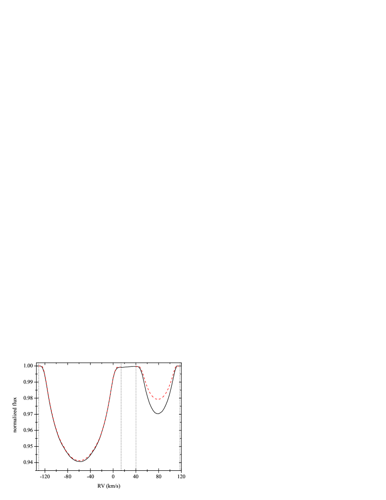
Figure 1: LSD-profile(s) of a synthetic binary system computed assuming standard (solid, black line) and multiprofile (dashed, red line) techniques. The vertical dotted lines indicate the velocity ranges for the two stars.

As already mentioned, the multiprofile LSD approach assumes that each line in the observed spectrum is represented by a superposition of N different mean profiles. According to Kochukhov et al. (2010), in that case one can still use the original matrix formulation of the LSD technique if one assumes a composite line pattern matrix of $i\times(j\cdot N)$ elements, with $N$ the number of different mean profiles. In the case of our iterative method, we simultaneously solve for $N$ different LSD-profiles spanning certain velocity ranges and characterized by different line masks which allow for diversity in atmospheric conditions. This has a practical application for binary and multiple star systems where individual stellar components can have quite different atmospheric parameters and represent their own sets of spectral lines formed under different physical conditions.

The original LSD technique introduced by Donati et al. (1997) also allows to deal with binary star systems but only with those composed of two identical stars. However, if two stars that form a binary system have different atmospheric conditions (effective temperature, surface gravity, chemical composition, etc.), an assumption of the standard LSD technique about common line mask for both stellar components appears to be incorrect. In this case, the standard method provides a potential of detecting (possibly weak) contribution of the companion star in the composite spectrum of a binary, but the depth of the (composite) average profile is largely influenced by the assumed line mask. This is illustrated in Figure 1 that compares LSD-profiles of a synthetic binary system computed assuming the standard technique as formulated by Donati et al. (1997) and a line mask of the hotter primary common for both stars (solid line), and the multiprofile technique with the difference in atmospheric conditions of the two stars taken into account (dashed lines). This difference is accounted for by using masks computed assuming different fundamental parameters for the two stars. In Figure 1, we assume $T_{\rm eff}$^1,2=8 500/7 300 K, $\log{g}$^1,2=3.4/3.5 dex, [M/H]^1,2=  0.0/-0.3 dex, $v\sin{i}$_1,2=60/30 km s^-1 for the primary and secondary, respectively, and fix microturbulent velocity to 2 km s^-1 for both stars. The average profiles are computed at phase of large RV separation assuming non-overlapping velocity grids for the two stars (indicated by the vertical dotted lines in Figure 1). Apparently, we obtain an overestimated contribution of the (cooler) secondary component when relying on the standard technique. When scaled to unity, the profiles obtained from different techniques have the same shape and deliver RVs which differ from each other by less than 100 m s^-1. In Section 5, we will come back to binary stars where, in particular, a discussion on applicability of the multiprofile LSD technique to different orbital phases will be discussed.

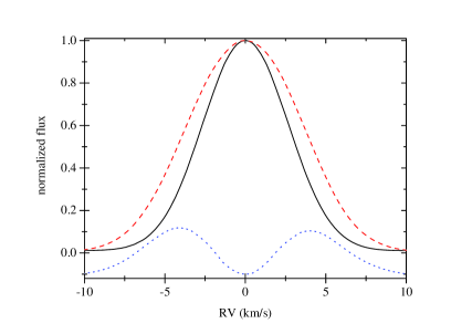
Figure 2: LSD-profiles computed for two different groups of spectral lines: with relative strengths $<0.4$ (solid, black line) and $>0.4$ (dashed, red line). The difference between the two profiles (dotted, blue line) is shown at the bottom and was shifted in Y by value of -0.1 for clarity.

The multiprofile LSD technique (to some extent) also allows to overcome one of the fundamental assumptions stating that all spectral lines in the observed spectrum are similar in shape. This assumption is justified for the majority of metallic lines in the spectrum of rapidly rotating stars as the rotational broadening clearly dominates over the other sources of broadening in this case. However, it fails for the slow rotators. Figure 2 shows normalized LSD-profiles computed for two different groups of spectral lines selected based on their theoretical relative strengths. The two profiles clearly have different shapes which can also be seen from their difference shifted to the bottom of the figure for clarity. When implementing this generalization of the standard LSD technique, one has to remember that the strengths of spectral lines in the spectrum are smoothly distributed from 0 to 1. Representation of the spectrum by a convolution of, e.g., two mean profiles with lines from the mask, where all “weak” and “strong” (below and above certain line strengths limit) lines are represented by their own LSD profile, assumes rather a step-like distribution of the line strengths. To overcome the problem of this strict division into groups with sharp edges, when solving simultaneously for $n$ mean profiles, we represent each line in the observed spectrum as a convolution of the corresponding entry from the line mask and the LSD profile computed by means of a parabolic interpolation between the $n$ mean profiles we are solving for.

Our generalization towards a multicomponent LSD profile implies that one is free to compute $N\cdot n$ average profiles at the same time, with $N$ the number of individual stellar components (two for a binary, three for a triple system, etc.) and $n$ the number of LSD-profiles per stellar component. In the calculation of the $n$ average profiles, the line weights are assigned based entirely on their relative strengths information from the mask. This implies that a pair of lines that have similar intrinsic strengths but, e.g., significantly different pressure broadening will be given (nearly) equal weights. This in turn means that besides hydrogen and helium lines, the metal lines with broad, damping wings should also be excluded from the calculations, regardless of their intrinsic strength.

Our experience shows that for moderately to rapidly rotating stars ($v\sin{i}$$>$30 km s^-1), with the rotation being dominant source of spectral line broadening, calculation of $n=2$ average profiles seems to be an optimal choice. For slowly rotating stars, calculation of the additional third LSD-profile is required to better account for the shape difference between the lines assigned to different groups. Solving for $n>3$ profiles is also possible but, in most cases, does not seem to be really feasible. In this case, the lines from the two groups representing the weakest spectral lines show negligible difference in the intrinsic shapes, and the reduced number of lines per group implies that at least one of the (probably weakest) LSD-profiles will be badly defined.

3.2 Line strengths correction algorithm

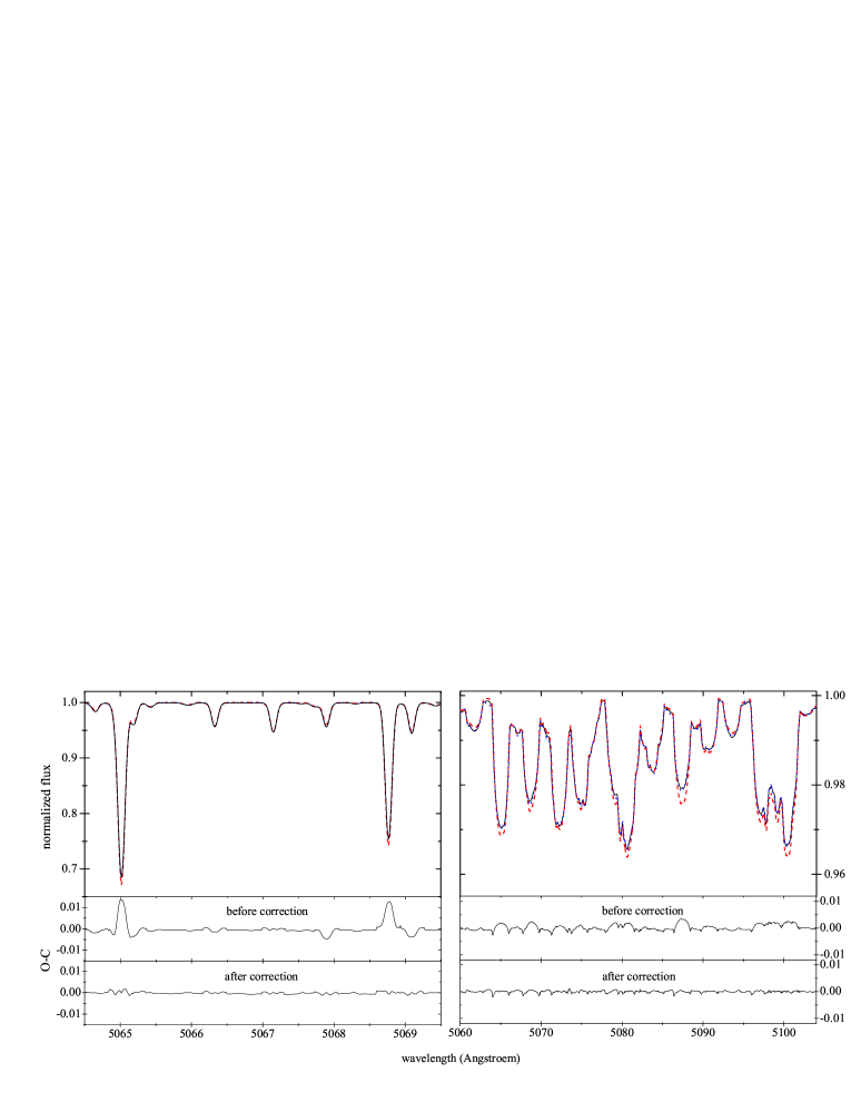
Figure 3: Comparison of the synthetic spectrum (solid, black line) with the LSD models before (dashed, red line) and after (dotted, blue line) line strengths correction. The corresponding “O-C residuals” (synthetic minus LSD-model spectrum) are shown in the middle and bottom panels. Left and right panels represent different rotation rates: $v\sin{i}$=2 km s^-1 and 60 km s^-1.

Although a convolution of $n$ mean profiles (see previous Section for definition of $n$) with lines from the mask gives a better representation of the observed spectrum than the standard technique, it is still not as good as one would like to have. The reason is obviously the second fundamental assumption of linear addition of overlapping spectral lines. As pointed out by Kochukhov et al. (2010) and has been attempted by Reiners & Schmitt (2003) in their “Physical Least-Squares Deconvolution” (PLSD), one way to overcome this limitation would be to solve simultaneously for the mean profile and individual line strengths. Sennhauser et al. (2009), on the other hand, suggest to use a non-linear line addition law of the following form:

$$R_{tot}=R_{1}+R_{2}-R_{1}\cdot R_{2},$$ (3)

where $R_{tot}$ stands for the depth of a blend formed of two individual lines with depths $R_{1}$ and $R_{2}$. The line depth $R$ is related to the line strength $r$ (to which we will refer in the subsequent sections) via the simple equation $R=1-r$. As pointed out by Kochukhov et al. (2010, Figure 4 and description therein) and verified by us, the proposed non-linear law provides a good representation of the naturally blended spectral lines with overlapping absorption coefficients. However, the residual intensities of the lines that are blended due to the limited resolving power of the instrument or due to the stellar rotation indeed add up linearly, just as the LSD technique assumes. In this case, the non-linear law proposed by Sennhauser et al. (2009) often underestimates the depth of a linearly blended line and thus appears to be inferior to the LSD description of the spectrum. The idea of solving simultaneously for the mean profile and individual line strengths would certainly be a step in the right direction but this problem is highly ill-posed and one could hardly be able to come to a unique solution. We thus decided to separate the two problems, calculation of the LSD profile and a correction of the individual line strengths, and do it iteratively until the results of both applications do not change anymore. The individual contributions are optimized “line by line” which means that only one, single line is optimized at a given instant of time, but taking into account contributions from neighbouring lines when computing the model spectrum. An exception is made for the lines with high percentage overlapping absorption coefficients, i.e. the lines which naturally locate too close to each other to be resolved by a given instrument. In other words, we define the lines as unresolved when they (naturally) locate to each other closer than it is assumed by the step width of the velocity grid on which a LSD-profile is computed. The RV step width depends on the resolving power of the instrument, and is determined directly from the observations. In this case, instead of optimizing individual line strengths, we solve for their sum accounting for theoretical percentage contribution of each individual line into the sum. Given a large number of lines we consider in our calculations, it can also happen that, according to our definition, arbitrary lines 1–2 and 2–3 are not resolved but the lines 1–3 are resolved. Moreover, a series of lines can be much longer than that and may include up to a couple of dozens of members. Our tests show that in such a case, solving for the sum of all the contributions becomes a very degenerate problem with unstable solution. Thus, in our approach, in the above mentioned three lines situation, we optimize the sum of strengths for lines 1 and 2, and then proceed with the third line, ignoring the fact that the 2–3 pair is unresolved. One can also do contrary, i.e. solve for the sum for the 2–3 pair and then proceed with the line 1, but though a certain (small) difference between the two cases can be observed during the first a couple of iterations, the end result is found to be same. During the line strengths correction, the mean profiles are normalized to unity to prevent a drifting of both the profiles and individual line strengths. The optimization algorithm can handle both single- and multi-profile LSD. In the latter case, a spectral line in the model spectrum is represented by a convolution of the corresponding entry from the mask with the average profile computed by means of (parabolic) interpolation between the $n$ components of the multiprofile LSD (see previous section for the definition of $n$). After the line strengths correction, the (multicomponent) LSD profile is recomputed based on the improved line mask, and the whole cycle is repeated until no significant changes in the profiles neither in the individual line strengths occur anymore. The efficiency of our approach will be tested and discussed in the next sections.

We use a golden section search algorithm to minimize an O–C (“Observed”–“Calculated”) function in the wavelength range determined by the shape of the LSD profile and a position of the line in question. The golden section search is a technique for finding the extremum by successively narrowing the range of values inside which the extremum is known to exist.

Our experience shows that two “global” iterations, each of which includes the calculation of the LSD profile and typically a dozen of iterations for correction of the individual line strengths, is sufficient. Figure 3 illustrates the results of the line strengths correction by comparing the initial spectrum to the two LSD models computed before and after the correction. The synthetic spectrum has been computed for $T_{\rm eff}$=8 500 K, $\log{g}$=3.4 dex, microturbulence $\xi$=2.0 km s^-1, and solar chemical composition. We consider two cases with very different rotation rates, characterized by a $v\sin{i}$ of 2 km s^-1 (top) and 60 km s^-1 (bottom). In both cases, the initial LSD model badly describes the intensity spectrum of the star while the match is nearly perfect after application of the line strengths correction algorithm.

4 Application to single stars spectra

In this section, we test our improved LSD technique on spectra of an artificial star, verify the influence of different line masks on the final results, and compare our method to the simple “running average” smoothing algorithm. The method is then applied to the spectra of the “standard” star Vega, KIC04749989, a $\gamma$ Dor-$\delta$ Sct hybrid pulsator in the $Kepler$ field, and to the spectra of 20 CVn and HD 189631, a mono-periodic $\delta$ Sct- and a multi-periodic $\gamma$ Dor-type pulsating star, respectively.

4.1 Simulated data

To test the influence of the initial model on the final results, we computed a certain number of line masks assuming different atmospheric parameters. We separately tested the impact of $T_{\rm eff}$, $\log{g}$, and [M/H], while the microturbulence was fixed to 2 km s^-1. The effect of different noise level in the “observed” spectrum is also investigated. In this section, we refer to the synthetic spectrum of an artificial star as to the “observed” spectrum for convenience.

Both, synthetic spectra and individual line strengths for the masks have been computed with the SynthV code (Tsymbal 1996) based on the atmosphere models computed with the most recent version of the LLmodels code (Shulyak et al. 2004). The information about positions of the individual lines was extracted from the VALD database (Kupka et al. 1999). We assume the star to have the same atmospheric parameters as in the previous section, i.e. $T_{\rm eff}$=8 500 K, $\log{g}$=3.4 dex, $\xi$=2.0 km s^-1, $v\sin{i}$=2.0 km s^-1, and solar chemical composition. To simulate the data of different S/N, we added Gaussian white noise to our spectra. Figure 4 illustrates a part of the “observed” spectrum assuming three different values of S/N.

The whole idea of the experiment presented here is as follows: we start with the initial “observed” spectrum, of which typically 800–1000 Å wide wavelength range free of Balmer lines is used to compute a multicomponent LSD profile as described in Section 3.1. Given that we assume only a small rotational broadening of the lines for this star, a computation of three-component average profile was found to be necessary. After a set of experiments, theoretical lines from the mask were divided into three groups, according to their predicted relative strengths: “weak” lines with individual strengths $r$ (in units of continuum) between 0 and 0.4, “intermediate” strength lines with 0.4$<$$r$$\leq$0.6, and “strong” lines satisfying condition of $r$$>$0.6. In the next step, the LSD profile is used to perform line strengths correction for the mask that has been initially used for the calculation of the mean (multicomponent) profile, and the procedure repeats until no (significant) changes in the profile nor in the individual line strengths occur. We then use the final list of the line strengths and the LSD profile to compute a model spectrum and analyse it to determine the fundamental parameters which are then compared to the originally assumed ones. For estimation of the fundamental parameters we rely on the spectral synthesis method as implemented in the GSSP (Grid Search in Stellar Parameters) code (Tkachenko et al. 2012a; Lehmann et al. 2011). The code finds the optimum values of $T_{\rm eff}$, $\log{g}$, $\xi$, $[M/H]$, and $v\sin{i}$ from the minimum in $\chi^{2}$ obtained from a comparison of the “observed” spectrum with the synthetic ones computed from all possible combinations of the above mentioned parameters. The errors of measurement (1$\sigma$ confidence level) are calculated from the $\chi^{2}$ statistics using the projections of the hypersurface of the $\chi^{2}$ from all grid points of all parameters onto the parameter in question. For this particular case, errors of measurement were estimated to be 75 K, 0.1 dex, 0.25 km s^-1, 0.7 km s^-1, and 0.08 dex in $T_{\rm eff}$, $\log{g}$, $\xi$, $v\sin{i}$, and [M/H], accordingly.

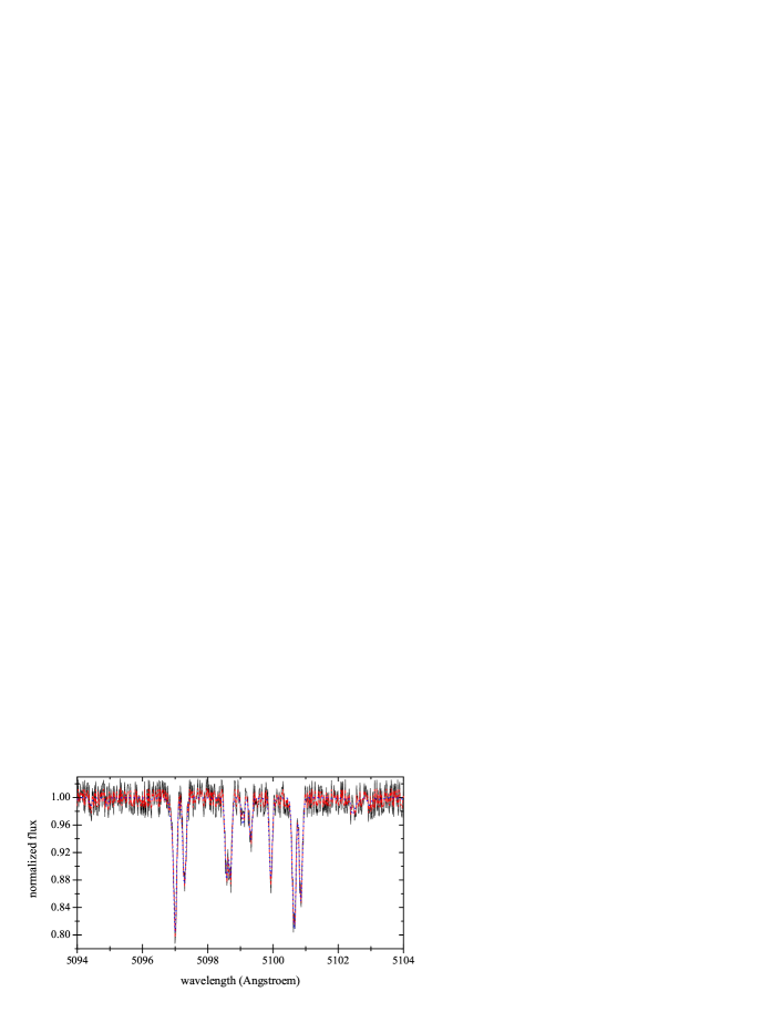
Figure 4: “Observed” spectra of an artificial star assuming different value of S/N: 35 (solid, black line), 70 (dashed, red line), and infinity (dotted, blue line)

Figure 5: Comparison between the determined and the initial model parameters for different S/N of the “observed” spectrum: infinity (open squares), 70 (open circles), and 35 (open triangles). Horizontal dashed line represents a perfect match. See text for details.

Table 1: Model parameters used for the calculation of different line masks. All models assume $\xi=$2 km s^-1. The parameter that differs from the first model is given in boldface.

model	$T_{\rm eff}$	$\log{g}$	[M/H]	model	$T_{\rm eff}$	$\log{g}$	[M/H]
	(K)	(dex)			(K)	(dex)
1	8 500	3.5	0.0	4	8 500	3.0	0.0
2	8 000	3.5	0.0	5	8 500	4.0	0.0
3	9 000	3.5	0.0	6	8 500	3.5	-0.3
				7	8 500	3.5	+0.3

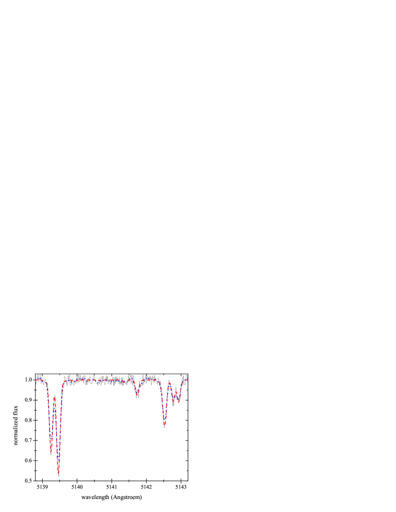
Figure 6: A few spectral features in the spectrum of a synthetic single star (solid, black line). The smoothed version of the spectrum (dotted, blue line) and the LSD model (dashed, red line) are overplotted.

Atmospheric parameters used for the calculation of the line masks range between 8 000–9 000 K with step of 500 K in $T_{\rm eff}$, 3.0–4.0 dex with step of 0.5 dex in $\log{g}$, and -0.3–+0.3 dex with step of 0.3 dex in [M/H]. Figure 5 summarizes the results in terms of a difference between the values obtained from spectral analysis of the final model spectrum and the initial parameters. The x-axis gives the model sequence number, corresponding parameters can be found in Table 1. All fundamental parameters are well reconstructed from our model spectra and individual differences do not exceed 60 K, 0.04 dex, 0.18 km s^-1, 0.5 km s^-1, and 0.05 dex in $T_{\rm eff}$, $\log{g}$, $v\sin{i}$, $\xi$, and [M/H], respectively. Such discrepancy appears to be perfectly within the estimated errors of measurement. There is also no principle difference between the spectra of different S/N values which is not of a big surprise given that there are a couple of thousands metallic lines in the considered wavelength range.

To check whether the rotation has an impact on the method and hence the final results, we repeated the whole procedure for the same type of star but assuming faster rotation with $v\sin{i}$ of 30 and then 60 km s^-1. The obtained results are the same as for the above described slowly rotating star: all reconstructed atmospheric parameters agree within the error bars with the initial values. This leads us to the conclusion that the method is robust for both slowly and rapidly rotating stars.

To verify whether the LSD-based analysis of stellar spectra is also applicable to stars with individual abundances of some chemical elements significantly deviating from the overall metallicity value, we simulated spectra of a fake stellar object assuming overabundances of Si and Mg of 0.5 and 0.2 dex, respectively. As in the previous case, we tested the method for three different values of S/N of the “observed” spectrum and checked how sensitive the technique is to the initial model by using the same line masks as for the normal star (see Table 1). The obtained results are essentially the same meaning that we can successfully reconstruct back all the fundamental parameters and individual abundances of the two chemical elements. An exception is the value of an overall metallicity which seems to be largely affected by the initially assumed overabundances of the two chemical elements and is found to be by 0.07–0.09 dex higher than the initial parameter value.

Finally, we compared our technique with a couple of widely used smoothing algorithms, like running average and median filter. These techniques are usually used to smooth out short-term fluctuations (noise in case of spectra) and highlight long-term “trends” (read, spectral features). Both techniques are equivalents of lowering spectral resolution as they assume a replacement of several neighbouring points by a single value, either average or median one. Such smoothing is justified for the spectra of constant stars with large values of projected rotational velocity. In such cases, spectral features appear to be broad and lowering resolution has no or a little influence on the derived characteristics of a star. The situation is totaly different in the case of stars exhibiting narrow lines in their spectra or/and intrinsically variable stars. In both cases, smoothing is expected to have large impact on spectral characteristics of a star, which is by artificial broadening of spectral lines in the former case and by smoothing out the pulsation signal in the latter. Indeed, Figure 6 illustrating simulated data of a slowly rotating star, clearly shows how the spectral features can be artificially broadened by smoothing algorithms. Estimated value of projected rotational velocity based on these smoothed spectra is found to be a factor of 2.5 larger than the original one. This in turn leads to incorrect values of other fundamental parameters, which is not the case when using our improved LSD algorithm.

4.2 The cases of Vega and KIC04749989

After testing the method on simulated data, we apply it to the observed spectra of Vega and KIC04749989, with the aim to check whether the obtained fundamental parameters agree with those reported in the literature. The data were obtained with the HERMES spectrograph (Raskin et al. 2011) attached to the 1.2-m Mercator telescope (La Palma, Canary Islands). The spectra have a resolving power of 85 000 and cover a wavelength range from 380 to 900 nm. The data have been reduced using the dedicated pipeline, including bias and stray-light subtraction, cosmic rays filtering, flat fielding, wavelength calibration by ThArNe lamp, and order merging. The continuum normalization was done afterwards by fitting a (cubic) spline function through some tens of carefully selected continuum points. More information on the adopted normalization procedure can be found in Pápics et al. (2012).

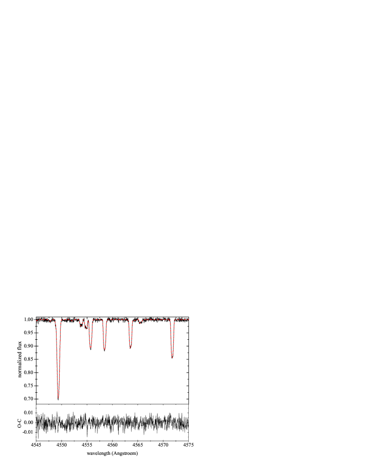
Figure 7: Comparison between the observed (solid, black line) and final LSD model (dashed, red line) spectrum of Vega.

The LSD profiles for Vega were computed from several metal line regions spread over the entire wavelength range of the HERMES spectra, and by excluding all hydrogen and helium spectral lines. Figure 7 compares two small parts of the observed spectrum of the star with the final LSD-based model obtained after the application of our line strengths correction algorithm. Similar to the results obtained for the simulated data, the model matches the observations very well and the obtained S/N is a factor of 5 higher than in the original spectrum. We used the obtained model spectrum (free of Balmer and helium lines) to estimate the fundamental parameters of the star by means of our GSSP code. Table 2 compares the atmospheric parameters of Vega obtained by us with those found by Lehmann et al. (2011) using the same atmosphere models and spectrum synthesis codes as we did. Obviously, all five atmospheric parameters are in perfect agreement with the values reported by Lehmann et al. (2011), which in turn agree very well with several recent findings for this star (see, e.g., Table 3 in Lehmann et al. 2011). It is worth noting that the errors on both $T_{\rm eff}$ and $\log{g}$ are slightly higher than those estimated by Lehmann et al. (2011). This result also seems to be reasonable as in our analysis we rely purely on metal lines, without using Balmer profiles which are a good indicator of the effective temperature and surface gravity in this temperature range.

Since we position our method as a good tool of increasing S/N of stellar spectra without losing and/or affecting relevant information, bright stars are not sufficient to test the technique on: the original observed spectrum of Vega is of S/N$\sim$300 and there is no need to improve the quality of the data to perform a detailed analysis of the star. We thus tested the method on KIC04749989, which contrary to Vega has a high value of $v\sin{i}$ of $\sim$190 km s^-1 and for which a HERMES spectrum of S/N$\sim$60 has been obtained. The high value of the projected rotational velocity for this star implies that all metal lines in its spectrum are rather weak and shallow, and show very high degree of blending.

Table 2: Comparison of the atmospheric parameters of Vega obtained by us with those reported by Lehmann et al. (2011). Errors of measurement estimated from $\chi^{2}$ statistics and represented by 1-$\sigma$ level are given in parenthesis in terms of last digits.

Parameter	Unit	This paper	Lehmann et al. (2011)
$T_{\rm eff}$	K	9 500 (140)	9 540 (120)
$\log{g}$	dex	3.94 (12)	3.92 (7)
$v\sin{i}$	km s-1	22.3 (1.2)	21.9 (1.1)
$\xi$	km s-1	2.20 (40)	2.41 (35)
${\rm[M/H]}$	dex	–0.60 (12)	–0.58 (10)

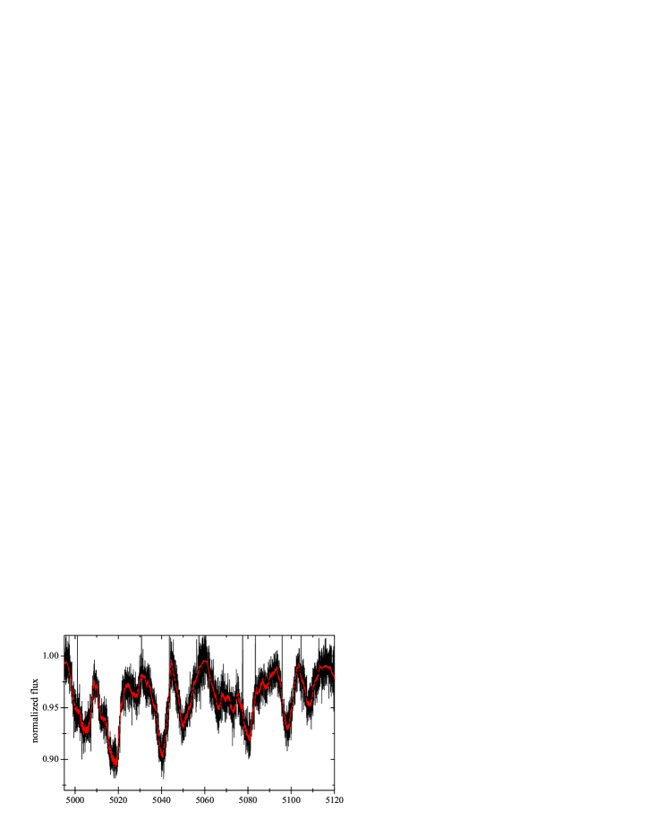
Figure 8: Same as Fig. 7 but for KIC04749989.

For the calculation of the LSD profile and the corresponding model spectrum, we used the wavelength region rich of metal lines, from 495 to 580 nm. Figure 8 illustrates a part of the observed spectrum of KIC04749989 (solid, black line) and compares it with our final LSD-based model spectrum (dashed, red line). The latter has S/N of $\sim$700 implying a gain by a factor of 10 compared to the original data. To check the impact of the observational noise on the fundamental parameters estimate, both the original and the LSD-based model spectra were analysed with the GSSP code in the same, above mentioned wavelength region. Table 3 compares the results revealing rather large discrepancies between the two sets of obtained parameters. Indeed, there is a difference of about 400 K and 0.3 dex in the effective temperature and surface gravity, respectively, as well as non-significant difference of 6 km s^-1 in $v\sin{i}$. As expected, the rather high noise level in the original data has large impact on the derived fundamental parameters which is also confirmed by the large error bars. On the other hand, at least one properly normalized Balmer profile significantly helps in constraining both $T_{\rm eff}$ and $\log{g}$, which in turn leads to a more precise estimation of the two other parameters. Indeed, the same observed, low S/N spectrum of KIC04747989 was analysed by Tkachenko et al. (2013), but using a wider wavelength range from 470 to 580 nm, that, besides metal lines, also covers the H_β profile. The corresponding fundamental parameters are listed in the last column of Table 3 and agree very well with those derived by us from the high S/N LSD-based model spectrum. Normalization of Balmer lines in noisy spectra is far from trivial and is an additional source of uncertainties in the derived $T_{\rm eff}$ and $\log{g}$. Our method does not rely on Balmer lines but is fully based on fitting the metal lines wavelength regions, and thanks to the significantly improved S/N of spectra, delivers appropriate results.

Though there is no obvious advantage in using our proposed LSD-based method for stars like Vega for which good quality data could be obtained even with very small telescopes, the method promises to be very robust for faint stellar objects (primary targets of, e.g., the $Kepler$ spacecraft) observed with 1 to 2-m class telescopes. Given that our LSD model spectra contain all relevant information present in the original, observed spectra but provides much better S/N data, the technique should also have its practical application to intrinsically variable (e.g., rotationally modulated and/or pulsating) stars. Thus, in the next Section, we investigate the robustness of our method for pulsating stars, by testing it on high-resolution spectra of 20 CVn and HD 189631, two well-studied $\delta$ Sct and $\gamma$ Dor-type pulsators.

4.3 Asteroseismic targets: the cases of 20 CVn and HD 189631

As long as a star shows pulsations, asteroseismology, the study of stellar interiors via interpretation of pulsation patterns observed at the surfaces of the stars, allows for extremely accurate estimation of fundamental stellar parameters like mass, radius, density, etc. Knowledge of these parameters is in turn of major importance for understanding stellar evolution as well as for the correct characterization of exoplanets and their interaction with host stars. Nowadays, in the era of the MOST (Microvariability and Oscillations of STars, Walker et al. 2003), CoRoT (Convection Rotation and Planetary Transits, Auvergne et al. 2009) and $Kepler$ (Gilliland et al. 2010) space missions providing us with micro-magnitude precision photometric data for numerous pulsating stars, we still lack additional information to perform in-depth asteroseismic studies for many of those stars. Indeed, the above mentioned missions observe their targets in white light which makes identification of individual pulsation modes, one of the pre-conditions for asteroseismology to work, impossible from these data unless one can identify the modes from frequency or period patterns alone. This is usually the case for stochastically excited modes in the asymptotic acoustic regime or for high-order gravity mode pulsations, but not in general for heat-driven modes (e.g., Aerts et al. 2010). For the latter, one needs extra information in terms of time-series of (ground-based) multicolour photometry and/or high-resolution spectroscopy to be obtained. A combination of the high-resolution but moderate S/N spectra obtained with lower class telescopes and our new technique, may provide data of sufficient quality to perform the desired analysis.

In this section, we test our method on 20 Canum Venaticorum and HD 189631, a bright ($V$=4.73) $\delta$ Sct-type pulsator and a non-radially pulsating $\gamma$ Dor star, respectively. Our ultimate goal is to check whether the LSD-based model spectra providing a much higher S/N compared to the original data, at the same time, do not affect the oscillation signal present in the original spectra in terms of LPV. This is done by extracting individual frequencies from the time-series of the LSD model spectra and performing identification of the individual oscillation modes. The results are then compared to those obtained from the original data as well as to the results of previous studies. In both cases, we make use of the FAMIAS software package (Zima 2008) for the extraction of the individual frequencies as well as for the mode identification. The analysis is based both on the moment (Aerts et al. 1992; Briquet & Aerts 2003) and pixel-by-pixel (Zima 2008) methods.

Table 3: Comparison of the atmospheric parameters of KIC04749989 obtained by us from the original data and from the LSD-based model spectrum with those reported by Tkachenko et al. (2013, indicated as T2013). The latter study made use of the H_β profile to put additional constraints on $T_{\rm eff}$ and $\log{g}$, and is used here as a reference. Errors of measurement estimated from $\chi^{2}$ statistics and represented by 1-$\sigma$ level are given in parenthesis in terms of last digits.

Parameter	Unit	This paper		T2013
		Original	LSD model
$T_{\rm eff}$	K	6 950 (200)	7 380 (130)	7 320 (120)
$\log{g}$	dex	4.02 (45)	4.34 (25)	4.32 (35)
$v\sin{i}$	km s-1	184 (10)	190 (8)	191 (10)
$\xi$	km s-1	2∗	2∗	2∗
${\rm[M/H]}$	dex	+0.12 (12)	–0.03 (8)	+0.00 (12)
∗ fixed

4.3.1 20 Canum Venaticorum

Periodicity of 20 CVn was discovered by Merrill (1922) who reports it to be a binary candidate. However, Wehlau et al. (1966) noticed this misclassification of the star as a binary and propose the $\delta$ Sct-type oscillations as the cause of the observed variability. Since then, 20 CVn was the subject of several photometric and spectroscopic studies which led to a large diversity in results and interpretations. For example, Shaw (1976) finds the star to be a mono-periodic $\delta$ Sct pulsator whereas Smith (1982) and Bossi et al. (1983) report the detection of a second oscillation mode. The same holds for the proposed type of oscillations where, for instance, Mathias & Aerts (1996) classify the star as a non-radial pulsator whereas Rodriguez et al. (1998) report on the radial identification for the observed pulsation mode. The conclusions by Rodriguez et al. (1998) were later on confirmed by Chadid et al. (2001) and Daszyńska-Daszkiewicz et al. (2003). The atmospheric parameters are also not very well constrained for this star revealing a scatter in the literature of about 700 K, 0.7 dex, and 10 km s^-1 in $T_{\rm eff}$, $\log{g}$, and $v\sin{i}$, respectively (see, e.g., Hauck et al. 1985; Rodriguez et al. 1998; Erspamer & North 2003). This particular diversity in the reported fundamental parameters provides an excellent test of our technique and, in particular, allows to check an impact of the selected line mask on the final results.

We base our analysis on spectra taken with the ELODIE échelle spectrograph, at the time of its operation (1993–2006) attached to the 193-cm telescope at Observatoire de Haute-Provence (OHP). The data have a resolving power of 42 000, cover wavelength range from 3895 to 6815 Å, and were originally obtained by Mathias & Aerts (1996), Chadid et al. (2001), and Erspamer & North (2003). We used the ELODIE archive (Moultaka et al. 2004) to retrieve the data, Table 4 gives the journal of observations listing the source, the period of observation, number of the acquired spectra, and the average S/N value.

The ELODIE archive contains pre-extracted, wavelength calibrated spectra. Besides the continuum normalization and correction for the Earth’s motion, we carefully examined the spectra for any additional systematic nightly RV variations. The variability of the order of 100-300 m s^-1 was detected, in perfect agreement with the findings by Chadid et al. (2001). These authors attribute this variability to instabilities of the ELODIE spectrograph, more specifically, of the ThAr spectra served to calibrate the spectral wavelength scaling. Following the procedure proposed by Chadid et al. (2001), we corrected the spectra from each night by matching the corresponding (nightly) mean RV to the mean value observed in 1998.

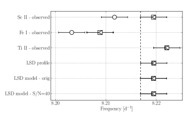
Figure 9: Comparison of the frequencies extracted from the three different spectral lines in the original observed spectra of 20 CVn with the values deduced both from the LSD-based model spectra (for the Sc II 5239 Å only, based on the data sets characterized by different S/N) and the LSD profiles themselves. The symbols refer to the three observables used for the analysis: the first- and the third-order moment (squares and circles, respectively), and the profiles themselves (triangles). The frequency errors are assumed to correspond to the Rayleigh limit of the data. The vertical dashed line represents the literature value of 8.2168 d^-1 (Rodriguez et al. 1998).

Table 4: Journal of observations for 20 CVn and HD 189631. Besides the original source and the period of observations, we list the number of obtained spectra ($N$) and the average value of S/N.

Source	Observing period	$N$	S/N
20 CVn
Mathias & Aerts (1996)	20–21.12.1994	8	84
Chadid et al. (2001)	11–15.04.1998	113	127
	24–25.04.1999	31	168
	27–30.04.1999	131	126
Erspamer & North (2003)	05–06.06.1999	1	308
Unknown	28–29.03.2002	1	260
HD 189631
Maisonneuve et al. (2011)	02–09.07.2008	274	215
	22.06–02.07.2009	24	165
	17–21.07.2009	25	360

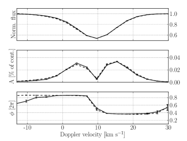
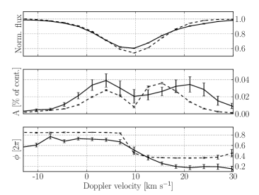
Figure 10: Results of the frequency analysis of Sc II 5239 Å line in the spectra of 20 CVn by means of the pixel-by-pixel method. The two panels stand for the original data (left) and the simulated data set characterized by S/N of 40 (right). Each panel illustrates the mean profile (top), and the amplitude and phase across this profile (middle and bottom, respectively). The solid and dashed lines represent the original observed and the LSD-based model spectra, respectively. The corresponding error margins are shown by the bars. The results are shown for the dominant (radial) mode of $\sim$8.22 d^-1 (95.11 $\mu$Hz).

As can be seen from the last column of Table 4, the original data are of rather good quality and have an average S/N above 100. In order to test the influence of the noise on the final results, we created an additional data set by adding noise to the original spectra of 20 CVn to simulate S/N of 40. Both data sets were subject for frequency analysis which was performed based on three rather strong and weakly blended spectral lines: Sc II 5239 Å, Fe I 5288 Å, and Ti II 5336 Å. The obtained results were then used for comparison with both the literature and the results obtained from the LSD-based model spectra. The latter were computed from both data sets (original and those with S/N of 40), assuming a line mask characterized by $T_{\rm eff}$=7 600 K, $\log{g}$=3.6 dex, and [M/H]=+0.5 dex, the parameters reported by Rodriguez et al. (1998). We based our analyses on the pixel-by-pixel method and on the first and the third moments of the line profiles, whereas we were unable to detect any significant variability in their second moment.

Table 5: Results of the frequency analysis for HD 189631. The values obtained by Maisonneuve et al. (2011) are given for comparison. The Rayleigh limit amounts to 10^-3 d^-1 and 10^-5 d^-1 for the data used in this paper and those of Maisonneuve et al. (2011), respectively. $\langle v\rangle$, $\langle v^{3}\rangle$, and PBP stand for the first and the third moments, and the pixel-by-pixel method, respectively.

Freq.	Unit	Maisonneuve et al.	Identification		This paper			Identification
		(2011)	$l$	$m$	$\langle v\rangle$	$\langle v^{3}\rangle$	PBP	$l$	$m$
f1	d-1 ($\mu$Hz)	1.6719 (19.3439)	1	1	1.682 (19.461)	1.682 (19.461)	1.685 (19.495)	1	1
f2		1.4200 (16.4294)	1	1	1.382 (15.990)	1.382 (15.990)	1.411 (16.325)	1	1
f3		0.0711 (0.8226)	2	–2	0.119 (1.377)	0.127 (1.469)	0.122 (1.412)	—	—
f4		1.8227 (21.0886)	4	1	1.823 (21.092)	1.820 (21.057)	1.826 (21.127)	1	1
			or
			2	–2

The results obtained from the LSD-based model spectra were essentially the same for all the three above mentioned spectral lines, as they were the same from the analysis of average profiles themselves. For this reason, from this point on, we focus on the results obtained for the Sc II 5239 Å spectral line only but the conclusions are valid for the two other lines and for the average profiles. Figure 9 compares the frequencies obtained from the analysis of all the three lines in the original observed spectra with those deduced from the LSD profiles themselves as well as from the LSD-based model of the Sc II 5239 Å line. As expected, the frequency obtained from the analysis of this line in the LSD model spectra matches well the one deduced from the average profiles themselves. This is because all the information about LPV that is present in the LSD-model spectra entirely comes from the average profiles extracted directly from the observations. Our decision to work here with several individual lines from the LSD spectra but not with the mean profiles themselves is due to interest to what extend the noise can influence results of the frequency analysis when applied to different observables. In Figure 9, one can see that frequencies extracted from the LSD model spectra (whatever the S/N value is assumed) using different diagnostics (pixel-by-pixel or spectral line moments) are in perfect agreement with each other and with the value reported by Rodriguez et al. (1998) (vertical dashed line). On the other hand, being applied to the original spectra, frequency analysis of the third-order moment of the line (open circle in the top most line in Figure 9) reveals different results from those obtained by pixel-by-pixel and the first-order moment methods. Since the degree of blending of this particular spectral line of Sc II at 5239 Å is the same both in the original and LSD model spectra, we conclude that the above mentioned difference in the extracted frequencies is purely due to noise present in the original data. We also find that the Fe I 5288 Å, and Ti II 5336 Å lines from the original observed spectra deliver slightly different results, but this can be explained by the higher degree of blending and effects of normalization to the local continuum for these two lines. Finally, we stress that both the moment and pixel-by-pixel methods applied to the LSD model spectra or the average profiles themselves lead to consistent results for this star (see different symbols in Figure 9).

Figure 10 illustrates the results of the frequency analysis of the Sc II 5239 Å line by means of the pixel-by-pixel method, based on both the observed and the LSD-based model spectra and assuming two different data sets: original (left) and simulated, characterized by S/N of 40 (right). Each panel contains three subplots showing the mean profile, and the amplitude and phase variations corresponding to the determined frequency of 8.2195 d^-1 (95.0996 $\mu$Hz). The solid and dashed lines refer to the observed and LSD model data, respectively, the corresponding error margins are indicated by the bars. One can see that the resulting mean profile as well as the amplitude and phase measured across this profile are all strongly affected by the noise present in the observations (solid lines and associated with them errors in the right panel). This implies that the obtained observables based on the spectra of S/N$=$40 cannot be used for further analysis and, in particular, identification of individual oscillation modes. On the other hand, the LSD-based model spectra computed from the same observations provide us with much more accurate measurements which appear to be in a good agreement with those obtained from the original, high S/N data (left panel) and are thus well suitable for further mode identification. Indeed, the identification of the dominant oscillation mode of 8.2195 d^-1 (95.0996 $\mu$Hz) suggests it to be either a radial mode or $l=1$ zonal mode. The latter identification is favoured by the moment method providing slightly lower reduced $\chi^{2}$ value, while the former identification as a radial mode is found to be the most probable when relying on the pixel-by-pixel method. This finding is in perfect agreement with the previous studies by, e.g., Rodriguez et al. (1998) and (Aerts et al. 2010, Chapter 6).

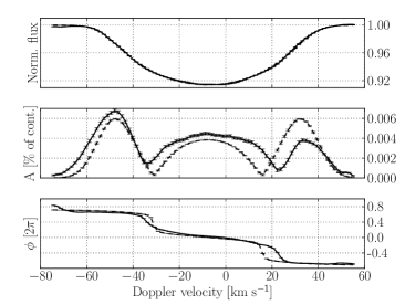
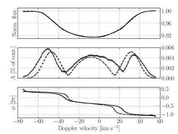
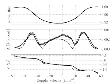
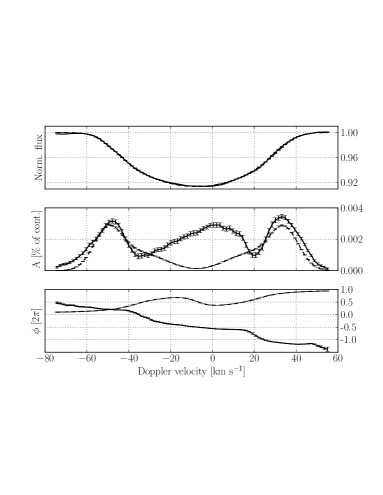
Figure 11: Results of the mode identification by means of the pixel-by-pixel method for the three (out of four) frequencies detected in the spectra of HD 189631: f₁ (top left), f₂ (top right), and f₄ (bottom). The bottom left and right panels stand for the $(l,m)=(1,1)$ and $(l,m)=(2,-2)$ identifications, respectively. The solid and dashed lines stand for the observations (LSD spectra) and the (FAMIAS) model, respectively. Both the frequency values and their identifications are listed in Table 5.

4.3.2 HD 189631

HD 189631 is a bright ($V$=7.54), late A-type $\gamma$ Dor non-radial pulsator. We chose this object to test our LSD method on for the two reasons: i) this star is one of a few $\gamma$ Dor-type pulsators for which an extensive spectroscopic mode identification study has been conducted (Maisonneuve et al. 2011), and ii) more than 300 high-resolution spectra obtained by Maisonneuve et al. (2011) with the HARPS échelle spectrograph attached to the ESO’s 3.6-m telescope (La Silla, Chile) were publicly available through the ESO Science Archive. The obtained data were already pre-extracted and wavelength calibrated, and additionally normalized to the continuum by us. Table 4 gives the journal of observations listing the observing period, the number of the obtained spectra, and the average S/N.

Having an independent mode identification was important for us because the star is a moderate rotator ($\sim$45 km s^-1, Maisonneuve et al. 2011) showing a large number of metal lines in its spectrum, which provides a high degree of blending making mode identification based on single observed line profiles a very difficult task. Thus, we used the original observed spectra to compute the LSD profiles and analysed the latter to determine frequencies and identification of the individual pulsation modes. In the previous Section we showed that i) the LSD profiles deliver essentially the same results as the LSD model spectra, and ii) the noise level in the original spectra has no impact on the final results and their interpretation given that sufficient number of metallic lines are available for calculation of the average profile. Thus, for this particular star, we restricted our analysis to the LSD profiles only, computed for the original, high S/N ratio spectra, and aimed to check whether the LSD-based analysis is also suitable for multi-periodic, non-radially pulsating stars.

We compare our results to those reported by Maisonneuve et al. (2011). As such, it is worth noting that these authors benefitted from additional spectroscopic data obtained with the HERCULES and FEROS spectrographs operated at the Mount John University Observatory (MJUO, New Zealand) and European Southern Observatory (ESO, Chile), respectively. In practice, Maisonneuve et al. (2011) had a longer time base of the observations which in turn transforms into a higher frequency resolution. Similar to the case of 20 CVn, we base our analysis on both the moment and the pixel-by-pixel methods. The results of the frequency analysis are summarized in Table 5. Similar to Maisonneuve et al. (2011), we detected four individual frequency peaks, all in the typical $\gamma$ Dor stars low-frequency domain. Despite the fact that we had less data at our disposal, the frequency values obtained by us by (at least) one of the methods compare well to those reported by Maisonneuve et al. (2011), except for the f₃ mode. Thus, we focused on the three modes f₁, f₂, and f₄, and performed a simultaneous mode identification for them. We have found that all the three modes are probably $l$=1 sectoral modes, the results for f₁ and f₂ are consistent with the findings by Maisonneuve et al. (2011). The identification for f₄ is different from the one presented by these authors, but it is worth noting that the $(l,m)=(2,-2)$ geometry appears to be second best solution in our calculations (the solution proposed by Maisonneuve et al. (2011) as a possible one, see Table 5).

Figure 11 illustrates the results of the mode identification for all the three frequencies by showing the fit to the mean profiles, and the amplitude and phase variations. For the highest frequency mode f₄, we present two identifications, of which one corresponds to our best solution dipole mode (bottom left), while the second one stands for $l=2$ retrograde sectoral mode (bottom right) proposed by Maisonneuve et al. (2011) as one of the possible solutions. Clearly, $l=2$ mode does not allow to fit neither the observed amplitude nor phase variations across the profile, with the largest discrepancy for the amplitude being in the center of the line. The $(l,m)=(4,1)$ solution proposed by Maisonneuve et al. (2011) for this mode, though not shown here, was also found by us as one of the possible identifications. However, we find it unlikely that f₄ is $(l,m)=(4,1)$ mode because (i) according to the obtained $\chi^{2}$ values, this solution appears to be twice as bad as the dipole mode, and (ii) the obtained inclination angle is close to the so-called inclination angle of complete cancelation (IACC, e.g., Chadid et al. 2001; Aerts et al. 2010), which stands for the angle at which a particular mode becomes undetectable in the integrated light due to geometrical cancelation effect. Thus, we conclude that similar to the two highest amplitude modes f₁ and f₂, the f₄ mode is most probably a $l=1$ sectoral mode.

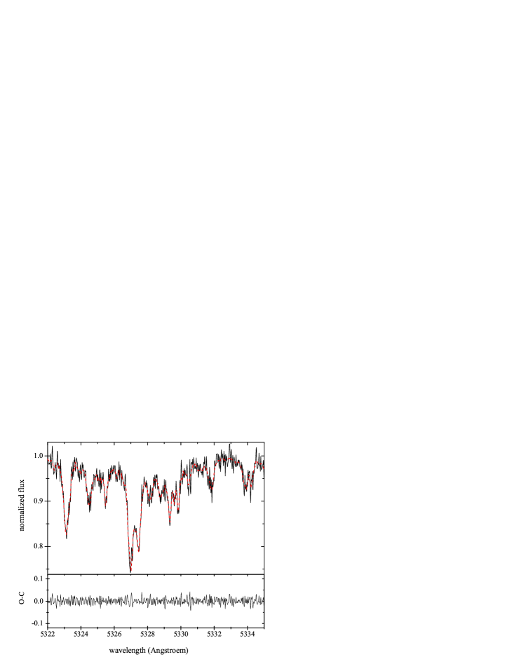
Figure 12: Same as Fig. 7 but for KIC 11285625.

The fact that all the three modes are found to have the same spherical degree $l$ suggests that these might be members of either rotationally splitted multiplet or (non)uniform period spacing of gravity modes (for detailed description of both effects, see e.g. Aerts et al. 2010). Rotationally splitted modes tend to have the same degree $l$ but different azimuthal number $m$ and the value of splitting allows to deduce the rotational period of the star. Thus, we checked whether at least one of the three considered here oscillation modes could be characterized by negative value of $m$, that is, being a retrograde mode. From the modelling, we find that for all the three modes, negative sign for azimuthal number $m$ suggests either nearly zero amplitude in the center of the line or increasing phase across the profile (similar to what is shown by the dashed line in the bottom right panel of Figure 11). This contradicts the observed characteristics of the modes, as all of them show decreasing phase and exhibit significant amplitudes in the line center (cf. Figure 11). Thus, we conclude that the three modes have positive $m$ values and cannot be the members of a rotational multiplet. On the other, the first-order asymptotic approximation for non-radial pulsations predicts the periods of high-order g-modes to be equally spaced (Tassoul 1980; Aerts et al. 2010). That is, low-degree gravity modes characterized by the same $l$ and $m$ numbers but different radial orders $n$ may form multiplets of equidistantly spaced in period peaks. The spacings can also be non-equidistant if, e.g., the chemical composition gradient exists near the stellar core (e.g., Miglio et al. 2008; Degroote et al. 2010). The two of the detected and identified in this work as $(l,m)=(1,1)$ modes of HD 189631, f₁ and f₂, show the period spacing which is $\sim$2.5 times larger than the spacing between f₁ and f₄ modes. The latter spacing of $\sim$3 900 s seems to be well in the range of theoretically predicted spacings of $l=1$ modes for a typical $\gamma$ Dor-type pulsator. Thus, we speculate that the three modes f₁, f₂, and f₄ might show non-equidistant period spacing, but also stress that an in-depth (theoretical) analysis is needed to prove that. This kind of analysis is beyond the scope of the current paper.

5 Composite spectra of binary stars

As discussed in Section 3, the multiprofile technique, in particular allows to account for difference in atmospheric conditions of the two stars forming a binary system by assuming two different sets of spectral lines in a mask. With a proper mask choice, similar to the case of single stars, our improved LSD technique has a potential of good representation of a binary composite spectrum and thus, its effective denoising.

For spectroscopic double-lined binaries, determination of fundamental parameters of both components is usually achieved by means of the spectral disentangling technique (Simon & Sturm 1994; Hadrava 1995). The method requires a good orbital phase coverage and delivers mean decomposed spectra that can be analysed by means of the tools suitable for single stars. One also benefits in S/N, the gain is proportional to $\sqrt{N}$ (additionally scaled to the light ratio of the two stars), with $N$ the number of individual composite spectra. With only a few rather noisy (but well sampled in orbital phase) composite spectra, the gain in S/N is usually not sufficient to conduct the desirable analysis. For example, this was the case for KIC 11285625, a spectroscopic double-lined eclipsing binary with a $\gamma$ Dor-type pulsating primary component. Due to the originally noisy composite spectra and a small contribution of the secondary component to the total light of the system, the resulting decomposed spectrum of the secondary was of insufficient S/N to determine spectral characteristics of this star (Debosscher et al. 2013). Given that both components of this binary system are slow rotators showing large number of spectral lines in their spectra, our denoising technique should be very robust in this case. Figure 12 illustrates two portions of the observed composite spectrum of KIC 11285625 along with the best fit LSD model spectrum. A three-component average profile was computed for each stellar component of this binary system, which means that we solved for 2$\times$3=6 LSD profiles simultaneously. The line masks for both stars were computed using the SynthV spectral synthesis code (Tsymbal 1996) and assuming effective temperature and surface gravity values of $T_{\rm eff}$^1,2=6950/6400 K and $\log{g}$^1,2=4.0/4.2 dex for the primary and secondary, respectively (Debosscher et al. 2013). Given a low S/N of the spectrum of the secondary component obtained in that work, effective temperature of this star was estimated from the relative eclipse depths. Similar to the case of KIC 4749989 (cf. Section 4), spectrum recovery for KIC 11285625 is very good and a gain in S/N is a factor of 10 compared to the original data. The high S/N LSD spectra can further be used for spectral disentangling and ensure high S/N for the resulting decomposed spectrum of the secondary. The latter in turn can be used to determine the fundamental parameters and chemical composition of the star.

In a similar way, our technique has been used to look for the signatures of the secondary component in the (noisy) observed spectra of a red giant star KIC 05006817 (Beck et al. 2013). Using the improved LSD technique, the authors could conclude that the star is a single-lined binary, estimating the detection limit of the spectral features of the secondary in the composite spectra to be of the order of 1% of the continuum.

Similar to the Section 3 dedicated to our improvements of the original LSD method, we applied out technique to the binary spectrum taken at the orbital phase of large RV separation. In practice, this means that the individual mean profiles are computed from non-overlapping RV grids, which provides their effective deconvolution. A few additional tests that we conducted on synthetic binary spectra characterized by a small RV separation of the two stars reveal that the resulting individual mean profiles both show a contribution of the primary and secondary components. In other words, the LSD method suffers from degeneracy between spectral contributions of the two stars when the average profiles are computed on (largely) overlapping RV grids. Though the RVs derived from such mean profiles can be associated with rather large uncertainties, our line optimization method seems to work well also at orbital phases of small RV separation, providing reasonably good recovery of the original spectrum. Especially, this is the case when the two stars show considerably different line broadening in their spectra (have significantly different $v\sin{i}$ values). However, we would expect our method to fail completely in eclipse phases, where besides (nearly) zero RV separation of the stars, spectral lines of one of the components can be remarkably distorted due to the Rossiter-McLaughlin effect (Rossiter 1924; McLaughlin 1924).

6 Discussion and Conclusions

The MOST, CoRoT, and $Kepler$ space-missions photometric data are of unprecedented quality and led to a discovery of a large number of intriguing objects (the stars hosting exoplanets, pulsating and binary stars, etc.). For an efficient characterization of all those diverse stellar objects, we still need ground-based support observations in terms of high-resolution spectroscopy and/or multicolour photometry. The majority of the objects are faint implying that they either have to be observed with large telescopes providing sufficiently high S/N for the desired analysis, or a technique allowing to gain in S/N for the spectroscopic data obtained with 2-m class telescopes is required. Thus, we dedicated this paper to the development of such a technique, which is based on the method of Least-Squares Deconvolution originally proposed by Donati et al. (1997).

We presented a generalization of the original LSD technique by reconsidering its two fundamental assumptions on self-similarity of all spectral lines and their linear addition to build the spectrum. Following Kochukhov et al. (2010), we implemented a multicomponent LSD profile implying representation of the observed spectrum as a superposition of several average profiles computed for different line groups. The latter can be formed, e.g., according to the strengths of individual lines, by subdividing the lines according to the corresponding chemical elements (e.g., roAp or CP stars) and/or stellar objects (the case of multiple stars), etc. We also introduced a line strengths correction algorithm that minimizes the effect of non-linear addition of spectral lines in a spectrum and provides a good representation of the observations. The resulting LSD model spectrum is of high S/N and contains all the information from the original, observed spectrum. However, we stress that the optimized individual line strengths hardly have their original physical meaning, as the problem of non-linear addition of lines with overlapping absorption coefficients requires a solution of radiative transfer and cannot be solved by our simple line strength optimization routine.

The method was first tested on simulated data of a fake stellar object assuming three different values of S/N: infinity, 70, and 35. We also checked the sensitivity of the technique to the chosen line mask that in addition to the line positions contains an information on their relative strengths. For calculation of the line masks, we varied $T_{\rm eff}$, $\log{g}$, and [M/H] in $\pm$500 K, $\pm$0.5 dex, and $\pm$0.3 dex windows, respectively, and found that in all the cases, our technique provides a good representation of the original observed spectrum. The corresponding LSD model spectra were then analysed to determine fundamental parameters by means of the spectral synthesis method. The initially assumed parameter values could always be efficiently reconstructed from the LSD model spectra with the deviations from the original values of $\sim$50 K in $T_{\rm eff}$, $\sim$0.05 dex in both the metallicity and $\log{g}$, $\sim$0.5 km s^-1 in $v\sin{i}$, and $\sim$0.18 km s^-1 (the case of significantly wrong metallicity, while the typical deviation is $\sim$0.06 km s^-1) in microturbulent velocity being the worst.

The method was then applied to the observed spectra of Vega and a $Kepler$ target, KIC04749989. Similar to the tests on simulated data, the observed spectrum of Vega was successfully reproduced by our LSD model and the derived fundamental parameters were found to be in a good agreement with the recent findings from literature. Since the method is certainly not aimed for application to the bright stars like Vega for which a high-quality spectrum can be obtained even with small telescopes, it was applied to a faint target KIC04749989 for which a high-resolution but low S/N of $\sim$60 spectrum existed. We found that such high noise level has a large impact on the derived fundamental parameters when the original observed spectrum is used for the analysis, but that a gain in S/N by a factor of more than 10 overcomes this problem, and the corresponding LSD model delivers appropriate for that star atmospheric parameters.

A large number of faint pulsating stars discovered by, e.g., $Kepler$ space mission, nowadays requires ground-based support (spectroscopic) observations to make the identification of the individual pulsation modes possible for those stars. Thus, we tested our method on the two pulsating stars, 20 CVn and HD 189631, each one oscillating in different types of modes, to check whether the technique is also applicable to the intrinsically variable stars and what kind of impact it might have on the pulsation content in the spectrum, if any. We have found that in both cases the results are very satisfactory and are in perfect agreement with those found in the literature. In particular, we could show that 20 CVn is a $\delta$ Sct-type mono-periodic pulsator, most likely, oscillating in a radial mode. These results were found to be consistent with the findings by, e.g., Rodriguez et al. (1998), Chadid et al. (2001), and Daszyńska-Daszkiewicz et al. (2003). HD 189631 was in turn proved to be a multi-periodic $\gamma$ Dor-type pulsator, with all the three dominant frequencies being identified as $l$=1 sectoral modes. The findings for the two dominant modes, f₁ and f₂, are compatible with the recent results obtained by Maisonneuve et al. (2011) based on high-resolution spectroscopic data. We also showed that the identification presented by these authors for the third dominant mode f₄ is in considerable disagreement with the observations, which are in turn best represented by $l=1$ prograde sectoral mode. We speculate that the three mode might show non-equidistant period spacing of g-mode but more (theoretical) effort is required to prove this.

We compared the LSD method with the two widely used smoothing algorithms, running average and median filter. We found that the latter are appropriate for constant stars with large projected rotational velocities, so that lowering the originally high ($>$50 000) resolving power of the spectrum has no impact on the spectral characteristics derived from it. For slowly rotating and/or intrinsically variable stars, the smoothing algorithms allow to increase S/N of the spectra but deliver unreliable results. For example, for sharp-lined stars, smoothing introduces artificial line broadening which has an impact on all fundamental parameters, while for the pulsating stars, it reduces the amplitude of or even completely removes the pulsation signal. Our LSD method does not reveal these problems and can be applied to both fast and slow rotators as well as to the intrinsically variable stars.

Although the LSD method is expected to be the most effective for G- to early A-type stars showing a lot of metal lines in their spectra, it is not limited to these objects. It can also be applied to hotter B-type stars given that large enough wavelength coverage is provided. Though we did not test the method on these type of objects in this paper, there are quite a few examples where the LSD technique was successfully applied to hotter stars with the aim to look for binary and/or spot signatures as well as to detect magnetic fields (e.g., Petit 2011; Kochukhov et al. 2011; Kochukhov & Sudnik 2013; Tkachenko et al. 2012b; Aerts et al. 2013).

Application to the spectrum of KIC 11285625, a double-lined spectroscopic binary, showed that the technique also allows effectively denoise composite spectra of binary stars. In future papers, we plan to continue development of the method and to implement an algorithm of disentangling of binary spectra based on the LSD profiles. Currently, it is impossible to do as our simple line optimization algorithm suffers from strong degeneracy between contributions of individual stellar components and delivers unreliable disentangled spectra. However, at its present stage, the method can also be effectively combined with the existing techniques of disentangling of binary spectra. That is, one can apply the LSD method to denoise composite spectra of a binary star and then to disentangle the spectra of individual stellar components by means of a disentangling technique in Fourier space (Hadrava 2004; Ilijic et al. 2004). KIC 05006817, a red giant star in an eccentric binary system, is one example of such simultaneous application of the two methods (for details, see Beck et al. 2013). A complementary approach is to use the LSD profiles themselves for accurate radial velocity measurements of spectroscopic binary and triple systems Hareter et al. (2008).