STEPWISE SYNTHESIS OF CONSTRAINED CONTROLS FOR SINGLE INPUT NONLINEAR SYSTEMS OF SPECIAL FORM

Abstract

The controllability problem for nonlinear control systems with one-dimensional control of the form $dx/dt=a(x)+B(x)\beta(x,u)$ is considered, where $a(x)$ is an $n$-dimensional vector function, $B(x)$ is an $(n\times m)$-matrix, and $\beta(x,u)$ is an $m$-dimensional vector function. Under certain conditions we reduce such system to a system consisting of $m$ subsystems; in each subsystem all equations are linear except of the last one. We use the controllability function method to give sufficient conditions for controllability of the considered system. We propose an approach for construction of controls which transfer an arbitrary initial point to the rest point in a certain finite time. Each such control is constructed as a concatenation of a finite number of positional controls (we call it a stepwise synthesis control). On each step of our approach we choose a new synthesis control. Our approach essentially uses nonlinearity of a system with respect to a control. The obtained results are illustrated by examples. In particular, the problem of the complete stoppage of a two-link pendulum is solved. We also introduce the class of nonlinear systems which is called the class of staircase systems that provides the applicability of our approach.

1 Introduction

Systems with controls appearing linearly are most close to linear systems. Such systems are well studied and various methods are developed, namely, differential-geometric methods, algebraic methods, and those commonly used for linear systems. In particular, the important role is played by the feedback linearization method.

In this paper we consider systems for which just non-linearity with respect to a control allows to solve the controllability problem. Namely, we consider a class of systems which are equivalent to systems of differential equations with one dimensional control

$$y_{i}^{(n_{i})}=H_{i}(y_{1},\ldots,y_{1}^{(n_{1}-1)},\ldots,y_{m},\ldots,y_{m}^{(n_{m}-1)},u),\quad i=1,\ldots,m,\quad u\in{\mathbb{R}},$$ (1)

where $y_{i}^{(s)}$ means the derivative of order $s$ and the functions $H_{1},$ $\ldots,$ $H_{m}$ are non-linear with respect to $u.$

The basic idea of our approach consists in the following. We solve the problem of controllability to a rest point of the system (1) step by step. On the first step we construct a positional control which depends on all state variables, i.e. a control of the form

$$u=u_{1}\left(y_{1},\ldots,y_{1}^{(n_{1}-1)},\ldots,y_{m},\ldots,y_{m}^{(n_{m}-1)}\right),$$

transferring state coordinates of the first equation to the rest point in certain finite time $T_{1},$ i.e. $y_{1}(T_{1})=\ldots=y_{1}^{(n_{1}-1)}(T_{1})=0.$ On the second step we construct a positional control

$$u=u_{2}\left(y_{2},\ldots,y_{2}^{(n_{2}-1)},\ldots,y_{m},\ldots,y_{m}^{(n_{m}-1)}\right)$$

which transfers state variables of the second equation to the rest point in certain finite time $T_{2}-T_{1},$ i.e. $y_{2}(T_{2})=\ldots=y_{2}^{(n_{2}-1)}(T_{2})=0,$ and keeps coordinates $y_{1},$ $\ldots,$ $y_{1}^{(n_{1}-1)}$ at the rest point, i.e. $y_{1}(t)=\ldots=y_{1}^{(n_{1}-1)}(t)=0$ for $T_{1}\leq t\leq T_{2}.$ This can be done only in the case when $H_{1}$ depends on a control non-linearly.

Analogously, on the $i$-th step we construct a positional control

$$u=u_{i}\left(y_{i},\ldots,y_{i}^{(n_{i}-1)},\ldots,y_{m},\ldots,y_{m}^{(n_{m}-1)}\right)$$

which transfers state variables of the $i$-th equation to the rest point in certain finite time $T_{i}-T_{i-1}$ and keeps coordinates $y_{1},$ $\ldots,$ $y_{1}^{(n_{1}-1)},$ $\ldots,$ $y_{i-1},$ $\ldots,$ $y_{i-1}^{(n_{i-1}-1)}$ at the rest point, i.e. $y_{1}(t)=\ldots=y_{1}^{(n_{1}-1)}(t)=\ldots=y_{i-1}(t)=\ldots=y_{i-1}^{(n_{i-1}-1)}(t)=0$ as $T_{i-1}\leq t\leq T_{i},$ and so on. After $m$ such steps we obtain the control of the form

$$\begin{array}[]{l}u(y_{1},\ldots,y_{1}^{(n_{1}-1)},\ldots,y_{m},\ldots,y_{m}^{(n_{m}-1)};t)=\\ =u_{i}\left(y_{i},\ldots,y_{i}^{(n_{i}-1)},\ldots,y_{m},\ldots,y_{m}^{(n_{m}-1)}\right),\;\;t\in[T_{i-1},T_{i}],\;i=1,...,m\;\;(T_{0}=0).\end{array}$$

This control transfers the initial point to the rest point in the time $T=T_{m}.$

Thus, on each step we choose a new positional control solving the positional synthesis problem. As a result of our approach, we construct a programming control which is a concatenation of a finite number of the positional controls. We call it a ’’stepwise synthesis control’’ which transfers an arbitrary initial point to the rest point in a certain finite time $T.$

Let us explain our construction by the following example. Consider the system

$$\dot{y}_{1}=\sin u,\quad\dot{y}_{2}=u\cos 2u.$$ (2)

This system has the form (1), where $n_{1}=n_{2}=1.$ Note that this system is not controllable with respect to the first approximation. Suppose $(y_{10},y_{20})$ is an arbitrary point. On the first step we choose the control $u_{1}(y_{1},y_{2})=-(\pi/2){\rm sign}\,y_{1}.$ This control transfers the initial point to the point $y(T_{1})=(y_{1}(T_{1}),y_{2}(T_{1}))=(0,\pi y_{10}/2+y_{20})$ in the time $T_{1}=|y_{10}|.$ On the second step we choose a control $u_{2}(y_{2})$ such that $y_{1}(t)=0$ for $t\geq T_{1}$ and $y_{2}(T_{2})=0$ for a certain finite $T_{2}\geq T_{1}.$ This means that the corresponding trajectory $y(t)=(y_{1}(t),y_{2}(t))$ of the system (2) belongs to the subspace $\{(y_{1},y_{2}):y_{1}=0\}$ for $t\in[T_{1},T_{2}].$ This can be done by the control $u_{2}(y_{2})=-\pi\,{\rm sign}\,y_{2}.$ This control transfers the point $y(T_{1})$ to the origin in the time $(T_{2}-T_{1})=|y_{10}/2+y_{20}/\pi|.$ Therefore, the point $(y_{10},y_{20})$ is transferred to the origin by the control

$$u(y_{1},y_{2};t)=\left\{\begin{array}[]{cll}-(\pi/2){\rm sign}\,y_{1}&\mbox{for}&0\leq t\leq|y_{10}|,\\ -\pi\,{\rm sign}\,y_{2}&\mbox{for}&|y_{10}|<t\leq|y_{10}|+|y_{10}/2+y_{20}/\pi|,\end{array}\right.$$

along the trajectory of the system (2) in the time $T=|y_{10}|+|y_{10}/2+y_{20}/\pi|.$ Thus, we have a stepwise synthesis, i.e. on the segment $[0,T_{1}]$ we choose the position control $-(\pi/2){\rm sign}\,y_{1},$ and on the segment $[T_{1},T_{2}]$ we choose another positional control $-\pi\,{\rm sign}\,y_{2}.$ Note that the times $T_{1}$ and $T_{2}$ are not given in advance but depend on the initial point $(y_{10},y_{20}).$

In the paper we introduce a new class of nonlinear single input systems

$$\dot{x}=a(x)+\sum\limits_{i=1}^{m}b_{i}(x)\beta_{i}(x,u)\equiv a(x)+B(x)\beta(x,u),\quad x\in{\mathbb{R}}^{n},\quad u\in{\mathbb{R}},$$ (3)

where $B(x)$ is a $(n{\times}m)$-matrix $(2\leq m\leq n)$ with columns $b_{1}(x),$ $\ldots,$ $b_{m}(x),$ $\beta(x,u)$ is a $m$-dimensional vector-function with components $\beta_{1}(x,u),$ $\ldots,$ $\beta_{m}(x,u),$ and $u$ is a one-dimensional control. On the first glance the system (3) looks like an affine control system of the form

$$\dot{x}=a(x)+B(x)u,\quad x\in{\mathbb{R}}^{n},\;u\in{\mathbb{R}}^{m}.$$ (4)

However, let us emphasize that in the system (3) the control $u$ is only one-dimensional and, moreover, the nonlinearity of $\beta(x,u)$ with respect to $u$ plays the crucial role in our approach. Though an arbitrary single input nonlinear system $\dot{x}=f(x,u)$ can be written in the form (3) in different ways, nevertheless, not every form is appropriate for the further analysis.

Within our approach we deal with systems of the form (3) which can be mapped to systems of the form

$$\dot{z}=A_{0}z+B_{0}H(z,u),\quad z\in{\mathbb{R}}^{n},u\in{\mathbb{R}},$$ (5)

where $A_{0}={\rm diag}(A_{1},\ldots,A_{m})$ is a constant $(n{\times}n)$-matrix, $B_{0}=(e_{s_{1}},\ldots,e_{s_{m}})$ is a constant $(n{\times}m)$-matrix ($e_{s_{i}}$ is the $s_{i}$-th unit vector of the space ${\mathbb{R}}^{n},$ $i=1,\ldots,m$), and $H(z,u)$ is a $m$-dimensional vector function. The system (5) is equivalent to the system (1). In Section 2 we give conditions of the mappability of the system (3) on the system (5). These conditions are similar to the linearizability conditions for affine systems (4). Notice that changes of variables can be used to increase the amount of rest points of considered systems (see Example 5.2). This is extremely important for our method.

The problem of linearizability for affine systems is well studied and the conditions are well known [1]–[15]. However, generally these conditions are not easy for check. Therefore it is important to find classes of systems for which these conditions are automatically satisfied. The first such class of systems called ’’the class of triangular systems’’ was introduced in the paper [16], where the feedback linearization was given. In the paper [17] global properties of the triangular systems in the singular case is considered. In the present paper we introduce the new class of nonlinear systems called ’’the class of staircase systems’’ which are mapped on the systems (5) and give the corresponding changes of variables (Section 7).

In Section 3 we solve the problem of positional synthesis to a subspace for certain class of nonlinear systems. Our main tool is the controllability function method proposed in [18, 19] for solving the synthesis problem of admissible positional constrained control. Later it was developed for different classes of systems and different statements of the synthesis problem, for example, for infinite systems [20], for systems in a finite-dimensional space with constraint on a control [21] and its derivatives [22] which called inertial control in [23, p.292] and so on. In Subsection 3.1 we recall the application of the controllability function method for linear systems [21]. The main result is given in Section 4 (Theorem 4). Namely, we give conditions under which the application of the method of stepwise synthesis gives the solution of the controllability problem from an arbitrary point to the rest point of the system.

The obtained results are illustrated by the examples in Section 5. In Section 6 the problem of complete stoppage of a two-link pendulum is solved.

2 Mappability of nonlinear systems on nonlinear systems of a special form

We consider the problem of $0$-controllability for the system (3). Suppose $a(x),$ $b_{1}(x),$ $\ldots,$ $b_{m}(x)$ are a $n$ times continuously differentiable vector functions, $\beta_{1}(x,u),$ $\ldots,$ $\beta_{m}(x,u)$ are continuously differentiable scalar functions with respect to $x,$ $u,$ and

$$a(0)=0,\quad\beta(0,0)=0.$$ (6)

In this section we give sufficient conditions under which system (3) is mapped on a system of the form (5).

Below we use the following standard notations: for a scalar continuously differentiable function $\varphi(x)=\varphi(x_{1},\ldots,x_{n})$, denote by $L_{a}\varphi$ the derivative of the function $\varphi(x)$ along the vector field $a(x)$, i.e. $L_{a}\varphi(x)=\varphi_{x}(x)a(x),$ where $\varphi_{x}(x)=\left(\varphi_{x_{1}}(x),\ldots,\varphi_{x_{n}}(x)\right).$ By $[a(x),b(x)]$ denote the Lie bracket of the vector fields $a(x)$ and $b(x),$ i.e. $[a(x),b(x)]=b_{x}(x)a(x)-a_{x}(x)b(x),$ where $a_{x}(x),$ $b_{x}(x)$ are matrices of the first derivatives of vector-functions $a(x),$ $b(x).$ Also put ${\rm ad}_{a}^{0}b(x)=b(x),$ ${\rm ad}_{a}^{k}b(x)=[a(x),{\rm ad}_{a}^{k-1}b(x)],$ $k\geq 1.$

Suppose for system (3) the condition

$${\rm rang}\,Q(x)=n\;\;\mbox{for all}\;\;x\in{\mathbb{R}}^{n},$$ (7)

holds, where $Q(x)=(b_{1}(x),\ldots,b_{m}(x),\ldots,{\rm ad}_{a}^{n-1}b_{1}(x),\ldots,{\rm ad}_{a}^{n-1}b_{m}(x)).$ By $q_{i}(x),$ $i=1,\ldots,nm,$ denote the columns of the matrix $Q(x).$ Without loss of generality assume ${\rm rang}\,B(x)=m$ for all $x\in{\mathbb{R}}^{n}.$ Moreover, since we are interested in the global $0$-controllability we require that the vector fields $a(x),$ $b_{1}(x),$ $\ldots,$ $b_{m}(x)$ satisfy the following regularity property: for all $j=1,\ldots,nm$

$${\rm rang}(q_{1}(x),\ldots,q_{j}(x))=c_{j}\;\;\mbox{for all}\;\;x\in{\mathbb{R}}^{n},$$ (8)

where $c_{j}$ are certain constants, $1\leq c_{j}\leq n.$

Now we delete all columns of the matrix $Q(x)$ that linearly depend on previous ones, i.e. columns such that $q_{i}(x)\in{\rm Lin}\{q_{1}(x),\ldots,q_{i-1}(x)\}.$ It is convenient to examine the columns $q_{i}(x),$ $i=1,\ldots,nm$, one by one from left to right and take into account the following remark: if the column $q_{i}(x)={\rm ad}_{a}^{k}b_{j}(x)$ is deleted then all columns of the form $q_{i+ms}(x)={\rm ad}_{a}^{k+s}b_{j}(x)$ for all $s\geq 1$ such that $i+ms\leq nm$ should be deleted as well. This algorithm is the same as the algorithm for linear controllable systems with a multidimensional control given in the paper [18] and is analogous to the algorithm given in [4, 5, 6] for linearization of affine systems with multidimensional control.

As a result, we obtain the matrix consisting of the columns of $Q(x)$ which are not deleted. It is convenient to permutate these columns and deal with the matrix $K(x)$ of the form

$$K(x){=}\left(b_{1}(x),\ldots,{\rm ad}_{a}^{n_{1}-1}b_{1}(x),\ldots,b_{m}(x),\ldots,{\rm ad}_{a}^{n_{m}-1}b_{m}(x)\right),$$ (9)

where $n_{1}+\ldots+n_{m}=n$ and ${\rm rang}\,K(x)=n$ for all $x\in{\mathbb{R}}^{n}.$

Our main assumption is as follows: suppose there exist scalar functions $\varphi_{1}(x),$ $\ldots,$ $\varphi_{m}(x)$, which are no less than twice continuously differentiable such that:

(a) for each $i=1,\ldots,m$ the conditions

$$\left\{\begin{array}[]{l}\left(\varphi_{i}(x)\right)_{x}{\rm ad}_{a}^{k}b_{j}(x)=0,\;\;k=0,\ldots,\min\{n_{i}-2,n_{j}-1\},\;\;j=1,\ldots,m,\\ \left(\varphi_{i}(x)\right)_{x}{\rm ad}_{a}^{n_{i}-1}b_{i}(x)\neq 0,\;\;x\in{\mathbb{R}}^{n},\\ \varphi_{i}(0)=0,\end{array}\right.$$ (10)

are satisfied;

(b) the change of variables $z=L(x)\in C^{(2)}({\mathbb{R}}^{n})$ of the form

$$z_{s_{i-1}+j}=L_{a}^{j-1}\varphi_{i}(x),\quad j=1,\ldots,n_{i},\;i=1,\ldots,m,$$ (11)

is non-singular, i.e. ${\rm det}\,L_{x}(x)\neq 0$ for all $x\in{\mathbb{R}}^{n},$ where $s_{0}=0,$ $s_{i}=n_{1}{+}\ldots{+}n_{i},$ $i=1,\ldots,r.$

Notice that the conditions of solvability of the system (10) in the class of once continuously differentiable functions are well known [24], however, for our aim this is not sufficient.

Then in these variables the system (3) takes the form

$$\dot{z}_{s_{i-1}+1}=z_{s_{i-1}+2},\;\ldots,\;\dot{z}_{s_{i}-1}=z_{s_{i}},\;\dot{z}_{s_{i}}=H_{i}(z,u),\quad i=1,\ldots,m,$$ (12)

where

$$H_{i}(z,u)=L_{a}^{n_{i}}\varphi_{i}\left(L^{-1}(z)\right)+\sum\limits_{k=1}^{m}\beta_{k}\left(L^{-1}(z),u\right)L_{b_{k}}L_{a}^{n_{i}-1}\varphi_{i}\left(L^{-1}z\right).$$ (13)

For $i=1,\ldots,m$ denote $z^{i}=(z_{s_{i-1}+1},\ldots,z_{s_{i}})^{*}$ (the sign * means the transposition). Then the system (12) can be rewritten as

$$\dot{z}^{i}=A_{i}z^{i}+b_{0i}H_{i}(z,u),\quad z^{i}\in{\mathbb{R}}^{n_{i}},\quad i=1,\ldots,m,$$ (14)

where

$$A_{i}=\left(\begin{array}[]{cccccc}0&1&0&\ldots&0&0\\ \ldots&\ldots&\ldots&\ldots&\ldots&\ldots\\ 0&0&0&\ldots&0&1\\ 0&0&0&\ldots&0&0\\ \end{array}\right),\quad b_{0i}=\left(\begin{array}[]{c}0\\ \ldots\\ 0\\ 1\\ \end{array}\right).$$

The system (14) obviously can be written in the form (5).

3 Controllability to a subspace with respect to a part of variables

In this section we construct a control which transfers any initial point to a subspace. This is done by use of the controllability function method [18, 19].

3.1 Application of the controllability function method for linear system

The controllability function method gives a general approach for solving the problem of synthesis of positional constrained controls. We briefly recall the main ideas of this method. Consider the system

$$\dot{x}=A_{0}x+b_{0}v,\quad x\in{\mathbb{R}}^{k_{1}},\;v\in{\mathbb{R}},$$

with the constraint on a control of the form $|v|\leq d,$ where $d>0$ is a given number and

$$A_{0}=\left(\begin{array}[]{cccccc}0&1&0&\ldots&0&0\\ \ldots&\ldots&\ldots&\ldots&\ldots&\ldots\\ 0&0&0&\ldots&0&1\\ 0&0&0&\ldots&0&0\\ \end{array}\right),\quad b_{0}=\left(\begin{array}[]{c}0\\ \ldots\\ 0\\ 1\\ \end{array}\right).$$

Consider a nonsingular $(k_{1}{\times}k_{1})$-matrix $N(\Theta)=\int\limits_{0}^{\Theta}\left(1-{\frac{t}{\Theta}}\right)e^{-A_{0}t}b_{0}b_{0}^{*}e^{-A_{0}^{*}t}dt$ [21]. Suppose that the number $a_{0}$ satisfies the condition

$$0<a_{0}\leq 2d^{2}/(N^{-1}(1)b_{0},b_{0}).$$ (15)

Define the controllability function $\Theta(x)$ at $x\neq 0$ as the unique positive solution of the equation

$$2a_{0}\Theta=\left(N^{-1}(\Theta)x,x\right)$$ (16)

and put $\Theta(0)=0.$ Then the function $\Theta(x)$ is continuous and continuously differentiable for $x\neq 0.$ Choose a control $v=v(x)$ in the form

$$v(x)=-\frac{1}{2}\,b_{0}^{*}N^{-1}(\Theta(x))x,\quad x\neq 0.$$ (17)

It can be shown that this control $v(x)$ satisfies the Lipschitz condition in each domain $K(\rho_{1},\rho_{2})=\{x:0<\rho_{1}\leq\|x\|\leq\rho_{2}\}$ with a Lipschitz constant $L_{v}(\rho_{1},\rho_{2})$ such that $L_{v}(\rho_{1},\rho_{2})\to+\infty$ as $\rho_{1}\to 0.$

Put $y(\Theta,x)=D(\Theta)x,$ where $D(\Theta)={\rm diag}\,\left(\Theta^{-\frac{2k_{1}-2j+1}{2}}\right)_{j=1}^{k_{1}}.$ Rewrite the control (17) in the form $v(x)=ay(\Theta(x),x)\Theta^{-\frac{1}{2}}(x),$ where $a=-\frac{1}{2}b_{0}^{*}N^{-1}(1).$ Let us show that the control satisfies the given constraint for any $x\in{\mathbb{R}}^{k_{1}}.$ To this aim, for a fixed $\Theta$ let us consider the extremal problem

$$ay(\Theta,x)\Theta^{-\frac{1}{2}}\to{\rm extr},\quad(N^{-1}(1)y(\Theta,x),y(\Theta,x))-2a_{0}\Theta=0.$$

Using the Lagrange method we get $y^{0}=\frac{1}{2\lambda}\Theta^{-\frac{1}{2}}N(1)a^{*}$ for an extremum point $y^{0}.$ Since $\frac{1}{2\lambda}=\sqrt{2a_{0}/(N(1)a^{*},a^{*})}\;\Theta$ then $ay^{0}\Theta^{-\frac{1}{2}}=\pm\sqrt{a_{0}(N^{-1}(1)b_{0},b_{0})/2}.$ Hence, the condition (15) implies that the control (17) satisfies the constraint $|v(x)|\leq d$ for any $x\in{\mathbb{R}}^{k_{1}}.$

Let us calculate the derivative of the controllability function by virtue of the system

$$\dot{x}=A_{0}x+b_{0}v(x),\quad x\in{\mathbb{R}}^{k_{1}}.$$ (18)

Substituting $\Theta=\Theta(x)$ to (16) and differentiating we obtain

$$\begin{array}[]{l}2a_{0}\dot{\Theta}=-\left(N^{-1}(\Theta)\widetilde{N}(\Theta)N^{-1}(\Theta)x,x\right)\dot{\Theta}+\left((N^{-1}(\Theta)A_{0}+\right.\\[5.0pt] \qquad\qquad\;\;\left.+A_{0}^{*}N^{-1}(\Theta)x,x\right)-\left(N^{-1}(\Theta)b_{0}b_{0}^{*}N^{-1}(\Theta)x,x\right),\end{array}$$ (19)

where $\widetilde{N}(\Theta)=\frac{1}{\Theta^{2}}\int\limits_{0}^{\Theta}te^{-A_{0}t}b_{0}b_{0}^{*}e^{-A_{0}^{*}t}dt.$ Since

$$A_{0}N(\Theta)+N(\Theta)A_{0}^{*}=-\int\limits_{0}^{\Theta}\left(1-\frac{t}{\Theta}\right)d\left(e^{-A_{0}t}b_{0}b_{0}^{*}e^{-A_{0}^{*}t}\right)=b_{0}b_{0}^{*}-\widehat{N}(\Theta),$$

where $\widehat{N}(\Theta)=\frac{1}{\Theta}\int\limits_{0}^{\Theta}e^{-A_{0}t}b_{0}b_{0}^{*}e^{-A_{0}^{*}t}dt,$ hence,

$$N^{-1}(\Theta)A_{0}+A_{0}^{*}N^{-1}(\Theta)=N^{-1}(\Theta)b_{0}b_{0}^{*}N^{-1}(\Theta)-N^{-1}(\Theta)\widehat{N}(\Theta)N^{-1}(\Theta).$$ (20)

Then, denoting $w=N^{-1}(\Theta)x,$ using (16), (20), (19), and taking into account the form of the matrices $\widehat{N}(\Theta),$ $\widetilde{N}(\Theta),$ $N(\Theta)$ we get

$$\dot{\Theta}(x)_{\bigl{|}(\ref{skorik-skoryk-r1_zks})}=-(\widehat{N}(\Theta)w,w)\Bigl{/}\left(\frac{1}{\Theta}(N(\Theta)w,w)+(\widetilde{N}(\Theta)w,w)\right)=-1.$$

Thus, the time of motion $T(x_{0})$ from $x_{0}\in{\mathbb{R}}^{k_{1}}$ to $x_{T}=0$ equals $\Theta(x_{0}),$ where $\Theta(x_{0})$ is the positive solution of the equation (16) at $x=x_{0}$.

3.2 Controllability to a subspace

Solutions of all considered systems are understood in the sense of differential inclusions [25].

At first, we consider the problem of controllability on a subspace with respect to a part of variables for the system

$$\dot{z}=\left(\begin{array}[]{l}\dot{x}\\ \dot{y}\\ \end{array}\right)=\left(\begin{array}[]{c}A_{0}x+b_{0}h(x,y,u)\\ g(x,y,u)\\ \end{array}\right),\quad z\in{\mathbb{R}}^{k},x\in{\mathbb{R}}^{k_{1}},y\in{\mathbb{R}}^{k_{2}},u\in{\mathbb{R}},$$ (21)

where $h(z,u)=h(x,y,u)$ is a continuous scalar function, $g(z,u)=g(x,y,u)$ is a continuous $k_{2}$-dimensional vector function which satisfy the Lipschitz condition with respect to $z$ and $u$ in each domain $\{(z,u):0<\rho_{1}\leq\|z\|\leq\rho_{2},|u|\leq\rho_{3}\}.$

Let us fix some number $d>0.$ Choose $a_{0}$ satisfying (15) and define $\Theta(x)$ as the unique positive solution of the equation (16) at $x\neq 0$ and put $\Theta(0)=0.$ Denote $S^{+}=\{z\in{\mathbb{R}}^{k}:b_{0}^{*}N^{-1}(\Theta(x))x>0\},$ $S^{-}=\{z\in{\mathbb{R}}^{k}:b_{0}^{*}N^{-1}(\Theta(x))x<0\},$ and $S=\{z\in{\mathbb{R}}^{k}:b_{0}^{*}N^{-1}(\Theta(x))x=0\}.$

Lemma 1.

Consider the system (21). Suppose there exist two functions $u^{+}(z),$ $u^{-}(z)$ which satisfy the Lipschitz condition in each set $K(\rho_{1},\rho_{2})=\{z:0<\rho_{1}\leq\|z\|\leq\rho_{2}\}$ and satisfy the inequalities

$$h(z,u^{+}(z))\geq d,\quad h(z,u^{-}(z))\leq-d.$$ (22)

Then the control $u(z)=u(x,y)$ of the form

$$u(z)=\left\{\begin{array}[]{lll}u^{-}(z)&\mbox{if}&z\in S^{+},\\ u^{+}(z)&\mbox{if}&z\in S^{-},\\ u^{0}(z)\in\left[u^{-}(z),u^{+}(z)\right]&\mbox{if}&z\in S,\end{array}\right.$$ (23)

transfers any point $z_{0}=(x_{0},y_{0})$ to a point $z_{T}=(0,y_{T})$ along a trajectory of the system (21) in a certain finite time $T(x_{0})\leq\Theta(x_{0})$.

Proof.

Consider the first subsystem of the system (21) with $u=u(x,y).$ We have

$$\dot{x}=A_{0}x+b_{0}v(x)+b_{0}\Bigl{(}h\bigl{(}x,y,u(x,y)\bigr{)}-v(x)\Bigr{)},\quad x\in{\mathbb{R}}^{k_{1}}.$$ (24)

Let us show that $\dot{\Theta}(x)_{\bigl{|}(\ref{skorik-skoryk-r1_zkns_i})}\leq-1.$ Substituting $\Theta=\Theta(x)$ to (16) and differentiating by virtue of the system (24) we obtain

$$\dot{\Theta}(x)_{\bigl{|}(\ref{skorik-skoryk-r1_zkns_i})}=-1+\frac{2b_{0}^{*}N^{-1}(\Theta)x\Bigl{(}h\bigl{(}x,y,u(x,y)\bigr{)}-v(x)\Bigr{)}}{\frac{1}{\Theta}(N^{-1}(\Theta)x,x)+(N^{-1}(\Theta)\widetilde{N}(\Theta)N^{-1}(\Theta)x,x)}.$$

Since $|v(x)|\leq d,$ the inequalities (22) imply inequalities $h(x,y,u^{+}(x,y))-v(x)\geq 0,$ $h(x,y,u^{-}(x,y))-v(x)\leq 0,$ hence,

$$\frac{b_{0}^{*}N^{-1}(\Theta)x\Bigl{(}h\bigl{(}x,y,u(x,y)\bigl{)}-v(x)\Bigr{)}}{\frac{1}{\Theta}\bigl{(}N^{-1}(\Theta)x,x\bigr{)}+\bigl{(}N^{-1}(\Theta)\widetilde{N}(\Theta)N^{-1}(\Theta)x,x\bigr{)}}\leq 0,$$

what gives $\dot{\Theta}(x)_{|(\ref{skorik-skoryk-skhg})}\leq-1$ for all $z=(x,y)^{*}\in{\mathbb{R}}^{k}$ such that $x\neq 0.$ This means that the solution of Cauchy’s problem for the system (21) with $u=u(z)$ of the form (23) exists on the interval $[0,T(x_{0}))$ and finishes at the point $z_{T}=(0,y_{T})$ in the finite time $T(x_{0})\leq\Theta(x_{0})$ [19]. ∎

Further, we consider the problem of controllability to a subspace with respect to a part of variables for the system (14). For any fixed $i\in\{1,\ldots,m\}$ consider the nonsingular $(n_{i}{\times}n_{i})$-matrix $N_{i}(\Theta)=\int\limits_{0}^{\Theta}\left(1-{\frac{t}{\Theta}}\right)e^{-A_{i}t}b_{0i}b_{0i}^{*}e^{-A_{i}^{*}t}dt$ and choose a number $a_{0i}$ such that $0<a_{0i}\leq 2d_{i}^{2}/(N_{i}^{-1}(1)b_{0i},b_{0i})$ for a given $d_{i}>0.$ Introduce the controllability function $\Theta_{i}(z^{i})$ as the unique positive solution of the equation $2a_{0}\Theta=\left(N_{i}^{-1}(\Theta)z^{i},z^{i}\right)$ at $z^{i}\neq 0^{i}$ and put $\Theta_{i}(0^{i})=0.$ Lemma 1 implies the following theorem.

Theorem 2.

Consider system (14). Suppose there exist two functions $u^{+}(z),$ $u^{-}(z)$ which satisfy the Lipschitz condition in each set $K(\rho_{1},\rho_{2})=\{z:0<\rho_{1}\leq\|z\|\leq\rho_{2}\}$ and satisfy the inequalities

$$H_{i}(z,u^{+}(z))\geq d_{i},\quad H(z,u^{-}(z))\leq-d_{i}.$$

Then the control $u(z)$ of the form

$$u(z)=\left\{\begin{array}[]{lll}u^{-}(z),&\mbox{if}&z\in S^{+},\\ u^{+}(z),&\mbox{if}&z\in S^{-},\\ u^{0}(z)\in\left[u^{-}(z),u^{+}(z)\right],&\mbox{if}&z\in S,\end{array}\right.$$

where $S^{+}{=}\{z\in{\mathbb{R}}^{n}:b_{0i}^{*}N_{i}^{-1}(\Theta_{i}(z^{i}))z^{i}>0\},$ $S^{-}{=}\{z\in{\mathbb{R}}^{n}:b_{0i}^{*}N_{i}^{-1}(\Theta_{i}(z^{i}))z^{i}<0\},$ $S{=}\{z\in{\mathbb{R}}^{n}:b_{0i}^{*}N_{i}^{-1}(\Theta_{i}(z^{i}))z^{i}=0\},$ transfers any point $z_{0}=(z_{0}^{1},$ $\ldots,$ $z_{0}^{i-1},z_{0}^{i},z_{0}^{i+1},$ $\ldots,$ $z_{0}^{m})^{*}$ to the point $z_{T}=(z^{1}_{T},$ $\ldots,$ $z^{i-1}_{T},0^{i},z^{i+1}_{T},$ $\ldots,$ $z^{m}_{T})^{*}$ along a trajectory of the system (14) in a certain finite time $T(z_{0}^{i})\leq\Theta_{i}(z_{0}^{i})$.

Corollary 3.

Let us fix $i\in\{1,\ldots,m\}.$ Suppose there exist two functions $u_{i}^{+}(z^{i},\ldots,z^{m}),$ $u_{i}^{-}(z^{i},\ldots,z^{m})$ which satisfy the following conditions

(i) $u_{i}^{\pm}(z^{i},\ldots,z^{m})$ are Lipschitz functions in each set

$$K_{i}(\rho_{1},\rho_{2})=\{z=(0^{1},\ldots,0^{i-1},z^{i},\ldots,z^{m}):0<\rho_{1}\leq\|z\|\leq\rho_{2}\};$$

(ii) $\;H_{k}(0^{1},\ldots,0^{i-1},z^{i},\ldots,z^{m},u_{i}^{\pm}(z^{i},\ldots,z^{m}))=0$ for all $k=1,\ldots,i-1,$

(iii) $H_{i}(0^{1},\ldots,0^{i-1},z^{i},\ldots,z^{m},u_{i}^{-}(z^{i},\ldots,z^{m}))\leq-\varepsilon_{i}^{-},$
$\hskip 28.45274pt\;\;\;\,H_{i}(0^{1},\ldots,0^{i-1},z^{i},\ldots,z^{m},u_{i}^{+}(z^{i},\ldots,z^{m}))\geq\varepsilon_{i}^{+}$

for some numbers $\varepsilon_{i}^{\pm}>0.$

Put $d_{i}=\min\{\varepsilon_{i}^{-},\varepsilon_{i}^{+}\}$ and denote

$$\begin{array}[]{l}S_{i}^{+}=\{z=(0^{1},\ldots,0^{i-1},z^{i},\ldots,z^{m})^{*}\in{\mathbb{R}}^{n}:b_{0i}^{*}N_{i}^{-1}(\Theta_{i}(z^{i}))z^{i}>0\},\\[10.0pt] S_{i}^{-}=\{z=(0^{1},\ldots,0^{i-1},z^{i},\ldots,z^{m})^{*}\in{\mathbb{R}}^{n}:b_{0i}^{*}N_{i}^{-1}(\Theta_{i}(z^{i}))z^{i}<0\},\\ \end{array}$$

$$S_{i}=\{z=(0^{1},\ldots,0^{i-1},z^{i},\ldots,z^{m})^{*}\in{\mathbb{R}}^{n}:b_{0i}^{*}N_{i}^{-1}(\Theta_{i}(z^{i}))z^{i}=0\}.$$ (25)

Suppose also that

(iv) the surface $S_{i}$ of the form (25) is a switching surface of the control $u_{i}^{\pm}(z^{i},$ $\ldots,$ $z^{m})$ or there exists a control $u_{i}^{0}(z^{i},$ $\ldots,$ $z^{m})$ such that the corresponding trajectory belongs to the surface $S_{i}$ and

$$H_{k}(0^{1},\ldots,0^{i-1},z^{i},\ldots,z^{m},u_{i}^{0}(z^{i},\ldots,z^{m}))=0\;\;\mbox{for all}\;\;k=1,\ldots,i-1.$$

Then the control

$$u_{i}(z^{i},\ldots,z^{m})=\left\{\begin{array}[]{lll}u_{i}^{-}(z^{i},\ldots,z^{m})&\mbox{if}&z\in S_{i}^{+},\\ u_{i}^{+}(z^{i},\ldots,z^{m})&\mbox{if}&z\in S_{i}^{-},\\ u_{i}^{0}(z^{i},\ldots,z^{m})&\mbox{if}&z\in S_{i},\end{array}\right.$$ (26)

transfers any point $z_{0}=(0^{1},\ldots,0^{i-1},z_{0}^{i},z_{0}^{i+1},\ldots,z_{0}^{m})^{*}$ to the point $z_{T}=(0^{1},$ $\ldots,$ $0^{i-1},0^{i},z^{i+1}_{T},$ $\ldots,$ $z^{m}_{T})^{*}$ along a trajectory of the system (14) in a certain finite time $T(z_{0}^{i})\leq\Theta_{i}(z_{0}^{i})$.

Proof.

We consider the Cauchy problem

$$\dot{z}^{k}=A_{k}z^{k}+b_{0k}H_{k}(z^{k},\ldots,z^{m},u_{i}(z^{i},\ldots,z^{m})),\quad z^{k}(0)=0^{k},\quad k=1,\ldots,i{-}1,$$

for the subsystem of the system (14) with the control of the form (26). The conditions (ii), (iv) give $z^{1}(t)\equiv 0^{1},$ $\ldots,$ $z^{i-1}(t)\equiv 0^{i-1}$ for $t\geq 0.$ Applying Theorem 2 for the point $z_{0}=(0^{1},\ldots,0^{i-1},z_{0}^{i},z_{0}^{i+1},\ldots,z_{0}^{m})^{*}$ and for the control $u(z)=u_{i}(z^{i},\ldots,z^{m})$ of the form (26) we get the statement of the corollary. ∎

4 Main result

In this section we give sufficient conditions of $0$-controllability for system (3) which is mapped on the system (5) by the change of variables (11).

Theorem 4.

Consider the system (3) and suppose that the conditions (6) — (11) hold. Consider the functions (13). Suppose for each $i=1,\ldots,m$ there exist two functions $u_{i}^{\pm}(z^{i},\ldots,z^{m})$ which satisfy conditions of Corollary 3.

Then the system (3) is $0$-controllable from an arbitrary point $x_{0}$ in a certain finite time $T$.

Proof.

As it was shown in Section 2, it follows from the conditions (6) — (10) that the system (3) is mapped on the system (14) and the map (11) takes any initial point $x_{0}$ to the point

$$z_{0}=\left(\varphi_{1}(x_{0}),\ldots,L_{a}^{n_{1}-1}\varphi_{1}(x_{0}),\ldots,\varphi_{m}(x_{0}),\ldots,L_{a}^{n_{m}-1}\varphi_{m}(x_{0})\right).$$

Moreover, the point $x=0$ is mapped to the point $z=0.$

Further we perform $m$ steps for $i=1,\ldots,m.$ For $i=1$ under the suppositions of the theorem the control $u_{1}(z^{1},\ldots,z^{m})$ of the form (26) exists and satisfies the conditions of Corollary 3. Then Corollary 3 implies that the control $u_{1}(z^{1},\ldots,z^{m})$ transfers the point $z_{0}$ to the point $z_{T_{1}}=(0^{1},z^{2}_{T_{1}},\ldots,z^{m}_{T_{1}})^{*}$ by virtue of the system (5) in some finite time $T_{1}\leq\Theta_{1}(z_{0}^{1}).$ Suppose after $(i-1)$ steps ($2\leq i\leq m$) we have constructed the control

$$u(z^{k},\ldots,z^{m};t)=u_{k}(z^{k},\ldots,z^{m})\quad\mbox{as}\quad T_{k-1}\leq t<T_{k}\quad(T_{0}=0),\quad k=1,\ldots,i-1,$$

which transfers the point $z_{0}$ to the point $z_{T_{i-1}}=(0^{1},\ldots,0^{i-1},z^{i}_{T_{i-1}},$ $\ldots,$ $z^{m}_{T_{i-1}})^{*}$ by virtue of the system (5) in time $T_{i-1}\leq\sum\limits_{k=1}^{i-1}\Theta_{k}\bigl{(}z_{T_{k-1}}^{k}\bigr{)}.$ Let us consider the $i$-th step. Under the suppositions of the theorem the control $u_{i}(z^{i},\ldots,z^{m})$ of the form (26) exists and satisfies the conditions of Corollary 3. Then Corollary 3 implies that the control $u(z^{i},\ldots,z^{m})$ transfers the point $z_{T_{i-1}}$ to the point $z_{T_{i}}=(0^{1},\ldots,0^{i},z^{i+1}_{T_{i}},\ldots,z^{m}_{T_{i}})^{*}$ by virtue of the system (5) in some finite time $T_{i}-T_{i-1}\leq\Theta_{i}(z_{T_{i-1}}^{i}).$

Thus, after $m$ steps we obtain that the control

$$u(z;t)=u_{i}(z^{i},\ldots,z^{m})\quad\mbox{as}\quad T_{i-1}\leq t<T_{i}\quad(T_{0}=0),\quad i=1,\ldots,m,$$

where $u_{i}(z^{i},\ldots,z^{m})$ are of the form (26), transfers the point $z_{0}$ to the point $z_{T}=0$ in some time $T=T_{m}\leq\sum\limits_{k=1}^{m}\Theta_{k}\bigl{(}z_{T_{k-1}}^{k}\bigr{)}$ along the trajectory of the system (5). This trajectory has the form $z(t)=(z^{1}(t),\ldots,z^{m}(t))^{*},$ where $z^{i}(t)=0^{i}$ as $T_{i}\leq t\leq T$ for $i=1,\ldots,m-1.$

Returning to the system (3) we find the trajectory $x(t)$ connecting the point $x_{0}$ with the point $x_{T}=0$ as a solution of the nonlinear system

$$\varphi_{i}(x_{1},\ldots,x_{n})=z_{s_{i-1}+1}(t),\;\ldots,\;L_{a}^{n_{i}-1}\varphi_{i}(x_{1},\ldots,x_{n})=z_{s_{i}}(t),\quad i=1,\ldots,m.$$

This trajectory also can be found by integrating the system (3) with the control $u(t)=u(z(t))$ at $0\leq t\leq T$ with the initial condition $x(0)=x_{0}.$   ∎

5 Examples

In this section we give several examples illustrating Theorem  4.

5.1

Consider the system

$$\dot{x}_{1}=u^{3}+0.1\sin^{2}f_{1}(x_{1},x_{2},x_{3},u),\quad\dot{x}_{2}=u,\quad\dot{x}_{3}=f_{2}(x_{2}),\quad|u|\leq 2,$$ (27)

where $f_{1}$ and $f_{2}$ are continuously differentiable functions such that $f_{1}(0,0,0,0)=0,$ $f_{2}(0)=0,$ $\left|f_{2}^{\prime}(x_{2})\right|\geq\delta>0.$ We note that the system (27) is not controllable at the first approximation in a neighborhood of the stationary point $(x=0,u=0).$ We consider the $0$-controllability problem from any point $x_{0}=(x_{10},x_{20},x_{30})^{*}$ and construct a control transferring the point $x_{0}$ to the origin.

The system (27) can be rewritten in the form (3) with $a(x)=(0,0,f_{2}(x_{2}))^{*},$ $a(0)=0,$ $b_{1}(x)=(1,0,0)^{*},$ $b_{2}(x)=(0,1,0)^{*},$ $\beta_{1}(x,u)=u^{3}+0.1\sin^{2}f_{1}(x_{1},x_{2},x_{3},u),$ $\beta_{2}(x,u)=u,$ $m=2.$ The matrix $K(x)$ from (9) has the form

$$K(x)=(b_{1}(x),b_{2}(x),{\rm ad}_{a}b_{2}(x))=\left(\begin{array}[]{ccc}1&0&0\\ 0&1&0\\ 0&0&-f_{2}^{\prime}(x_{2})\end{array}\right),\quad{\rm rang}\,K(x)=3,\;x\in{\mathbb{R}}^{3},$$

hence, $n_{1}=1,$ $n_{2}=2.$ The conditions (10) require that functions $\varphi_{1}(x),$ $\varphi_{2}(x)$ satisfy the condition

$$\frac{\partial\varphi_{1}(x_{1},x_{2},x_{3})}{\partial x_{1}}\neq 0;\;\frac{\partial\varphi_{2}(x_{1},x_{2},x_{3})}{\partial x_{1}}=0,\;\frac{\partial\varphi_{2}(x_{1},x_{2},x_{3})}{\partial x_{2}}=0,\;\frac{\partial\varphi_{2}(x_{1},x_{2},x_{3})}{\partial x_{3}}\neq 0.$$

We choose $\varphi_{1}(x_{1},x_{2},x_{3})=x_{1}-x_{2}$ and $\varphi_{2}(x_{1},x_{2},x_{3})=x_{3}.$ Then the non-singular change of variables (11) has the form

$$z_{1}=x_{1}-x_{2},\quad z_{2}=x_{3},\quad z_{3}=f_{2}(x_{2}).$$ (28)

We get $x_{3}=z_{2},$ $x_{2}=f_{2}^{-1}(z_{3}),$ $x_{1}=z_{1}+f_{2}^{-1}(z_{3}),$ then

$$\dot{z}_{1}=u^{3}-u+0.1\sin^{2}\widetilde{f_{1}}(z_{1},z_{2},z_{3},u),\quad\dot{z}_{2}=z_{3},\quad\dot{z}_{3}=\widetilde{f_{2}}(z_{3})u,$$ (29)

where $\widetilde{f_{1}}(z_{1},z_{2},z_{3},u)=f_{1}\Bigl{(}z_{1}+f_{2}^{-1}(z_{3}),f_{2}^{-1}(z_{3}),z_{2},u\Bigr{)},$ $\widetilde{f_{2}}(z_{3})=f_{2}^{\prime}(x_{2})_{\bigl{|}x_{2}=f_{2}^{-1}(z_{3})}.$ The system (29) has the form (12), where

$$H_{1}(z,u)=u^{3}-u+0.1\sin^{2}\widetilde{f_{1}}(z_{1},z_{2},z_{3},u),\quad H_{2}(z,u)=\widetilde{f_{2}}(z_{3})u.$$

Now consider the $0$-controllability problem from the point $z_{0}=(z_{10},z_{20},z_{30})^{*}=\left(x_{10}-x_{20},x_{30},f_{2}(x_{20})\right)^{*}.$

On the first step of our approach we find controls $u_{1}^{+}$ and $u_{1}^{-}.$ Notice that the equation

$$u^{3}-u+0.1\sin^{2}\widetilde{f_{1}}(z_{1},z_{2},z_{3},u)=v$$ (30)

has three real roots on the segment $[-2,2]$ for all $v$ such that $|v|\leq\frac{2}{3\sqrt{3}}-\frac{1}{10}.$ Put $\varepsilon_{1}^{\pm}=0.2$ and choose controls $u_{1}^{+}(z_{1},z_{2},z_{3})$ and $u_{1}^{-}(z_{1},z_{2},z_{3})$ as the solutions of the equation (30) with $v=0.2$ and $v=-0.2.$ It can be shown that $u_{1}^{-}\in[-1.2,-0.8]$ and $u_{1}^{+}\in[0.7,1.1].$ Then we get $H_{1}(z,u^{+})=\varepsilon_{1}^{+}$ and $H_{1}(z,u^{-})=-\varepsilon_{1}^{-}.$ Put

$$u_{1}(z_{1},z_{2},z_{3})=\left\{\begin{array}[]{l}u_{1}^{+}(z_{1},z_{2},z_{3})\;\;if\;\;z_{1}<0,\\ u_{1}^{-}(z_{1},z_{2},z_{3})\;\;if\;\;z_{1}>0.\\ \end{array}\right.$$

Then this control transfers any initial point $z_{0}=(z_{10},z_{20},z_{30})^{*}$ to the point $z_{T_{1}}=\left(0,z_{2T_{1}},z_{3T_{1}}\right)^{*}$ in the time $T_{1}=5|z_{10}|.$ Therefore, the trajectory of the system (29) with the control $u=u_{1}(z_{1},z_{2},z_{3})$ comes to the plane $z_{1}=0.$

On the second step we choose the control $u_{2}$ so that the trajectory of the system (29) with the control $u=u_{2}$ belongs to the plane $z_{1}=0.$ This control should satisfy the equation (30) with $v=0$ and $z_{1}=0.$ This equation has three real roots for any $z_{2},$ $z_{3}.$ Moreover, it can be shown that two of them belong to the segments $[-1.1,-1]$ and $[0.9,1]$ respectively.

Due to our assumption $|\widetilde{f}_{2}(z_{3})|\geq\delta>0$ for $z_{3}\in{\mathbb{R}}.$ In the case $\widetilde{f}_{2}(z_{3})>0$ choose $u_{2}^{-}(z_{2},z_{3})\in[-1.1,-1]$ and $u_{2}^{+}(z_{2},z_{3})\in[0.9,1].$ In the case $\widetilde{f}_{2}(z_{3})<0$ choose $u_{2}^{+}(z_{2},z_{3})\in[-1.1,-1]$ and $u_{2}^{-}(z_{2},z_{3})\in[0.9,1].$ Then $H_{1}(0,z_{2},z_{3},u_{2}^{\pm}(z_{2},z_{3}))=0.$ Let $\gamma^{+}$ and $\gamma^{-}$ be the trajectories of the system

$$\dot{z}_{2}=z_{3},\quad\dot{z}_{3}=\widetilde{f_{2}}(z_{3})u$$

going to the origin and corresponding to the controls $u=u_{2}^{+}(z_{2},z_{3})$ and $u=u_{2}^{-}(z_{2},z_{3})$ respectively. The curve $\gamma=\gamma^{+}\cup\gamma^{-}$ breaks the plane $z_{1}=0$ in two parts. Put

$$u_{2}(z_{2},z_{3})\!=\!\left\{\!\!\!\begin{array}[]{l}u_{2}^{+}(z_{2},z_{3})\;\mbox{if the point}\;(z_{2},z_{3})\;\mbox{lies below the curve}\;\gamma\;\mbox{or belongs to}\;\gamma^{+},\\ u_{2}^{-}(z_{2},z_{3})\;\mbox{if the point}\;(z_{2},z_{3})\;\mbox{lies above the curve}\;\gamma\;\mbox{or belongs to}\;\gamma^{-}.\\ \end{array}\right.$$

This control transfers the point $z_{T_{1}}=\left(0,z_{2T_{1}},z_{3T_{1}}\right)^{*}$ to the origin in certain finite time $(T_{2}-T_{1})$ and the corresponding trajectory belongs to the plane $z_{1}=0.$

Returning to the initial variables we have that the control of the form

$$u(x;t){=}\left\{\!\!\begin{array}[]{lcl}u_{1}\left(x_{1}-x_{2},x_{3},f_{2}(x_{2})\right)&\mbox{as}&0\leq t<T_{1},\\ u_{2}\left(x_{3},f_{2}(x_{2})\right)&\mbox{as}&T_{1}\leq t\leq T_{2},\\ \end{array}\right.$$

transfers the initial point $(x_{10},x_{20},x_{30})$ to the origin by virtue of the initial system (27) in some finite time $T_{2},$ where $T_{1}$ is defined by $x_{10}-x_{20}$ and $T_{2}-T_{1}$ is defined by $x_{2T_{1}}$ and $x_{3T_{1}}.$

5.2

Consider the system

$$\dot{x}_{1}=u,\quad\dot{x}_{2}=u^{3},\quad\ldots,\quad\dot{x}_{n}=u^{2n-1},$$ (31)

with constraints on a control of the form $u\in\Omega=\{u:\;|u|\leq 1\}.$ The system (31) can be written as $\dot{x}=\Phi(u),$ $x\in{\mathbb{R}}^{n}$, $\Phi(u)=(u,u^{3},\ldots,u^{2n-1})^{*}.$ This system is globally $0$-controllable due to the geometrical criterion [26] since the origin $x=0$ belongs to the interior of a convex span of the set $\Phi(\Omega),$ i.e. $0\in{\rm int\;co}\{\Phi(\Omega)\}.$

The system (31) has the form (3) with $a(x)=0,$ $b_{1}(x)=e_{n},$ $\ldots,$ $b_{n}(x)=e_{1},$ where $e_{i}$ is the $i$-th unit vector of the space ${\mathbb{R}}^{n}.$ By $P_{i}(u)$ $(i=1,\ldots,n)$ denote the polynomial of degree $(2n{-}2i{+}1)$ of the form

$$P_{i}(u)=u\prod\limits_{k=1}^{n-i}\Bigl{(}u^{2}-\frac{k^{2}}{n^{2}}\Bigr{)}=u^{2n-2i+1}+\sum\limits_{k=1}^{n-i}c_{k}^{(i)}u^{2k-1},\;i=1,\ldots,n-1,\quad P_{n}(u)=u.$$

Notice that all roots of the polynomial $P_{i+1}(u)$ are the roots of polynomials $P_{1}(u),$ $\ldots,$ $P_{i}(u).$ Put

$$\varphi_{i}(x_{1},\ldots,x_{n})=x_{n-i+1}+\sum\limits_{k=1}^{n-i}c_{k}^{(i)}x_{k},\;i=1,\ldots,n-1,\;\;\varphi_{n}(x_{1},\ldots,x_{n})=x_{1},$$

then the conditions (10) are satisfied. Hence, the nonsingular change of variables $z_{i}=\varphi_{i}(x_{1},\ldots,x_{n}),$ $i=1,\ldots,n,$ maps the system (31) to the system

$$\dot{z}_{i}=P_{i}(u),\quad i=1,\ldots,n,\quad|u|\leq 1,$$ (32)

and an arbitrary point $x_{0}=(x_{10},\ldots,x_{n0})^{*}$ is mapped to a point $z_{0}=(z_{10},\ldots,z_{n0})^{*},$ where $z_{i0}=x_{n-i+1\,0}+\sum\limits_{k=1}^{n-i}c_{k}^{(i)}x_{k0}$ for $i=1,\ldots,n-1$ and $z_{n0}=x_{10}.$ We choose $u_{i}(z_{i})=-\frac{n-i+1}{n}\;{\rm sign}\,z_{i},$ $i=1,\ldots,n,$ and put

$$u(z;t)=u_{i}(z_{i})\quad\mbox{as}\quad T_{i-1}\leq t<T_{i},\quad i=1,\ldots,n,$$ (33)

where $T_{0}=0,$ $T_{i}=T_{i-1}+|z_{iT_{i-1}}/P_{i}(u_{i})|$ ($z_{iT_{i-1}}=z_{i}(T_{i-1})$). The control (33) transfers the point $z_{0}$ to the origin by virtue of the system (32) in some finite time $T=T_{n}.$ Namely, on the first step the control $u_{1}=-{\rm sign}\,z_{10}$ transfers the point $z_{0}$ to the point $z_{T_{1}}=(0,z_{2T_{1}},\ldots,z_{nT_{1}})^{*},$ where $z_{kT_{1}}=P_{k}(u_{1})T_{1}+z_{k0},$ $k=2,\ldots,n,$ in the time $T_{1}=|z_{10}/P_{1}(u_{1})|$ along the trajectory $z(t)=\left(P_{1}(u_{1})t+z_{10},\ldots,P_{n}(u_{1})t+z_{n0}\right)^{*}.$ Since $P_{1}(u_{i})=0$ for $i=2,\ldots,n$ then $z_{1}(t)=0$ for $t\geq T_{1}.$ Further, on the $i$-th step ($i=2,\ldots,n$) the control $u=u_{i}$ transfers the point $z_{T_{i-1}}=\left(0,\ldots,0,z_{iT_{i-1}},\ldots,z_{nT_{i-1}}\right)^{*}$ to the point $z_{T_{i}}=(0,\ldots,0,z_{i+1T_{i}},\ldots,z_{nT_{i}})^{*},$ where $z_{kT_{i}}=P_{k}(u_{i})(T_{i}-T_{i-1})+z_{kT_{i-1}},$ $k=i+1,\ldots,n,$ in the time $T_{i}-T_{i-1}=|z_{iT_{i-1}}/P_{i}(u_{i})|$ along the trajectory $z(t)=\left(0,\ldots,0,P_{i}(u_{i})(t-T_{i-1})+z_{iT_{i-1}},\ldots,P_{n}(u_{i})(t-T_{i-1})+z_{nT_{i-1}}\right)^{*}.$ Since $P_{i}(u_{k})=0$ for $k=i+1,\ldots,n$ then $z_{i}(t)=0$ as $t\geq T_{i}.$ Returning to the initial variables we find $x_{1},$ $\ldots,$ $x_{n}$ successively from the equalities $x_{1}=z_{n},$ $x_{i}=z_{n-i+1}-\sum\limits_{k=1}^{i-1}c_{k}^{(n-i+1)}x_{k}$ for $i=2,\ldots,n.$ Thus, the control

$$u(x;t)=-\frac{n{-}i{+}1}{n}{\rm sign}\left(x_{n{-}i{+}1}{+}\sum\limits_{k=1}^{n-i}c_{k}^{(i)}x_{k}\right)\quad\mbox{as}\quad T_{i-1}\leq t<T_{i},\quad i=1,\ldots,n,$$

satisfies the preassigned constraint $|u|\leq 1$ and transfers an arbitrary point $x_{0}$ to the origin in some finite time $T(x_{0})$ along the trajectory $x(t)=(x_{1}(t),\ldots,x_{n}(t))^{*}$ of the system (31), where $x_{1}(t)=z_{n}(t),$ $x_{i}(t)=z_{n-i+1}(t)-\sum\limits_{k=1}^{i-1}c_{k}^{(n-i+1)}x_{k}(t),$ $i=2,\ldots,n.$

Notice that this construction admits an obvious generalization. Let us choose numbers $\lambda_{1},$ $\ldots,$ $\lambda_{n-1}$ such that $\;0<\lambda_{1}<\ldots<\lambda_{n-1}<d$ and introduce the polynomials

$$P_{i}(u)=u\prod\limits_{k=1}^{n-i}\left(u^{2}-\lambda_{k}^{2}\right)=u^{2n-2i+1}+\sum\limits_{k=1}^{n-i}p_{k}^{(i)}u^{2k-1},\;i=1,\ldots,n-1,\quad P_{n}(u)=u.$$

Consider the nonsingular change of variables $z_{i}=x_{n-i+1}+\sum\limits_{k=1}^{n-i}p_{k}^{(i)}x_{k},$ $i=1,\ldots,n{-}1,$ $z_{n}=x_{1}$ and choose the control (33) with $u_{1}(z)=-\alpha\,{\rm sign}\,z_{1},$ $\alpha{\in}(0,d]\setminus\{\lambda_{1},\ldots,\lambda_{n-1}\},$ and $u_{i}(z_{i},\ldots,z_{n})=-\lambda_{n+1-i}\;{\rm sign}\,z_{i}$ for $i=2,\ldots,n,$ where $T_{i}=T_{i-1}+|z_{iT_{i-1}}/P_{i}(u_{i})|,$ $i=1,\ldots,n.$ This control satisfies the constraint $|u|\leq d$ and transfers an arbitrary point $z_{0}$ to the origin in the finite time $T=T_{n}.$

6 Calming of vibrations of a two-link pendulum

In this section we consider the model of a controllable two-link pendulum (see fig. 1).

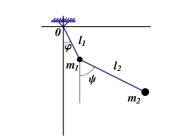
Figure 1: Two-link pendulum.

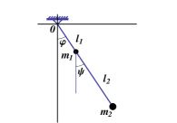
Figure 2: Two-link pendulum in the time moment $T_{1}.$

Namely, let a pendulum have two links of mass $m_{1},$ $m_{2}$ and of lengths $l_{1},$ $l_{2}$ respectively. Then the state of the pendulum is described by angles $\varphi,$ $\psi$ and angle velocities $\dot{\varphi},$ $\dot{\psi}$ ($\varphi$ is the angle between the first bar and the vertical axis; $\psi$ is the angle between the second bar and the vertical axis). Let $F_{1},$ $F_{2}$ be forces applied to the first and the second link respectively. Let $g$ be the acceleration of the free fall. We consider the model of the pendulum with $F_{1}=\alpha u^{3},$ $F_{2}=u,$ where $u$ is a control, $\alpha\in(0,(4/27)l_{1}^{2}/g^{2}].$ Suppose the initial state of the pendulum $(\varphi_{0},\psi_{0},\dot{\varphi}_{0},\dot{\psi}_{0})$ is given. We construct a control $u=u(\varphi,\psi,\dot{\varphi},\dot{\psi},t)$ which calms the vibrations of the pendulum, that is transfers the initial state $(\varphi_{0},\psi_{0},\dot{\varphi}_{0},\dot{\psi}_{0})$ to the origin in some finite time $T,$ i.e. $\varphi(T)=0,$ $\psi(T)=0,$ $\dot{\varphi}(T)=0,$ $\dot{\psi}(T)=0.$

The control motion of the two-link pendulum is described by the equations

$$\begin{array}[]{l}\displaystyle\ddot{\varphi}=-\frac{gm_{1}\sin\varphi+m_{2}\sin(\varphi{-}\psi)\left(g\cos\psi+l_{1}\dot{\varphi}^{2}\cos(\varphi{-}\psi)+l_{2}\dot{\psi}^{2}\right)}{l_{1}\left(m_{1}+m_{2}\sin^{2}(\varphi{-}\psi)\right)}+\alpha u^{3},\\[5.0pt] \displaystyle\ddot{\psi}=\frac{\sin(\varphi{-}\psi)\left((m_{1}+m_{2})\left(g\cos\varphi+l_{1}\dot{\varphi}^{2}\right)+m_{2}l_{2}\dot{\psi}^{2}\cos(\varphi{-}\psi)\right)}{l_{2}\left(m_{1}{+}m_{2}\sin^{2}(\varphi{-}\psi)\right)}+u.\end{array}$$ (34)

Put $x_{1}=\varphi,$ $x_{2}=\dot{\varphi},$ $x_{3}=\psi,$ $x_{4}=\dot{\psi},$ then we obtain the system

$$\dot{x}_{1}=x_{2},\quad\dot{x}_{2}=\beta_{1}(x,u),\quad\dot{x}_{3}=x_{4},\quad\dot{x}_{4}=\beta_{2}(x,u),$$ (35)

where

$$\begin{array}[]{l}\displaystyle\beta_{1}(x,u)=-\frac{gm_{1}\sin x_{1}{+}m_{2}\sin(x_{1}{-}x_{3})\left(g\cos x_{3}{+}l_{1}x_{2}^{2}\cos(x_{1}{-}x_{3}){+}l_{2}x_{4}^{2})\right)}{l_{1}\left(m_{1}{+}m_{2}\sin^{2}(x_{1}{-}x_{3})\right)}+\alpha u^{3},\\[3.0pt] \displaystyle\beta_{2}(x,u)=\frac{\sin(x_{1}{-}x_{3})\left((m_{1}{+}m_{2})(g\cos x_{1}{+}l_{1}x_{2}^{2}){+}l_{2}m_{2}x_{4}^{2}\cos(x_{1}{-}x_{3})\right)}{l_{2}\left(m_{1}+m_{2}\sin^{2}(x_{1}{-}x_{3})\right)}+u,\end{array}$$

The system (35) can be rewritten in the form (3) with $a(x)=(x_{2},0,x_{4},0)^{*},$ $a(0)=0,$ $b_{1}(x)=(0,1,0,0)^{*},$ $b_{2}(x)=(0,0,0,1)^{*},$ $m=2.$ The matrix $K(x)$ from (9) has the form

$$K(x)=(b_{1}(x),{\rm ad}_{a}b_{1}(x),b_{2}(x),{\rm ad}_{a}b_{2}(x))=\left(\begin{array}[]{rrrr}0&-1&0&0\\ 1&0&0&0\\ 0&0&0&-1\\ 0&0&1&0\end{array}\right)$$

and ${\rm rang}\,K(x)=4,$ $x\in{\mathbb{R}}^{4},$ hence, $n_{1}=2,$ $n_{2}=2.$ The conditions (10) imply

$$\begin{array}[]{l}\displaystyle\frac{\partial\varphi_{1}(x_{1},x_{2},x_{3})}{\partial x_{2}}=0,\;\frac{\partial\varphi_{1}(x_{1},x_{2},x_{3})}{\partial x_{4}}=0,\;\frac{\partial\varphi_{1}(x_{1},x_{2},x_{3})}{\partial x_{1}}\neq 0,\\ \displaystyle\frac{\partial\varphi_{2}(x_{1},x_{2},x_{3})}{\partial x_{2}}=0,\;\frac{\partial\varphi_{2}(x_{1},x_{2},x_{3})}{\partial x_{4}}=0,\;\frac{\partial\varphi_{2}(x_{1},x_{2},x_{3})}{\partial x_{3}}\neq 0,\end{array}\quad x\in{\mathbb{R}^{4}}.$$

Choose $\varphi_{1}(x_{1},x_{2},x_{3})=x_{1}-x_{2}$ and $\varphi_{2}(x_{1},x_{2},x_{3})=x_{3}.$ Hence, the non-singular change of variables (11) has the form $z_{1}=x_{1}-x_{3},$ $z_{2}=x_{2}-x_{4},$ $z_{3}=x_{3},$ $z_{4}=x_{4}.$ Then (35) is mapped to the system

$$\dot{z}_{1}=z_{2},\quad\dot{z}_{2}=H_{1}(z_{1},z_{2},z_{3},z_{4},u),\quad\dot{z}_{3}=z_{4},\quad\dot{z}_{4}=H_{2}(z_{1},z_{2},z_{3},z_{4},u),$$ (36)

$$\begin{array}[]{l}\displaystyle H_{1}(z,u)=-\frac{1}{l_{1}l_{2}(m_{1}{+}m_{2}\sin^{2}z_{1})}(l_{2}m_{1}g\sin(z_{1}{+}z_{3}){+}l_{2}m_{2}\sin z_{1}(g\cos z_{3}{+}l_{2}z_{4}^{2}{+}\\[5.0pt] \qquad\qquad\quad+l_{1}(z_{2}{+}z_{4}^{2})\cos z_{1}){+}l_{1}\sin z_{1}(l_{2}m_{2}z_{4}^{2}\cos z_{1}{+}(m_{1}{+}m_{2})(g\cos(z_{1}{+}z_{3}){+}\\[3.0pt] \qquad\qquad\quad+l_{1}(z_{2}{+}z_{4})^{2}))){+}\alpha u^{3}{-}u,\\[5.0pt] \displaystyle H_{2}(z,u)=\frac{\sin z_{1}(l_{2}m_{2}z_{4}^{2}\cos z_{1}{+}(m_{1}{+}m_{2})(g\cos(z_{1}+z_{3})+l_{1}(z_{2}{+}z_{4})^{2}))}{l_{2}(m_{1}{+}m_{2}\sin^{2}z_{1})}+u.\end{array}$$

Notice that for a fixed $z$ the function $H_{1}(z,u)$ is a cubic polynomial with respect to $u.$ We choose controls $u_{1}^{+}(z)$ and $u_{1}^{-}(z)$ as solutions of equations $H_{1}(z,u)=\varepsilon_{1}^{+},$ $H_{1}(z,u)=-\varepsilon_{1}^{-}$ respectively (we do not give the explicit formulas for these controls since they are too complicated).

Put $w_{1}(z_{1})=-\sqrt{2\varepsilon_{1}^{+}z_{1}}$ for $z_{1}\geq 0$ and $w_{1}(z_{1})=\sqrt{-2\varepsilon_{1}^{-}z_{1}}$ for $z_{1}<0,$ and define

$$u_{1}(z)=\left\{\begin{array}[]{l}u_{1}^{+}(z_{1},z_{2},z_{3},z_{4})\;\;\mbox{if}\;\;z_{2}<w_{1}(z_{1})\;\;\mbox{or}\;\;z_{2}=w_{1}(z_{1})\;\;\mbox{and}\;\;z_{1}\geq 0,\\ u_{1}^{-}(z_{1},z_{2},z_{3},z_{4})\;\;\mbox{if}\;\;z_{2}>w_{1}(z_{1})\;\;\mbox{or}\;\;z_{2}=w_{1}(z_{1})\;\;\mbox{and}\;\;z_{1}\leq 0.\\[3.0pt] \end{array}\right.$$

If the initial point $z_{0}=(z_{10},z_{20},z_{30},z_{40})^{*}$ satisfies the inequality $z_{20}<w_{1}(z_{10})$ then the control $u_{1}^{+}(z)$ transfers the point $z_{0}$ to the point $z_{T_{11}}=\bigl{(}z_{1T_{11}},z_{2T_{11}},$ $z_{3T_{11}},z_{4T_{11}}\bigr{)}^{*}$ in the time $T_{11}=\bigl{(}-z_{20}{+}\sqrt{(z_{20}^{2}{-}2z_{10}\varepsilon_{1}^{+})\varepsilon_{1}^{-}/(\varepsilon_{1}^{+}{+}\varepsilon_{1}^{-})}\bigr{)}\bigl{/}\varepsilon_{1}^{+}$ and further the control $u_{1}^{-}(z)$ transfers the point $z_{T_{11}}$ to the point $z_{T_{1}}=\left(0,0,z_{3T_{1}},z_{4T_{1}}\right)^{*}$ in the time $T_{12}=\sqrt{\frac{z_{20}^{2}-2z_{10}\varepsilon_{1}^{+}}{\varepsilon_{1}^{-}(\varepsilon_{1}^{+}+\varepsilon_{1}^{-})}}.$ Thus, the control $u_{1}(z)$ transfers the initial point $z_{0}$ to the point $z_{T_{1}}$ in the time $T_{1}=T_{11}+T_{12}=\bigl{(}-z_{20}{+}\sqrt{(z_{20}^{2}-2z_{10}\varepsilon_{1}^{+})(\varepsilon_{1}^{+}+\varepsilon_{1}^{-})/\varepsilon_{1}^{-}}\bigr{)}\bigl{/}\varepsilon_{1}^{+}.$

If the initial point $z_{0}$ satisfies the conditions $z_{20}=w_{1}(z_{10})$ and $z_{10}\geq 0$ then the control $u_{1}^{-}(z)$ transfers the point $z_{0}$ to the point $z_{T_{1}}=\left(0,0,z_{3T_{1}},z_{4T_{1}}\right)^{*}$ in the time $T_{1}=T_{12}.$

Analogously, in the case $z_{20}>w_{1}(z_{10})$ the control $u_{1}^{-}(z)$ transfers $z_{0}$ to the point $z_{T_{11}}$ in the time $T_{11}=\bigl{(}z_{20}+\sqrt{(z_{20}^{2}+2z_{10}\varepsilon_{1}^{-})\varepsilon_{1}^{+}/(\varepsilon_{1}^{+}+\varepsilon_{1}^{-})}\bigr{)}\bigl{/}\varepsilon_{1}^{-}$ and further the control $u_{1}^{+}(z)$ transfers the point $z_{T_{11}}$ to the point $z_{T_{1}}=\left(0,0,z_{3T_{1}},z_{4T_{1}}\right)^{*}$ in the time $T_{12}=\sqrt{\frac{z_{20}^{2}+2z_{10}\varepsilon_{1}^{-}}{\varepsilon_{1}^{+}(\varepsilon_{1}^{+}+\varepsilon_{1}^{-})}}.$ Thus, the control $u_{1}(z)$ transfers the point $z_{0}$ to the point $z_{T_{1}}$ in the time $T_{1}=T_{11}+T_{12}=\bigl{(}z_{20}+\sqrt{(z_{20}^{2}+2z_{10}\varepsilon_{1}^{-})(\varepsilon_{1}^{+}+\varepsilon_{1}^{-})/\varepsilon_{1}^{+}}\bigr{)}\bigl{/}\varepsilon_{1}^{-}.$

Finally, if $z_{20}=w_{1}(z_{10})$ and $z_{10}\leq 0$ then the control $u_{1}^{+}(z)$ transfers the point $z_{0}$ to the point $z_{T_{1}}=\left(0,0,z_{3T_{1}},z_{4T_{1}}\right)^{*}$ in the time $T_{1}=T_{12}.$

Thus, on the first step the control $u_{1}(z)$ transfers the point $z_{0}$ to the point $z_{T_{1}}=\left(0,0,z_{3T_{1}},z_{4T_{1}}\right)^{*}$ along the trajectory of the system (36) in the time $T_{1}.$

On the second step the motion continues in the plane $P=\{(z_{1},z_{2},z_{3},z_{4}):z_{1}=z_{2}=0\}.$ To ensure this, we choose a control as a root of the equation

$$H_{1}(0,0,z_{3},z_{4},u)=\alpha u^{3}-u-\frac{g}{l_{1}}\,\sin z_{3}=0.$$ (37)

Notice that if $\alpha\in(0,(4/27)l_{1}^{2}/g^{2}]$ then this equation has at least one positive root and one negative root for any $z_{3}\in{\mathbb{R}}.$ Put

$$\alpha_{0}(z_{3}){=}\sqrt[3]{\frac{g\sin z_{3}}{2\alpha l_{1}}{+}\frac{1}{\alpha}\sqrt{\frac{g^{2}\sin^{2}z_{3}}{4l_{1}^{2}}{-}\frac{1}{27\alpha}}},\quad\beta_{0}(z_{3}){=}\sqrt[3]{\frac{g\sin z_{3}}{2\alpha l_{1}}{-}\frac{1}{\alpha}\sqrt{\frac{g^{2}\sin^{2}z_{3}}{4l_{1}^{2}}{-}\frac{1}{27\alpha}}}.$$

Choose $u_{2}^{+}(z_{3})$ as the maximal root and $u_{2}^{-}(z_{3})$ as the minimal root of the equation (37), i.e.

$$u_{2}^{+}(z_{3})=\alpha_{0}(z_{3})+\beta_{0}(z_{3}),\quad u_{2}^{-}(z_{3})=\frac{1}{2}\left(-1+i\sqrt{3}\right)\alpha_{0}(z_{3})-\frac{1}{2}\left(1+i\sqrt{3}\right)\beta_{0}(z_{3}).$$

Then for all $z_{3}\in{\mathbb{R}}$ we have

$$0<u_{2}^{+}(-\pi/2)\leq u_{2}^{+}(z_{3})\leq u_{2}^{+}(\pi/2),\quad u_{2}^{-}(-\pi/2)\leq u_{2}^{-}(z_{3})\leq u_{2}^{-}(\pi/2)<0.$$

Since $H_{2}(0,0,z_{3},z_{4},u)=u$ then

$$H_{2}(0,0,z_{3},z_{4},u_{2}^{+}(z_{3}))\geq\varepsilon_{2}^{+},\quad H_{2}(0,0,z_{3},z_{4},u_{2}^{-}(z_{3}))\leq-\varepsilon_{2}^{-},$$

where $\varepsilon_{2}^{+}=u_{2}^{+}(-\pi/2),$ $\varepsilon_{2}^{-}=-u_{2}^{+}(\pi/2).$

Consider the trajectories of the system (36) with the controls $u_{2}^{\pm}(z_{3})$ which go to the origin, i.e. the trajectories of the system

$$\dot{z}_{1}=z_{2},\quad\dot{z}_{2}=0,\quad\dot{z}_{3}=z_{4},\quad\dot{z}_{4}=u_{2}^{\pm}(z_{3}),$$

which go to the origin. They belong to the plane $P$ and, in addition, $z_{4}=w_{2}(z_{3}),$ where $w_{2}(z_{3})=-\sqrt{2\int\limits_{0}^{z_{3}}u^{+}(\zeta)d\zeta}$ if $z_{3}\geq 0$ and $w_{2}(z_{3})=\sqrt{-2\int\limits_{z_{3}}^{0}u^{-}(\zeta)d\zeta}$ if $z_{3}\leq 0.$ Define

$$u_{2}(z_{3},z_{4})=\left\{\begin{array}[]{l}u_{2}^{+}(z_{3})\;\;\mbox{if}\;\;z_{4}<w_{2}(z_{3})\;\;\mbox{or}\;\;z_{4}=w_{2}(z_{3})\;\;\mbox{and}\;\;z_{3}\geq 0,\\ u_{2}^{-}(z_{3})\;\;\mbox{if}\;\;z_{4}>w_{2}(z_{3})\;\;\mbox{or}\;\;z_{4}=w_{2}(z_{3})\;\;\mbox{and}\;\;z_{3}\leq 0.\\[3.0pt] \end{array}\right.$$

Like the first step, this control transfers the point $z_{T_{1}}$ to the origin in some finite time $T_{2}-T_{1}.$

Therefore, returning to the initial variables we have that the control

$$u(\varphi,\dot{\varphi},\psi,\dot{\psi};t)=\left\{\begin{array}[]{ll}u_{1}(\varphi{-}\psi,\dot{\varphi}{-}\dot{\psi},\psi,\dot{\psi}),&0\leq t\leq T_{1},\\ u_{2}(\psi,\dot{\psi}),&T_{1}\leq t\leq T_{2},\\ \end{array}\right.$$

transfers the initial point $(\varphi(0),\dot{\varphi}(0),\psi(0),\dot{\psi}(0))$ to the origin along the trajectory of the system (34) in the finite time $T=T_{2}.$

Let us summarize the results. We have proved that the stoppage problem of a controllable two-link pendulum can be solved in the following way. On the first step the control is chosen so that the angles $\varphi,$ $\psi$ and the angular speeds $\dot{\varphi},$ $\dot{\psi}$ become equal in the finite time moment $T_{1},$ i.e. $\varphi(T_{1})=\psi_{(}T_{1})$ and $\dot{\varphi}(T_{1})=\dot{\psi}(T_{1})$ (see fig. 2). Roughly speaking, the two links of the pendulum form a one-link pendulum of length $l=l_{1}+l_{2}.$ Further damping of vibrations of the two-link pendulum preserves this configuration of the links, i.e. we choose the control so that $\varphi(t)=\psi(t)$ and $\dot{\varphi}(t)=\dot{\psi}(t)$ for $t\in[T_{1},T_{2}]$ until the time moment $T_{2}$ when the stoppage occurs.

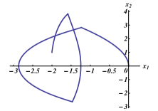
Figure 3: Projection of the phase trajectory of the system (35) on the plane $Ox_{1}x_{2}.$

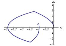
Figure 4: Projection of the phase trajectory of the system (35) on the plane $Ox_{3}x_{4}.$

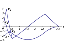
Figure 5: Graphics of components of the trajectory $x(t).$

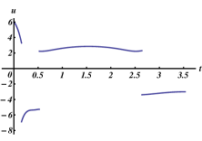
Figure 6: Graphic of control on the trajectory.

As an example, let us transfer the point $x_{0}=(-2,1,-1,0.5)^{*}$ to the origin according to the algorithm described earlier for the system (35) with $m_{1}=m_{2},$ $l_{1}=l_{2}=l,$ $g/l=1,$ $\alpha=1/9$ (see fig. 3–fig. 6). In this case $\varepsilon_{1}^{+}=20,$ $\varepsilon_{1}^{-}=10$ and $T_{11}\approx 0.15814,$ $T_{1}\approx 0.52443,$ $T_{21}\approx 2.64102,$ $T=T_{2}\approx 3.53471.$

7 Classes of staircase systems

In this section we introduce the new classes of nonlinear systems which are mapped on the systems (5). In addition, we give changes of variables satisfying (10)–(11).

7.1

Let the system (3) be of the form

$$\left\{\begin{array}[]{l}\dot{x}_{1}\qquad\;\,=f_{1}(x_{1},\ldots,x_{m{+}1}),\\ \dot{x}_{2}\qquad\;\,=f_{2}(x_{1},\ldots,x_{m{+}2}),\\ .\qquad.\qquad.\qquad.\qquad.\qquad.\\ \dot{x}_{n{-}m}\quad=f_{n{-}m}(x_{1},\ldots,x_{n}),\\ \dot{x}_{n{-}m{+}1}=f_{n{-}m{+}1}(x_{1},\ldots,x_{n},u),\\ .\qquad.\qquad.\qquad.\qquad.\qquad.\\ \dot{x}_{n}\qquad\;\,=f_{n}(x_{1},\ldots,x_{n},u),\end{array}\right.1\leq m<n.$$ (38)

The system (38) for $m=1$ was introduced and considered in the paper [16] and was named the triangular system.

In this subsection we consider the case $m=2$ in detail, i.e. we consider the system

$$\left\{\begin{array}[]{l}\dot{x}_{1}\quad=f_{1}(x_{1},x_{2},x_{3}),\\ \dot{x}_{2}\quad=f_{2}(x_{1},x_{2},x_{3},x_{4}),\\ .\qquad.\qquad.\qquad.\qquad.\qquad.\\ \dot{x}_{n-2}=f_{n-2}(x_{1},x_{2},\ldots,x_{n}),\\ \dot{x}_{n-1}=f_{n-1}(x_{1},x_{2},\ldots,x_{n},u),\\ \dot{x}_{n}\quad=f_{n}(x_{1},x_{2},\ldots,x_{n},u),\qquad\qquad n\geq 3.\\ \end{array}\right.$$ (39)

Here and further $a(x)=(f_{1},\ldots,f_{n-2}),$ $b_{1}=(0,\ldots,0,1,0)^{*},$ $b_{2}=(0,\ldots,0,1)^{*},$ $\beta_{1}(x,u)=f_{n-1}(x_{1},\ldots,x_{n},u),$ $\beta_{2}(x,u)=f_{n}(x_{1},\ldots,x_{n},u).$

Put $\varphi_{1}(x)=x_{1},$ $\varphi_{2}(x)=x_{2}$ and consider the change of variables

$$\left\{\begin{array}[]{l}y_{1}=\varphi_{1}(x)=x_{1}\equiv F_{1}(x_{1}),\quad z_{1}=\varphi_{2}(x)=x_{2}\equiv\Phi_{1}(x_{1},x_{2}),\\ \displaystyle y_{k}=L_{a}^{k-1}\varphi_{1}(x)=\sum\limits_{i=1}^{2k-3}\frac{\partial F_{k-1}(x_{1},\ldots,x_{2k-3})}{\partial x_{i}}\ f_{i}(x_{1},\ldots,x_{i+2})\equiv\\ \quad\;\equiv F_{k}(x_{1},\ldots,x_{2k-1}),\quad 2\leq k\leq p\;\;\mbox{for}\;\;n=2p\;\;\mbox{or}\;\;n=2p-1,\\ \displaystyle z_{k}=L_{a}^{k-1}\varphi_{2}(x)=\sum\limits_{i=1}^{2k-2}\frac{\partial\Phi_{k-1}(x_{1},\ldots,x_{2k-2})}{\partial x_{i}}f_{i}(x_{1},\ldots,x_{i+2})\equiv\\ \quad\;\equiv\Phi_{k}(x_{1},\ldots,x_{2k}),\quad\left\{\begin{array}[]{lcl}2\leq k\leq p&\mbox{if}&n=2p,\\ 2\leq k\leq p-1&\mbox{if}&n=2p-1.\end{array}\right.\end{array}\right.$$ (40)

In addition, if $n=2p$ then put

$$\begin{array}[]{l}F_{p+1}(x,u)=\sum\limits_{i=1}^{n-2}\frac{\partial F_{p}(x_{1},\ldots,x_{n-1})}{\partial x_{i}}f_{i}(x_{1},\ldots,x_{i+2})+\frac{\partial F_{p}(x_{1},\ldots,x_{n-1})}{\partial x_{n-1}}f_{n-1}(x,u),\\[5.0pt] \Phi_{p+1}(x,u)=\sum\limits_{i=1}^{n-2}\frac{\partial\Phi_{p}(x)}{\partial x_{i}}f_{i}(x_{1},\ldots,x_{i+2}){+}\frac{\partial\Phi_{p}(x)}{\partial x_{n-1}}f_{n-1}(x,u){+}\frac{\partial\Phi_{p}(x)}{\partial x_{n}}f_{n}(x,u).\end{array}$$

If $n=2p-1$ then put

$$\begin{array}[]{l}F_{p+1}(x,u)=\sum\limits_{i=1}^{n-2}\frac{\partial F_{p}(x)}{\partial x_{i}}f_{i}(x_{1},\ldots,x_{i+2})+\frac{\partial F_{p}(x)}{\partial x_{n-1}}f_{n-1}(x,u)+\frac{\partial F_{p}(x)}{\partial x_{n}}f_{n}(x,u),\\[5.0pt] \Phi_{p}(x,u)=\sum\limits_{i=1}^{n-2}\frac{\partial\Phi_{p-1}(x_{1},\ldots,x_{n-1})}{\partial x_{i}}f_{i}(x_{1},\ldots,x_{i+2}){+}\frac{\partial\Phi_{p-1}(x_{1},\ldots,x_{n-1})}{\partial x_{n-1}}f_{n-1}(x,u).\end{array}$$

For solvability of the system (40) with respect to $x_{1},$ $\ldots,$ $x_{n}$ we require that $\left|\frac{\partial f_{i}(x_{1},\ldots,x_{i+2})}{\partial x_{i+2}}\right|\geq a>0$ for $i=1,\ldots,n-2.$ Analogously to the paper [16], we prove the equalities

$$\begin{array}[]{l}\displaystyle\frac{\partial F_{k}(x_{1},\ldots,x_{2k-1})}{\partial x_{2k-1}}=\prod\limits_{i=1}^{k-1}\frac{\partial f_{2i-1}(x_{1},\ldots,x_{2i+1})}{\partial x_{2i+1}},\quad k=2,\ldots,p,\\ \displaystyle\frac{\partial\Phi_{k}(x_{1},\ldots,x_{2k})}{\partial x_{2k}}=\prod\limits_{i=1}^{k-1}\frac{\partial f_{2i}(x_{1},\ldots,x_{2i+2})}{\partial x_{2i+2}},\quad k=\left\{\!\!\begin{array}[]{lcl}2,\ldots,p{-}1&\mbox{if}&n=2p{-}1,\\ 2,\ldots,p&\mbox{if}&n=2p.\end{array}\right.\end{array}$$

Hence,

$$\left|\frac{\partial F_{k}(x_{1},\ldots,x_{2k-1})}{\partial x_{2k-1}}\right|\geq a^{k-1}>0,\quad\left|\frac{\partial\Phi_{k}(x_{1},\ldots,x_{2k})}{\partial x_{2k}}\right|\geq a^{k-1}>0.$$

Thus, the change of variables (40) is nonsingular.

Let us explain how to solve the system (40) with respect to $x_{1},$ $\ldots,$ $x_{n}.$ At the beginning we have $x_{1}=y_{1}=h_{1}(y_{1}),$ $x_{2}=z_{1}=h_{2}(z_{1}),$ according to the change of variables. Suppose that for certain $k\geq 2$ the variables $x_{1},$ $\ldots,$ $x_{2k-2}$ are found and have the form

$$\begin{array}[]{l}x_{3}=h_{3}(y_{1},y_{2},z_{1}),\\ x_{4}=h_{4}(y_{1},y_{2},z_{1},z_{2}),\\ .\qquad.\qquad.\qquad.\qquad.\\ x_{2k-3}=h_{2k-3}(y_{1},\ldots,y_{k-1},z_{1},\ldots,z_{k-2}),\\ x_{2k-2}=h_{2k-2}(y_{1},\ldots,y_{k-1},z_{1},\ldots,z_{k-1}).\end{array}$$

Consider the functions $\widehat{F}(x_{2k-1})=F_{k}(x_{1},\ldots,x_{2k-2},x_{2k-1}),$ $\widehat{\Phi}(x_{2k})=\Phi_{k}(x_{1},\ldots,$ $x_{2k-1},x_{2k}).$ The functions $\widehat{F}(x_{2k-1}),$ $\widehat{\Phi}(x_{2k})$ are one-to-one mappings of $\mathbb{R}$ to $\mathbb{R}$. From the equation

$$\begin{array}[]{c}y_{k}=F_{k}(x_{1},\ldots,x_{2k-1})=F_{k}\Bigl{(}h_{1}(y_{1}),h_{2}(z_{1}),\ldots,h_{2k-3}(y_{1},\ldots\\ \ldots,y_{k-1},z_{1},\ldots,z_{k-2}),h_{2k-2}(y_{1},\ldots,y_{k-1},z_{1},\ldots,z_{k-1}),x_{2k-1}\Bigr{)},\end{array}$$

we find $x_{2k-1}=h_{2k-1}(y_{1},\ldots,y_{k},z_{1},\ldots,z_{k-1}).$ Substituting this expression to the equation $z_{k}=\Phi_{k}(h_{1}(y_{1}),h_{2}(z_{1}),\ldots,h_{2k-2}(y_{1},\ldots,y_{k-1},\ldots,z_{1},\ldots,z_{k-1}),x_{2k-1},x_{2k})$ we obtain

$$\begin{array}[]{c}z_{k}=\Phi_{k}(x_{1},\ldots,x_{2k})=\Phi_{k}(h_{1}(y_{1}),h_{2}(z_{1}),\ldots,h_{2k-2}(y_{1},\ldots\\ \ldots,y_{k-1},\ldots,z_{1},\ldots,z_{k-1}),h_{2k-1}(y_{1},\ldots,y_{k},z_{1},\ldots,z_{k-1}),x_{2k}).\end{array}$$

From this equation we find $x_{2k}=h_{2k}(y_{1},\ldots,y_{k},z_{1},\ldots,z_{k}).$

Thus, if $n=2p$ then the nonsingular change of variables (40) maps the system (39) to the system

$$\left\{\begin{array}[]{l}\dot{y}_{i}=y_{i{+}1},\;i=1,\ldots,p{-}1,\;\dot{y}_{p}=F_{p{+}1}\bigl{(}h_{1}(y_{1}),h_{2}(z_{1}),...,h_{2p-1}(y_{1},...,y_{p},\\ \qquad z_{1},...,z_{p-1}),h_{2p}(y_{1},\ldots,y_{p},z_{1},...,z_{p}),u\bigr{)}\equiv H_{1}(y_{1},...,y_{p},z_{1},...,z_{p},u),\\ \dot{z}_{i}=z_{i{+}1},\;i=1,\ldots,p{-}1,\;\dot{z}_{p}=\Phi_{p{+}1}(h_{1}(y_{1}),h_{2}(z_{1}),...,h_{2p-1}(y_{1},...,y_{p},\\ \qquad z_{1},...,z_{p-1}),h_{2p}(y_{1},...,y_{p},z_{1},...,z_{p}),u)\equiv H_{2}(y_{1},...,y_{p},z_{1},...,z_{p},u),\end{array}\right.$$ (41)

and if $n=2p-1$ then one maps the system (39) to the system

$$\left\{\begin{array}[]{l}\dot{y}_{i}=y_{i+1},\quad i=1,\ldots,p-1,\qquad\dot{y}_{p}\quad=H_{1}(y_{1},\ldots,y_{p},z_{1},\ldots,z_{p-1},u),\\ \dot{z}_{i}=z_{i+1},\quad i=1,\ldots,p-2,\qquad\dot{z}_{p-1}=H_{2}(y_{1},\ldots,y_{p},z_{1},\ldots,z_{p-1},u).\end{array}\right.$$ (42)

In the partial case when the first $(n-2)$ equations of the system (39) are linear with respect to the last argument, i.e. the system has the form

$$\left\{\begin{array}[]{lll}\displaystyle\dot{x}_{i}\quad\,=f_{i}(x_{1},\ldots,x_{i+1})+c_{i}x_{i+2},\qquad i=1,\ldots,n{-}2,\\ \dot{x}_{n-1}=f_{n-1}(x_{1},\ldots,x_{n},u),\quad\dot{x}_{n}=f_{n}(x_{1},\ldots,x_{n},u),\\ \end{array}\right.\quad\prod\limits_{i=1}^{n-2}c_{i}\neq 0,$$

the system (40) is solvable with respect to $x_{1},\ldots,x_{n}$ in an obvious way analogously to [14]. For example, the nonsingular change of variables $y_{1}=x_{1},$ $y_{2}=x_{3},$ $z_{1}=x_{2},$ $z_{2}=x_{1}^{2}+x_{4}$ maps the system

$$\dot{x}_{1}=x_{3},\,\dot{x}_{2}=x_{1}^{2}{+}x_{4},\,\dot{x}_{3}=f_{1}(x_{1},x_{2},x_{3},x_{4})\cos u,\,\dot{x}_{4}=f_{2}(x_{1},x_{2},x_{3},x_{4})\sin u{-}2x_{1}x_{3}$$

to the system

$$\dot{y}_{1}=y_{2},\;\dot{y}_{2}=f_{1}(y_{1},z_{1},y_{2},z_{2}-y_{1}^{2})\cos u,\;\dot{z}_{1}=z_{2},\;\dot{z}_{2}=f_{2}(y_{1},z_{1},y_{2},z_{2}-y_{1}^{2})\sin u.$$

7.2

For $n=2p-1\geq 2$ we consider the system

$$\left\{\begin{array}[]{l}\quad\;\dot{x}_{1}\quad\;=f_{1}(x_{1},x_{2},x_{3}),\\ \left\{\begin{array}[]{l}\dot{x}_{2i}\quad=f_{2i}(x_{1},\ldots,x_{2i+3}),\\ \dot{x}_{2i+1}=f_{2i+1}(x_{1},\ldots,x_{2i+3}),\end{array}\right.\quad i=1,\ldots,p-2,\\ \quad\;\dot{x}_{n-1}\,=f_{n-1}(x_{1},\ldots,x_{n},u),\\ \quad\;\dot{x}_{n}\quad\,=f_{n}(x_{1},\ldots,x_{n},u).\end{array}\right.$$ (43)

Put $\varphi_{1}(x_{1},\ldots,x_{n})=x_{1},$ $\varphi_{2}(x_{1},\ldots,x_{n})=x_{2}.$ Then

$$\left\{\!\!\begin{array}[]{l}y_{1}=x_{1}\equiv F_{1}(x_{1}),\\ y_{k}=L_{a}^{k-1}\varphi_{1}=\frac{d}{dt}F_{k-1}(x_{1},\ldots,x_{2k-3})\equiv F_{k}(x_{1},\ldots,x_{2k-1}),\;2\leq k\leq p,\\ z_{1}=x_{2}\equiv\Phi_{1}(x_{1},x_{2}),\\ z_{k}=L_{a}^{k-1}\varphi_{2}=\frac{d}{dt}\Phi_{k-1}(x_{1},\ldots,x_{2k-1})\equiv\Phi_{k}(x_{1},\ldots,x_{2k{+}1}),\;2\leq k\leq p{-}1,\end{array}\right.$$ (44)

and $F_{p+1}(x,u)=\frac{d}{dt}F_{p}(x_{1},\ldots,x_{n}),$ $\Phi_{p}(x,u)=\frac{d}{dt}\Phi_{p-1}(x_{1},\ldots,x_{n}).$ Following the paper [2], suppose that

$$\Delta_{0}=\left|\frac{\partial f_{1}}{\partial x_{3}}\right|\geq\varepsilon_{0},\quad\Delta_{i}=\left|\frac{\partial f_{2i}}{\partial x_{2i+2}}\frac{\partial f_{2i+1}}{\partial x_{2i+3}}-\frac{\partial f_{2i}}{\partial x_{2i+3}}\frac{\partial f_{2i+1}}{\partial x_{2i+2}}\right|\geq\varepsilon_{i},\;i=1,\ldots,p-2.$$

Then the change of variables (44) is nonsingular and maps the system (43) to the system (42).

7.3

For $n=2p$ we consider the system

$$\left\{\begin{array}[]{l}\!\!\!\left\{\begin{array}[]{l}\dot{x}_{2i-1}=f_{2i-1}(x_{1},\ldots,x_{2i+2}),\\ \dot{x}_{2i}\quad=f_{2i}(x_{1},\ldots,x_{2i+2}),\end{array}\right.\quad i=1,\ldots,p-1,\\ \;\;\,\dot{x}_{n-1}\,=f_{n-1}(x_{1},\ldots,x_{n},u),\\ \;\;\,\dot{x}_{n}\quad\,=f_{n}(x_{1},\ldots,x_{n},u).\\ \end{array}\right.$$ (45)

Put $\varphi_{1}(x)=x_{1},$ $\varphi_{2}(x)=x_{2}$ and

$$y_{k}=L_{a}^{k-1}\varphi_{1}(x),\quad z_{k}=L^{k-1}_{a}\varphi_{2}(x),\quad k=1,\ldots,p.$$ (46)

Suppose that

$$\left|\!\displaystyle\frac{\partial f_{2i{-}3}(x_{1},\ldots,x_{2i})}{\partial x_{2i-1}}\displaystyle\frac{\partial f_{2i{-}2}(x_{1},\ldots,x_{2i})}{\partial x_{2i}}-\displaystyle\frac{\partial f_{2i{-}3}(x_{1},\ldots,x_{2i})}{\partial x_{2i}}\displaystyle\frac{\partial f_{2i{-}2}(x_{1},\ldots,x_{2i})}{\partial x_{2i-1}}\!\right|\geq\varepsilon$$

for $i=2,\ldots,p$ and $\varepsilon>0.$ Then the change of variables (46) is nonsingular and maps the system (45) to the system (41).

7.4

For a fixed $k$ such that $8\leq 2k\leq n{+}1$ we consider the system

$$\left\{\begin{array}[]{l}\dot{x}_{i}\quad\,=f_{i}(x_{1},\ldots,x_{k}),\qquad\;\;\;i=1,\ldots,k{-}1,\\ \dot{x}_{i}\quad\,=f_{i}(x_{1},\ldots,x_{i+1}),\qquad i=k,\ldots,n{-}3,\\ \dot{x}_{n-2}=f_{n-2}(x_{1},\ldots,x_{n}),\\ \dot{x}_{n-1}=f_{n-1}(x_{1},\ldots,x_{n},u),\\ \dot{x}_{n}\quad=f_{n}(x_{1},\ldots,x_{n},u).\\ \end{array}\right.$$ (47)

Put $\varphi_{1}(x)=x_{1}$ and $\varphi_{2}(x)=x_{n-k+1}.$ Then the change of variables

$$y_{s}=L^{s-1}_{a}\varphi_{1}(x),\;\;s=2,\ldots,n{-}k{+}1,\quad z_{s}=L^{s-1}_{a}\varphi_{2}(x),\;\;s=2,\ldots,k{-}1,$$

maps the system (47) to the system

$$\left\{\begin{array}[]{lr}\dot{y}_{i}=y_{i+1},\quad i=1,\ldots,n{-}k,&\dot{y}_{n-k+1}=H_{1}(y_{1},\ldots,y_{n-k+1},z_{1},\ldots,z_{k-1},u),\\ \dot{z}_{i}=z_{i+1},\quad i=1,\ldots,k{-}2,&\dot{z}_{k-1}=H_{2}(y_{1},\ldots,y_{n-k+1},z_{1},\ldots,z_{k-1},u).\end{array}\right.$$

References

- [1] A. Krener, On the equivalence of control systems and the linearization of non-linear systems, SIAM J. Control, 11, no. 4 (1973), pp. 670–676.
- [2] S. R. Kou, D. L. Elliot, T. J. Tarn, Observability of nonlinear systems, Inform. Control, 22 (1973), pp. 89–99.
- [3] S. Celikovsky, H. Nijmeijer, Equivalence of nonlinear systems to triangular form: the singular case, Systems and Control Letters, no. 27 (1980), pp. 135–144.
- [4] W. M. Wonham, Linear multivariable control: a geometric approach, Applications of Mathematics, Vol. 10, New York-Heidelberg-Berlin: Springer-Verlag, XV, 1979, 326 pp.
- [5] B. Jakubczyk, W. Respondek, On linearization of control systems, Bull. Acad. Sci. Polonaise Ser. Sci. Math., 28, no. 9–10 (1980), pp. 517–522.
- [6] L. R. Hunt, R. Su, G. Meyer, Design for multi-input nonlinear systems, In: Differential Geometric Control Theory, Burkhauser, New York, 1983, pp. 268–298.
- [7] L. R. Hunt, R. Su, G. Meyer, Global transformations of nonlinear systems, IEEE Trans. on Automatic Control, V. AC-28, no. 1 (1983), pp. 24–31.
- [8] W. Respondek, Geometric methods in linearization of control systems, Banach Center Publ., Semester on Control Theory, 14 (1985), pp. 453–467.
- [9] H. Nijmeijer, On the theory of nonlinear control systems, (English) [A] Three decades of mathematical system theory, Collect. Surv. Occas. 50th Birthday of Jan C. Willems, Lect. Notes Control Inf. Sci. 135 (1989), pp. 339–357.
- [10] S. A. Vakhrameev, Smooth control systems of constant rank and linearizable systems, J. Sov. Math., 55, no. 4 (1991), pp. 1864–1891.
- [11] H. Nijmeijer, A.J. van der Schaft, Nonlinear dynamical control systems, Springer-Verlag, New York, 1990 (4th printing 1998), 467 pp.
- [12] J. Zabczyk, Mathematical control theory: an introduction, Boston-Basel-Berlin: Birkhauser, 1992, 260 pp.
- [13] B. Jakubczyk, W. Respondek, Geometry of feedback and optimal control, CRC Press, 1998, 584 pp.
- [14] E. V. Sklyar, Reduction of triangular controlled systems to linear systems without changing the control, Differ. Equ. 38, no. 1 (2002), pp. 35–46.
- [15] G. M. Sklyar, K. V. Sklyar, S. Yu. Ignatovich, On the extension of the Korobov’s class of linearizable triangular systems by nonlinear control systems of the class , Systems Control Letters, 54 (2005), pp. 1097–1108.
- [16] V.I. Korobov, Controllability and Stability of Certain Nonlinear Systems, Differ. Equ., 9 (1975), pp. 466–469; translation from (Russian) Differ. Uravn., 9, no. 4 (1973), pp. 614–619.
- [17] V. I. Korobov, S. S. Pavlichkov, Global properties of the triangular systems in the singular case, J. Math. Anal. Appl., 342, no. 2 (2008), pp. 1426–1439.
- [18] V. I. Korobov, A general approach to the solution of the problem of synthesizing bounded controls in a control problem Math. USSR Sb., no. 37 (1979), pp. 535–539.
- [19] V. I. Korobov, Method of controllability function, Moskow-Ijevsk: RC Dynamics, 2007, 576 pp.
- [20] V. I. Korobov, G. M. Sklyar, Synthesis of control in equations containing an unbounded operator, (Russian) Teor. Funkts., Funkts. Anal. Priloz., 45 (1986), pp. 45–63.
- [21] V. I. Korobov, G. M. Sklyar, Methods of constructing positional controls and an admissible maximum principle, Differ. Equ., 26, no. 11 (1990), pp. 1422–1431.
- [22] V. I. Korobov and V. O. Skoryk, Synthesis of restricted inertial controls for systems with multivariate control, J. Math. Anal. Appl., 275 (2002), pp. 84–107.
- [23] L.S. Pontryagin, V.G. Boltyanskij, R.V. Gamkrelidze, E.F. Mishchenko, The mathematical theory of optimal processes, New York: Wiley, 1962, 360 pp.
- [24] P. Hartman, Ordinary differential equations, Society for Industrial Mathematics, 2002, 647 pp.
- [25] A. F. Filippov, Differential equations with discontinuous right-hand sides, Ed. by F. M. Arscott. Transl. from the Russian. (English) Mathematics and Its Applications: Soviet Series, 18. Dordrecht etc.: Kluwer Academic Publishers, 1988, 304 pp.
- [26] V.I. Korobov, A geometrical criterion of local controllability of dynamical systems in the presence of constraints on the control, Differ. Equ., 15 (1980), pp. 1136–1142.