Optimization of collective enzyme activity via spatial localization

Abstract

The spatial organization of enzymes often plays a crucial role in the functionality and efficiency of enzymatic pathways. To fully understand the design and operation of enzymatic pathways, it is therefore crucial to understand how the relative arrangement of enzymes affects pathway function. Here we investigate the effect of enzyme localization on the flux of a minimal two-enzyme pathway within a reaction-diffusion model. We consider different reaction kinetics, spatial dimensions, and loss mechanisms for intermediate substrate molecules. Our systematic analysis of the different regimes of this model reveals both universal features and distinct characteristics in the phenomenology of these different systems. In particular, the distribution of the second pathway enzyme that maximizes the reaction flux undergoes a generic transition from co-localization with the first enzyme when the catalytic efficiency of the second enzyme is low, to an extended profile when the catalytic efficiency is high. However, the critical transition point and the shape of the extended optimal profile is significantly affected by specific features of the model. We explain the behavior of these different systems in terms of the underlying stochastic reaction and diffusion processes of single substrate molecules.

I Introduction

The action of enzymes is essential for nearly all processes in living cells. Often these enzymes are organized into large multi-molecular complexes associated with specific functional tasks (Srere, 1987), and this organization can be crucial to the successful operation of the enzymatic system. These “molecular factory” assemblies, in which the product of one enzymatic reaction becomes the substrate for the next, are common in metabolic pathways of both prokaryotes and eukaryotes. Examples include the cellulosome (Bayer et al., 1998), the pyruvate dehydrogenase complex (de Kok et al., 1998) and glycolytic enzymes (Campanella et al., 2005). In some cases, such as the cellulosome (Bayer et al., 1998), enzymes are arranged on an inert scaffold in a specific way. In others, such as tryptophan synthase complexes (Dunn et al., 2008), direct enzyme-enzyme interactions lead to self-assembly into a complex.

Despite the ubiquity of these multi-enzyme complexes, we still lack a deep understanding of the consequences of particular arrangements of enzymes for metabolic pathway operation. Many advantages of co-localization have been proposed (Gaertner, 1978; Ovádi, 1991; Heinrich et al., 1991), particularly via the direct transfer or “channeling” of substrates from one enzyme to another. For example, reducing the transit time of pathway intermediates between enzymes can minimize the loss of unstable intermediates or the interference of competing pathways. Channeling could also potentially enhance the local density of substrates in the vicinity of the enzymes and reduce exposure to toxic intermediates; however, whether or not these effects can actually occur has been disputed (Cornish-Bowden, 1991; Mendes et al., 1992; Cornish-Bowden and Cárdenas, 1993; Mendes et al., 1996). On the other hand, compartmentalization of metabolic enzymes can also increase the flux of biosynthetic pathways Conrado et al. (2007), indicating that the pathway kinetics can be influenced by localization even in the absence of direct channeling. Similar questions about the role of co-localization also arise in the context of protein signaling cascades. For example, there the clustering of enzymes can generate a greater amplification of the signal than distributing enzymes (van Albada and ten Wolde, 2007; Mugler et al., 2012). However, differing functional criteria between signaling scenarios, where discrimination between different inputs is crucial, and metabolic systems, where maintaining a specific flux may be more desirable, mean that these systems are likely subject to different design pressures. More generally, little is known about the effects of the placement of enzymes beyond simple co-localization or clustering scenarios.

Recently there has been a growing focus on the experimental study of colocalized enzymes. Techniques have been developed that allow for the attachment of enzymes to a scaffold (Conrado et al., 2008), which was shown to significantly increase the yield of the mevalonate production pathway (Dueber et al., 2009). The “single-molecule cut-and-paste” technique (Kufer et al., 2008) allows for the positioning of enzymes on a surface with nanometer precision. DNA origami permits the highly-controlled production of three-dimensional structures (Douglas et al., 2009), enabling the quantitative study of the effects of more complex spatial arrangements of enzymes. Over the last few years much progress has been made in engineering of artificial enzymatic pathways on DNA (Niemeyer et al., 2002; Wilner et al., 2009; Idan and Hess, 2013) and RNA assemblies (Delebecque et al., 2011), even in vivo. In particular, a distance-dependence of the activity of a pathway consisting of glucose oxidase (GOx) and the horseradish peroxidase (HRP) was demonstrated (Fu et al., 2012): when the enzymes are brought closer together, the efficiency of the two enzyme complex increases.

Here we study theoretically the impact of enzyme positioning on the flux of pathways. It has been demonstrated previously (Buchner et al., 2013) that in a simple linear reaction-diffusion model, in different parameter regimes co-localization can increase or decrease the pathway flux compared to the uniform distribution of enzymes. In this paper, we extend these results to a range of reaction-diffusion systems. In particular, we consider also nonlinear reactions and different spatial dimensions. We demonstrate that the qualitative features of these diverse models are similar. In general, a transition occurs as a function of the effective reaction rate between regimes in which clustering or distributing enzymes in space generates a higher pathway efficiency. We calculate the optimal enzyme distribution that maximizes the efficiency of the pathway. The universal nature of our results in these diverse systems shows that the observed transitions arise from general properties of reactions and diffusion, and highlights the applicability of the observed behavior to diverse biochemical pathways.

II Model

We consider a simple model reaction pathway consisting of two enzymatic reaction steps. In the first reaction step, an enzyme $E_{1}$ converts a substrate $S$ into an intermediate $I$; subsequently, a second enzyme $E_{2}$ converts $I$ into the final product of the pathway, $P$. We are interested in how the spatial organization of the enzymes affects the efficiency of the pathway $S\overset{E_{1}}{\to}I\overset{E_{2}}{\to}P$ in converting substrate $S$ to product $P$. To this end we assume that the $E_{1}$ enzymes are fixed in position, and examine the impact of the location of the $E_{2}$ enzymes relative to $E_{1}$. In this scenario, $E_{1}$ enzymes act as a source of intermediate $I$, with a total production rate $J_{1}$. In order to additionally include possible undesirable non-specific competition for the intermediate by secondary pathways, or decay in the case that $I$ is unstable, we also allow for the conversion of $I$ into an alternative waste product $Q$. Under the assumption that these processes are independent of the spatial arrangement of $E_{2}$ enzymes, they are simply modeled as a first-order reaction with a constant, position-independent, rate $\sigma$. The density of intermediate $I$, $\rho({\mathbf{r}},t)$ can then be modeled by the reaction-diffusion equation

$$\frac{\partial\rho(\mathbf{r},t)}{\partial t}=D\nabla^{2}\rho(\mathbf{r},t)-\frac{k_{\rm cat}e(\mathbf{r})\rho(\mathbf{r},t)}{K_{M}+\rho(\mathbf{r},t)}-\sigma\rho(\mathbf{r},t),$$ (1)

where $D$ is the diffusion constant of $I$ and $e(\mathbf{r})$ is the (static) density of $E_{2}$ enzymes. The model is illustrated in Fig. 1. In writing Eq. 1 we have assumed that the conversion of $I$ to $P$ by the enzyme $E_{2}$ can be described by standard Michaelis-Menten kinetics with catalytic rate $k_{\rm cat}$ and Michaelis constant $K_{M}$. We implement the production of intermediate by $E_{1}$ enzymes through boundary conditions to Eq. 1. In this work we restrict ourselves to the case of a uniform source at the inner boundary, $-D\nabla\rho(\mathbf{r}_{\rm in})\cdot\mathbf{n}(\mathbf{r}_{\rm in})=J_{1}/A_{\rm in}$, where $\mathbf{n}(\mathbf{r}_{\rm in})$ is the unit vector normal to the boundary and $A_{\rm in}$ is the area of the inner boundary; thus the total influx integrated over the boundary equals the production rate $J_{1}$. For the outer boundary we limit ourselves to reflective ($\nabla\rho(\mathbf{r}_{\rm out})\cdot\mathbf{n}(\mathbf{r}_{\rm out})=0$) or absorbing ($\rho(\mathbf{r}_{\rm out})=0$) boundary conditions. The former could represent the confinement of the intermediate reaction product by the membranes of a cell or organelle, while the latter might describe an intermediate that can easily cross the membrane and be lost to the extracellular environment. We note that our treatment could easily be generalized to mixed boundary conditions representing partial confinement.

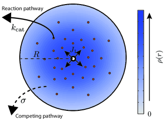
Figure 1: Illustration of the type of reaction-diffusion systems considered in this paper. A cluster of $E_{1}$ enzymes at the center of the system acts as a source of intermediate $I$ with total production rate $J_{1}$. Intermediates diffuse from this center, and can either be converted to the desirable product by the enzymes $E_{2}$ (red circles), via a Michaelis-Menten reaction with catalytic rate $k_{\rm cat}$, or can be lost to a competing pathway with the spatially-uniform rate $\sigma$. We coarse-grain the positions of $E_{2}$ in space into the continuous distribution $e(\mathbf{r})$, and the local density of intermediates as $\rho(\mathbf{r})$. While a two-dimensional system with a hard-wall outer boundary is shown here for clarity, we consider systems of all dimension as well as different outer boundary conditions.

In the following we will be concerned only with the steady-state flux through the reaction pathway. At steady-state form, Eq. 1 can be recast into the dimensionless form

$$0=\nabla^{2}\rho^{\prime}(\mathbf{r^{\prime}})-\frac{\alpha e^{\prime}(\mathbf{r^{\prime}})\rho^{\prime}(\mathbf{r^{\prime}})}{1+\gamma\rho^{\prime}(\mathbf{r^{\prime}})}-\beta\rho^{\prime}(\mathbf{r^{\prime}}),$$ (2)

where $\mathbf{r^{\prime}}$ denotes that the spatial coordinate has been rescaled by a characteristic length-scale of the system, $R$, which we will take to be the system size; and $\rho^{\prime}$ indicates that the density has further been rescaled such that the total production rate of intermediate is equal to $1$. Additionally, we have defined the rescaled enzyme density $e^{\prime}(\mathbf{r})=e(\mathbf{r})/\bar{e}$ with $\bar{e}=V^{-1}\int_{V}e(\mathbf{r}){\rm d}\mathbf{r}$ the average enzyme density over the system volume $V$. The dimensionless parameters $\alpha=(k_{\rm cat}\bar{e}/K_{M})(R^{2}/D)$ and $\beta=\sigma(R^{2}/D)$ respectively capture the relative timescales of reactions with $E_{2}$ and with secondary pathway enzymes, compared to the typical time to diffuse a distance $R$. The parameter $\gamma=J_{1}R^{2-d}/(K_{M}D)$, where $d$ is the spatial dimension, represents the rate of influx of intermediate relative to the level at which $E_{2}$ enzymes become saturated, and includes the effect of varying the activity of $E_{1}$ enzymes via the intermediate production rate $J_{1}$. In the following we drop the prime notation and work exclusively with the dimensionless system; this should not be a source of confusion.

Integrating Eq. 2 and applying the boundary conditions leads to the flux-conservation equation

$$1=\underbrace{\int_{V}\frac{\alpha e(\mathbf{r})\rho(\mathbf{r})}{1+\gamma\rho(\mathbf{r})}{\rm d}\mathbf{r}}_{\displaystyle J_{2}/J_{1}}+\underbrace{\int_{V}\beta\rho(\mathbf{r}){\rm d}\mathbf{r}-\int_{\partial V}\nabla\rho(\mathbf{r})\cdot\mathbf{n}(\mathbf{r}){\rm d}\mathbf{r}}_{\displaystyle J_{\rm loss}/J_{1}}.$$ (3)

On the left hand side we have the (rescaled) production of intermediate by $E_{1}$. This must be balanced by the flux of reactions by $E_{2}$ enzymes, $J_{2}/J_{1}$, plus the loss of intermediate. This loss can occur to secondary pathways (the second term on the right hand side of Eq. 2), and via escape at the boundaries of the system (the third term, where $\partial V$ is the outer boundary of the system that is not a source of intermediate). Assuming that the efficiency of the conversion of substrate to intermediate by $E_{1}$ is independent of the localization of $E_{2}$ enzymes, such that $J_{1}$ is constant, the efficiency of the system can be described by the ratio $J_{2}/J_{1}$, the fraction of intermediates that are converted into the correct product $P$. In this work we will examine how changing $e(\mathbf{r})$ affects the pathway efficiency $J_{2}/J_{1}$. To compare different enzyme profiles on an equal footing, the total amount of $E_{2}$ is held constant via the condition $V^{-1}\int_{V}e(\mathbf{r}){\rm d}\mathbf{r}=1$.

In the remainder of this paper we systematically characterize the effects of varying $E_{2}$ localization in different regimes of Eq. 2. In the section ‘Linear reaction models’ we will focus on the low density limit of the intermediate product, in which the rate of reaction with $E_{2}$ becomes linear in $\rho(\mathbf{r})$. It was previously shown (Buchner et al., 2013) that in an open one-dimensional system where intermediate is lost at an absorbing boundary, different parameter regimes exist in which the optimal enzyme profile consists of either co-localization of $E_{2}$ with $E_{1}$, or a configuration wherein only a fraction of $E_{2}$ enzymes are co-localized and the remainder are distributed over a finite region. Here we extend these results to consider closed systems where the loss of intermediate occurs only via position-independent secondary reactions, and to three- and two-dimensional systems. Finally, in the section ‘Non-linear reactions’ we consider also the full non-linear reaction model. In all cases we observe a transition in the optimal profile from co-localized to distributed as a function of the system parameters, analogous to that reported in the specific minimal model of Buchner et al. (2013), demonstrating the generality of the underlying physics. However, we also highlight qualitative differences in the phenomenology of these different regimes.

III Results

III.1 Linear reaction models

III.1.1 Enzyme exposure

To understand the impact of different enzyme configurations on the overall pathway flux, the concept of integrated “enzyme exposure” has proven to be useful (Buchner et al., 2013). It allows for the decomposition of the reaction flux of linear systems into two factors, one that depends only on the enzyme distribution $e(\mathbf{r})$ and describes the diffusive dynamics of the system, and another that is independent of $e(\mathbf{r})$ but captures the reaction dynamics. The concept is best explained with the help of a thought experiment where we first consider the dynamics of individual intermediate molecules in the absence of any $E_{2}$ enzymes, also shown schematically in Fig. 2. We introduce a single intermediate molecule at $t=0$ at the source, and track its stochastic path until it leaves the system, either through the boundary of the system or via a reaction with a competing pathway. We denote the time at which the trajectory ends, either by escaping at the system boundary or through a competing reaction, as $t_{\rm escape}$. By repeatedly applying this procedure for many such molecules, we can generate an ensemble of trajectories $\mathbf{r}(t)$ through the system that is independent of the distribution of $E_{2}$ enzymes.

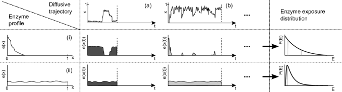
Figure 2: A schematic illustration of the underlying concept of “enzyme exposure”. Diffusion generates an ensemble of trajectories of intermediate molecules (top row), which have different enzyme exposure values in the presence of different enzyme distribution patterns (left column). For example, the diffusive path (a) spends a relatively long time in the vicinity of the origin. This leads to a higher enzyme exposure value $E=\int_{0}^{t_{\rm escape}}e(x(t))dt$ (shaded areas) for an enzyme distribution that is clustered near the origin [distribution (i), middle row]. Trajectory (b), which spends little time near the origin, leads to a very small exposure value in the presence of distribution (i). For a more uniformly distributed profile [distribution (ii), bottom row] the exposure value is determined primarily by how long the particle stays in the system. Enumerating the value of $E$ for all possible diffusive trajectories leads to the $e(x)$-dependent distribution of enzyme exposures $P(E)$ (right column).

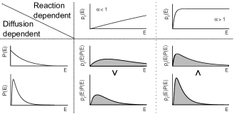
Figure 3: The reaction efficiency can be calculated as the overlap integral of the $e(\mathbf{r})$-dependent enzyme exposure distribution $P(E)$, and the $\alpha$-dependent reaction probability $p_{r}(E)$, according to $J_{2}/J_{1}=\int_{0}^{\infty}P(E)p_{r}(E){\rm d}E$. Broader exposure distributions, which maximize the likelihood of large-$E$ trajectories, are preferable when $\alpha$ is small (middle column). Narrower $P(E)$ distributions, which minimize the likelihood of small values of $E$, are favored when $\alpha$ is large (right).

Next, we suppose that we were to re-introduce $E_{2}$ enzymes according to the distribution $e(\mathbf{r})$. For each of the diffusive intermediate trajectories generated above, the instantaneous propensity of reaction with an $E_{2}$ enzyme is given by $\alpha e(\mathbf{r}(t))$ (in the linear reaction regime). For each trajectory, the survival probability $S(t)$ that no reaction has occurred up to the time $t$ follows the differential equation $\dot{S}(t)=-\alpha e(\mathbf{r}(t))S(t)$. We can therefore straightforwardly calculate the probability that a reaction would have occurred at some point along the trajectory as $1-\exp\left[-\alpha\int_{0}^{t_{\rm escape}}e(\mathbf{r}(t)){\rm d}t\right]$.

Finally, we define the enzyme exposure for each individual trajectory to be

$$E=\int_{0}^{t_{\rm escape}}e(\mathbf{r}(t)){\rm d}t.$$ (4)

The ensemble of possible trajectories in the system $\mathbf{r}(t)$, each with a characteristic $t_{\rm escape}$, therefore generates a distribution of enzyme exposure values, $P(E)$. This distribution is a function of the arrangement of $E_{2}$ enzymes $e(\mathbf{r})$ via Eq. 4, but importantly is independent of the reaction with $E_{2}$ enzymes, since the diffusive trajectories were generated in the absence of such reactions. The probability of reaction along a trajectory is then given by $p_{r}(E)=1-\exp[-\alpha E]$, which depends on the reaction parameter $\alpha$ but crucially not on the $E_{2}$ distribution itself. The overall probability of reaction is recovered by the expression

$$\frac{J_{2}}{J_{1}}=\int_{0}^{\infty}P(E)p_{r}(E){\rm d}E,$$ (5)

which ensures a proper weighting of the likelihood of a particular trajectory occurring (see the Supplementary Material SI for a derivation showing the equivalence of Eq. 5 with the expression for $J_{2}/J_{1}$ defined in Eq. 3). Thus, as depicted schematically in Fig. 3, we have decomposed the reaction-diffusion dynamics of Eq. 2 into a diffusion- and $e(\mathbf{r})$-dependent component $P(E)$, and a reaction-dependent component $p_{r}(E)$, with the efficiency of the reaction pathway determined by the product of these two distributions.

Interestingly, using Eq. 3 the reaction efficiency can be rewritten as

$$\frac{J_{2}}{J_{1}}=1-\int_{0}^{\infty}P(E)e^{-\alpha E}{\rm d}E=1-\frac{J_{\rm loss}}{J_{1}},$$ (6)

wherein we see that the fraction of intermediate molecules lost via the reaction $I\to Q$ or through the boundary, $J_{\rm loss}/J_{1}$, takes the form of the Laplace transform of $P(E)$, with transform variable $\alpha$. It is generally more straightforward to calculate $J_{\rm loss}$ as a function of $\alpha$ for a given $E_{2}$ profile $e(\mathbf{r})$ and to compute $P(E)$ by performing an inverse Laplace transformation, than it is to calculate $P(E)$ directly from considering individual diffusive trajectories.

III.1.2 A competing pathway

We now consider the case where intermediates are unable to cross a cell membrane and therefore cannot escape via the boundaries of the system, but can be lost to a competing, spatially-uniform, reaction pathway. That is, all intermediate molecules ultimately end up as either the desirable product $P$ or undesirable product $Q$. For a one-dimensional system in the linear, low-density, regime of the Michaelis-Menten reaction, we have the reaction-diffusion equation

$$0=\partial^{2}_{x}\rho(x)-\alpha e(x)\rho(x)-\beta\rho(x)\;$$ (7)

with a source boundary condition at the left edge, $\partial_{x}\rho|_{x=0}=-1$, and a reflecting boundary at the right edge, $\partial_{x}\rho|_{x=1}=0$. The parameters $\alpha$ and $\beta$, defined above, reflect the relative reactivities of intermediate with $E_{2}$ and competing pathway enzymes respectively, in units of the typical time to diffuse a distance of the system size $R$. Consequently, $\alpha$ and $\beta$ can also be interpreted as describing the system size in units of the typical distance from the source at $x=0$ that an intermediate molecule will diffuse before leaving the system via reaction with $E_{2}$ and via the competing pathway, respectively. When $\beta\ll 1$, intermediate molecules will typically be able to explore the entire system, and therefore we should expect that the spatial arrangement of enzymes will have little effect on the reaction flux, since the intermediate will be exposed to each enzyme regardless of where it is placed. In contrast, when $\beta\gg 1$ very few intermediate molecules will diffuse far from the source and we should expect that the amount of enzyme located close to the source will have a strong influence on the pathway efficiency.

We begin by examining the case where $E_{2}$ enzymes have the uniform density $e_{\rm u}(x)=1$ throughout the domain $x\in[0,1]$. Substituting into Eq. 7 leads to the straightforward solution $\rho_{\rm u}(x)=\cosh\left[(1-x)\sqrt{\alpha+\beta}\right]/(\sqrt{\alpha+\beta}\sinh\sqrt{\alpha+\beta})$. From this expression the reaction efficiency can be calculated using the definitions in Eq.3, and is given by

$$\left(\frac{J_{2}}{J_{1}}\right)_{\rm u}=\frac{\alpha}{\alpha+\beta}.$$ (8)

Next we suppose that all $E_{2}$ enzymes are clustered at $x=0$, co-localized with $E_{1}$. This is represented by the distribution $e_{\rm c}(x)=\delta(x)$, which leads to the solution $\rho_{\rm c}(x)=\rho_{0}\cosh\left[(1-x)\sqrt{\beta}\right]/\cosh\sqrt{\beta}$, where $\rho_{0}$ can be found by imposing the flux conservation equation (3) with $\gamma=0$. Ultimately, this leads to a reaction efficiency of

$$\left(\frac{J_{2}}{J_{1}}\right)_{\rm c}=\frac{\alpha}{\alpha+\beta^{1/2}\tanh\beta^{1/2}}.$$ (9)

Comparing these two expressions, we can see that for given values of $\alpha$ and $\beta$ the clustered $E_{2}$ configuration always generates a higher reaction flux than a uniform distribution of $E_{2}$ since $\tanh\beta^{1/2}\leq\beta^{1/2}$. (Note that this situation changes considerably if we allow for escape of intermediate at the boundary in addition to loss via secondary reactions. For full details, see Appendix.) Intuitively, this is because secondary reactions, parametrized by $\beta$, limit how far intermediate molecules diffuse away from the source at $x=0$. Thus for a uniform profile, the effective enzyme density that intermediate molecules will experience is reduced; for large $\beta$, this reduction is by a factor of order $\beta^{1/2}$. This effect can also be quantified by studying the enzyme exposure distributions corresponding to the two enzyme profiles, which are SI

$$P_{\rm u}(E) =\beta e^{-E\beta},$$ (10a)

$$P_{\rm c}(E) =\beta^{1/2}\tanh\beta^{1/2}e^{-E\beta^{1/2}\tanh\beta^{1/2}}.$$ (10b)

We see that $P_{\rm u}(E)$ is more concentrated near $E=0$ than $P_{\rm c}(E)$; thus a higher proportion of trajectories rapidly react via secondary pathways before being exposed to a significant level of $E_{2}$ enzyme. These intermediate molecules therefore have a low probability of reacting with $E_{2}$ leading to a low pathway efficiency.

We now turn to the question of what is the $E_{2}$ profile that maximizes the reaction efficiency. We investigated this by performing a numerical optimization of $e(x)$ on a discrete lattice of $N$ sites, as described previously (Buchner et al., 2013). Briefly, we use an evolutionary algorithm with mutation and mixing. We begin each optimization step with a trial enzyme profile $e(x)$. We generate 50 mutations of this profile, by selecting one lattice site at random and moving a random fraction of the $E_{2}$ enzymes at this site to another randomly-chosen site. For each of these modified $e(x)$ profiles, the discrete reaction-diffusion system (an order-$N$ linear system) is solved and $J_{2}/J_{1}$ calculated. As the initial profile for the next mutation round, we take the mean of the ten most-efficient mutant configurations in the previous round. We have found this procedure to achieve more rapid and robust convergence than a simple Monte Carlo exploration of the space of possible configurations. The optimal profiles reported below are the configurations with the highest reaction efficiency that occurred at any point during the optimization process.

The upper panels of Fig. 4 show the optimal enzyme profiles found numerically for different combinations of the parameters $\alpha$ and $\beta$. Importantly, we find that the fully clustered configuration is not always the optimal distribution; for different parameter values, the optimal $E_{2}$ profile can be either a fully-clustered configuration at $x=0$, or a mixed profile in which only a finite fraction of the available enzymes are clustered. This is reminiscent of the behavior of an open system with an absorbing boundary but without a competing pathway, reported previously (Buchner et al., 2013), although the shape of the enzyme profile differs.

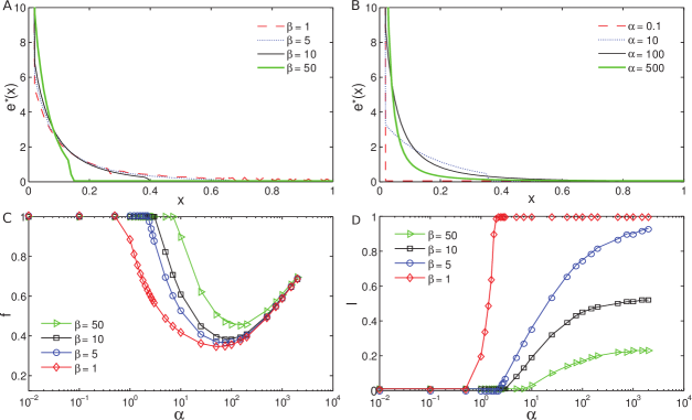
Figure 4: (Top) Optimal $E_{2}$ enzyme profiles as (A) $\beta$ is varied at constant $\alpha=50$, and (B) $\alpha$ is varied at constant $\beta=5$. All the optimal profiles are obtained by numerical optimization on a lattice with $N=100$ sites. (Bottom) Quantifying the optimal profile. (C) The fraction $f$ of $E_{2}$ enzymes that are clustered in the optimal profile shows a non-monotonic dependence on $\alpha$. (D) The extent of distributed enzymes $l$ increases monotonically with $\alpha$ until reaching a maximal extension that depends on $\beta$.

We quantify the level of clustering in the optimal enzyme profiles (see Fig. 4, lower panels) by the fraction $f$ of $E_{2}$ that are located at the lattice site $x=0$, and the extent of the optimal profile via the distance $l$ over which the optimal enzyme density is above a threshold of $10^{-3}$. Examining first the behavior as $\beta$ is varied (upper left) we see that for larger $\beta$ the enzyme profile becomes more concentrated at smaller values of $x$; $f$ increases and $l$ decreases. This is simply because intermediate molecules typically diffuse less far from the source before reacting via the secondary pathway. Turning now to the behavior as a function of $\alpha$, we see that there exists a sharp transition: below a ($\beta$-dependent) critical value of $\alpha$, the optimal profile is the fully-clustered configuration, $f=1$. As the threshold is crossed, a fraction of enzymes are relocated away from $x=0$ and distributed over an extended region; $f$ decreases and $l$ increases. Interestingly, as $\alpha$ is increased further we find that the available enzymes tend to once again relocate towards $x=0$; $f$ passes though a minimum and begins to increase again. This is not accompanied by a decrease in $l$, but the density of enzymes is reduced at larger $x$ and increased at smaller $x$. For large $\alpha\gtrsim 1000$, the optimal profiles for different values of $\beta$ become more similar (with the exception of the position at which the enzyme profile cuts off sharply, which remains $\beta$-dependent).

The pattern of changes in the optimal profile can be understood as follows. When $\alpha$ is small the reaction efficiency is optimized by a clustered configuration since this is the enzyme distribution that maximizes the number of large-$E$ trajectories. However, the clustered configuration also leads to a large population of trajectories, those corresponding to $I$ molecules that rapidly diffuse away from the cluster and do not return, with extremely small values of $E$. At intermediate values of $\alpha$, it becomes favorable to move some enzymes away from the cluster and to distribute more widely. This increases the probability of reaction for trajectories that rapidly leave the cluster, while not significantly reducing the probability of reaction for trajectories that spend a significant amount of time in the vicinity of the cluster. For large $\alpha$, however, the need for these distributed enzymes is reduced, since only for those trajectories that rapidly escape via the secondary pathway is the reaction probability much less than 1. Thus, by again concentrating enzymes around $x=0$ it is possible to maximize the probability of reaction for those trajectories that spend only a very short time in the system, and therefore do not diffuse far from $x=0$. Here we see a significant difference from an open system where loss occurs only at the boundary, for which there is no impetus to cluster enzymes again (Buchner et al., 2013). If loss occurs only at $x=1$, intermediate molecules must always diffuse past all $E_{2}$ molecules in order to escape from the system. However, if loss occurs in the vicinity of $x=0$, then $E_{2}$ enzymes placed far from the source are essentially wasted.

III.1.3 Higher-dimensional systems

We now consider systems in more than one spatial dimension, beginning with a three-dimensional spherical geometry. We impose angular symmetry, such that position within the system can be parametrized by a single radial coordinate, $r$. We place $E_{1}$ enzymes at the center $r=0$ of a spherical volume of radius $1$. In the first instance, we neglect any secondary pathways ($\beta=0$) and impose an absorbing boundary condition at $r=1$. With these simplifications, Eq. 2 becomes

$$0=r^{-2}\partial_{r}\left[r^{2}\partial_{r}\rho(r)\right]-\alpha e(r)\rho(r)$$ (11)

with the boundary conditions $[4\pi r^{2}\partial_{r}\rho(r)]_{r=0}=-1$, accounting for the production of intermediate, and $\rho(1)=0$. This system is a three-dimensional analog of that discussed previously in (Buchner et al., 2013).

We once again begin by exploring the configurations in which $E_{2}$ are either placed on a shell of radius $r_{0}$, $e_{\rm c}(r)=\delta(r-r_{0})/(3r_{0}^{2})$, or uniformly distributed throughout the spherical volume, $e_{\rm u}(r)=1$ (recall that these distributions are scaled by the average density such that $V^{-1}\int_{V}e(\mathbf{r}){\rm d}\mathbf{r}=1$). The reaction efficiency is then given by

$$\left(\frac{J_{2}}{J_{1}}\right)_{\rm c}=\frac{\frac{\alpha}{3}(1-r_{0})}{r_{0}+\frac{\alpha}{3}(1-r_{0})}$$ (12)

for the enzyme shell, and

$$\left(\frac{J_{2}}{J_{1}}\right)_{\rm u}=1-\sqrt{\alpha}\ {\rm csch}\sqrt{\alpha}.$$ (13)

for uniformly distributed enzymes.

As the shell radius $r_{0}$ approaches zero, the efficiency of reaction of intermediate with $E_{2}$ approaches one. However, this situation is not physically realistic, as enzymes have a finite size and there will be a maximum packing density which limits the potential shell radii. If $r_{0}$ is taken to be small but finite, for small $\alpha$ the clustering of enzymes into a tightly-packed shell configuration still achieves a higher reaction flux (see Fig. 5A) than the uniformly-distributed configuration. However above a critical ($r_{0}$-dependent) $\alpha$ value, the uniform enzyme arrangement is able to achieve a higher reaction flux. This transition is analogous to that seen in the equivalent one-dimensional system (Buchner et al., 2013). However, as can be seen in Fig. 5A the region in which the uniform enzyme distribution is favored is shifted to much higher $\alpha$ values, from $\alpha\approx 9$ in the one-dimensional system up to $\alpha\approx 85$ for the three-dimensional system with $r_{0}=0.05$. Since the transition occurs at extremely large $\alpha$ values, for which almost all intermediate particles react, the difference between the efficiencies of the two profiles is extremely small. Furthermore, in the low-$\alpha$ domain the advantage provided by clustering of enzymes is much more significant than in the one-dimension system, with an increase in the reaction flux by more than a factor of four. Thus clustering of enzymes is more strongly favored in three-dimensional than in one-dimensional systems.

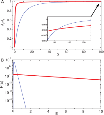
Figure 5: (A) Comparison of the reaction flux for clustered (thick red line, $r_{0}=0.05$) and distributed (thin blue line) $E_{2}$ profiles. The clustered distribution achieves a significantly higher efficiency for small $\alpha$. A transition is observed at $\alpha\approx 85$, above which the distributed profile reaches a marginally higher efficiency. (B) Enzyme exposure distributions for the clustered (thick red, $r_{0}=0.05$) and the distributed (thin blue) $E_{2}$ profiles. The enzyme exposure distribution for the distributed $E_{2}$ profile is sharply peaked at $E\ll 1$, whereas the distribution for the clustered profile extends to large values of $E$.

Calculating the corresponding enzyme exposure distributions,

$$P_{\rm u}(E) =2\sum_{n=1}^{\infty}(-1)^{n+1}(\pi n)^{2}e^{-(\pi n)^{2}E},$$ (14a)

$$P_{\rm c}(E) =\frac{3r_{0}}{1-r_{0}}e^{-\frac{3r_{0}}{1-r_{0}}E},$$ (14b)

we find that $P_{\rm u}(E)$ is sharply peaked around a small but finite value of $E$ (see Fig. 5B; the mean and variance of $P_{\rm u}(E)$ are $1/6$ and $1/90$, respectively). For the clustered profile, $P_{\rm c}(E)$ takes its customary exponential form. Thus we can see that for small $\alpha\ll 1$, almost all of the weight of $P_{\rm u}(E)$ lies in the region $E\lesssim 1$ where $p_{r}(E)$ is small; the exponential tail of $P_{\rm c}$, though, results in a larger mean value of $E$ and more trajectories in regions where $p_{r}(E)$ is significant. Thus for $\alpha\ll 1$, the clustered configuration is more efficient. On the other hand when $\alpha\gg 1$, essentially all the probability weight of $P_{\rm u}(E)$ lies in the region $E\gtrsim\alpha^{-1}$, where $p_{r}(E)\approx 1$; however, $P_{\rm c}(E)$ is actually largest in the region $E\ll 1$ where $p_{r}(E)$ is small. These trajectories, which correspond to $I$ molecules that rapidly diffuse away from the $E_{2}$ cluster and do not return, generally will not lead to reactions and thus reduce the relative efficiency of the clustered configuration.

How can the greater impact of clustering in a spherical geometry be understood intuitively? On a typical path to the boundary, a single intermediate particle originated form the center explores only a fraction of the whole sphere. If the same number of enzymes are distributed on a spherical shell further from the center, the effective “reaction cross-section” is smaller because the fraction of this shell that an intermediate will typically explore decreases, and with it the fraction of the enzymes in the system to which the intermediate molecule will be exposed. This is in contrast to the one-dimensional case, where the particle passes all enzymes before getting absorbed by the boundary. To derive a benefit from distributing enzymes, a larger $\alpha$ value is therefore required in three dimensions to compensate for this reduction in the effective level of $E_{2}$ enzymes to which intermediate molecules are exposed.

Next we investigated the optimal enzyme distribution as a function of the control parameter $\alpha$. As noted above, if the clustering of all $E_{2}$ enzymes at $r=0$ is permitted then $J_{2}/J_{1}\to 1$ independent of $\alpha$, yielding the maximal possible flux. However, we note again that this configuration with an infinite packing density is not physically realizable. Instead we impose a limit to the possible packing density through a minimal radius $r_{0}$ within which $E_{2}$ enzymes cannot be placed. We adapt the optimization procedure described above by solving Eq. 11 on a radial lattice where each lattice site represents a concentric shell of the system. This fixes a minimal value of $r_{0,{\rm min}}=(2N)^{-1}$ at the mid-point of the innermost shell; larger values of $r_{0}$ can be prescribed, but not smaller shells.

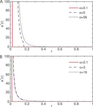
Figure 6: Changes in the optimal enzyme profile as a function of $\alpha$ are qualitatively similar in two and three dimensions. (A) For the three-dimensional system described by Eq. 11, an extended region of distributed enzymes emerges for $\alpha\gtrsim 0.05$. (B) In two dimensions, the critical value for the emergence of a distributed enzyme fraction is $\alpha\approx 0.5$.

As shown in Fig. 6A, when a finite minimal clustering radius is imposed we again find that a purely clustered configuration is optimal for small $\alpha$ while for $\alpha$ larger than a critical value an extended region of distributed enzymes emerges, in the same way as in one dimension Buchner et al. (2013). The critical $\alpha$ value at which this transition occurs is strongly dependent on the minimal allowed radius, $r_{0}$. Interestingly, for $N=100$ and $r_{0}=r_{0,{\rm min}}=0.005$ the transition point $\alpha\approx 0.05$ is significantly lower than in the one-dimensional system, despite the above arguments that distributing enzymes is less efficient in three dimensions than in one; only at $r_{0}\sim 0.2$ does the transition point reach the $\alpha=1$ observed in one dimension. The increased penalty, via the reduction in reaction cross-section, of moving enzymes to larger values of $r$ is instead reflected in the shape of the extended enzyme “tail”: unlike in one dimension, the enzyme density in the extended region of the profile is not constant but decreases roughly as $e^{*}(r)\sim r^{-4}$.

We have seen that one- and three-dimensional systems have qualitatively similar phenomenology in terms of whether a clustered or uniform profile is preferable and in terms of the optimal enzyme profile, although the quantitative aspects of these transitions vary. The same also holds true for the two-dimensional case: we find that this system also displays a transition from a clustered to uniform $E_{2}$ configuration being preferable at an $\alpha$ value between those at which the transition occurs in one- and three-dimensional systems (data not shown). Figure 6B shows that once again an extended optimal profile appears at $\alpha\approx 0.5$ (for $r_{0}=0.005$; the effect of varying $r_{0}$ is much weaker in two dimensions than in three). In the extended region, the optimal density is found to decrease as $e^{*}(r)\sim r^{-2}$. We can therefore see that the underlying physics of these transitions is generic, and is not dependent on the statistics of diffusion in particular dimensions.

III.2 Non-linear reactions

We now turn to the case of fully non-linear reactions. We begin by considering the case $\beta=0$, in which there is no competition with secondary pathways for the intermediate $I$. We furthermore restrict ourselves to a one-dimensional system on the domain $x\in[0,1]$, with $E_{1}$ enzymes located at $x=0$ and an absorbing boundary condition at $x=1$. That is, we consider a reaction-diffusion equation of the form

$$0=\partial_{x}^{2}\rho(x)-\frac{\alpha e(x)\rho(x)}{1+\gamma\rho(x)},$$ (15)

together with source-sink boundary conditions $\partial_{x}\rho|_{x=0}=-1$ and $\rho(1)=0$, where $\gamma$ is the effective saturation parameter defined in the ‘Model’ Section.

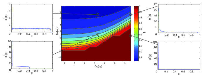
Figure 7: Central panel: the fraction $f$ of $E_{2}$ enzymes that are clustered in the numerically-optimized enzyme distribution (on a lattice of 100 sites) as the parameters $\alpha$ and $\gamma$ are varied. Outer panels depict the optimal profiles at specific parameter combinations, showing how the profile shape changes across the transition from clustered to fully-distributed. Optimizations were run for $2\times 10^{5}$ steps on a lattice of $N=100$ sites, with a solution error-tolerance of $10^{-7}$.

We again seek to find the $E_{2}$ distribution $e(x)$ that maximizes the reaction efficiency $J_{2}/J_{1}$ via numerical optimization. The non-linear nature of the reaction terms mean that the discretized reaction-diffusion equation for a given $e(x)$ no longer takes the form of a linear system that can be solved directly. Instead, we used a shooting approach to calculate $\rho(x)$ and thereby $J_{2}$. An initial trial solution for $\tilde{\rho}(x_{N})$ at the right-most lattice site is selected. This trial is then used to successively solve the non-linear reaction-diffusion equation at the remaining lattice sites (the equation for site $N$ depends on $\rho(x_{N})$ and $\rho(x_{N-1})$, that for site $N-1$ depends on $\rho(x_{N})$, $\rho(x_{N-1})$ and $\rho(x_{N-2})$, and so on). Once a trial solution $\tilde{\rho}(x)$ has been calculated for all sites, this is tested against the reaction-diffusion equation at site $x_{1}$, which includes the source boundary condition. If the equation is satisfied to within a certain tolerance, then the solution is accepted. Otherwise, the trial value of $\tilde{\rho}(x_{N})$ is refined, and the process repeated. The mutation, selection and mixing steps of the optimization were unchanged.

Figure 7 shows results for the optimal enzyme profiles for different values of $\alpha$ and $\gamma$. We first verified that this solution technique accurately reproduces the results of the linear system in the limit of small $\gamma$, which should correspond the results for the linear-reaction case that have been described previously (Buchner et al., 2013). Indeed, we find that when $\alpha<1$ all $E_{2}$ enzymes should be co-localized with the $E_{1}$ enzymes at $x=0$. As $\alpha>1$ is increased, the fraction $f$ of $E_{2}$ enzymes that cluster at $x=0$ decreases with the remaining enzymes being distributed uniformly over an extended region such that $e(x)=1$ in this region. Figure 7 shows that the same qualitative behavior is also observed for larger values of $\gamma$. For all values of $\gamma$ tested, the optimal profile undergoes a transition from fully clustered at small $\alpha$ to a mixed profile with a clustered fraction and extended, lower-density, region for larger $\alpha$. The critical $\alpha$ value at which this transition occurs increases with $\gamma$, since in the fully clustered configuration a larger $\gamma$ serves to reduce the effective reaction rate. Additionally, we find that the optimal profiles deviate in shape and extension away from the source. In the mixed-profile regime, the extended “tail” of enzymes need not have a constant density. This reflects the fact that for intermediate values of $\alpha$ the level of saturation of $E_{2}$ enzymes will vary with position. Finally, it appears that once the transition to a mixed profile has begun, the fraction of $E_{2}$ enzymes clustered at $x=0$ decreases more quickly as $\alpha$ is increased if $\gamma$ is large than if $\gamma$ is small. We attribute this to the fact that large values of $\alpha$ tend to dramatically reduce the intermediate density within the system, thereby moving a system that was in the saturated regime for small $\alpha$ into the unsaturated regime for large $\alpha$. Indeed, for extremely large values of $\alpha$ the optimal profile becomes independent of $\gamma$ and approaches that expected in the linear reaction case.

The inclusion of non-linear reaction terms complicates the analysis of systems of this type via enzyme exposure. This is because the probability of reaction of an individual $I$ molecule depends not only on the enzyme density, but also on other intermediate molecules in the system. One can define the effective enzyme activity at each position as $e(x)/\left[1+\gamma\rho(x)\right]$, and thereby calculate an effective enzyme exposure for a trajectory as $\tilde{E}=\int_{0}^{t_{\rm escape}}e(x(t))/\left[1+\gamma\rho(x(t))\right]{\rm d}t$ taking $\rho(x)$ to be the solution to Eq. 15. However, it must be noted that this does not lead to a true decomposition of the reaction flux into diffusion- and reaction-dependent terms because $\rho(x)$ itself depends on the reaction parameter $\alpha$.

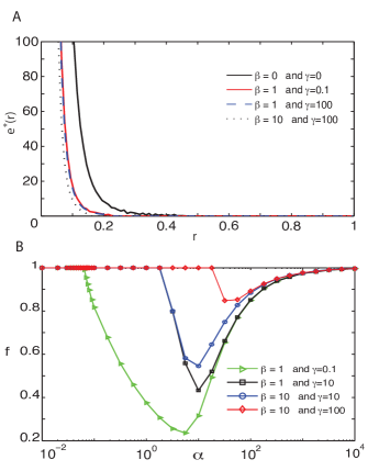
Figure 8: (A) Optimal enzyme distributions for the full model, with parameter values as indicated, with $\alpha=56$. (B) Clustered fraction of $E_{2}$ enzymes in the optimal profile $f$, as a function of the catalytic activity of $E_{2}$. A non-monotonic dependence is seen when $\beta\neq 0$.

Finally, we briefly consider the results of the full model described in Section II, including both a non-linear reaction, $\gamma\neq 0$, and a competing pathway, $\beta\neq 0$, in a radially-symmetric three-dimensional geometry. Figure 8A shows that the optimal enzyme distributions are qualitatively similar to those in Fig. 6A for a system without competition and with only linear reactions. However, examining the fraction of enzymes that are clustered at $r_{0}$ (Fig. 8B), we see that $f$ is always larger than in the limiting case $\beta,\gamma\to 0$. This is consistent with our results above for one-dimensional systems with only competition or only non-linearity in the reaction with $E_{2}$ enzymes, where we found that increasing the strength of either of these effects will increase the tendency for clustering of $E_{2}$ enzymes. The non-monotonic dependence of $f$ on $\alpha$ that was previously found (Fig. 4C) when only competition is present in the model is also preserved in the case $\gamma\neq 0$. In a similar way to Fig. 7, Fig. 8B also suggests that the principle effect of varying $\gamma$ is to alter the threshold value of $\alpha$ beyond which the purely clustered profile becomes sub-optimal. In summary, these results indicate that the qualitative effects of each of the modifications that we have previously considered individually are representative of the impact of the same elements in the full model.

IV Discussion

In this work we have demonstrated that the existence of a transition between clustered and distributed optimal arrangements of enzymes is a generic feature of diverse reaction-diffusion systems. While the exact shape of the optimal enzyme profile and the parameter-dependence of this transition varies with the specific system, the fact that a non-trivial optimal profile exists is a general result of the interplay of reaction and diffusion in such systems. The transition ultimately emerges from the stochastic dynamics of individual intermediate molecules, as demonstrated by its dependence on the interplay between the distributions of enzyme exposure and reaction probability. By examining these distributions, we are led to an intuitive explanation for the transition. When reactions are slow, clustering of enzymes is beneficial because this provides the highest enzyme density in the region in which intermediate molecules are most likely to spend a significant amount of time. When reactions become fast, a limited density of enzymes will already ensure the rapid reaction of these molecules; in this scenario, it becomes preferable to distribute a fraction of enzymes more widely so as to provide an opportunity to react with those intermediate molecules that rapidly escape from the enzyme cluster.

For specific systems, our analysis has revealed some further notable features. In systems with competing pathways, the optimal enzyme profile tends to concentrate near the source again as the reaction rate is increased further, which results from the fact that intermediates can be lost from the region near the source as opposed to only at the boundary of the system. We have also seen that the benefit of clustering increases with the effective dimension of the system, as the increased space available to diffusive trajectories means that intermediates typically only have access to a small fraction of distributed enzymes. Finally, our results for non-linear reactions suggest that clustering again enhances pathway efficiency if the availability of intermediates (determined by the activity of the first enzyme in the pathway) is increased. This observation suggests that it may be desirable to dynamically regulate the localization of enzymes, and specifically the formation of multi-enzyme complexes, in response to the availability of substrate or the flux of upstream reactions. A potential example of such regulation is provided by mammalian hexokinase isoform HKII, which is thought to undergo reversible translocation between the outer membrane of mitochondria and a more diffuse cytoplasmic distribution depending on factors including glucose-6-P and GSK3 Wilson (1978); John et al. (2011), thereby altering the relative flux of glucose through different metabolic pathways.

While there are several well-documented examples of enzyme clustering, including the pyruvate dehydrogenase and cellulosome complexes mentioned above de Kok et al. (1998); Bayer et al. (1998) as well as glycolytic enzymes in various cell types Sullivan et al. (2003); Anderson et al. (2005); Campanella et al. (2005), enzyme clustering is not thought to be the default strategy in molecular biology. For example, while the cellulosome is a conglomeration of enzymes tethered to the outside of bacteria, other enzyme classes such as proteases Wandersman (1989) do not typically form tethered complexes but rather are simply secreted into the extracellular environment. We are not aware of specific enzyme systems that display a combination of a cluster with a more diffuse arrangement near the cluster. Observation of such localization patterns will be difficult, due to the relatively low density and dynamic nature of the distributed region in close proximity to the high-density cluster. Such enzyme distributions could be generated with the help of pre-existing cellular structures such as the cytoskeleton Masters (1984) or membrane sub-domains Simons and Vaz (2004). Simpler arrangements consisting of a localized and a uniform fraction would naturally arise from weak, transient interactions between the enzymes.

Our principal conclusions could be tested experimentally using, for example, the “single-molecule cut-and-paste” technique (Kufer et al., 2008) or DNA origami Rothemund (2006); Douglas et al. (2009); Wilner et al. (2009) to construct specific arrangements of enzymes. Such constructs could also be incorporated into microfluidic chambers featuring localized sources and sinks of substrate. The reaction efficiency could be measured by observing the relative quantities of reacted and un-reacted substrate in the efflux channel, or using fluorogenic substrates. Such experiments would allow for quantification of the relative reaction efficiencies of different enzyme arrangements as the parameter $\alpha$ is varied by altering, for example, the number of enzymes in the system or the substrate diffusion constant.

While the continuous reaction-diffusion models that we have considered here present a useful mesoscopic description of the enzymatic systems, they make a number of approximations that will limit their validity at extremely short length scales. Foremost amongst these is that neither enzymes nor intermediate molecules occupy any finite volume. In reality there will be an upper limit to the number of enzymes that can be clustered within a certain region. Furthermore, steric hindrance by enzymes will affect the trajectories of intermediate molecules. Thus the tight packing of enzymes may strengthen the effect of clustering by physically blocking the escape of intermediates. However, by the same measure, a tight clustering of enzymes may prevent the access of initial substrates into the cluster. At such short length-scales, it is also not clear to what extent the motion of intermediates can be represented as normal diffusion. Additionally, enzymes are not reactive over their entire surfaces but only at specific catalytic binding sites. While rotational orientation can generally be neglected for freely-diffusing enzymes, these effects may become significant if enzymes are attached to rigid scaffolds. A more complete understanding of these issues, together with more complex reaction schemes including cooperativity and allosteric regulation, will be crucial for a complete understanding of the design principles underlying enzyme arrangements in living cells as well as the effective engineering of synthetic biochemical systems.

Appendix: Competing pathway with absorbing boundary conditions

Here we briefly consider a system described by Eq. 7, but with an absorbing boundary condition $\rho(1)=0$ rather than the reflecting boundary considered in section III.1.2. Comparing the known results for the limit $\beta\to 0$ Buchner et al. (2013), and for the reflecting boundary condition discussed above, we can predict that there should be a qualitative difference in whether clustered or uniform profiles are preferred as $\beta$ is varied. For small $\beta\ll 1$, loss to the competing pathway will be negligible compared to loss through the boundary at $x=1$. We would therefore expect that as $\alpha$ is increased, the system should undergo a transition from a regime in which the clustered configuration is preferable to a regime in which the uniform profile provides a higher efficiency. On the other hand, for large $\beta$ the length scale associated with the loss to the secondary pathway is short compared to the system size. In this case, the choice of boundary condition of $x=1$ should have little influence on the dynamics, which should resemble that described in section III.1.2 where the clustered configuration is always preferable.

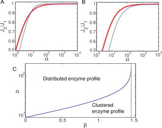
Figure 9: (A,B) Comparison of the reaction efficiency for clustered (thick red line) and distributed (thin blue line) $E_{2}$ enzymes reveals a qualitatively different behavior in different $\beta$ ranges. For $\beta=0.1$ (A) a cross-over is observed at which the profile with the higher efficiency changes. For $\beta=5$ (B) clustering is preferable for all values of $\alpha$. (C) The transition value of $\alpha$ dividing the regimes where the clustered or uniform profiles achieve a higher reaction flux, found by solving $(J_{2}/J_{1})_{\rm u}=(J_{2}/J_{1})_{\rm c}$ numerically. Above the critical $\beta_{c}\approx 1.4$ (dashed line) the transition disappears and the clustering of enzymes is always more efficient.

The reaction fluxes obtained by solving this system for uniform and clustered enzyme configurations are

$$\left(\frac{J_{2}}{J_{1}}\right)_{\rm u} =\frac{\alpha}{\alpha+\beta}\left(1-{\rm sech}\sqrt{\alpha+\beta}\right),$$ (16)

$$\left(\frac{J_{2}}{J_{1}}\right)_{\rm c} =\frac{\alpha}{\alpha+\sqrt{\beta}\ {\rm coth}\sqrt{\beta}}.$$ (17)

Figure 9A and B confirms that there is a difference in whether the clustered or uniform profile is more efficient in different regimes of $\beta$, in keeping with our expectations. Figure 9C plots the critical value of $\alpha$ as a function of $\beta$, and demonstrates that the transition disappears at a finite value of $\beta_{c}\approx 1.4$. When $\beta>\beta_{c}$ the clustered configuration always achieves a higher reaction flux.

SUPPLEMENTARY MATERIAL

S1 Equivalence of expressions for the reaction efficiency

The reaction-diffusion equation leads us to define the reaction efficiency according to the Eq. 3 of the main text,

$$\frac{J_{2}}{J_{1}}=\int\alpha e(\mathbf{r})\frac{\rho(\mathbf{r})}{1+\gamma\rho(\mathbf{r})}{\rm d}\mathbf{r}.$$ (S1)

Here we show that the alternative expression (Eq. 5 of the main text)

$$\frac{J_{2}}{J_{1}}=\int_{0}^{\infty}P(E)p_{\rm r}(E){\rm d}E,$$ (S2)

which arises from the examination of individual intermediate trajectories, can be derived from Eq. S1 in the linear regime where $\gamma\to 0$.

We begin by reformulating the steady-state density $\rho({\mathbf{r}})$ in terms of trajectories of diffusing molecules of intermediate. We denote the diffusive trajectory of a single intermediate molecule, in the absence of any $E_{2}$ enzymes, as $\{\mathbf{r}(t)\}$. Such a trajectory has associated with it a time $t_{\rm escape}$ after which the trajectory is terminated, either by escape across the system boundary or loss to a secondary pathway. The reintroduction of $E_{2}$ enzymes according to the distribution $e({\mathbf{r}})$ leads to an instantaneous propensity for conversion to the correct product at each point along the trajectory of $\alpha e(\mathbf{r}(t))$. Thus the survival probability $S(t|\{\mathbf{r}(t)\})$ that an intermediate molecule on the trajectory $\{\mathbf{r}(t)\}$ has not undergone a reaction with $E_{2}$ before the time $t$ follows $\dot{S}(t|\{\mathbf{r}(t)\})=-\alpha e(\mathbf{r}(t))S(t|\{\mathbf{r}(t)\})$. This equation can be integrated to yield

$$S(t|\{\mathbf{r}(t)\})=\exp\left[-\alpha\int_{0}^{t}{\rm d}t^{\prime}\ e(\mathbf{r}(t^{\prime}))\right],\ \ t\leq t_{\rm escape}.$$ (S3)

At steady state, each trajectory $\{\mathbf{r}(t)\}$ of an intermediate molecule will make a contribution to the total intermediate density at point $\mathbf{r}$ that depends on the total time that the trajectory spends at $\mathbf{r}$, weighted by the probability that the intermediate molecule has not yet undergone a reaction prior to each return to $\mathbf{r}$. This later weighting factor is simply the survival probability $S(t|\{\mathbf{r}(t)\})$. Therefore, the local enzyme density can be rewritten as

$$\rho(\mathbf{r})=\int{\rm d}\{\mathbf{r}(t)\}\ p(\{\mathbf{r}(t)\})\int_{0}^{t_{\rm escape}}{\rm d}t\ S(t|\{\mathbf{r}(t)\})\delta\left[\mathbf{r}-\mathbf{r}(t)\right],$$ (S4)

where the inner integral is the weighted time spent by a single trajectory at $\mathbf{r}$, and the outer integral sums over the contributions of all possible trajectories weighted by the probability $p(\{\mathbf{r}(t)\})$ of a specific trajectory $\{\mathbf{r}(t)\}$ occurring. Substituting Eqs. S4 and S3 into Eq. S1 and changing the order of integration, we find

$$\frac{J_{2}}{J_{1}} =\int{\rm d}\{\mathbf{r}(t)\}\ p(\{\mathbf{r}(t)\})\int_{0}^{t_{\rm escape}}{\rm d}t\int{\rm d}\mathbf{r}\ \alpha e(\mathbf{r})e^{-\alpha\int_{0}^{t}{\rm d}t^{\prime}\ e(\mathbf{r}(t^{\prime}))}\delta\left[\mathbf{r}-\mathbf{r}(t)\right]$$

$$=\int{\rm d}\{\mathbf{r}(t)\}\ p(\{\mathbf{r}(t)\})\int_{0}^{t_{\rm escape}}{\rm d}t\ \alpha e(\mathbf{r}(t))e^{-\alpha\int_{0}^{t}{\rm d}t^{\prime}\ e(\mathbf{r}(t^{\prime}))}$$

$$=\int{\rm d}\{\mathbf{r}(t)\}\ p(\{\mathbf{r}(t)\})\int_{0}^{t_{\rm escape}}{\rm d}t\ \frac{\rm d}{{\rm d}t}\left[-e^{-\alpha\int_{0}^{t}{\rm d}t^{\prime}\ e(\mathbf{r}(t^{\prime}))}\right]$$

$$=\int{\rm d}\{\mathbf{r}(t)\}\ p(\{\mathbf{r}(t)\})\left[1-e^{-\alpha\int_{0}^{t_{\rm escape}}{\rm d}t^{\prime}\ e(\mathbf{r}(t^{\prime}))}\right].$$ (S5)

Finally, defining $E=\int_{0}^{t_{\rm escape}}{\rm d}t\ e(\mathbf{r}(t))$ we can change the variable of integration from $\{\mathbf{r}(t)\}$ to $E$, recovering

$$\frac{J_{2}}{J_{1}}=\int_{0}^{\infty}P(E)(1-e^{-\alpha E}){\rm d}E.$$ (S6)

S2 One dimension including a competing pathway

We consider the rescaled reaction diffusion equation as stated in the main text

$$0=\partial x^{2}\rho(x)-\alpha e(x)\rho(x)-\beta\rho(x),$$ (S7)

with the source boundary conditions $\partial_{x}\rho(x)|_{x=0}=-1$. Below we consider the cases of reflecting ($\partial_{x}\rho(x)|_{x=1}=0$) and absorbing ($\rho(x)|_{x=1}=0$) boundaries at $x=1$.

S2.1 Reflecting boundary, $\partial_{x}\rho(x)|_{x=1}=0$

S2.1.1 Clustered enzyme profile

The enzyme profile is taken to be clustered at some point $x_{0}$, $e_{\rm c}(x)=\delta(x-x_{0})$. In the end we take the limit $x_{0}$ goes to zero, leading to a clustering of $E_{2}$ at the origin. We divide the system into two parts, part $I$ where $x<x_{0}$ and part $II$ where $x>x_{0}$. In each part Eq. S7 reduces to

$$0=\partial x^{2}\rho(x)-\beta\rho(x),$$ (S8)

which has the solution

$$\rho_{i}(x)=A_{i}e^{\sqrt{\beta}x}+B_{i}e^{-\sqrt{\beta}x}$$ (S9)

with $i=\{I,II\}$. Applying the boundary conditions at $x=0$ and $x=1$ yields

$$A_{I}-B_{I}=(\sqrt{\beta})^{-1}\qquad A_{II}e^{\sqrt{\beta}}-B_{II}e^{-\sqrt{\beta}}=0.$$ (S10)

In order to determine all constants we impose two additional conditions, firstly the matching condition of the concentration of intermediates at $x_{0}$, $\rho_{I}(x_{0})=\rho_{II}(x_{0})$ leading to

$$A_{I}e^{\sqrt{\beta}x_{0}}+B_{I}e^{-\sqrt{\beta}x_{0}}=A_{II}e^{\sqrt{\beta}x_{0}}+B_{II}e^{-\sqrt{\beta}x_{0}}$$ (S11)

The second condition, which captures particle conservation in the system, is found by integrating Eq. S7 from $x_{0}-\epsilon$ to $x_{0}+\epsilon$ and taking the limit of small $\epsilon$,

$$\lim_{\epsilon\to 0}\bigg{(}(\partial_{x}\rho_{II}(x))_{x_{0}+\epsilon}-(\partial_{x}\rho_{I}(x))_{x_{0}-\epsilon}-\alpha\rho(x_{0})-\beta\int_{x_{0}-\epsilon}^{x_{0}+\epsilon}\rho(x)dx\bigg{)}=0.$$ (S12)

The last term on the left hand side vanishes in the limit $\epsilon\rightarrow 0$. This leads to the expression

$$\bigg{[}A_{II}e^{\sqrt{\beta}x_{0}}-B_{II}e^{-\sqrt{\beta}x_{0}}-\bigg{(}A_{I}e^{\sqrt{\beta}x_{0}}+B_{I}e^{-\sqrt{\beta}x_{0}}\bigg{)}\bigg{]}-\frac{\alpha}{\sqrt{\beta}}\bigg{(}A_{I}e^{\sqrt{\beta}x_{0}}+B_{I}e^{-\sqrt{\beta}x_{0}}\bigg{)}=0.$$ (S13)

Calculate the reaction current yields

$$\frac{J_{2}}{J_{1}}=\alpha\int_{0}^{1}\delta(x-x_{0})\rho(x)dx=\alpha(A_{II}e^{\sqrt{\beta}x_{0}}+B_{II}e^{-\sqrt{\beta}x_{0}})$$ (S14)

After some straightforward algebra we arrive at expressions for all four constants $\{A_{I},A_{II},B_{I},B_{II}\}$. Last we plug them into the above equation and take the limit $x_{0}\rightarrow 0$,

$$\bigg{(}\frac{J_{2}}{J_{1}}\bigg{)}_{\rm c}=\frac{\alpha}{\alpha+\beta^{\frac{1}{2}}\tanh(\beta^{\frac{1}{2}})}.$$ (S15)

S2.1.2 Uniform enzyme profile

The reaction diffusion equation with a uniform enzyme profile $e_{\rm u}(x)=1$ reads

$$0=\partial x^{2}\rho(x)-(\alpha+\beta)\rho(x).$$ (S16)

The solution is given by

$$\rho(x)=Ae^{\sqrt{\alpha+\beta}x}+Be^{-\sqrt{\alpha+\beta}x}$$ (S17)

Applying the boundary conditions at $x=0$ and $x=L$ leads to the conditions

$$A-B=(\sqrt{\alpha+\beta})^{-1}\qquad Ae^{\sqrt{\alpha+\beta}}-Be^{-\sqrt{\alpha+\beta}}=0.$$ (S18)

Similarly to above, the constants $A$ and $B$ can be obtained straightforwardly, and the efficiency of the pathway is

$$\bigg{(}\frac{J_{2}}{J_{1}}\bigg{)}_{\rm u}=\alpha\int_{0}^{1}\rho(x)dx=\frac{\alpha}{\alpha+\beta}$$ (S19)

S2.2 Absorbing boundary, $\rho(x)|_{x=1}=0$

The approach is very similar to the one the preceding section. The only difference, however, is that the boundary condition $\rho(x)|_{x=1}=0$ leading to a slightly different second condition for the clustered enzymes

$$A_{II}e^{\sqrt{\beta}}+B_{II}e^{-\sqrt{\beta}}=0.$$ (S20)

Likewise, we obtain

$$Ae^{\sqrt{\alpha+\beta}}-Be^{-\sqrt{\alpha+\beta}}=0$$ (S21)

as the second boundary condition for the uniformly distributed enzymes. Similarly, to the approach in section S2.1.1 and S2.1.2, respectively the corresponding efficiency for the clustered case is given by

$$\bigg{(}\frac{J_{2}}{J_{1}}\bigg{)}_{c}=\frac{\alpha}{\alpha+\beta^{\frac{1}{2}}\coth(\beta^{\frac{1}{2}})}$$ (S22)

and for the uniform case

$$\bigg{(}\frac{J_{2}}{J_{1}}\bigg{)}_{u}=\frac{\alpha}{\alpha+\beta}(1-\text{sech}(\sqrt{\alpha+\beta})).$$ (S23)

S3 Enzyme exposure probability distribution in 1D

As shown in the main text, the efficiency of the pathway in terms of the enzyme exposure probability distribution $P(E)$ reads

$$\frac{J_{2}}{J_{1}}=1-\int_{0}^{\infty}P(E)e^{-\alpha E}dE=1-\frac{J_{\rm{loss}}}{J_{1}}.$$ (S24)

To obtain an exact expression of $P(E)$ for the respective case it is convenient to calculate the inverse Laplace transformation of $J_{\rm{loss}}/J_{1}$ with respect to $\alpha$. We have seen above that the expression for the efficiency often has the form $\alpha/(\alpha+f(\beta))$; hence the loss term is $f(\beta)/(\alpha+f(\beta))$. The inverse Laplace transformation is easily obtained and has the form

$$P(E)=f(\beta)e^{-f(\beta)E}.$$ (S25)

For the case of a reflecting outer boundary we therefore have for the uniform enzyme profile, $f(\beta)=\beta$ and thus $P_{\rm u}(E)=\beta e^{-E\beta}$; for the clustered enzyme profile, $f(\beta)=\beta^{\frac{1}{2}}\tanh\beta^{\frac{1}{2}}$ and $P_{\rm c}(E)=\beta^{\frac{1}{2}}\tanh\beta^{\frac{1}{2}}e^{-E\beta^{\frac{1}{2}}\tanh\beta^{\frac{1}{2}}}$.

In the case of an absorbing boundary, the clustered distribution also gives rise to a similar expression for the efficiency, with $f(\beta)=\beta^{\frac{1}{2}}\coth\beta^{\frac{1}{2}}$ and thus $P_{\rm c}(E)=\beta^{\frac{1}{2}}\coth\beta^{\frac{1}{2}}e^{-E\beta^{\frac{1}{2}}\coth\beta^{\frac{1}{2}}}$. However, with a uniform distribution the loss flux does not have the form discussed above, and thus the calculation of the inverse Laplace transformation is more involved. We rewrite Eq. S23 and use Eq. S24 to obtain

$$\bigg{(}1-\frac{J_{2}}{J_{1}}\bigg{)}=\frac{J_{\rm{loss}}}{J_{1}}=\frac{\alpha}{(\alpha+\beta)\cosh(\sqrt{\alpha+\beta})}+\frac{\beta}{\beta+\alpha}.$$ (S26)

Where the second term has the form as we have already discussed above, thus

$$P_{\rm u}(E)={\mathcal{L}}^{-1}\left[\frac{\alpha}{(\alpha+\beta)\cosh(\sqrt{\alpha+\beta})}\right]+\beta e^{-\beta E}.$$ (S27)

The inverse Laplace transformation of the first term is calculated by determining the singularities in terms of $\alpha$ and than calculate their residues by using the Laurent expansion. Finding the poles is here equivalent to determining the roots of the denominator,

$$g(\alpha,\beta)=(\alpha+\beta)\cosh(\sqrt{\alpha+\beta})=0.$$ (S28)

This is satisfied for

$$\alpha=-\beta\qquad\text{and}\qquad\alpha_{n}=-\pi^{2}(n+\frac{1}{2})^{2}-\beta$$ (S29)

for $n\in\mathbb{N}$. And the residues are given by

$$\text{Res}(\alpha g^{-1}(\alpha,\beta)e^{\alpha E},\alpha=-\beta) = -\beta e^{-\beta E}$$

$$\text{Res}(\alpha g^{-1}(\alpha,\beta)e^{\alpha E},\alpha_{0}=-\frac{\pi^{2}}{4}-\beta) = \frac{\pi^{2}+4\beta}{\pi}e^{-(\frac{\pi^{2}}{4}+\beta)E}$$

$$\text{Res}(\alpha g^{-1}(\alpha,\beta)e^{\alpha E},\alpha_{1}=-\frac{-9\pi^{2}}{4}-4\beta) = -\frac{9\pi^{2}+4\beta}{5\pi}e^{-(\frac{9\pi^{2}}{4}+\beta)E}$$

$$\vdots$$

The first term above cancels with the last term in Eq. S27. Combining the remaining terms, we are left with the overall enzyme exposure distribution

$$P_{\rm u}(E)=\sum_{n=0}^{\infty}(-1)^{n}\bigg{(}\frac{(2n+1)^{2}\pi^{2}+4\beta}{(2n+1)\pi}\bigg{)}e^{-(\pi^{2}(n+\frac{1}{2})^{2}+\beta)E}.$$ (S31)

S4 Three dimensions

In three dimensions we impose rotational symmetry and reduce the reaction diffusion equation to depend only on the radial coordinate,

$$r^{-2}\partial_{r}(r^{2}\partial_{r}\rho(r))-\alpha e(r)\rho(r)=0.$$ (S32)

We apply the following boundary conditions, $(4\pi r^{2}\partial_{r}\rho(r))|_{r=0}=-1$ and the outer sphere is absorbing $\rho(r)|_{r=1}=0$.

S4.1 Clustered enzyme profile with absorbing boundary

We again begin by considering a clustered distribution of enzymes, $e_{\rm c}(r)=\frac{\delta(r-r_{0})}{3r_{0}^{2}}$, that has been normalized such that $\int_{0}^{1}4\pi r^{2}e_{\rm c}(r){\rm d}r=4\pi/3$. As in section S2.1.1 we divide the system into two parts, part $I$ for $r<r_{0}$ and part $II$ for $r>r_{0}$. In each part, due to the absence of $E_{2}$ enzymes, the solution of Eq. S32 is

$$\rho_{i}(r)=\frac{A_{i}}{r}+B_{i}$$ (S33)

where $i=\{I,II\}$. Applying the boundary conditions leads to the following two conditions

$$A_{I}=\frac{1}{4\pi}\qquad\text{and}\qquad A_{II}=-B_{II}.$$ (S34)

The remaining two conditions come again from the matching of the concentration at $r=r_{0}$, $\rho_{I}(r_{0})=\rho_{II}(r_{0})$, and the discontinuity of the derivative of the concentration $\rho(r)$ at $r=r_{0}$. Hence we get

$$\frac{1}{4\pi r_{0}}+B_{I}=A_{II}(\frac{1}{r_{0}}-1)$$ (S35)

and

$$-A_{II}+\frac{1}{4\pi}-A_{II}\left[\frac{\alpha}{3}\left(\frac{1}{r_{0}}-1\right)\right]=0.$$ (S36)

With these four conditions Eqs. S34-S36 we obtain after some straightforward algebra the expressions for the four constant $\{A_{I},A_{II},B_{I},B_{II}\}$. Since we do not consider a competing pathway in this model the efficiency of the pathway can also be calculated as

$$\bigg{(}\frac{J_{2}}{J_{1}}\bigg{)}_{\rm c}=1-4\pi(r^{2}\partial_{r}\rho(r))|_{r=1}=4\pi A_{II}=\frac{\frac{\alpha}{3}(1-r_{0})}{r_{0}+\frac{\alpha}{3}(1-r_{0})}.$$ (S37)

S4.2 Uniform enzyme profile with absorbing boundary

For the uniform enzyme profile $e_{\rm u}(r)=1$ the reaction-diffusion equation Eq. S32 reads

$$r^{-2}\partial_{r}(r^{2}\partial_{r}\rho(r))-\alpha\rho(r)=0.$$ (S38)

This is solved by

$$\rho(r)=\frac{1}{r}\bigg{(}Ae^{\sqrt{\alpha}r}+Be^{-\sqrt{\alpha}r}\bigg{)}.$$ (S39)

With the boundary conditions we arrive at the following two conditions: at the origin,

$$A+B=\frac{1}{4\pi},$$ (S40)

and at the absorbing outer boundary,

$$Ae^{\sqrt{\alpha}}+Be^{-\sqrt{\alpha}}=0.$$ (S41)

In the same way as the case of clustered enzymes the efficiency is given by

$$\bigg{(}\frac{J_{2}}{J_{1}}\bigg{)}_{\rm u}=1-4\pi(r^{2}\partial_{r}\rho(r))|_{r=1}=1-\sqrt{\alpha}\rm{csch}(\sqrt{\alpha}).$$ (S42)

S5 Enzyme exposure probability distribution in 3D

Similarly to the one dimensional case the enzyme exposure probability distribution is obtained by the inverse Laplace transformation of the loss current through the boundary. The loss current of the clustered enzyme profile reads

$$\frac{J_{\rm{loss}}}{J_{1}}=\frac{r_{0}}{r_{0}+\frac{\alpha}{3}(1-r_{0})}$$ (S43)

which has the general form discussed in Section S3. Hence the enzyme exposure distribution is

$$P_{\rm c}(E)=\frac{3r_{0}}{1-r_{0}}e^{-\frac{3r_{0}}{1-r_{0}}E}.$$ (S44)

For the uniform enzyme profile, the calculation again proceeds in the same way as described above. We firstly calculate the singularities of the loss current, the roots of $\sinh(\sqrt{\alpha})$, which are given by

$$\alpha_{n}=-(n\pi)^{2}\qquad\text{with}\quad n\in\mathbb{N}.$$ (S45)

This leads then to the following residues

$$\text{Res}(\frac{\sqrt{\alpha}}{\sinh\sqrt{\alpha}}e^{\alpha E},\alpha_{0}=0) = 0$$

$$\text{Res}(\frac{\sqrt{\alpha}}{\sinh\sqrt{\alpha}}e^{\alpha E},\alpha_{1}=-\pi^{2}) = 2\pi^{2}e^{-\pi^{2}E}$$

$$\text{Res}(\frac{\sqrt{\alpha}}{\sinh\sqrt{\alpha}}e^{\alpha E},\alpha_{2}=-4\pi^{2}) = -8\pi^{2}e^{-4\pi^{2}E}$$ (S46)

$$\vdots$$

We assemble all the individual terms and get for the enzyme exposure probability distribution

$$P_{\rm u}(E)=2\sum_{n=1}^{\infty}(-1)^{n+1}(\pi n)^{2}e^{-(n\pi)^{2}E}.$$ (S47)

References

- Srere (1987) P. A. Srere, Annu. Rev. Biochem. 56, 89 (1987).
- Bayer et al. (1998) E. A. Bayer, H. Chanzy, R. Lamad, and Y. Shoham, Curr. Opin. Strut. Biol. 8, 548 (1998).
- de Kok et al. (1998) A. de Kok, A. F. Hengeveld, A. Martin, and A. H. Westphal, Biochim. Biophys. Acta 1385, 353 (1998).
- Campanella et al. (2005) M. E. Campanella, H. Chu, and P. S. Low, Proc. Natl Acad. Sci. USA 102, 2402 (2005).
- Dunn et al. (2008) M. F. Dunn, D. Niks, H. Ngo, T. R. Barends, and I. Schlichting, Trends Biochem. Sci. 33, 254 (2008).
- Gaertner (1978) F. H. Gaertner, Trends Biochem. Sci. 3, 63 (1978).
- Ovádi (1991) J. Ovádi, J. Theor. Biol. 152, 1 (1991).
- Heinrich et al. (1991) R. Heinrich, S. Schuster, and H.-G. Holzütter, Eur. J. Biochem. 201, 1 (1991).
- Cornish-Bowden (1991) A. Cornish-Bowden, Eur. J. Biochem. 195, 103 (1991).
- Mendes et al. (1992) P. Mendes, D. B. Kell, and H. V. Westerhoff, Eur. J. Biochem. 204, 257 (1992).
- Cornish-Bowden and Cárdenas (1993) A. Cornish-Bowden and M. L. Cárdenas, Eur. J. Biochem. 213, 87 (1993).
- Mendes et al. (1996) P. Mendes, D. B. Kell, and H. V. Westerhoff, Biochim. Biophys. Acta 1289, 175 (1996).
- Conrado et al. (2007) R. J. Conrado, T. J. Mansell, J. D. Varner, and M. P. DeLisa, Metab. Eng. 9, 355 (2007).
- van Albada and ten Wolde (2007) S. B. van Albada and P. R. ten Wolde, PLoS Comput. Biol. 3, e195 (2007).
- Mugler et al. (2012) A. Mugler, A. Gotway Bailey, K. Takahashi, and P. R. ten Wolde, Biophys. J. 102, 1069 (2012).
- Conrado et al. (2008) R. J. Conrado, J. D. Varner, and M. P. De Lisa, Curr. Opin. Biotechnol. 19, 492 (2008).
- Dueber et al. (2009) J. E. Dueber, G. C. Wu, G. R. Malmirchegini, T. S. Moon, C. J. Petzold, A. V. Ullal, K. L. J. Prather, and J. D. Keasling, Nat. Biotech. 27, 753 (2009).
- Kufer et al. (2008) S. K. Kufer, E. M. Puchner, H. Gumpp, T. Liedl, and H. E. Gaub, Science 319, 594 (2008).
- Douglas et al. (2009) S. M. Douglas, H. Dietz, T. Liedl, B. Högberg, F. Graf, and W. M. Shih, Nature 459, 414 (2009).
- Niemeyer et al. (2002) C. M. Niemeyer, J. Koehler, and C. Wuerdemann, ChemBioChem 3, 242 (2002).
- Wilner et al. (2009) O. I. Wilner, Y. Weizmann, R. Gill, O. Lioubashevski, R. Freeman, and I. Willner, Nat. Nanotech. 4, 249 (2009).
- Idan and Hess (2013) O. Idan and H. Hess, Curr. Opin. Biotechnol. 24, 606 (2013).
- Delebecque et al. (2011) C. J. Delebecque, A. B. Lindner, P. A. Silver, and F. A. Aldaye, Science 333, 470 (2011).
- Fu et al. (2012) J. Fu, M. Liu, Y. Liu, N. W. Woodbury, and H. Yan, J. Am. Chem. Soc. 134, 5516 (2012).
- Buchner et al. (2013) A. Buchner, F. Tostevin, and U. Gerland, Phys. Rev. Lett. 110, 208104 (2013).
- (26) See Supplementary Material Document for full details of this and following calculations.
- Wilson (1978) J. E. Wilson, Trends Biochem. Sci. 3, 124 (1978).
- John et al. (2011) S. John, J. N. Weiss, and B. Ribalet, PLoS ONE 6, e17674 (2011).
- Sullivan et al. (2003) D. T. Sullivan, R. MacIntyre, N. Fuda, J. Fiori, J. Barrilla, and L. Ramizel, J. Exp. Biol. 206, 2031 (2003).
- Anderson et al. (2005) L. E. Anderson, N. Gatla, and A. A. Carol, Photosynth. Res. 83, 317 (2005).
- Wandersman (1989) C. Wandersman, Mol. Microbiol. 3, 1825 (1989).
- Masters (1984) C. Masters, J. Cell Biol. 99, 222s (1984).
- Simons and Vaz (2004) K. Simons and W. L. C. Vaz, Ann. Rev. Biophys. Biomol. Struct. 33, 269 (2004).
- Rothemund (2006) P. W. K. Rothemund, Nature 440, 297 (2006).