Clustering and optimal arrangement of enzymes in reaction-diffusion systems

Abstract

Enzymes within biochemical pathways are often colocalized, yet the consequences of specific spatial enzyme arrangements remain poorly understood. We study the impact of enzyme arrangement on reaction efficiency within a reaction-diffusion model. The optimal arrangement transitions from a cluster to a distributed profile as a single parameter, which controls the probability of reaction versus diffusive loss of pathway intermediates, is varied. We introduce the concept of enzyme exposure to explain how this transition arises from the stochastic nature of molecular reactions and diffusion.

To efficiently catalyze multi-step biochemical reactions, sets of enzymes have evolved to function synergistically. Cells not only keep concerted control over the concentrations and activities of enzymes in the same pathway, but often also arrange them in self-assembled multi-enzyme complexes Srere1987 . Apart from the large molecular machines (polymerases, ribosomes, spliceosomes), one of the best-studied natural multi-enzyme complexes is the cellulosome, a complex where up to 11 different enzymes are arranged on a non-catalytic scaffolding protein Bayer1998 . This complex is assembled extracellularly by anaerobic bacteria to efficiently break down cellulose, the most abundant organic material on the planet. Similarly, enzyme complexes are used for intracellular metabolism Campanella05 . However, neither the precise consequences of putting enzymes together into complexes are well understood, nor the degree to which complex formation confers a functional advantage in each case Cornish1991 ; Mendes1992 ; Cornish1993 ; Mendes1996 .

It has long been thought that physical association between collaborating enzymes might increase the effective reaction flux, minimize the pool of unwanted intermediate products, allow coordinate regulation by a single effector, and reduce transient timescales Gaertner1978 ; Schuster1991 . However, while enzymatic activity has been studied for over a century, suitable techniques to characterize such effects quantitatively have become available only recently. On the one hand, single-molecule enzymology allows to monitor Xie2001 and manipulate Gumpp09 the activity of individual enzyme molecules. On the other hand, enzyme molecules can be positioned with nanometer precision in artificial systems using “single-molecule cut-and-paste” Kufer08 on 2D surfaces or along 1D channels, and with DNA origami structures even in 3D Niemeyer2008 ; Yan2012 . These experimental developments call for a theoretical analysis of the effects of spatial proximity and arrangement of enzymes, to uncover the principles for the design and optimization of multi-enzyme systems. Such principles could be applied to bio-engineer systems that control biochemical reactions at will, such as for the production of drugs or biofuels Conrado2008 ; Keasling2012 . Related issues also arise in the context of signaling proteins Bray98 , however the functional criteria for the optimization of signaling systems are likely different vanAlbada2007 ; Wolde2012 .

Here, we ask under which conditions it is beneficial to localize enzymes rather than to distribute them. Furthermore, what is the optimal arrangement and how does it depend on the system parameters? We base this study on simple-reaction diffusion models, which permit rigorous quantitative analysis, and assume the steady-state reaction flux is the single critical system property. Interestingly, this already leads to rich physical behavior, with a sharp transition from a regime in which it is optimal to cluster downstream enzymes in the vicinity of upstream enzymes, to a regime in which an extended enzyme profile generates a higher reaction flux. This behavior, which we explain by analyzing the “enzyme exposure” of molecules diffusing in the system, is a result of the stochastic nature of the reactions and diffusion of single molecules.

Clustered enzymes.—

That colocalizing enzymes within the same pathway might indeed improve the efficiency of converting a substrate $S$ into a final product $P$ can be seen by considering a 2-step reaction, $S\xrightarrow{E_{1}}I\xrightarrow{E_{2}}P$, as a minimal model where production of $P$ via an intermediate $I$ is catalyzed by the enzymes $E_{1}$ and $E_{2}$. Let us consider an $E_{1}$ molecule (or a small cluster thereof) as a local source of $I$ molecules and describe the local arrangement of $E_{2}$ enzymes relative to $E_{1}$ by the distribution $e(\mathbf{r})$, normalized such that $E_{T}=\int{\mathrm{d}}^{3}r\,e(\mathbf{r})$ is the total number of $E_{2}$ molecules per $E_{1}$ center. To determine the efficiency of an enzyme arrangement $e(\mathbf{r})$, we need to describe the reaction-diffusion dynamics of the density $\rho(\mathbf{r},t)$ of intermediates. We assume simple diffusion, with coefficient $D$, and standard Michaelis-Menten kinetics Cornish-Bowden2004 for the enzymatic reactions, with catalytic rate $k_{\rm cat}$ and Michaelis constant $K_{M}$ for $E_{2}$. In the low-density regime, where the reaction term becomes linear, we then have

$$\partial_{t}{\rho(\mathbf{r},t)}=D\nabla^{2}\rho(\mathbf{r},t)-\kappa\,e(\mathbf{r})\rho(\mathbf{r},t)$$ (1)

with $\kappa=k_{\rm cat}/K_{M}$ measuring the enzyme efficiency. Intermediates will either react to form product or will be lost, either directly to the extracellular space (for extracellular enzymes) or across the cell membrane. We can implement this possible loss via an absorbing boundary condition, $\rho(r=R,t)=0$, on a sphere with radius $R$ that may be taken to infinity. On the other hand, intermediates are constantly generated by $E_{1}$ at the origin, with an average flux that we denote by $J_{1}$, yielding the source boundary condition $-D(4\pi r^{2}\partial_{r}{\rho})_{r=0}=J_{1}$. In the resulting non-equilibrium steady-state $\rho(\mathbf{r})$, product is generated at the rate

$$J_{2}=\kappa\int_{r<R}\!{\mathrm{d}}^{3}r\,e(\mathbf{r})\rho(\mathbf{r})\;.$$ (2)

Let us assume, for the moment, that enzyme $E_{2}$ is spread over a spherical shell with radius $r_{0}<R$. We then find a total product flux of

$$J_{2}=\frac{J_{1}}{1+\frac{4\pi DR\,r_{0}}{E_{T}\kappa\left(R-r_{0}\right)}}\stackrel{{\scriptstyle R\gg r_{0}}}{{\longrightarrow}}\frac{J_{1}}{1+\frac{4\pi D\,r_{0}}{E_{T}\kappa}}\;.$$ (3)

This result indicates that reducing $r_{0}$—arranging the $E_{2}$ molecules close to the $E_{1}$ center—can dramatically increase the flux if loss of intermediate products is a concern. Whether this effect is biologically relevant crucially depends on the characteristic lengthscale $r_{c}=E_{T}\kappa/4\pi D$ where $J_{2}$ begins to saturate. Enzyme efficiencies can be up to $\kappa\sim 10^{8}\,{\rm M^{-1}s^{-1}}$ (although superefficient enzymes can achieve $\kappa\sim 10^{10}\,{\rm M^{-1}s^{-1}}$Desideri2001 ), while biomolecular diffusion constants are typically larger than $D\sim 10\,{\rm\mu m^{2}s^{-1}}$, such that with $E_{T}\sim 10$ $E_{2}$ molecules per $E_{1}$ center, $r_{c}$ is at most of nanometer scale, comparable to the size of enzymes. Thus even our simplified model, which does not include inter-enzyme interactions such as direct channeling Huang01 , suggests that in realistic biochemical settings, $J_{2}$ will be strongly dependent on the distance between enzymes down to the scale of their own size.

On a microscopic scale, the simple reaction-diffusion description we have used above will break down, since steric effects and the specific enzyme structure become important. Nevertheless, we can exploit the coarse-grained model to address more general questions on a mesoscopic scale. In particular, it is intriguing to ask whether colocalization is in fact the optimal enzyme arrangement, and whether the behavior will change qualitatively when the enzyme kinetics become nonlinear.

Clustered vs. uniform arrangements.—

Let us focus on the one-dimensional version of Eq. 1. This is not only a natural starting point for a theoretical study, but also relevant experimentally, e.g. for “molecular factories” in quasi-1D channels within future “lab-on-a-chip” devices. Specifically, we consider the 1D steady-state $\rho(x)$ of a finite system, $x\in[0,L]$, with source/sink boundaries, $-D(\partial_{x}{\rho})_{x=0}=J_{1}$ and $\rho(L)=0$. We compare different $E_{2}$ enzyme distributions $e(x)$ with the same mean density $\bar{e}=L^{-1}\int_{0}^{L}e(x)dx=E_{T}/L$. The behavior of the system is determined by the dimensionless control parameter $\alpha=\kappa\bar{e}L^{2}/D$, which measures the relative importance of reactions and diffusion in shaping $\rho(x)$. When $\alpha<1$, the system is dominated by diffusion, as the typical reaction timescale $(\kappa\bar{e})^{-1}$ is longer than the typical diffusion time $\sim L^{2}/D$ to the absorbing boundary. Conversely, for large $\alpha$, reactions are fast compared to diffusive escape.

We first compare the reaction flux of clustered enzymes, $e_{\rm c}(x)=\bar{e}\,\delta(x/L)$, and uniform enzymes, $e_{\rm u}(x)=\bar{e}$. As shown in Fig. 1, the clustered configuration achieves a larger flux for $\alpha\lesssim 9$. Surprisingly, for larger $\alpha$, the uniform configuration achieves a higher reaction flux. Thus when reactions are fast compared to diffusion, the intermediates can be consumed more efficiently if $E_{2}$ is uniformly distributed throughout the system.

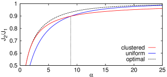
Figure 1: Comparison of the reaction flux achieved by different enzyme profiles. A transition occurs at $\alpha\sim 9$ between regimes in which clustered (red) or uniform (blue) enzyme profiles achieve a higher reaction flux. The optimal mixed enzyme distribution (Eq. 5 with $f=\alpha^{-1/2}$, dashed black line) achieves a still higher $J_{2}$ for intermediate values of $\alpha$.

Enzyme exposure.—

To examine the origin of this transition, we consider the fate of a single $I$ molecule introduced into the system at $t=0$. Whether it will have reacted by time $T$ depends on the concentration of $E_{2}$ enzymes, $e(x(t))$, to which it has been exposed along its trajectory $x(t)$: the probability that it has not reacted is $\exp[-\kappa\int_{0}^{T}\mathrm{d}t\,e(x(t))]$. Therefore, the probability of escaping the system can be decomposed into the likelihood of particular trajectories through the system, and the probability of no reaction occurring along each trajectory. Indeed, the relative likelihoods of escape and reaction can be recaptured if, rather than assuming that $I$ is consumed by the enzyme, we instead propagate a diffusive trajectory until it hits the absorbing boundary at time $\tau$, and subsequently determine whether or not a reaction would have occurred based on the rescaled total enzyme exposure $E=D(L^{2}\bar{e})^{-1}\int_{0}^{\tau}\mathrm{d}t\,e(x(t))$ and reaction probability $p_{\rm r}(E)=1-\exp(-\alpha E)$.

Given the stochasticity of diffusion, a given enzyme arrangement $e(x)$ will lead to a characteristic distribution of enzyme exposure, $P(E)$. For uniformly distributed enzymes, $E$ is simply proportional to the time spent in the system, and $P(E)$ is therefore set by the distribution of escape times at the absorbing boundary $x=1$ for a diffusing particle SI ,

$$P_{\rm u}(E)=\sum_{n=0}^{\infty}\pi(-1)^{n}(2n+1)e^{-\pi^{2}(n+1/2)^{2}E}.$$ (4)

For a clustered configuration the appropriate distribution is found to be $P_{\rm c}(E)=\exp(-E)$ SI . Importantly, these distributions are independent of the reaction rate $\alpha$, which enters into the reaction flux only via the reaction probability $p_{\rm r}(E)$, which is in turn independent of the spatial arrangement of enzymes. Specifically, the reaction flux is given by $J_{2}=J_{1}\int_{0}^{\infty}\!{\mathrm{d}}E\,P(E)\,p_{\rm r}(E)$. Thus it is the interaction of these two distributions which determines which enzyme profile is preferable for a given value of $\alpha$.

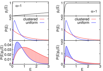
Figure 2: Schematic depiction of the transition from a favorable clustered configuration ($\alpha\ll 1$, left) to the regime in which the uniform profile is preferable ($\alpha\gg 1$, right). (Middle) When enzymes are clustered at $x=0$ $P(E)$ has excess probability, compared to when enzymes are uniformly distributed, at small and large values of $E$. (Bottom) The reaction flux is given by the integral of $P(E)p_{\rm r}(E)$. For $\alpha\ll 1$ the extra probability in the large-$E$ tail of $P(E)$ in the clustered configuration contributes more to $J_{2}$ than probability in the region $E<1$. When $\alpha\gg 1$ only trajectories with $E\ll 1$ are subject to a low reaction probability, leading to a lower $J_{2}$ when enzymes are clustered.

Figure 2 rationalizes the transition observed in Fig. 1. When $\alpha\ll 1$, such that $p_{\rm r}(E\lesssim 1)$ is small, the majority of reaction events correspond to trajectories with large values of $E$. Compared to the uniform configuration, for which $P_{\rm u}(E)\sim\exp(-\pi^{2}E/4)$ for large $E$, the clustered configuration places more probability weight in the large-$E$ tail of $P_{\rm c}(E)$, and thus achieves a higher reaction flux when $\alpha$ is small. In the opposite limit of large $\alpha\gg 10$, only those trajectories with extremely small values of $E\ll 1$ have a significant probability of not reacting. Thus the uniform enzyme profile, for which $P_{\rm u}(E\to 0)\to 0$, becomes preferable. The critical value of the transition, $\alpha\approx 9$, marks the point at which the reaction probability becomes large in the vicinity of the peak of $P_{\rm u}(E)$.

Optimal profiles.—

We have thus far compared only uniformly-distributed and clustered configurations. However, it may be that another enzyme profile is able to achieve a reaction flux which is higher still. We therefore investigated what is the optimal enzyme distribution $e(x)$, for fixed $\bar{e}$, that maximizes the reaction flux $J_{2}$ (or alternatively, minimizes leakage $J_{1}-J_{2}$). A direct analytic optimization of $J_{2}$ over $e(x)$ is not possible because of the non-trivial dependence of $\rho(x)$ on $e(x)$. We therefore studied the optimization of $J_{2}$ numerically on a discretized interval SI .

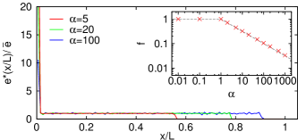
Figure 3: Optimal enzyme density distribution for different values of $\alpha$. Plotted profiles are the result of numerical optimization SI after $4\times 10^{4}$ iterations with a lattice of $100$ sites. Inset: The fraction of enzymes $f$ located at the first lattice site in the numerically-optimized enzyme profile scales as $\alpha^{-1/2}$ for $\alpha>1$.

These data show that for small $\alpha<1$ the clustered configuration, with all enzymes colocalized with the source, is the optimal arrangement. Interestingly, the optimal profile undergoes a transition, distinct from that discussed above, at the critical value $\alpha=1$. For $\alpha>1$, in the optimal profile only a fraction of the available enzymes were clustered; the remaining enzymes were distributed approximately uniformly over an extended region with the enzyme density in this region equal to $\bar{e}$, as shown in Fig. 3.

Motivated by these numerical results we studied enzyme profiles of the form

$$e(x)=\bar{e}\left\{f\delta\left[\frac{x}{L}\right]+1-\Theta\left[\frac{x}{L}-(1-f)\right]\right\},$$ (5)

where $\Theta(x)$ is the Heaviside function, and $f$ is the fraction of enzymes which are clustered. We found that for this restricted class of profiles, the optimal profile indeed undergoes a transition from $f=1$ for $\alpha\leq 1$ to $f=\alpha^{-1/2}$ for $\alpha>1$. Examining the scaling of the fraction of enzymes which are clustered in the numerically-optimized profiles, we find excellent agreement with this $\alpha$-scaling (see Fig. 3 inset). The corresponding reaction flux tracks the envelope of the curves for the clustered and uniform configurations as $\alpha$ is varied (Fig. 1, dashed line).

The two distinct qualitative features of the optimal profile — the peak at $x=0$ and the sharp decrease at $x=L(1-\alpha^{-1/2})$ — can be related to geometry of the system: enzymes cluster in the vicinity of the source, and are excluded from the region nearest to the absorbing boundary. The distance from the end of the uniform enzyme domain to the boundary at $x=L$ scales with the typical diffusion length of substrate molecules in an enzyme density $\bar{e}$, which is $\sim L\alpha^{-1/2}$. If the enzyme concentration were to be uniform, $e(x)=\bar{e}$, substrate molecules that approach within this distance of the absorbing boundary have a high probability of diffusing out of the system rather than reacting. Any enzymes placed in this area contribute little to the reaction flux, and can be used more effectively if relocated closer to the source.

We characterized $P(E)$ for mixed enzyme profiles of the form Eq. 5 by numerically sampling the enzyme exposure of continuous-time random walk trajectories on a lattice until their escape at $x=L$. The resulting distributions for different values of $f$ are shown in Fig. 4. In the extreme cases of $f=1$ and $f=0$ the numerical results reproduce the analytic results of $P_{\rm c}(E)$ and $P_{\rm u}(E)$ above. At intermediate values of $f$, $P(E)$ retains a more pronounced large-$E$ tail than $P_{\rm u}(E)$, while still reducing the probability of extremely small $E$ values relative to $P_{\rm c}(E)$. As $\alpha$ is increased, the relative importance of these two features are reduced and increased, respectively. Thus the optimal $P(E)$ becomes more sharply peaked, corresponding to a smaller $f$.

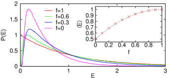
Figure 4: Distributions $P(E)$ estimated from $2\times 10^{6}$ simulated substrate trajectories subjected to an enzyme distribution $e(x_{i})=\bar{e}\left\{fN\delta_{i,1}+1-\Theta\left[\frac{i}{N}-(1-f)\right]\right\}$, with $N=100$.

So far we have considered only the case of linear reaction kinetics. In the nonlinear regime of the Michaelis-Menten kinetics, it is no longer possible to consider individual substrate trajectories independently since the reaction probability of a particular molecule depends on not only the local enzyme concentration but also the substrate density. Nevertheless, a qualitatively similar transition of the optimal enzyme distribution from clustered to distributed will occur provided the enzyme concentration is not so low as to be saturated throughout the entire system, in which case the reaction current becomes independent of enzyme positioning.

Discussion.—

In our model enzymatic pathway, the ultimate fate of each intermediate ($I$) molecule is either to react to product or to escape. For a given enzyme arrangement, the dimensionless parameter $\alpha$ controls the relatively likelihood of these outcomes. Conversely, for each value of $\alpha$ there is an optimal enzyme arrangement that minimizes the loss of intermediates. In the small-$\alpha$ regime, where the reaction is slow and escape is likely, the best enzyme arrangement is a tightly clustered one. As $\alpha$ is increased and the system moves into the reaction-dominated regime, it becomes preferable to relocate some of the available $E_{2}$ enzymes away from the source. The transition of the optimal profile takes place at $\alpha\sim 1$. With a system size of $L\approx 100$ nm, $\alpha$ values in the range of 0.01–100 should be achievable in synthetic systems Kufer08 ; Niemeyer2008 ; Yan2012 . Thus it should be possible to directly test our results experimentally.

Intuitively, these more distant $E_{2}$ molecules may be interpreted as “backup enzymes” intended to catch the fraction of $I$ molecules that were able to diffuse away from the cluster. Indeed, the optimal enzyme arrangement is then akin to a bet-hedging strategy. We have explained this behavior by introducing the integrated “enzyme exposure” along a trajectory. Importantly, the optimal enzyme profile does not necessarily maximize the average enzyme exposure. Rather, it is the matching between the shape of the enzyme exposure distribution and the reaction probability that is key.

Similar effects will also occur in systems with different geometries, including in higher dimensions. Although the magnitude of the changes in reaction flux will vary with the specific system, the underlying physics of the transitions described is extremely generic, determined solely by the statistics of diffusion and reactions. The concept of enzyme exposure provides a general framework for understanding the behavior of many other scenarios.

We have seen that the optimal enzyme distribution is determined by the distributions of timing of reaction and diffusion events. These are intrinsic single-molecule properties. Thus, we expect that the optimal enzyme profile would remain unchanged if we considered instead discrete substrate and enzyme molecules. The only difference is that for finite numbers of enzyme molecules, $e(x)$ cannot be chosen arbitrarily but instead only certain discrete values are permitted. Thus $P(E)$ cannot be varied continuously, but rather one of a specific ensemble of allowed distributions must be chosen. While this will not change the qualitative behavior of the optimal profile as the system parameters are varied, it may quantitatively alter its shape for given parameter values. We leave this as a topic of future studies.

SUPPLEMENTARY MATERIAL

S0.1 Derivation of enzyme exposure distribution $P(E)$

S0.1.1 Uniform configuration

In the case of a uniform enzyme profile, $e_{\rm u}(x)=\bar{e}$, the value of $E$ for an individual substrate trajectory is simply proportional to the time taken to reach the absorbing boundary at $x=L$,

$$E=\frac{D}{L^{2}\bar{e}}\int_{0}^{\tau}{\rm d}t\,e(x(t))=\frac{D}{L^{2}\bar{e}}\int_{0}^{\tau}{\rm d}t\,\bar{e}=\frac{D\tau}{L^{2}}.$$ (S1)

Thus the distribution $P(E)$ is determined by the distribution of escape times at the absorbing boundary, $f(\tau)$. The calculation of the first-passage time distribution for a diffusing particle Redner is included here for completeness. We begin from the renewal equation

$$p(L,t|0,0)=\int_{0}^{t}{\rm d}\tau\,f(\tau)p(L,t|L,\tau).$$ (S2)

Here $p(x,t|x^{\prime},t^{\prime})$ is the probability of a diffusing particle being found at position $x$ at time $t$ given that it was at position $x^{\prime}$ at time $t^{\prime}$, which is given by the solution to the diffusion equation on the semi-infinite domain $x\geq 0$ with a reflecting boundary at $x=0$,

$$p(x,t|x^{\prime},t^{\prime})=\frac{1}{\sqrt{4\pi D(t-t^{\prime})}}\left[e^{-\frac{(x-x^{\prime})^{2}}{4D(t-t^{\prime})}}+e^{-\frac{(x+x^{\prime})^{2}}{4D(t-t^{\prime})}}\right].$$ (S3)

Taking the Laplace transform of Eq. S2 with respect to $t$ we obtain

$$\tilde{f}(z)=\frac{\tilde{p}(L,z|0,0)}{\tilde{p}(L,z|L,0)}.$$ (S4)

Substituting in the Laplace transform of $p(x,t|x,t^{\prime})$ with respect to $t-t^{\prime}$,

$$\tilde{p}(x,z|x^{\prime},0)=\frac{1}{\sqrt{4Dz}}\left[e^{-(x-x^{\prime})\sqrt{\frac{z}{D}}}+e^{-(x+x^{\prime})\sqrt{\frac{z}{D}}}\right],$$ (S5)

we find $\tilde{f}(z)={\rm sech}\sqrt{zL^{2}/D}$. The escape time distribution $f(\tau)$ can be recovered by noting that $\tilde{f}(z)$ has an infinite series of poles at $z=-\frac{\pi^{2}D}{L^{2}}(n+1/2)^{2}$ for $n=0,1,2\dots$, with associated residues $(-1)^{n}(2n+1)\pi D/L^{2}$, yielding

$$f(\tau)=\frac{\pi D}{L^{2}}\sum_{n=0}^{\infty}(-1)^{n}(2n+1)e^{-\pi^{2}(n+1/2)^{2}\tau D/L^{2}}.$$ (S6)

Equation 4 of the main text follows from applying Eq. S1.

S0.1.2 Clustered configuration

To calculate $P(E)$ for the clustered enzyme configuration we consider the enzyme profile

$$e(x)=\begin{cases}\frac{\bar{e}L}{\delta x}&0\leq x<\delta x\\ 0&\delta x\leq x<L\end{cases}.$$ (S7)

Thus for any given trajectory, $E$ is related to the total time $T$ spent in the region $0\leq x<\delta x$ by $E=DT/(L\delta x)$.

Molecules are introduced into the system at $x=0$. The distribution of times at which the intermediate leaves the region $0\leq x<\delta x$ for the first time, $f_{1}(\tau)$, can be calculated as described in the previous section, and is given by Eq. S6 with L replaced by $\delta x$. Once the molecule has left the domain of enzymes, it can either diffuse to $x=L$ and escape from the system, or can diffuse back into the domain $x<\delta x$. The latter will occur with probability $p_{\rm ret}=1-\epsilon/(L-\delta x)$ if the molecule is initially located at a small displacement $+\epsilon$ from the boundary $x=\delta x$ Redner . For a molecule which re-enters the domain $0\leq x<\delta x$, the distribution of times until it subsequently leaves again can be calculated via the procedure described above. Assuming once again a small displacement $-\epsilon$, the escape time distribution $f_{2}(\tau)$ satisfies the corresponding renewal equation

$$p(\delta x,t|\delta x-\epsilon,0)=\int_{0}^{t}{\rm d}\tau\,f_{2}(\tau)p(\delta x,t|\delta x,\tau),$$ (S8)

and has the Laplace transform

$$\tilde{f}_{2}(z)=\frac{\cosh\left[(\delta x-\epsilon)\sqrt{z/D}\right]}{\cosh\left[\delta x\sqrt{z/D}\right]}.$$ (S9)

Since multiple rounds of return are possible, the overall distribution of times spent in the domain $0\leq x<\delta x$ can be expressed in terms of a series of convolutions,

$$f(T)=(1-p_{\rm ret})f_{1}(T)+p_{\rm ret}(1-p_{\rm ret})\int_{0}^{T}{\rm d}\tau^{\prime}\,f_{1}(\tau^{\prime})f_{2}(T-\tau^{\prime})\\ +p_{\rm ret}^{2}(1-p_{\rm ret})\int_{0}^{T}\int_{\tau^{\prime}}^{T}{\rm d}\tau^{\prime\prime}{\rm d}\tau^{\prime}\,f_{1}(\tau^{\prime})f_{2}(\tau^{\prime\prime}-\tau^{\prime})f_{2}(T-\tau^{\prime\prime})+\dots$$ (S10)

In Eq. S10, the first term represents the probability that the molecule spends a time $T$ traversing the domain containing enzymes and then escapes from the system; the second term represents the probability that the molecule returns to the domain $0\leq x<\delta x$ once after it initial leaves, and spends a total time $T$ in the domain; the third term contains the probability that the molecule returns twice, and so on.

Equation S10 can be expressed concisely in the Laplace domain,

$$\tilde{f}(z)=(1-p_{\rm ret})\tilde{f}_{1}(z)\sum_{n=0}^{\infty}\left[p_{\rm ret}\tilde{f}_{2}(z)\right]^{n}=\frac{(1-p_{\rm ret})\tilde{f}_{1}(z)}{1-p_{\rm ret}\tilde{f}_{2}(z)}.$$ (S11)

Substituting in the expressions for $p_{\rm ret}$ and $\tilde{f}_{i}(z)$, taking the limit $\epsilon\to 0$, we ultimately find that for small $\delta x$

$$\tilde{f}(z)\approx\frac{1}{1+zL\delta x/D},$$ (S12)

for which the inverse Laplace transform can be performed straightforwardly to yield

$$f(T)=\frac{D}{L\delta x}e^{-TD/L\delta x}.$$ (S13)

Transforming from $T$ to $E$, we recover $P(E)=\exp(-E)$. Importantly, while $f(T)$ becomes ill-defined in the limit $\delta x\to 0$, $P(E)$ does not suffer this problem.

S0.2 Numerical optimization of enzyme profiles

We studied the optimization of enzyme profiles using a stochastic algorithm consisting of multiple rounds of modification of the enzyme profile and mixing of the best-performing profiles, as described below. This procedure achieved a higher maximal flux, and required less computation time to converge to this optimal profile, than simulated annealing of the enzyme profile using the same mutation procedure at each iteration.

We discretized the domain $0\leq x\leq L$ into $N$ lattice sites with lattice spacing $dx=L/N$. Each optimization run was initialized with a uniform enzyme distribution, $e(x_{i})=1$ for each of the $i=1..N$ lattice sites. At each iteration of the optimization process, a set of 50 new test profiles were generated by selecting one site at random and moving a random fraction of the enzymes present to another randomly-selected site. For each of these modified enzyme configurations, the steady-state $\rho(x)$ was calculated by solving the system of $N$ discrete reaction-diffusion equations,

$$-\frac{J_{1}}{dx} =\frac{D}{dx^{2}}\left[\rho(x_{2})-\rho(x_{1})\right]-\kappa e(x_{1})\rho(x_{1})$$ (S14a)

$$0 =\frac{D}{dx^{2}}\left[\rho(x_{i+1})-2\rho(x_{i})+\rho(x_{i-1})\right]-\kappa e(x_{i})\rho(x_{i})\ \ {\rm for}\ \ {i=2..N-1}$$ (S14b)

$$0 =\frac{D}{dx^{2}}\left[\rho(x_{N-1})-2\rho(x_{N})\right]-\kappa e(x_{N})\rho(x_{N}).$$ (S14c)

Equations S14a and S14c incorporate the source and sink boundary conditions at $x=0$ and $x=L$ respectively. From each solution $\rho(x)$, the reaction flux is calculated as

$$J_{2}=J_{1}-\frac{D}{dx}\rho(x_{N}).$$ (S15)

The initial enzyme distribution for the next round of modifications is constructed by taking the mean of the 10 enzyme profiles with the highest $J_{2}$ values.

The results shown in Fig. 3 of the main text show the individual enzyme profiles which produced the highest $J_{2}$ throughout the entire optimization process. Multiple realizations of this optimization procedure produced the same optimal profile, suggesting that the observed profiles represent the global optimum. The optimal profiles generated were found to be highly robust to changes in the fineness of the discretization $N$, the number of trial profiles and the number of profiles contributing to the average at each iteration, as well as to the initial enzyme configuration at the start of the optimization.