Quantifying the effect of turbulent magnetic diffusion on the growth rate of the magneto-rotational instability

Abstract

Context. In astrophysics, turbulent diffusion is often used in place of microphysical diffusion to avoid resolving the small scales. However, we expect this approach to break down when time and length scales of the turbulence become comparable with other relevant time and length scales in the system. Turbulent diffusion has previously been applied to the magneto-rotational instability (MRI), but no quantitative comparison of growth rates at different turbulent intensities has been performed.

Aims. We investigate to what extent turbulent diffusion can be used to model the effects of small-scale turbulence on the kinematic growth rates of the MRI, and how this depends on angular velocity and magnetic field strength.

Methods. We use direct numerical simulations in three-dimensional shearing boxes with periodic boundary conditions in the spanwise direction and additional random plane-wave volume forcing to drive a turbulent flow at a given length scale. We estimate the turbulent diffusivity using a mixing length formula and compare with results obtained with the test-field method.

Results. It turns out that the concept of turbulent diffusion is remarkably accurate in describing the effect of turbulence on the growth rate of the MRI. No noticeable breakdown of turbulent diffusion has been found, even when time and length scales of the turbulence become comparable with those imposed by the MRI itself. On the other hand, quenching of turbulent magnetic diffusivity by the magnetic field is found to be absent.

Conclusions. Turbulence reduces the growth rate of the MRI in a way that is the same as microphysical magnetic diffusion.

1 Introduction

A cornerstone in the study of astrophysical fluids is linear stability theory (Chandrasekhar, 1961). An important example is the magneto-rotational instability (MRI, see Balbus & Hawley, 1998), which will also be the focus of the present paper. However, the issue is more general, and there are other instabilities that we mention below. When studying linear stability, one typically considers a stationary solution of the full nonlinear equations, linearizes the equations about this solution, and looks for the temporal behavior of small perturbations (wavenumber $k$) proportional to $e^{\lambda t}$, where $t$ is time and $\lambda(k)$ is generally complex. The real part of $\lambda$ is the growth rate, and $\lambda$ as a function of $k$ is the dispersion relation. Linear stability theory is useful to explain why many astrophysical flows are turbulent (e.g., accretion disks through the MRI or the stellar convection zones through the convective instability).

Linear stability theory is also generalized to study the formation of large-scale instabilities in the presence of turbulent flows; e.g., studies of stability of the solar tachocline where convective turbulence is expected to be present (Arlt et al., 2007; Miesch et al., 2007). Let us first revisit this generalization. In the case of a turbulent flow, there is no stationary state in the usual sense; we can at best expect a statistically steady state. In such a situation, the prescription is to average over, or coarse-grain, the fundamental nonlinear equations (e.g., equations of magnetohydrodynamics) to write a set of effective equations valid for large length and time scales. Typical examples of such averaging include Reynolds averaging (Moffatt, 1978; Krause & Rädler, 1980), the multiscale techniques (Zheligovsky, 2012), and application of the dynamical renormalization group, see, e.g., Goldenfeld (1992). The effective equations themselves depend on the averaging process, and also on the length and time scales to which they are applied. The averaging process can give rise to new terms in the effective equations and it introduces new transport coefficients that are often called turbulent transport coefficients to distinguish them from their microphysical counterparts. An example of such an effective equation is the mean-field dynamo equation which, in its simplest form, has two turbulent transport coefficients: the alpha effect, $\alpha$, and turbulent magnetic diffusivity, $\eta_{\rm t}$. Once the effective equations and the turbulent transport coefficients are known, we apply the standard machinery of linear stability theory to the effective equations to obtain the exponential growth or decay rate of large-scale instabilities in or even because of the presence of turbulence.

This prescription, applied to real turbulent flows turns out to be not very straightforward because of several reasons that we list below: (i) Any spatial averaging procedure will retain some level of fluctuations (Hoyng, 1988). This automatically limits the dynamical range over which exponential growth can be obtained. The larger the size of the turbulent eddies compared with the size of the domain, i.e., the smaller the scale separation ratio, the smaller the dynamical range. A well-known example is the $\alpha$ effect in mean-field electrodynamics (Moffatt, 1978; Krause & Rädler, 1980), which gives rise to a linear instability of the mean-field equations. In direct numerical simulations (DNS), however, the expected exponential growth can only be seen over a limited dynamical range. A second, more recent, example is the negative effective magnetic pressure instability (NEMPI) (Brandenburg et al., 2011), where the magnetic pressure develops negative contributions caused by the turbulence itself (Kleeorin et al., 1989; Kleeorin & Rogachevskii, 1994; Rogachevskii & Kleeorin, 2007). NEMPI could be detected in DNS only for a scale separation ratio of ten or more. (ii) The averaged equation, in addition to the usual diffusive terms, can have higher order derivatives in both space and time (Rheinhardt & Brandenburg, 2012). Such terms become important for a small scale separation ratio that generally reduces the efficiency of turbulent transport (Brandenburg et al., 2008a, 2009; Madarassy & Brandenburg, 2010). So, in general, a simple prescription of replacing the microphysical value of diffusivity by its turbulent counterpart may not work. (iii) There are important conceptual differences between microphysical and turbulent transport coefficients. The turbulent ones must reflect the anisotropies and inhomogeneities of real flows, and they are hence, in general, tensors of rank two or higher. Moreover, a major challenge in this formalism is the actual calculation of the turbulent transport coefficients. For turbulent flows, there is at present no known analytical technique that allows us to calculate them from first principles. A recent breakthrough is the use of the test-field method (Schrinner et al., 2005, 2007; Brandenburg et al., 2008b), which allows us to numerically calculate the turbulent transport coefficients for a large class of flows. Armed with the test-field method, we are now in a position to quantify how accurately the linear stability theory applied to the mean-field equations describes the growth of large-scale instabilities in a turbulent flow. This is the principal objective of this paper.

The magneto-rotational instability (MRI) is a relatively simple axisymmetric (two-dimensional) linear instability of a rotating shear flow in the presence of an imposed magnetic field along the rotation axis. The dispersion relation for MRI is well known. Let us now consider the situation in which we have a turbulent flow (which may have been generated due to MRI with microphysical parameters) in a rotating box in the presence of an axial magnetic field and large-scale shear. What is the dispersion relation for large-scale Let us assume that we can use the dispersion relation for MRI and simply replace the microphysical values of magnetic diffusivity ($\eta$) and kinematic viscosity ($\nu$) by turbulent values, $\eta_{\rm t}$ and $\nu_{\rm t}$, respectively. In that case, the growth rate would be given approximately by

$$\lambda\approx V_{\rm A}(k)k-(\eta_{\rm t}+\eta)k^{2},$$ (1)

where $V_{\rm A}(k)k$ is the growth rate in the non-turbulent, ideal case. For the MRI with Keplerian shear, $V_{\rm A}(k)$ is given in terms of $\tilde{V}_{\rm A}=V_{\rm A}k/\Omega$ with (Balbus & Hawley, 1998)

$$V_{\rm A}(k)^{2}=\left(\tilde{v}_{\rm A}^{2}+{\textstyle{1\over 2}}\right)\left\{\left[1+4{(3-\tilde{v}_{\rm A}^{2})\tilde{v}_{\rm A}^{2}\over(2\tilde{v}_{\rm A}^{2}+1)^{2}}\right]^{1/2}\!\!-1\right\},$$ (2)

where $\tilde{v}_{\rm A}=v_{\rm A}k/\Omega$, $v_{\rm A}$ is the Alfvén speed, $k$ is the wavenumber, and $\Omega$ is the angular velocity. The qualitative validity of turbulent diffusion in MRI was previously demonstrated by Korpi et al. (2010), who focussed attention on the Maxwell and Reynolds stresses in the nonlinear regime, following earlier work by Workman & Armitage (2008) on the combined action of MRI in the presence of forced turbulence. The effect of forced turbulence on the MRI has been studied previously in connection with studies of quasi-periodic oscillations driven by the interaction with rotational and epicyclic frequencies (Brandenburg, 2005). Note also that in Eq. (1) we have assumed that $\nu_{\rm t}+\nu=\eta_{\rm t}+\eta$ which is essentially equivalent to assuming that the turbulent magnetic Prandtl number, $\nu_{\rm t}/\eta_{\rm t}$, is unity because in most astrophysical flows $\nu\ll\nu_{\rm t}$ and $\eta\ll\eta_{\rm t}$. This assumption is supported by DNS studies (Yousef et al., 2003).

There is another important difference between microscopic and turbulent magnetic diffusion. For any linear instability the level of the exponentially growing perturbation depends logarithmically on the strength of the initial field. However, turbulent diffusion implies the presence of turbulence, so there is always some non-vanishing projection of the random velocity and magnetic fields, which will act as a seed such that the growth of the magnetic field is independent of the initial conditions and depends just on the value of the forcing wavenumber and the forcing amplitude. This can become particularly important in connection with the large-scale dynamo instability, which is an important example of an instability that operates especially well in a turbulent system. Again, in that case, turbulence can provide a seed magnetic field to the large-scale dynamo through the action of the much faster small-scale dynamo. This idea was first discussed by Beck et al. (1994) in an attempt to explain the rapid saturation of a large-scale magnetic field in the galactic dynamo.

2 Model

Following earlier work of Workman & Armitage (2008) and Korpi et al. (2010), we solve the three-dimensional equations of magnetohydrodynamics (MHD) in a cubic domain of size $L^{3}$ in the presence of rotation with angular velocity $\bm{\Omega}=(0,0,\Omega)$, a shear flow $\overline{U}^{S}=(0,Sx,0)$ with shear $S=-{3\over 2}\Omega$, and an imposed magnetic field $\bm{B}_{0}=(0,0,B_{0})$. We adopt shear-periodic boundary conditions in the $x$ direction (Wisdom & Tremaine, 1988) and periodic boundary conditions in the $y$ and $z$ directions. We generate turbulence by adding a stochastic force with amplitude $f_{0}$ and a wavenumber $k_{\rm f}$. We have varied $f_{0}$ to achieve different root-mean-square (rms) velocities of the turbulence. Different values of the forcing wavenumber $k_{\rm f}$ will also be considered.

We assume an isothermal gas with sound speed $c_{\rm s}$, so the pressure $p=\rho c_{\rm s}^{2}$ is linearly related to the density $\rho$. The hydromagnetic equations are solved in terms of the magnetic vector potential $A$, the velocity $U$, and the density $\ln\rho$ in the form

$${{\cal D}{}\mbox{\boldmath$A$}{}\over{\cal D}{}t}=-SA_{y}\hat{\mbox{\boldmath$x$}}{}+\mbox{\boldmath$U$}{}\times(\bm{B}+\bm{B}_{0})+\eta\nabla^{2}\mbox{\boldmath$A$}{},$$ (3)

$${{\rm D}{}\mbox{\boldmath$U$}{}\over{\rm D}{}t}=-SU_{x}\hat{\mbox{\boldmath$y$}}{}+{\mbox{\boldmath$J$}{}\times\bm{B}\over\rho}-c_{\rm s}^{2}\mbox{\boldmath$\nabla$}{}\ln\rho-2\bm{\Omega}\times\mbox{\boldmath$U$}{}$$

$$+\mbox{\boldmath$f$}{}+\nu\left(\nabla^{2}\mbox{\boldmath$U$}{}+{\textstyle{1\over 3}}\mbox{\boldmath$\nabla$}{}\mbox{\boldmath$\nabla$}{}\!\cdot\!\mbox{\boldmath$U$}{}+2\mbox{\boldmath${\sf S}$}{}\mbox{\boldmath$\nabla$}{}\ln\rho\right)\!,$$ (4)

$${{\rm D}{}\ln\rho\over{\rm D}{}t}=-\mbox{\boldmath$\nabla$}{}\cdot\mbox{\boldmath$U$}{},$$ (5)

where ${\cal D}{}/{\cal D}{}t=\partial/\partial t+\mbox{\boldmath$U$}{}^{S}\cdot\mbox{\boldmath$\nabla$}{}\,$ is the advective derivative based on the shear flow and ${\rm D}{}/{\rm D}{}t={\cal D}{}/{\cal D}{}t+\mbox{\boldmath$U$}{}\cdot\mbox{\boldmath$\nabla$}{}\,$ is the advective derivative based on the full flow field that includes both the shear flow and the deviations from it, $\bm{B}=\mbox{\boldmath$\nabla$}{}\times\mbox{\boldmath$A$}{}$ is the magnetic field expressed in terms of the magnetic vector potential $A$. In our units, the vacuum permeability $\mu_{0}=1$. The current density $\mbox{\boldmath$J$}{}=\mbox{\boldmath$\nabla$}{}\times\bm{B}$, $\eta$ is the magnetic diffusivity, $\nu$ is the kinematic viscosity, and $f$ is the turbulent forcing function given by

$$\mbox{\boldmath$f$}{}=f_{0}\mbox{Re}\,\{N\mbox{\boldmath$f$}{}_{\bm{k}(t)}\exp[i\bm{k}(t)\cdot\bm{x}+i\phi(t)]\},$$ (6)

where $f_{0}$ denotes the non-dimensional forcing amplitude,

$$\mbox{\boldmath$f$}{}_{\bm{k}}={\bm{k}\times(\bm{k}\times\hat{\mbox{\boldmath$e$}}{})-i|\bm{k}|(\bm{k}\times\hat{\mbox{\boldmath$e$}}{})\over 2\bm{k}^{2}\sqrt{1-(\bm{k}\cdot\hat{\mbox{\boldmath$e$}}{})^{2}/\bm{k}^{2}}},$$ (7)

and $\hat{\mbox{\boldmath$e$}}{}$ is an arbitrary unit vector needed to generate a vector $\bm{k}\times\hat{\mbox{\boldmath$e$}}{}$ that is perpendicular to $\bm{k}$, $\phi(t)$ is a random phase, and $N=f_{0}c_{\rm s}(kc_{\rm s}/\delta t)^{1/2}$, where $f_{0}$ is a nondimensional factor, $k=|\bm{k}|$, and $\delta t$ is the length of the time step. We focus on the case where $|\bm{k}|$ is from a narrow band of wavenumbers with forcing wavenumber $k_{\rm f}$.

The smallest wavenumber that fits into the domain is $k_{1}=2\pi/L$, and we shall use $k_{1}$ as our inverse unit length. Our time unit is given by $\Omega^{-1}$. Non-dimensional quantities will be expressed by a tilde. For example the non-dimensional growth rate is $\tilde{\lambda}=\lambda/\Omega$ and the non-dimensional rms velocity is given by $\tilde{u}_{\rm rms}=u_{\rm rms}k_{1}/\Omega$, and the non-dimensional Alfvén speed is given by $\tilde{v}_{\rm A}=v_{\rm A}k_{1}/\Omega$, where $v_{\rm A}=B_{0}/\sqrt{\rho_{0}}$ is the Alfvén speed based on the strength of the imposed magnetic field and $\rho_{0}$ is the volume averaged density. Furthermore, the non-dimensional forcing wavenumber and turbulent diffusion are given by $\tilde{k}_{\rm f}=k_{\rm f}/k_{1}$ and $\tilde{\eta}_{\rm t}=\eta_{\rm t}k_{1}^{2}/\Omega$, respectively.

We quantify our results in terms of fluid and magnetic Reynolds numbers, as well as the Coriolis number, which are respectively defined as

$$\mbox{\rm Re}=u_{\rm rms}/\nu k_{\rm f},\quad\mbox{\rm Re}_{M}=u_{\rm rms}/\eta k_{\rm f},\quad\mbox{\rm Co}=2\Omega/u_{\rm rms}k_{\rm f}.$$ (8)

In this paper, $u_{\rm rms}$ is the rms velocity before the onset of MRI. We characterize our solutions by measuring $u_{\rm rms}$ and a similarly defined $b_{\rm rms}$, which refers to the departure from the imposed field, again before the onset of MRI. We also use the quantity $B_{\rm rms}$ to characterize the growth of the total field, given by $B_{\rm rms}^{2}\equiv b_{\rm rms}^{2}+B_{0}^{2}$, which we use to define the Lundquist number,

$$\mbox{\rm Lu}=B_{\rm rms}/\sqrt{\rho}\eta k_{\rm f},$$ (9)

At small magnetic Reynolds numbers, $\mbox{\rm Re}_{M}\ll 1$, we would expect $b_{\rm rms}/B_{0}\approx\mbox{\rm Re}_{M}^{1/2}$ (Krause & Rädler, 1980), but in most of our runs we have $\mbox{\rm Re}_{M}\gg 1$, in which case $b_{\rm rms}/\sqrt{\rho_{0}}\approx u_{\rm rms}$. Note that the ratio $\mbox{\rm Lu}/\mbox{\rm Re}_{M}$ is then equal to the ratio of magnetic field to the equipartition value. We also consider horizontally averaged magnetic field, $\overline{\mbox{\boldmath$B$}}{}(z,t)$, as well as its rms value, which is then still a function of time.

The DNS are performed with the Pencil Code, which uses sixth-order explicit finite differences in space and a third-order accurate time-stepping method. We use a numerical resolutions of $128^{3}$ and $256^{3}$ mesh points.

In the following, we discuss the dependence of the growth rate on the anticipated magnetic diffusivity

$$\eta_{\rm t0}\equiv u_{\rm rms}/3k_{\rm f}.$$ (10)

This simple formula was previously found to be a good estimate of the actual value of $\eta_{\rm t}$ (Sur et al., 2008), but this ignores complications from a weak dependence on $k_{\rm f}/k_{1}$ (Brandenburg et al., 2008a), as well as the mean magnetic field (Brandenburg et al., 2008c), which would result in magnetic quenching of $\eta_{\rm t}$. To shed more light onto this uncertainty, we also make use of the quasi-kinematic test-field method of Schrinner et al. (2005, 2007) to calculate the actual value of $\eta_{\rm t}$ based on the measured diagonal components of the magnetic diffusion tensor $\eta_{ij}$, i.e., $\eta_{\rm T}\equiv(\eta_{11}+\eta_{22})/2$. We recall that the evolution of the horizontally averaged magnetic field is governed by just four components of $\eta_{ij}$ (Brandenburg et al., 2008b) and another four components of what is called the $\alpha_{ij}$ tensor, whose components turn out to be zero in all cases investigated in this paper.

3 Results

3.1 Turbulence as a seed of MRI

Let us begin by calculating the growth rate of the large-scale instability from our DNS. The DNS is started with an initial condition where the velocity is initially zero. As a result of the action of the external force, small-scale velocity grows fast and then saturates. This small-scale velocity acts as a seed field for the large-scale MRI. Consequently we see a second growth phase at late times. This is due to the growth (via MRI) of large-scale velocity and magnetic field, both of which show exponential growth at this phase. In Fig. 1 we show this growth for different values of the amplitude of the external force. The growth rate of the large-scale instability can be calculated from the exponentially growing part of these plots.

At late times, $\tilde{u}_{\rm rms}$ saturates near unity, while $\tilde{B}_{\rm rms}$ continues to grow; cf. Fig. 1. Eventually, however, our DNS crash, which is a result of insufficient resolution. Increasing the resolution, we have been able to continue the saturated phase for a somewhat longer time. The results of a higher resolution run are shown as a long-dashed line in Fig. 1, where we used $256^{3}$ mesh points. On the other hand, higher resolution is not crucial for determining the turbulence effects on the MRI, which is why in the following we only present results obtained at a resolution of $128^{3}$ mesh points.

Compared to the non-magnetic case, the magnetic field slightly decreases the saturation level of the forced turbulence before the visible growth of MRI. In addition, the presence of a magnetic field causes $\tilde{u}_{\rm rms}$ to have two plateaus: first at the very beginning and second after $\tilde{B}_{\rm rms}$ reaches the level of $\tilde{u}_{\rm rms}$. The difference can also be seen in averages presented in the Fig. 2, where polarity of the $\overline{B}_{x}$ turns to opposite between the first and second plateau.

Once there is exponential growth, the growth rates of $u_{\rm rms}$ and $B_{\rm rms}$ are, as expected, the same, but they are different for different amplitudes $f_{0}$ of the forcing function, see also Table LABEL:TSetAll. Note also that the runs with the weakest forcing have a slightly faster growth, because the resulting turbulent viscosity and diffusivity are smaller, but they also show a later onset of exponential growth. This in turn is related to a weaker residual projection onto the MRI eigenfunction, simply because the amplitude of the turbulence is lower.

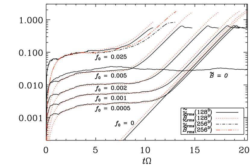
Figure 1: Time dependence of $\tilde{u}_{\rm rms}$ and $\tilde{B}_{\rm rms}$ for runs with $\tilde{k}_{\rm f}=2.2$ (Runs G1-G4 and G7). In addition, sample runs with higher resolution ($256^{3}$), no magnetic fields, and no forcing are included for comparison.

The growth rate $\lambda$ thus calculated is plotted in Fig. 3 as a function of non-dimensionalized $v_{\rm A}$. For comparison, we have also plotted the growth rate calculated from the dispersion relation of MRI, Eq. (1), with a fixed coefficient of magnetic diffusivity $\tilde{\eta}_{\rm fixed}$, where $\tilde{\eta}_{\rm fixed}=\tilde{\eta}+\tilde{\eta}_{\rm t}$. We chose a value for $\eta_{\rm fixed}$ from Run O3 with $\tilde{v}_{\rm A}=0.50$, $\tilde{\eta}_{\rm fixed}=0.01+0.136=0.146$ (see Table LABEL:TSetAll). Both computed runs and the dispersion relation agree reasonably everywhere except with $\tilde{v}_{\rm A}>1.75$, where linear theory predicts no MRI. The positive growth rates in the DNS results in this regime are likely due to another instability such as the incoherent $\alpha$–shear dynamo (Vishniac & Brandenburg, 1997; Mitra & Brandenburg, 2012) and/or the turbulent shear dynamo (Yousef et al., 2008a, b; Heinemann et al., 2011).

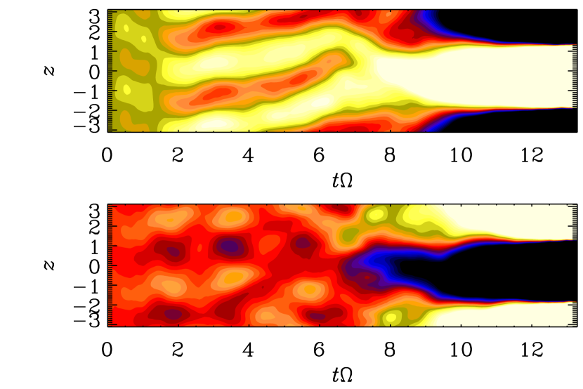
Figure 2: Time dependence of $\ln\overline{B}_{x}$ (top) and $\ln\overline{B}_{y}$ (bottom) for $\tilde{v}_{\rm A}=1.1$ and $\tilde{\eta}=0.01$ (Run O7). Note the different effects of shear on $\overline{B}_{x}$ and $\overline{B}_{y}$.

In the beginning, the components of the horizontally averaged magnetic field $\overline{\mbox{\boldmath$B$}}{}$ are still randomly fluctuating, but at later times, when nonlinear effects begin to play a role, a clear pattern with wavenumber $k=k_{1}$ develops; see Fig. 2. This is expected in this particular run (O7) where the fastest growing mode has a wavenumber close to $k_{1}$. However, we see the same behavior also in other runs in Set O where the theoretically predicted $k_{\rm max}$ varies by more than an order of magnitude, see Table LABEL:TSetAll. By contrast, according to linear theory, the eigenfunction always settles onto the fastest growing one, which would have a wavenumber larger than $k_{1}$.

Figure 3: Dependence of $\tilde{\lambda}$ on $\tilde{v}_{\rm A}$ for the Set O. The dashed line represents the dispersion relation of Eq. (1) with $\tilde{\eta}_{\rm fixed}=\tilde{\eta}+\tilde{\eta}_{t}=0.146$.

3.2 Different ways of varying $\eta_{\rm t}$

To explore the dependence of the solutions on the anticipated turbulent magnetic diffusivity $\eta_{\rm t}$, we consider three sets of runs. In two of them (Sets A and B), we vary $k_{\rm f}$, and in one (Set C) we vary the value of $\Omega$, thus changing Co which was defined in Eq. (8). Given the definition of $\eta_{\rm t0}$ in Eq. (10), we have

$$\tilde{\eta}_{\rm t0}={1\over 3}\tilde{u}_{\rm rms}/\tilde{k}_{\rm f}={2\over 3}\left({k_{\rm f}\over k_{1}}\right)^{-2}\,\mbox{\rm Co}^{-1}.$$ (11)

This shows that increasing either Co or $k_{\rm f}$ or both leads to a decrease of $\tilde{\eta}_{\rm t0}$. We recall that $\tilde{u}_{\rm rms}$ is the value before the onset of MRI and has been estimated by measuring the height of the plateau seen in Fig. 1. We should point out that for small values of $\tilde{k}_{\rm f}$ the length of the plateau becomes rather short, which leads therefore to a significant source of error. The parameters for the three sets of runs are summarized in Table LABEL:TSetAll.

Figure 4: $\tilde{\eta}_{\rm t0}$ versus Coriolis number for $\tilde{v}_{\rm A}=1$, at a resolution of $128^{3}$ mesh points. The solid line is a fit of Eq. (11) into the results of Set C.

In Fig. 4 we plot these three sets of runs in a Co–$\tilde{\eta}_{\rm t0}$ diagram. Looking at Eq. (11), and since $\tilde{k}_{\rm f}=k_{\rm f}/k_{1}=2.3$ is fixed, it is clear that the runs of Set C all fall on a line proportional to $\mbox{\rm Co}^{-1}$. For the other two sets, $\tilde{k}_{\rm f}$ varies. Small values of $\tilde{k}_{\rm f}$ correspond to large values of both Co and $\tilde{\eta}_{\rm t0}$, and vice versa, which is the reason why the other two branches for Sets A and B show an increase of $\tilde{\eta}_{\rm t0}$ for increasing values of Co. Correspondingly, $\tilde{\lambda}$ decreases with increasing Co for Sets A and B, while for Set C, $\tilde{\lambda}$ increases with increasing Co; see Fig. 5.

Figure 5: Growth rate versus Coriolis number for $\tilde{v}_{\rm A}=1$ at a resolution of $128^{3}$ mesh points.

For Sets A and B we show the dependence of the growth rate on $\tilde{k}_{\rm f}$ in Fig. 6. For both sets, $\tilde{\lambda}$ increases with increasing $\tilde{k}_{\rm f}$. This increase is related to the fact for increasing values of $\tilde{k}_{\rm f}$, $\tilde{\eta}_{\rm t0}$ decreases, and thus $\tilde{\lambda}$ shows a mild increase. Indeed, we should expect that $\tilde{\lambda}$ varies with $\tilde{k}_{\rm f}$ like

$$\tilde{\lambda}=\tilde{\lambda}_{0}-\tilde{u}_{\rm rms}/3\tilde{k}_{\rm f},$$ (12)

where in the present case the best agreement with the DNS is obtained when $\tilde{\lambda}_{0}=0.67$ is chosen. This theoretically expected dependency is overplotted in Fig. 6.

Figure 6: Growth rate versus the scale separation $\tilde{k}_{\rm f}$ for $\tilde{v}_{\rm A}=1$, at a resolution of $128^{3}$ mesh points. The solid line shows a fit to the theoretical dependency given by Eq. (12).

Figure 7: Growth rate versus the $\tilde{\eta}_{\rm t0}$ for Sets A–G, at a resolution of $128^{3}$ mesh points.

Let us now turn to relation (1), which predicts a parabolic decline for increasing values of $(\eta_{\rm t}+\eta)k^{2}$. This relation is surprisingly well obeyed; see Fig. 7, where we plot $\tilde{\lambda}$ as a function of $(\eta_{\rm t}+\eta)k^{2}$ for models of all three sets, together with those of Sets D–G listed in Table LABEL:TSetAll.

3.3 Comparison with test-field results

Our results presented so far have demonstrated that in the present problem, the growth of large-scale perturbations is determined by the same equations that describe the growth of MRI but with values of magnetic diffusivity (and viscosity) that are not their microphysical values but turbulent values. Hence, by turning the problem on its head, we have here a new method of calculating the turbulent magnetic diffusivity by measuring the growth rate of the large-scale instability. Such a method would proceed in the following manner. First we would study the growth of the large-scale instability and produce a plot similar to Fig. 1 from which we can calculate the growth rate $\lambda$. Once we know $\lambda$ we can read off $\eta_{\rm t}$ by using Fig. 7. Let us call the turbulent diffusivity, measured in this fashion, $\eta^{\rm MRI}_{\rm t}$. At present, we are already familiar with the well-established test-field method to calculate the turbulent magnetic diffusivity. It then behooves us to compare these two methods, for cases where they both can be applied.

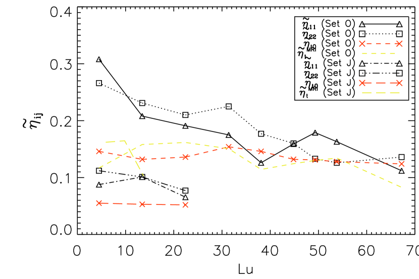
Figure 8: Dependence of $\tilde{\eta}_{11}$ ($\bigtriangleup$) and $\tilde{\eta}_{22}$ ($\square$) as a function of Lu compared to $\tilde{\eta}_{\rm t0}$ and $\eta^{\rm MRI}_{\rm t}$.

Figure 9: Dependence of $\tilde{\eta}_{12}$ ($\square$) and $\tilde{\eta}_{21}$ ($\bigtriangleup$) as a function of Lu.

To apply the test-field method to the present problem, we define averaged quantities by averaging over the horizontal $xy$ plane and choose $z$-dependent test fields which are sines and cosines. In principle the turbulent magnetic diffusivity thus calculated is a second-rank tensor, $\eta_{ij}$. We plot the diagonal and off-diagonal components of this tensor in Figs. 8 and 9, respectively. The off-diagonal elements are close to zero and the diagonal elements are equal to each other and also equal to $\eta_{\rm t0}$. In Table LABEL:TSetAll we list $\tilde{\eta}_{\rm T}=(\tilde{\eta}_{11}+\tilde{\eta}_{22})/2$. Regarding the off-diagonal elements, if any departure from zero is significant, it would be for small values of $\tilde{v}_{\rm A}$, i.e., in the kinematic regime where the effects of magnetic quenching are weak. Earlier DNS of Brandenburg (2005) of MRI in the presence of forcing also showed that $\eta_{12}$ was larger than $\eta_{21}$ by magnitude, but their signs were opposite to those found here. The reason for this difference is however unclear.

3.4 Is there $\eta_{\rm t}$ quenching?

The two methods we have described and compared in the previous subsection now allow us to quantify how turbulent diffusivity is quenched in the presence of the background magnetic field. Quenching of turbulent magnetic diffusivity has been computed analytically (Kitchatinov et al., 1994) and numerically (Yousef et al., 2003), and it has been used in dynamo models (Tobias, 1996; Guerrero et al., 2009). Here, we address this issue by considering the turbulent magnetic diffusivity $\eta^{\rm MRI}_{\rm t}$ and $\eta_{\rm t0}$ as a function of Lu, as done in Fig. 8. In none of the cases do we observe any $\eta_{\rm t}$ quenching.

For Set G we see that $\eta_{\rm t0}$ shows an increase with magnetic field strength (see Table LABEL:TSetAll), which might suggest the possibility of “anti-quenching”. However, in Set G, the value of $\mbox{\rm Re}_{M}$ is also increasing, so the increase in $\eta_{\rm T}$ is really just a consequence of too small values of $\mbox{\rm Re}_{M}$ in the runs with weak magnetic field. This is confirmed by considering the runs in Set O, where $\mbox{\rm Re}_{M}$ is approximately constant and $\eta_{\rm T}$ is then found to be approximately independent of the imposed field strength. It should however be pointed out that the possibility of anti-quenching of $\eta_{\rm t}$ (as well as anti-quenching of the $\alpha$ effect in dynamo theory) has been invoked in the past to explain the observed increase of the ratio of dynamo frequency to rotational frequency for more active stars (Brandenburg et al., 1998). Anti-quenching of $\eta_{\rm t}$ and $\alpha$ was also found for flows driven by the magnetic buoyancy instability (Chatterjee et al., 2011). On the other hand, regular quenching has been found both in the absence of shear (Brandenburg et al., 2008c) as well as in the presence of shear (Käpylä & Brandenburg, 2009). It should therefore be checked whether earlier findings of anti-quenching may also have been affected by too small magnetic Reynolds numbers.

4 Conclusion

Our work has demonstrated several unexpected aspects of turbulent mixing on the operation of the MRI. Firstly, the effect of turbulent magnetic diffusivity seems to be in all aspects equivalent to that of microphysical magnetic diffusivity. This is true even when scale separation is poor, e.g., for $k_{\rm f}/k_{1}=1.5$ or 2.2. This is rather surprising, because in such an extreme case the memory effect was previously found to be important (Brandenburg et al., 2004), which means that higher time derivatives in the mean-field parameterization need to be included (Hubbard & Brandenburg, 2009). Secondly, the simple estimate given by Eq. (10) is remarkably accurate. As a consequence, Eq. (1) provides a quantitatively useful estimate for the effects of turbulence on the growth rate of the MRI. Our simple estimates also agree with results obtained from the test-field method. In principle, there could be other non-diffusive effects resulting from the so-called $\bm{\Omega}\times\mbox{\boldmath$J$}{}$ effect (Rädler, 1969) or the shear–current effect Rogachevskii & Kleeorin (2003, 2004), but our present results show that this does not seem to be the case.

It should also be pointed out that no new terms seem to appear in the momentum equation other than the turbulent viscous force. Of course, this could change if we were to allow for extra effects such as strong density stratification, which could lead to the development of the negative effective magnetic pressure instability (see Brandenburg et al., 2011, and references therein). Furthermore, if there is cross-helicity, there can be new terms in the momentum equation that are linear in the mean magnetic field (Rheinhardt & Brandenburg, 2010). Also kinetic and magnetic helicity could affect our results, although there have not yet been any indications for this from purely hydrodynamic shear flow turbulence (Madarassy & Brandenburg, 2010). Neither the the negative effective magnetic pressure instability nor the $\alpha$ effect dynamo instability are possible in the simple example studied here, because stratification is absent. However, as alluded to in the introduction, they both are examples that have contributed to the motivation of the work presented here.

Appendix A Online material

Table 1: Results for all datasets. Each dataset have been labeled with a specific letter. Some sets share single DNS runs with each other, which have been marked on the table.

Run $\tilde{f}_{0}$ $\tilde{k}_{\rm f}$ $k_{\rm max}$ $\tilde{v}_{\rm A}$ $\mbox{\rm Re}_{M}$ Co Lu $\Omega$ $\tilde{\eta}$ $\tilde{\eta}_{\rm t0}$ $\tilde{\eta}^{\rm MRI}_{\rm t}$ $\tilde{\lambda}$ $\tilde{u}_{\rm rms}$ $\tilde{b}_{\rm rms}$ $\tilde{\eta}_{\rm T}$ N1 0.0000 - 1.0 1.00 - - - 0.10 0.010 - - 0.739 - - - N2 0.0000 - 0.9 1.10 - - - 0.10 0.010 - - 0.729 - - - O1 0.0200 2.2 10.0 0.10 43.79 0.92 4.48 0.10 0.010 0.146 0.117 0.042 0.977 0.843 0.287 O2 0.0200 2.2 3.3 0.30 39.59 1.02 13.45 0.10 0.010 0.132 0.158 0.269 0.883 0.797 0.219 O3 0.0200 2.2 2.0 0.50 40.70 0.99 22.41 0.10 0.010 0.136 0.162 0.435 0.908 0.973 0.200 O4 0.0200 2.2 1.4 0.70 46.35 0.87 31.38 0.10 0.010 0.154 0.150 0.544 1.034 1.161 0.200 O5 0.0200 2.2 1.2 0.85 43.78 0.92 38.10 0.10 0.010 0.146 0.114 0.617 0.977 1.038 0.151 O6 0.0200 2.2 1.0 1.00 39.72 1.01 44.83 0.10 0.010 0.132 0.125 0.615 0.886 0.881 0.160 O7 0.0200 2.2 0.9 1.10 39.33 1.02 49.31 0.10 0.010 0.131 0.129 0.599 0.877 0.850 0.156 O8 0.0200 2.2 0.8 1.20 38.30 1.05 53.79 0.10 0.010 0.128 0.135 0.571 0.854 0.804 0.144 O9 0.0200 2.2 0.7 1.50 37.21 1.08 67.24 0.10 0.010 0.124 0.083 0.447 0.830 0.737 0.124 O10 0.0200 2.2 0.6 1.75 39.55 1.02 78.45 0.10 0.010 0.132 — 0.032 0.882 0.771 0.155 O11 0.0200 2.2 0.5 2.00 40.21 1.00 89.65 0.10 0.010 0.134 — 0.002 0.897 0.759 0.142 O12 0.0200 2.2 0.4 2.50 40.19 1.00 112.07 0.10 0.010 0.134 — 0.001 0.897 0.752 0.168 A1 0.0200 1.5 1.0 1.00 54.45 1.55 64.88 0.10 0.010 0.181 0.107 0.633 0.839 0.785 - A2 0.0200 2.2 1.0 1.00 40.76 0.99 44.83 0.10 0.010 0.136 0.125 0.615 0.909 0.918 - A3 0.0200 3.1 1.0 1.00 29.02 0.70 31.91 0.10 0.010 0.097 0.100 0.639 0.909 0.927 - A4 0.0200 4.1 1.0 1.00 20.24 0.60 24.63 0.10 0.010 0.067 0.098 0.642 0.822 0.767 - A5 0.0200 5.1 1.0 1.00 15.49 0.50 19.62 0.10 0.010 0.052 0.085 0.654 0.789 0.750 - A6 0.0200 10.0 1.0 1.00 6.68 0.30 9.97 0.10 0.010 0.022 0.058 0.681 0.670 0.559 - B1 0.0200 1.5 1.0 1.00 3.52 2.39 6.49 0.10 0.100 0.117 0.069 0.581 0.543 0.453 - B2 0.0200 2.2 1.0 1.00 2.36 1.71 4.48 0.10 0.100 0.079 0.070 0.579 0.525 0.425 - B3 0.0200 3.1 1.0 1.00 1.57 1.30 3.19 0.10 0.100 0.052 0.044 0.605 0.491 0.342 - B4 0.0200 4.1 1.0 1.00 1.12 1.09 2.46 0.10 0.100 0.037 0.034 0.616 0.454 0.284 - B5 0.0200 5.1 1.0 1.00 0.79 0.97 1.96 0.10 0.100 0.026 0.029 0.620 0.403 0.225 - B6 0.0200 10.0 1.0 1.00 0.30 0.66 1.00 0.10 0.100 0.010 0.023 0.626 0.302 0.107 - C1 0.0200 3.1 1.0 1.00 1.40 4.37 9.57 0.30 0.033 0.016 0.066 0.650 0.146 0.122 - C2 0.0200 3.1 1.0 1.00 1.44 2.83 6.38 0.20 0.050 0.024 0.038 0.661 0.226 0.192 - C3 0.0200 3.1 1.0 1.00 1.57 1.30 3.19 0.10 0.100 0.052 0.044 0.605 0.491 0.342 - C4 0.0200 3.1 1.0 1.00 1.57 1.04 2.55 0.08 0.125 0.065 0.038 0.586 0.615 0.392 - C5 0.0200 3.1 1.0 1.00 1.62 0.76 1.91 0.06 0.167 0.090 0.044 0.539 0.845 0.470 - C6 0.0200 3.1 1.0 1.00 1.68 0.48 1.28 0.04 0.250 0.140 0.049 0.451 1.318 0.583 - C7 0.0200 3.1 1.0 1.00 1.78 0.23 0.64 0.02 0.500 0.296 0.087 0.162 2.787 1.131 - D1 0.0200 3.1 1.0 1.00 0.09 9.41 1.37 0.30 0.233 0.007 0.008 0.508 0.068 0.030 - D2 0.0200 3.1 1.0 1.00 0.09 12.71 1.82 0.40 0.175 0.005 0.012 0.562 0.050 0.027 - D3 0.0200 3.1 1.0 1.00 0.09 15.82 2.28 0.50 0.140 0.004 0.013 0.597 0.040 0.023 - E1 0.0010 2.2 1.0 1.00 0.12 33.43 4.48 0.10 0.100 0.004 0.007 0.642 0.027 0.022 - E2 0.0020 2.2 1.0 1.00 0.24 16.69 4.48 0.10 0.100 0.008 0.018 0.632 0.054 0.044 - E3 0.0050 2.2 1.0 1.00 0.59 6.76 4.48 0.10 0.100 0.020 0.018 0.632 0.133 0.109 - E4 0.0200 2.2 1.0 1.00 2.36 1.71 4.48 0.10 0.100 0.079 0.070 0.579 0.525 0.425 - F1 0.0010 3.1 1.0 1.00 0.08 25.70 3.19 0.10 0.100 0.003 0.006 0.643 0.025 0.017 - F2 0.0020 3.1 1.0 1.00 0.16 12.78 3.19 0.10 0.100 0.005 0.017 0.633 0.050 0.033 - F3 0.0050 3.1 1.0 1.00 0.39 5.17 3.19 0.10 0.100 0.013 0.012 0.637 0.124 0.084 - F4 0.0200 3.1 1.0 1.00 1.57 1.30 3.19 0.10 0.100 0.052 0.044 0.605 0.491 0.342 - G1 0.0005 2.2 1.0 1.00 1.16 34.54 44.83 0.10 0.010 0.004 0.008 0.731 0.026 0.025 - G2 0.0010 2.2 1.0 1.00 2.33 17.27 44.83 0.10 0.010 0.008 0.019 0.721 0.052 0.051 - G3 0.0020 2.2 1.0 1.00 4.56 8.82 44.83 0.10 0.010 0.015 0.024 0.716 0.102 0.099 - G4 0.0050 2.2 1.0 1.00 10.88 3.69 44.83 0.10 0.010 0.036 0.036 0.703 0.243 0.235 - G5 0.0080 2.2 1.0 1.00 17.69 2.27 44.83 0.10 0.010 0.059 0.057 0.683 0.395 0.390 - G6 0.0200 2.2 1.0 1.00 40.76 0.99 44.83 0.10 0.010 0.136 0.125 0.615 0.909 0.918 - G7 0.0250 2.2 1.0 1.00 47.92 0.84 44.83 0.10 0.010 0.160 0.120 0.620 1.069 1.086 - J1 0.0200 5.1 3.3 0.30 16.61 0.46 5.89 0.10 0.010 0.055 0.162 0.265 0.847 0.707 0.100 J2 0.0200 5.1 2.0 0.50 15.76 0.49 9.81 0.10 0.010 0.053 0.165 0.432 0.803 0.718 0.101 J3 0.0200 5.1 1.4 0.70 15.53 0.50 13.73 0.10 0.010 0.052 0.102 0.592 0.791 0.743 0.071