A Langevin canonical approach to the dynamics of chiral two level systems. Thermal averages and heat capacity

Abstract

A Langevin canonical framework for a chiral two–level system coupled to a bath of harmonic oscillators is developed within a coupling scheme different to the well known spin-boson model. Thermal equilibrium values are reached at asymptotic times by solving the corresponding set of non–linear coupled equations in a Markovian regime. In particular, phase difference thermal values (or, equivalently, the so–called coherence factor) and heat capacity through energy fluctuations are obtained and discussed in terms of tunneling rates and asymmetries.

I Introduction

Two level systems (TLS) can be considered as a paradigmatic approach found in many different areas of physics and chemistry going, for example, from chiral molecules Harris1978 ; Quack1986 , electron transfer reactions Weiss1999 ; Transferbook ), quantum optics Scullybook to quantum computation Ladd2010 , to name only a few of them. Isolated (two level) systems are very rare in nature and they are very often coupled to a more extended system or thermal bath consisting of many degrees of freedom usually represented by an infinite set of harmonic oscillators. In general, the TLS is linearly coupled to the coordinates of a bath of noninteracting oscillators, whose properties are encoded in their spectral density Leggett1987 . The standard model for such a description is the well–known spin–boson model Weiss1999 . This thermal bath can also be seen as an independent set of identical systems surrounding the tagged one. Within the density matrix formalism, path–integral methods and Bloch–Redfield equations have been proposed and implemented to determine the time evolution of the dissipative TLS Redfield1957 ; Senitzki1963 ; Harris1981 ; Harris1983 ; Hartmann2000 ; Vincenzo2005 ; Isabel2011 . Variational calculations have also been carried out for both the symmetric (or unbiased) Silbey1984 and asymmetric (or biased) cases Harris1985 . Alternatively, according to Feynman in his dynamical theory of the Josephson effect Feynman , it was shown that classical and quantum mechanics may be embedded in the same Hamiltonian formulation by using canonical complex coordinates Strocchi1966 ; Heslot1985 . This procedure was ulteriorly used by Meyer and Miller Meyer1979 starting from an earlier work by McCurdy and Miller McCurdy1978 for electronically non–adiabatic processes. In this work, each electronic state was represented by a pair of classical action-angle variables. In fact, the Meyer–Miller–Stock–Thoss Hamiltonian Meyer1979 ; Stock1997 for a TLS can be rigourously defined after introducing appropriate action angle–coordinates on $S^{2}$ Chruszinskybook , which can be taken to be the true quantum phase space where the dynamics takes place Pedro2013a ; Pedro2013b . Moreover, it can be shown Chruszinskybook that the dynamics derived from this classical formulation is completely equivalent to the quantum one not only for TLS but also for n–level systems.

Very recently, this formalism has also been implemented within the Langevin canonical framework to study the dissipative and stochastic dynamics of chiral molecules and TLSs in general Bargueno2011 ; Penate2012 ; Dorta2012 ; chirality ; Pedro2013a ; Pedro2013b . In this case, the asymmetry of the assumed double well potential model is due to the parity violating energy difference. In particular, the time evolution of the non–isolated chiral TLS has provided thermal average population difference and coherences for incoherent and coherent tunneling. This dynamics is discussed in terms of a critical temperature defined by the maximum of the heat capacity Bargueno2009 ; chirality . It has been proved that this approach is able to reproduce path–integral results beyond the so–called non–interacting blip approximation (NIBA) for a large range of temperatures and by assuming Ohmic friction chirality . Below this critical temperature is where quantum effects are much more important than thermal effects and the coherent regime is well established.

This work can be considered as a next step forward into a more complete dynamical analysis of this open quantum system by focusing on different thermodynamical quantities such as average energies, phase differences and heat capacities issued from a stochastic dynamics. We are not going to consider here a very important topic about anomalies of the heat capacity and refer the reader to some pertinent works Weiss1988 ; Hanggi2008 ; Ingold2009 ; Ingold2012 . Thus, Section II is devoted to briefly introduce the canonical formalism for the isolated and non–isolated TLS. Finite coupling and temperature effects are included by means of noise–induced dynamics via a Caldeira–Leggett–like Hamiltonian. The coupling model is different to the standard spin-boson model since it is the phase difference which is responsible for the coupling with the bath oscillators (in a similar way to the Josephson dynamics). Numerical simulations of this stochastic approach are presented and discussed in Section III, where thermal average energy values as well as phase differences or the so–called coherence factor Stringari2001 are evaluated by assuming an Ohmic regime in a broad range of temperatures. Furthermore, the energy fluctuations expressed in terms of the heat capacity are also showed corroborating the maximum found at the critical temperature. This thermodynamical information is obtained from the stochastic dynamics at asymptotic times where the thermal equilibrium is reached. Derived magnitudes of the energy fluctuations are also the geometric phase and the interference pattern due to the presence of the two enantiomers. In an Appendix, we have also shown that if the coupling with the bath is through the other canonical variable, similar to the spin-boson model, the same asymptotic behavior is clearly obtained but following a different time evolution.

II A Langevin canonical formalism for the stochastic dynamics of chiral two level systems

The isolated TLS is usually modelled by a two-well (asymmetric) potential within the Born-Oppenheimer approximation and described by the phenomenological Hamiltonian

$$\hat{H}=\delta\hat{\sigma}_{x}+\epsilon\hat{\sigma}_{z}$$ (1)

where $\sigma_{x,z}$ stand for the Pauli matrices, $\delta$ accounts for the tunneling rate and $\epsilon$ for the asymmetry of the potential wells due to electroweak parity violation (for a chiral system) or any other biasing term (for example, a polarized electric or magnetic field). In terms of the left and right states (or chiral states), $|L\rangle$ and $|R\rangle$, respectively, these two parameters are given by the matrix elements $\langle L|\hat{H}|R\rangle=-\delta$ (with $\delta>0$) and $2\epsilon=\langle L|\hat{H}|L\rangle-\langle R|\hat{H}|R\rangle$ ($\epsilon$ can be positive or negative).

The time evolution of this system is given by solving the time-dependent Schödinger equation ($\hbar=1$)

$$i\,\partial_{t}|\Psi(t)\rangle=\hat{H}|\Psi(t)\rangle$$ (2)

where the total wave function can be expressed in terms of the chiral states as

$$|\Psi(t)\rangle=a_{L}(t)|L\rangle+a_{R}(t)|R\rangle.$$ (3)

Now, if the complex coefficients are written in polar form as $a_{k}(t)=|a_{k}(t)|e^{i\Phi_{k}(t)}$, where $k$ stands for $R$ or $L$, and the population and phase differences between chiral states are defined as $z(t)\equiv|a_{R}(t)|^{2}-|a_{L}(t)|^{2}$ and $\Phi(t)\equiv\Phi_{R}(t)-\Phi_{L}(t)$, respectively, the average energy in the normalized $|\Psi(t)\rangle$ state is given by

$$H_{0}\equiv\langle\Psi|\hat{H}|\Psi\rangle=-2\delta\sqrt{1-z^{2}}\cos\Phi+2\epsilon z$$ (4)

$H_{0}$ being a Hamiltonian function Quantumbook . Since $z$ and $\Phi$ are a pair of canonically conjugate variables, the Hamilton or Heisenberg equations of motion are derived from $\dot{z}=-\partial H_{0}/\partial\Phi$ and $\dot{\Phi}=\partial H_{0}/\partial z$ to give

$$\dot{z} = -2\delta\sqrt{1-z^{2}}\sin\Phi$$

$$\dot{\Phi} = 2\delta\frac{z}{\sqrt{1-z^{2}}}\cos\Phi+2\epsilon.$$ (5)

Thus, these two non-linear coupled equations are equivalent to Eq. (2). For practical purposes, the adimensional time $t\rightarrow 2\delta\,t$ is frequently used in this context. Thus, the corresponding time scaling implies that the dimensionless Hamiltonian function $H_{0}$ is now expressed as

$$H_{0}=-\sqrt{1-z^{2}}\cos\Phi+\frac{\epsilon}{\delta}z.$$ (6)

Note that the first term of the Hamiltonian function (6) accounts for the tunneling process due to the presence of the oscillatory function and, the second one, for the underlying asymmetry, stressing the fact that two competing processes are present in this simple dynamics. In addition, the ratio between $\epsilon$ and $\delta$ is critical in this dynamics since it provides a way to control the effects of delocalization/localization. In other words, when the tunneling rate is much greater than the bias, the first term of the Hamiltonian (6) predominates and an important delocalization is expected to be present. On the contrary, important asymmetries localize the dynamics in one of the two potential wells.

When dealing with environment interactions consisting of a high number of degrees of freedom, several theoretical treatments are widely used. They are typically classified according to one of the three pictures of quantum mechanics Weiss1999 ; Petruccione2006 : the density matrix formalism and the stochastic Schrödinger equation (interaction and Schrödinger pictures), and the generalized Langevin equation (Heisenberg picture). Within our theoretical scheme, it is clear that the time evolution of the non-isolated, chiral TLS system has to be carried out in the last picture Sanzbook1 ; Sanzbook2 . In this canonical formalism, a Caldeira–Leggett–like Hamiltonian, Leggett1987 where a bilinear coupling between the TLS and the environment is assumed, has been recently developed to study the corresponding dissipative and stochastic dynamics Bargueno2011 ; Penate2012 ; Dorta2012 ; chirality . As stated before, noting that $\Phi$ and $z$ play the role of a generalized coordinate and momentum, respectively, one can straightforwardly derive the following system of coupled Langevin-type dynamical equations Bargueno2011 ; Penate2012 ; Dorta2012 ; chirality

$$\dot{z} = -\sqrt{1-z^{2}}\sin\Phi$$

$$- \int^{t}_{0}\gamma(t-t^{\prime})\dot{\Phi}(t^{\prime})\,dt^{\prime}+\xi(t)$$

$$\dot{\Phi} = \frac{z}{\sqrt{1-z^{2}}}\cos\Phi+\frac{\epsilon}{\delta},$$ (7)

where $\gamma(t)$ is the time-dependent friction (or damping kernel) and $\xi(t)$ the fluctuation force or noise. Note that this approach does not correspond to the standard spin-boson model Weiss1999 . It follows quite closely that employed in the field of condensed matter, in particular, the dynamics of a Josephson junction Weiss1999 . This phase difference is coupled to the degrees of freedom of the degree of the bath which also acts as a source of phase fluctuations. The thermal average of the corresponding cosine function is called the coherence factor Stringari2001 which provides the degree of coherence of the process. In the Appendix, and for completeness, a coupling following the standard spin-boson model is also discussed.

When a Markovian regime is assumed, the usual properties of the fluctuation force (Gaussian white noise) are given by the following canonical thermal averages: $\langle\xi(t)\rangle_{\beta}=0$ (zero average) and $\langle\xi(0)\xi(t)\rangle_{\beta}=mk_{B}T\gamma\delta(t)$ (delta-correlated) where $\beta=(k_{B}T)^{-1}$, $k_{B}$ being Boltzmann’s constant. The friction is then described by $\gamma(t)=2\gamma\delta(t)$, where $\gamma$ is a constant and $\delta(t)$ is Dirac’s $\delta$–function (not to be confused with the $\delta$-parameter describing the tunneling rate). Thus, in this regime, Eqs. (II) read now as follows

$$\dot{z} = -\sqrt{1-z^{2}}\sin\Phi-\gamma\dot{\Phi}(t)+\xi(t)$$

$$\dot{\Phi} = \frac{z}{\sqrt{1-z^{2}}}\cos\Phi+\frac{\epsilon}{\delta}.$$ (8)

The corresponding solutions provide stochastic trajectories for the population and phase differences encoding all the information on the dynamics of the non-isolated, chiral TLS. Interestingly enough it is the fact that from Eqs. (II), an effective Hamiltonian function which explicitly depends on the friction and noise can be extracted from the Hamilton equations given by Eq. (II),

$$H_{\gamma,\xi}(z,\Phi)=-\sqrt{1-z^{2}}\cos\Phi+\frac{\epsilon}{\delta}z+\gamma\Phi\dot{\Phi}-\xi\Phi$$ (9)

which represents the non–conserved energy of the chiral system under the presence of the thermal bath and its mutual coupling as a function of time. This effective energy turns out to be critical for the evaluation of any thermodynamical function such as, for example, the heat capacity. In a certain sense, this information is the alternative way to the more standard one of using the density matrix an/or partition function for the reduced system. It gives us a simple method to evaluate time dependent energy fluctuations.

On the other hand, the connection to the density matrix formalism is readily obtained from the corresponding matrix elements expressed as $\rho_{R,R}=|a_{R}|^{2}$, $\rho_{L,L}=|a_{L}|^{2}$, $\rho_{L,R}=a_{L}a_{R}^{*}$ and $\rho_{R,L}=a_{R}a_{L}^{*}$. Thus, the time average values of the Pauli operators are given by

$$\langle\hat{\sigma}_{z}\rangle_{t} = \rho_{R,R}-\rho_{L,L}=z$$

$$\langle\hat{\sigma}_{x}\rangle_{t} = \rho_{R,L}+\rho_{L,R}=-\sqrt{1-z^{2}}\cos\Phi$$

$$\langle\hat{\sigma}_{y}\rangle_{t} = i\rho_{R,L}-i\rho_{L,R}=\sqrt{1-z^{2}}\sin\Phi,$$ (10)

which is consistent with $\langle\hat{H}\rangle=\delta\langle\hat{\sigma}_{x}\rangle+\epsilon\langle\hat{\sigma}_{z}\rangle$ and

$$\langle\hat{\sigma}_{x}\rangle_{t}^{2}+\langle\hat{\sigma}_{y}\rangle_{t}^{2}+\langle\hat{\sigma}_{z}\rangle_{t}^{2}\leq 1.$$ (11)

where the equal sign holds for the isolated system dynamics.

Several comments are in order when solving numerically Eqs. (II). First, units along this work are dimensionless. By doing this, we are considering a general dynamics where any chiral molecule can be represented. For example, if for a given chiral molecule $\delta=10^{-4}$ meV, we set this value to be $1$ after passing the tunneling rate to inverse of atomic units of time, $3.675\,10^{-5}$. In all the calculation, we have further assumed that $\delta\sim\epsilon$ in order to properly analyze the competition between tunneling and asymmetry or between delocalization and localization, as stated before. With the time step used, $\gamma=0.1$ or $0.01$ (dimensionless rate) is a good parameter for the Ohmic friction. When working on thermodynamic functions, reduced units have been employed, that is, energies and temperatures are divided by $\Delta$ (where $\Delta=\sqrt{\delta^{2}+\epsilon^{2}}$). Second, at high temperatures, $\beta^{-1}\gg\gamma$, thermal effects are going to be predominant over quantum effects which become relevant, in general, at times of the order of or less than the so-called thermal time, $\beta$ (in atomic units). However, at very low temperatures, $\beta^{-1}\ll\gamma$, the noise is usually colored and its auto-correlation function is complex, our approach being no longer valid. In fact, at cold or ultracold regimes, a chiral two level bosonic system could display condensation as well as a discontinuity in the heat capacity (reduced temperatures $k_{B}T/\Delta\leq 1$) Bargueno-pccp . Here, a canonical (Maxwell–Boltzman) distribution is assumed and only classical noise is considered since the ultracold regime is not going to be analyzed. Third, the role of initial conditions has been extensively discussed in the literature (see, for example, Weiss1999 ; Petruccione2006 ); for practical purposes, the chiral system will be prepared in one of its two states, left or right ($z(0)=0.999$ or $-0.999$ in order to avoid initial singularities, and very far from the equilibrium condition), and the initial phase difference $\Phi(0)$ will be uniformly distributed around the interval $[-\pi,\pi]$. Fourth, the stochastic trajectories issued from solving Eq. (II) are dependent on the four dimensional parameter space $(\epsilon,\delta,\gamma,T)$. And fifth, when running trajectories there are some of them visiting ”un-physical” regions, that is, $|z|>1$. This drawback is mainly associated with the intensity of the noise since, for large values of it (which depends on both the temperature and the friction coefficient), the stochastic $z$–trajectories can become unbounded. To overcome this problem, we have implemented a reflecting condition such that when the trajectory reaches $|z|>1$, we change its value to $2-|z|$.

The general strategy consist of solving the pair of non-linear coupled equations (II) for the canonical variables under the action of a Gaussian white noise, which is implemented by using an Ermak–like approach Ermak1980 ; Allenbook . Note that in the Langevin–like coupled equations to be solved, the noise term only appears in the equation of motion of the $z$–variable. The time step used is $10^{-2}$ (dimensionless units) for all the cases analyzed. As noted in Bargueno2011 , unstable trajectories can also be found for certain values of $\epsilon$, $\delta$ and $\gamma$ in the simple case of dissipative but non–noisy dynamics. As this problem persists in case of dealing with stochastic trajectories, not every triplet $(\epsilon,\delta,\gamma)$ gives place to a stable trajectory. In these cases, the time evolution of each individual trajectory is not possible and a previous stability analysis is mandatory. However, in the stable case, a satisfactory description of population differences and coherences have been achieved by running up to $10^{4}$ trajectories as already reported elsewhere chirality .

III Thermodynamics from stochastic dynamics

In general, there are several routes to reach thermodynamical properties such as partition functions, thermal averages, heat capacity, entropy, etc. Very likely, the most popular one is that based on the thermodynamic method coming from the path–integral formalism. An extensive account of this formalism can be found in Weiss’s book Weiss1999 . However, numerical instability problems from the analytic continuation of certain functions lead to some drawbacks. As an alternative way to avoid such problems, it can also be proposed the opposite procedure, that is, the computation of thermodynamics from dynamics which may have some advantages. Thus, partition functions and canonical thermal averages are then calculated when carrying out dynamical calculations for different bias or asymmetry. Analogously, one can also obtain the main equilibrium thermodynamics properties of the non-isolated TLS from the stochastic dynamics at asymptotic times (if the dynamics is ergodic) for a given bias and different temperatures. Furthermore, it is worth stressing that the thermodynamic functions are independent on the friction coefficient in the weak coupling limit. Therefore, our thermodynamical average values coming of solving the corresponding stochastic dynamics are independent on the friction coefficient as time goes to infinity, that is, when the thermal equilibrium with the bath is reached. In the strong coupling limit, this fact no longer holds Ingold2009 .

A previous analysis of the thermodynamics of non-interacting chiral molecules assuming a canonical distribution has been carried out elsewhere Bargueno2009 . In particular, thermal averages of pseudoscalar operators were extensively analyzed. The canonical thermal average of an observable $X$ is defined as $\langle X\rangle_{\beta}=\mathrm{Tr}(\rho_{\beta}X)$ where $\rho_{\beta}=Z^{-1}e^{-\beta H}$, $H$ being given by (1). The quantum partition function $Z$ is given by $Z=2\cosh(\beta\Delta)$ from the eigenvalues of $H$. Moreover, the corresponding averages for the population difference and coherences are then calculated to give

$$\langle z\rangle_{\beta}\equiv\langle\hat{\sigma}_{z}\rangle_{\beta} = \frac{\epsilon}{\Delta}\tanh(\beta\Delta)$$

$$\langle\hat{\sigma}_{x}\rangle_{\beta} = \frac{\delta}{\Delta}\tanh(\beta\Delta).$$ (12)

These populations and coherences have also been evaluated from the stochastic dynamics leading to numerical values in agreement with Eqs. (III) chirality . Furthermore, depending on the temperature, the incoherent and coherent tunneling regimes were fitted to path–integral analytical expressions beyond the NIBA in order to extract information of the frequencies and damping factors of the non–isolated system in its time evolution to thermodynamic equilibrium. The critical temperature issued from the maximum of the heat capacity Bargueno2009 can be considered the threshold temperature where quantum effects become dominant; or in other words, where the coherent regime is well established.

Figure 1: Thermal average of the energy of the chiral TLS as a function of the temperature (dimensionless units). Black points are issued from solving the corresponding non–linear equations of motion, Eqs. (II), and solid line from the thermodynamics function given by Eq. (13). Here, $\delta=\epsilon=1$ and $\gamma$ is 0.1 for $T>1$ and 0.01 for $T<1$.

On the other hand, the thermal average of the energy has been showed to be Bargueno2009

$$\langle E\rangle_{\beta}=E_{0}-\Delta\tanh(\beta\Delta).$$ (13)

Usually, the origin of the energy is taken to be $E_{0}=(\langle L|\hat{H}|L\rangle+\langle R|\hat{H}|R\rangle)/2$. Note that the signature of the thermal average is the global factor $\tanh(\beta\Delta)$, reminiscence of the eigenvalues of the $H$ Hamiltonian (1). This thermodynamical quantity can also be easily extracted from the time evolution of the chiral system from the effective Hamiltonian function defined by Eq. (9) at asymptotic times, that is,

$$\langle E\rangle_{\beta}=\langle H_{\gamma,\xi}(z,\Phi)\rangle_{\beta}$$ (14)

In Fig. 1, the thermal average of the energy (solid line) given by Eq. (13) is plotted versus a wide interval of temperatures going from 0.1 to 200 in units of $\Delta$ (reduced temperatures); black points are the asymptotic values of the non-conserved energy of the chiral system when solving the equations of motion, Eqs. (II), for values of $\delta=\epsilon=1$. The $\gamma$ parameter is fixed at 0.1 for temperatures $T>1$ and 0.01 for $T<1$ in order to facilitate the calculations. Remember that the equilibrium state is independent on $\gamma$ for weak coupling with the bath.

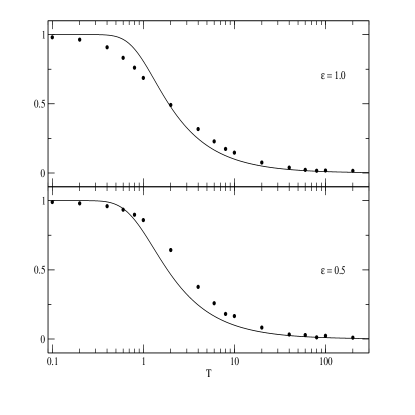
Figure 2: Canonical thermal average of the so–called coherence factor $\langle cos\Phi\rangle_{\beta}$ as a function of the temperature. Here, $\delta=1$, $\epsilon=0.5,1$ and $\gamma$ is 0.1 for $T>1$ and 0.01 for $T<1$.

At this point, one could argue that thermal averages could also be extracted analytically from its definition in standard statistical mechanics, that is,

$$\langle F(z,\Phi)\rangle_{\beta}=\frac{1}{Z_{c}}\int_{-1}^{1}dz\int_{0}^{2\pi}d\Phi F(z,\Phi)e^{-\beta H_{0}(z,\Phi)}$$ (15)

where $F(z,\Phi)$ is a general function of the canonical variables $z$ and $\Phi$ and $H_{0}$ is the Hamiltonian given by Eq. (6). A straightforward analytical integration of the corresponding partition function $Z_{c}$ gives

$$Z_{c}=\frac{4\pi}{\beta\Delta}\,\mathrm{sinh}\beta\Delta$$ (16)

which is quite different from the quantum partition function mentioned above. The corresponding thermal averages of $z$, $E$, $\sigma_{x}$, etc. can also be easily evaluated analytically. The corresponding results are clearly different from the ones previously discussed. In principle, one should expect agreement when the dynamical conditions are approaching those of a classical system (for example, by increasing the temperature).

Special attention deserves the thermal average of $\Phi$ and $\cos\Phi$ Sringari2001, the last average being also called coherence factor, $\langle\cos\Phi\rangle_{\beta}$ (which provides the degree of coherence of the chiral system). In particular, the quantum thermal average of the coherence factor is given by

$$\langle\cos\Phi\rangle_{\beta}=\frac{\sum_{n}\langle n|\cos\Phi|n\rangle e^{-\beta E_{n}}}{\sum_{n}e^{-\beta E_{n}}}$$ (17)

where the sum over $n$ runs only two values, the two eigenstates. The quantum averages of $\cos\Phi$ over these two eigenstates could be carried out following Ref. Carruthers1968 . Here, however, we are going to follow a simpler procedure. Due to the fact the equilibrium values of $\langle z\rangle_{\beta}$ and $\langle\sigma_{x}\rangle_{\beta}$, Eq. (III), are well reproduced from our stochastic calculations, the values of $\langle\cos\Phi\rangle_{\beta}$ could be extracted from those thermal averages. Thus, we have that

$$\langle\cos\Phi\rangle_{\beta}=\frac{(\delta/\Delta)\mathrm{tanh}(\beta\Delta)}{\sqrt{1-(\epsilon/\Delta)^{2}\mathrm{tanh}^{2}(\beta\Delta)}}.$$ (18)

In Fig. 2 we plot both behaviors as a function of the temperature for $\delta=1$ and two values of $\epsilon=0.5,1$. As can be seen, the agreement is fairly good. At very high temperatures, where the classical limit is reached, the tail of the coherence factor is given by

$$\langle\cos\Phi\rangle_{\beta}\simeq\pi^{2}\frac{\delta}{\epsilon}I_{1}(\beta\epsilon)\rightarrow\frac{1}{T}.$$ (19)

if the linear term is retained for the modified Bessel function of first order. This expression is obtained approximately from Eq. (15) when $F(z,\Phi)=cos\Phi$.

Once the stochastic dynamics is well characterized, the next step is to calculate the heat capacity. In thermodynamics, from the knowledge of the partition function, the equilibrium thermodynamical functions are also easily deduced such as the free energy, the entropy, the heat capacity, etc. In particular, the heat capacity at constant volume is expressed for a chiral system as Bargueno2009

$$C_{v}=k_{B}\beta^{2}\Delta^{2}\mathrm{sech}^{2}\beta\Delta$$ (20)

displaying the so-called Schottky anomaly occurring in systems with a limited number of energy levels. This thermodynamic expression for the heat capacity is usually derived from one of the two following expressions

$$C_{v} = \frac{\partial U}{\partial T}$$ (21)

$$= k_{B}\beta^{2}\frac{\partial^{2}Z}{\partial\beta^{2}}$$

where $U$ is the internal energy. For open systems, the coupling to the heat bath defining the temperature is in general finite and weak. The definition of the internal energy is not obvious. Usually, one is inclined to assume that

$$U=\frac{\partial\langle E\rangle_{\beta}}{\partial T}$$ (22)

where this energy is seen as the average energy of the chiral system in the presence of the thermal bath and its mutual interaction. In our context, it is the non–conserved energy given by Eqs. (9) and (14). If we want to follow the second expression, the partition function of the reduced system has to be used. As pointed out previously Hanggi2008 ; Ingold2009 ; Ingold2012 , these two routes may differ yielding different results. In particular, the second route leads to negative values at very low temperatures when dealing with free damped particles. Specific heat anomalies in open quantum systems are nowadays an important topic.

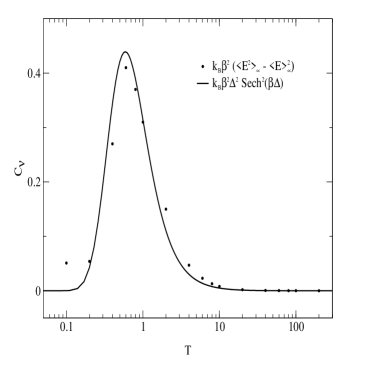
Figure 3: Heat capacity of the chiral TLS issued from the stochastic dynamics (solid points) and from the thermodynamical equilibrium (solid line). Here the choice of parameters are: $\delta=1$, $\epsilon=0.5$ and $\gamma=0.1$ for $T>1$ and 0.01 for $T<1$

In this work, we are going to use a different strategy. The heat capacity is evaluated from the energy fluctuations of the chiral system as

$$C_{v}=\frac{1}{k_{B}T^{2}}\langle(E-\langle E\rangle_{\beta})^{2}\rangle_{\beta}$$ (23)

Following this procedure, the heat capacity is time–dependent till it reaches a constant value at asymptotic times. In Fig. 3, it is shown the heat capacity from Eq. (20) (thermodynamical value, solid line) and from the energy fluctuations through Eq. (23) after propagating the equations of motion at asymptotic times (solid points). In Fig. 4, the time evolution of the corresponding energy fluctuations are also plotted for some different temperatures displaying quite regular oscillations due to the interaction with the bath and the tunneling process. As can be seen, the agreement is fairly good taking into account the semi–log plot of the horizontal axes.

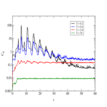
Figure 4: Time dependent energy fluctuations expressed in terms of the heat capacity at four different temperatures, covering a range around the critical value which is $T_{c}=1$ for $\delta=1$ and $\epsilon=0.5$ $\gamma=0.1$ for $T>1$ and 0.01 for $T<1$.

The temperature behavior exhibited by the heat capacity displaying the Schottky anomaly in Fig. 3 leads to the definition of a critical temperature defined by its maximum to be Bargueno2009

$$T_{c}\sim\frac{\Delta}{k_{B}1.2}.$$ (24)

When $T>T_{c}$, the effect of $\epsilon$ is masked by thermal effects which tend to wash out the population difference $z$ (racemization). On the contrary, for $T<T_{c}$, the value of the ratio $\epsilon/\delta$ is critical. If this ratio is close to unity, the whole dynamics is determined by the competition between tunneling and asymmetry or bias. When it is much greater than one, the tunneling process plays a minor role and the dynamics gives place to localization. However, the racemization is always present for ratios much less than one. Given the values of these parameters in our calculation, the critical temperature is $T_{c}\sim 1$ in units of $\Delta$. Thus, the range of temperatures covered in all the calculations takes into account the coherent and incoherent tunneling regimes.

Finally, several magnitudes can also be straightforward derived from the energy fluctuations such as the geometric phase and the diffraction pattern. In Ref. Dorta2012 , it was reported a natural extension of the geometric phase to dissipative two level systems. A further extension it is also possible for these systems but the dynamics is stochastic. Thus, we have that

$$\phi_{g}\equiv\pi+\int_{0}^{\tau}H_{\gamma,\xi}(z,\Phi)dt$$ (25)

where $\tau$ accounts for the period of a complete cycle. Due to the fact that the quantity $H_{\gamma,\xi}(z,\Phi)$ is to be erratic along time, it is better to average over the number of total trajectories in order to have a smooth function with time, the corresponding time integration being easily carried out

$$\langle\phi_{g}\rangle\equiv\pi+\int_{0}^{\tau}\langle H_{\gamma,\xi}(z,\Phi)\rangle dt$$ (26)

In a similar vein, information on interference experiments can be straightforwardly extracted from the probability density of the non-isolated TLS, that is,

$$I\propto|\Phi(t)|1+2|a_{L}(t)||a_{R}(t)|cos\Phi(t)$$ (27)

Now by using the effective Hamiltonian approach here developed, the total intensity of the interference pattern for the Ohmic case is given by

$$I\propto 1+\frac{\epsilon}{z}-H_{\gamma,\xi}(z,\Phi)$$ (28)

IV Final discussion

In this work, we have put on evidence that the stochastic dynamics of a non-isolated chiral TLS, and issued from a classical formalism, is able to reproduce the quantum termodynamical functions such as partition function and heat capacity as well as the so-called coherence factor. The corresponding classical thermodynamical magnitudes calculated from the classical Hamiltonian function are only valid at high temperatures. In other words, we have here a case where a classical stochastic dynamics is able to reproduce the coherent and incoherent regimes taken place in a chiral TLS in presence of a thermal bath. After our analysis, we are describing the coherence regime by means of a classical dynamics. We think this is also a good example where the origin of coherence effects (quantum or classical) here is not so obvious, if not ambiguous Miller2012 . Finally, we have also discussed the difference between the $\Phi$- and $z$-coupling in this dynamics. As should be expected, the asymptotic behavior has to be the same but the time evolution follows different paths.

V Appendix

In this Appendix we derive the stochastic Langevin equations for a two–level system when the system–bath coupling depends of the system population difference instead of the system relative phase. We will explicitly show that, for the dissipative case (that is, for zero temperature), the magnitudes at the equilibrium are independent of the type of coupling considered.

We start with the total Hamiltonian $H=H_{0}+H_{b}+H_{sb}$, where $H_{0}$, given by Eq. (6), is the canonical Hamiltonian for the isolated two–level system,

$$H_{b}=\nobreak\frac{1}{2}\sum_{i}\left(\frac{p_{i}^{2}}{m_{i}}+m_{i}\omega_{i}^{2}x_{i}^{2}\right)$$ (29)

is the Hamiltonian for the bath, which acts as a reservoir, and can be represented as a set of harmonic oscillators, and

$$H_{sb}=\nobreak\sum_{i}\left[\frac{z^{2}d_{i}^{2}}{m_{i}\omega_{i}^{2}}-2d_{i}zx_{i}\right]$$ (30)

expresses an interaction term between the isolated system and the bath, where $d_{i}$ are appropriate coupling constants. We note that when the system–bath coupling is linear in $\Phi$, that is, when the coupling is of the form $\Phi x_{i}$, the dynamics corresponds to that employed in this article and in previous works Bargueno2011 ; Dorta2012 ; chirality . However, in this appendix we investigate the effects of a $zx_{i}$ coupling, as shown in Eq. (30).

After the elimination of the bath degrees of freedom we arrive at the following equations:

$$\dot{z} = -\sqrt{1-z^{2}}\sin\Phi$$

$$\dot{\Phi} = \frac{z}{\sqrt{1-z^{2}}}\cos\Phi+\frac{\epsilon}{\delta}-\int_{0}^{t}\gamma(t-s)\dot{z}ds+\xi(t),$$ (31)

where both the friction kernel and the noise function have the usual definition chirality . Therefore, the only difference with the $\Phi x_{i}$ coupling lies at the dissipative $\gamma\dot{z}$ term.

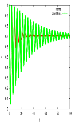
Figure 5: Comparison between $\Phi$-coupling (red line) and $z$-coupling (green line) for the population differences when $\epsilon=\delta=1$ and $\gamma=10^{-1}$. See text for details.

To compare Eqs. (V) with their counterparts given by Eq. (II), we consider pure Ohmic dissipation at zero temperature. In this case, the coupled equations are

$$\dot{z} = -\sqrt{1-z^{2}}\sin\Phi$$

$$\dot{\Phi} = \frac{z}{\sqrt{1-z^{2}}}\cos\Phi+\frac{\epsilon}{\delta}-\gamma\dot{z}.$$ (32)

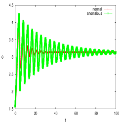
Figure 6: Comparison between $\Phi$-coupling (red line) and $z$-coupling (green line) for the phase difference when $\epsilon=\delta=1$ and $\gamma=10^{-1}$. See text for details.

In Figs. (5),(6) and (7) we plot the comparison between the population, phase differences, and the energy fluctuations calculated with the normal ($\gamma\dot{\Phi}$) and anomalous ($\gamma\dot{z}$) coupling terms for $\epsilon=1$ and $\gamma=10^{-1}$. Apart from the relaxation time and some differences in the amplitude of the oscillations, both types of coupling give place to the same equilibrium values, as expected.

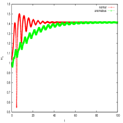
Figure 7: Comparison between $\Phi$-coupling (red line) and $z$-coupling (green line) for the energy when $\epsilon=\delta=1$ and $\gamma=10^{-1}$. See text for details.

Acknowledgement This work has been funded by the MICINN (Spain) through Grant Nos. CTQ2008-02578, FIS2010-18132, and by the Comunidad Autónoma de Madrid, Grant No. S-2009/MAT/1467. P. B. acknowledges a Juan de la Cierva fellowship from the MICINN and A.D.-U. acknowledges a JAE fellowship from CSIC. H. C. P.-R. and G. R.-L. acknowledge a scientific project from INSTEC.

References

- (1) R. A. Harris and L. Stodolsky, Phys. Lett. B 78, 313 (1978).
- (2) M. Quack, Chem. Phys. Lett. 132, 147 (1986).
- (3) U. Weiss, Quantum Dissipative Systems (2nd edn.), Series in Modern Condensed Matter Physics, World Scientific, Singapore (1999).
- (4) M. Volkhard May and O. Kühn, Charge and Energy Transfer Dynamics in Molecular Systems (2nd edn.),Wiley-VCH (2004).
- (5) M. O. Scully and M. S Zubairy, Quantum Optics, Cambridge university Press (1997).
- (6) T. D. Ladd, F. Jelezko, R. Laflamme, Y. Nakamura, C. Monroe and J. L. OBrien, Nature 464, 45 (2010).
- (7) A. J. Leggett, S. Chakravarty, A. T. Dorsey, M. P. Fisher, P. A. Matthew. A. Garg and W. Zwerger, Rev. Mod. Phys., 59, 1 (1987).
- (8) A. G. Redfield, IBM J. Res. Dev. 1, 19 (1957).
- (9) I. R Senitzki, Phys. Rev. 131, 2827 (1963).
- (10) R. A. Harris and L. Stodolsky, J. Chem. Phys. 74, 2145 (1981).
- (11) R. A. Harris and R. Silbey, J. Chem. Phys. 78, 7330 (1983).
- (12) L. Hartmann, I. Goychuk, M. Grifoni and P. Hänggi, Phys. Rev. E 61 R4687 (2000).
- (13) D. P. Vincenzo and D. Loss, Phys. Rev. B 71, 035318 (2005).
- (14) I. Gonzalo and P. Bargueño, Phys. Chem. Chem. Phys. 13, 17130 (2011)
- (15) R. Silbey and R. A. Harris, J. Chem. Phys. 80, 2615 (1984).
- (16) R. A. Harris and R. Silbey, J. Chem. Phys. 83, 1069 (1985).
- (17) R. P. Feynman, R. B. Leighton and M. Sands, Lectures on Physics vol. III, Addison–Wesley, Reading, MA (1965).
- (18) F. Strocchi, Rev. Mod. Phys. 38, 36 (1966).
- (19) A. Heslot, Phys. Rev. D 31, 1341 (1985).
- (20) H. D. Meyer and W. H. Miller, J. Chem. Phys. 70, 3214 (1979).
- (21) W. H. Miller and C. W. McCurdy, J. Chem. Phys. 69, 5163 (1978).
- (22) G. Stock and M. Thoss, Phys. Rev. Lett. 78, 578 (1997).
- (23) D. Chruszinsky and A. Jamiolkovsky, Geometric Phases in Classical and Quantum Mechanics, Progress in Mathematical Physics 36, Birkhäuser, Boston (2004).
- (24) P. Bargueño and S. Miret–Artés, Phys. Rev. A87, 012125 (2013).
- (25) H. C. Peñate–Rodríguez, P. Bargueño, G. Rojas–Lorenzo and S. Miret–Artés, J. Math. Phys., submitted.
- (26) P. Bargueño, H. C. Peñate–Rodríguez, I. Gonzalo, F. Sols and S. Miret–Artés, Chem. Phys. Lett. 516, 29 (2011).
- (27) H. C. Peñate–Rodríguez, P. Bargueño and S. Miret–Artés, Chem. Phys. Lett. 523 (2012) 49.
- (28) A. Dorta–Urra, H. C. Peñate–Rodríguez, P. Bargueño, G. Rojas–Lorenzo and S. Miret–Artés, J. Chem. Phys., 136, 174505 (2012).
- (29) H. C. Peñate–Rodríguez, A. Dorta–Urra, P. Bargueño, G. Rojas–Lorenzo and S. Miret–Artés, Chirality, 25, 514 (2013).
- (30) P. Bargueño, I. Gonzalo, R. Pérez de Tudela and S. Miret–Artés, Chem. Phys. Lett., 483, 204 (2009).
- (31) R. Görlich and U. Weiss, Phys. Rev. B 38, 5245 (1988).
- (32) P. Hänggi, G.-L. Ingold and P. Talkner, New. J. Phys. 10, 115008 (2008)
- (33) G.-L. Ingold, P. Hänggi and P. Talkner, Phys. Rev. E 79, 061105 (2009)
- (34) G.-L. Ingold, Eur. Phys. J. B 85, 30 (2012)
- (35) L. Pitaevskii and S. Stringari, Phys. Rev. Lett. 87, 180402 (2001)
- (36) I. Bengtsson and K. Zyczkowski, Geometry of Quantum States. Cambridge University Press (2006).
- (37) H.-P. Breuer and F. Petruccione, The Theory of Open Quantum Systems, Calrendon Press, Oxford, 2006
- (38) A. S. Sanz and S. Miret–Artés, A Trajectory Description of Quantum Processes. I. Fundamentals, Lecture Notes in Physics 850, Springer-Verlag (Berlin, 2012).
- (39) A. S. Sanz and S. Miret–Artés, A Trajectory Description of Quantum Processes. II. Applications, Lecture Notes in Physics XXX, Springer-Verlag (Berlin, 2013).
- (40) P. Bargueño, R. Pérez de Tudela and S. Miret–Artés and I. Gonzalo, Phys. Chem. Chem. Phys., 13, 806 (2011).
- (41) D. L. Ermak and H. Buckholtz, J. Comp. Phys., 35, 169 (1980).
- (42) M. P. Allen and D. J. Tildesley, Computer Simulation of Liquids, Oxford university Press (1987).
- (43) P. Carruthers, Rev. Mod. Phys. 40, 411 (1968)
- (44) W. H. Miller, J. Chem. Phys. 136, 210901 (2012)