Optimal Order Scheduling for Deterministic Liquidity Patterns

Peter Bank and Antje Fruth
Technische Universität Berlin
Institut für Mathematik
Straße des 17. Juni 136, 10623 Berlin, Germany
(bank@math.tu-berlin.de)
Abstract

We consider a broker who has to place a large order which consumes a sizable part of average daily trading volume. The broker’s aim is thus to minimize execution costs he incurs from the adverse impact of his trades on market prices. By contrast to the previous literature, see, e.g., Obizhaeva and Wang [7], Predoiu et al. [8], we allow the liquidity parameters of market depth and resilience to vary deterministically over the course of the trading period. The resulting singular optimal control problem is shown to be tractable by methods from convex analysis and, under minimal assumptions, we construct an explicit solution to the scheduling problem in terms of some concave envelope of the resilience adjusted market depth.

Keywords:

Order scheduling, liquidity, convexification, singular control, convex analysis, envelopes, optimal order execution

1 Introduction

It is well-known that market liquidity exhibits deterministic intraday patterns; see, e.g., Chordia et al. [3] or Kempf and Mayston [6] for some empirical investigations. The academic literature on optimal order scheduling, however, mostly considers time-invariant specifications of market depth and resilience; cf. Obizhaeva and Wang [7], Alfonsi et al. [2], Predoiu et al. [8]. It thus becomes an issue how to account for time-varying specifications of these liquidity parameters when minimizing the execution costs of a trading schedule.

Using dynamic programming techniques and calculus of variations, this problem was addressed by Fruth et al. [5]. These authors show that under certain additional assumptions on these patterns there is a time-dependent level for the ratio of the number of orders still to be scheduled and the current market impact which signals when additional orders should be placed. Explicit solutions are provided for some special cases where the broker is continually issuing orders. The thesis [4] discusses conditions under which the order signal structure persists in case of stochastically varying liquidity parameters. Acevedo and Alfonsi [1] use backward induction arguments in discrete time and then pass to continuous time to compute optimal policies for nonlinear specifications of market impacts which are scaled by a time-dependent factor satisfying some strong regularity conditions. In their approach order schedules are allowed in principle to sell and buy along the way, regardless of the sign of the desired terminal position, and they proceed to identify conditions (deemed to ensure absence of market manipulation strategies) under which optimal schedules will not do so. Optimal schedules are then obtained only under a strong assumption linking resilience and market depth to each other along with their time derivatives.

By contrast to these approaches, we focus from the outset on pure buying or selling schedules and show how to reduce our optimization problem to a convex one. Hence, we do not have to impose conditions ensuring that orders are scheduled in certain ways at certain times. Instead, optimal order sizes and times are derived endogenously from the structure of market depth and resilience alone. This is made possible by the use of convex analytic first-order characterizations of optimality which we show are intimately related to the construction of generalized concave envelopes of a resilience-adjusted form of market depth. Under minimal assumptions, this allows us to characterize when optimal schedules exist and, if so, to construct them explicitly in terms of these envelopes. We illustrate our findings by recovering the analytic solution of Obizhaeva and Wang [7] and we show how optimal schedules depend on fluctuations in market depth and the level of resilience. It turns out that with time-varying market depth optimal order schedules do not have to consist of big initial and terminal trades with infinitesimal ones in between as typically found in the previous literature. We also find that lower resilience will let optimal schedules focus more on (local) maxima of market depth to the extent that with no resilience optimal schedules trade only when market depth is at its global maximum.

2 Setup

We consider a broker who has to place an order of a total number of x>0𝑥0x>0 shares of some stock. The broker knows that, due to limited liquidity of the stock, these orders will be executed at a mark-up over some reference stock price. This mark-up will depend on the broker’s past and present trades. For our specification of the mark-up we adopt the model proposed by Obizhaeva and Wang [7], see also Alfonsi et al. [2] and Predoiu et al. [8] for further motivation of this approach. By contrast to these papers, but in line with Fruth et al. [5] and Acevedo and Alfonsi [1], we will allow for the market’s liquidity characteristics of depth and resilience to be changing over time according to a deterministic pattern.

Specifically, given the broker’s cumulative purchases X=(Xt)t0𝑋subscriptsubscript𝑋𝑡𝑡0X=(X_{t})_{t\geq 0}, a right-continuous increasing process with X00subscript𝑋limit-from00X_{0-}\triangleq 0, the resulting mark-up evolves according to the dynamics

(1) η0Xη00,dηtX=dXtδtrtηtXdtformulae-sequencesubscriptsuperscript𝜂𝑋limit-from0subscript𝜂00𝑑subscriptsuperscript𝜂𝑋𝑡𝑑subscript𝑋𝑡subscript𝛿𝑡subscript𝑟𝑡subscriptsuperscript𝜂𝑋𝑡𝑑𝑡\eta^{X}_{0-}\triangleq\eta_{0}\geq 0,\quad d\eta^{X}_{t}=\frac{dX_{t}}{\delta_{t}}-r_{t}\eta^{X}_{t}\,dt

where δtsubscript𝛿𝑡\delta_{t} describes the market’s depth at time t0𝑡0t\geq 0 and where rtsubscript𝑟𝑡r_{t} measures its current resilience. Thus, in our model market impact is taken to be a linear function of order size, the slope at any one time being determined by the market depth. Moreover, market impact decays over time at the rate specified by the market’s resilience.

Clearly, (1) has the right-continuous solution

(2) ηtX(η0+[0,t]ρsδs𝑑Xs)/ρt with ρtexp(0trs𝑑s),t0,formulae-sequencesubscriptsuperscript𝜂𝑋𝑡subscript𝜂0subscript0𝑡subscript𝜌𝑠subscript𝛿𝑠differential-dsubscript𝑋𝑠subscript𝜌𝑡 with subscript𝜌𝑡superscriptsubscript0𝑡subscript𝑟𝑠differential-d𝑠𝑡0\eta^{X}_{t}\triangleq\left(\eta_{0}+\int_{[0,t]}\frac{\rho_{s}}{\delta_{s}}\,dX_{s}\right)/\rho_{t}\text{ with }\rho_{t}\triangleq\exp\left(\int_{0}^{t}r_{s}\,ds\right),\quad t\geq 0,

under

Assumption 2.1.

The resilience pattern is given by a strictly positive and locally Lebesgue-integrable function r:[0,)(0,):𝑟00r:[0,\infty)\to(0,\infty).

In the sequel we shall require furthermore

Assumption 2.2.

The pattern of market depth δ:[0,)[0,):𝛿00\delta:[0,\infty)\to[0,\infty) is nonnegative, not identically zero, bounded and upper-semicontinuous with lim suptδt/ρt=0subscriptlimit-supremum𝑡subscript𝛿𝑡subscript𝜌𝑡0\limsup_{t\uparrow\infty}\delta_{t}/\rho_{t}=0.

The broker’s aim is to minimize the cumulative mark-up costs:

(3) MinimizeC(X)[0,)(ηtX+ΔtX2δt)𝑑Xt subject to X𝒳Minimize𝐶𝑋subscript0subscriptsuperscript𝜂𝑋limit-from𝑡subscriptΔ𝑡𝑋2subscript𝛿𝑡differential-dsubscript𝑋𝑡 subject to 𝑋𝒳\text{Minimize}\;C(X)\triangleq\int_{[0,\infty)}\left(\eta^{X}_{t-}+\frac{\Delta_{t}X}{2\delta_{t}}\right)\,dX_{t}\text{ subject to }X\in\mathcal{X}

where ΔtXXt+XtsubscriptΔ𝑡𝑋subscript𝑋limit-from𝑡subscript𝑋limit-from𝑡\Delta_{t}X\triangleq X_{t+}-X_{t-} and

𝒳{(Xt)t0 right-cont., incr. :X0=0,X=x,C(X)<}𝒳conditional-setsubscriptsubscript𝑋𝑡𝑡0 right-cont., incr. formulae-sequencesubscript𝑋limit-from00formulae-sequencesubscript𝑋𝑥𝐶𝑋\mathcal{X}\triangleq\left\{{(X_{t})_{t\geq 0}\text{ right-cont., incr. }}\;:\;X_{0-}=0,X_{\infty}=x,C(X)<\infty\right\}

with the notation XlimtXsubscript𝑋subscript𝑡𝑋X_{\infty}\triangleq\lim_{t\uparrow\infty}X.

Remark 2.3.
  1. 1.

    Note that the ΔtX2δtsubscriptΔ𝑡𝑋2subscript𝛿𝑡\frac{\Delta_{t}X}{2\delta_{t}}-term in (3) accounts for the costs a non-infinitesimal order will incur due to its own mark-up effect; cf., e.g., Alfonsi et al. [2] or Predoiu et al. [8] who in addition show how costs functionals as in (3) emerge with stochastic reference prices evolving as martingales when the broker is risk-neutral. Note also that, since we let X00subscript𝑋limit-from00X_{0-}\triangleq 0, a value of X0>0subscript𝑋00X_{0}>0 corresponds to an initial jump of size Δ0X=X0subscriptΔ0𝑋subscript𝑋0\Delta_{0}X=X_{0} in the order schedule.

  2. 2.

    To impose liquidation over a finite time horizon T0𝑇0T\geq 0, one merely has to let the market depth δt=0subscript𝛿𝑡0\delta_{t}=0 for t>T𝑡𝑇t>T. Indeed, following the convention that 1/0=101/0=\infty in the integration (2), ηXsuperscript𝜂𝑋\eta^{X} and thus the costs C(X)𝐶𝑋C(X) will then be infinite for any order schedule X𝑋X which increases after T𝑇T.

  3. 3.

    Strict positivity of r𝑟r comes without loss of generality since if resilience r=0𝑟0r=0 vanishes almost everywhere on an interval [t0,t1]subscript𝑡0subscript𝑡1[t_{0},t_{1}] there is no need to trade it off against market depth there and it is optimal to trade whatever amount is to be traded at the moment(s) when market depth δ𝛿\delta attains its maximum over this period; cf. Proposition 4.1. Hence, δ𝛿\delta could be assumed to take this maximum value at t0subscript𝑡0t_{0} and the interval (t0,t1]subscript𝑡0subscript𝑡1(t_{0},t_{1}] then be removed from consideration.

  4. 4.

    The assumption of upper-semicontinuous market depth δ𝛿\delta is necessary to rule out obvious counterexamples for existence of optimal schedules. For unbounded upper-semicontinuous δ𝛿\delta one can easily show that inf𝒳C=xη0/ρsubscriptinfimum𝒳𝐶𝑥subscript𝜂0subscript𝜌\inf_{\mathcal{X}}C=x\eta_{0}/\rho_{\infty}, and so there is no optimal schedule. The lim suplimit-supremum\limsup-condition is needed to rule out the optimality of deferring part of the order indefinitely.

  5. 5.

    Including a discount factor with locally Lebesgue-integrable discount rate r¯=(r¯t)0¯𝑟subscript¯𝑟𝑡0\bar{r}=(\bar{r}_{t})\geq 0 in our mark-up costs is equivalent to considering δ~tδtexp(0trs¯𝑑s)subscript~𝛿𝑡subscript𝛿𝑡superscriptsubscript0𝑡¯subscript𝑟𝑠differential-d𝑠\widetilde{\delta}_{t}\triangleq\delta_{t}\exp(\int_{0}^{t}\bar{r_{s}}\,ds) and r~trt+r¯tsubscript~𝑟𝑡subscript𝑟𝑡subscript¯𝑟𝑡\widetilde{r}_{t}\triangleq r_{t}+\bar{r}_{t}, t0𝑡0t\geq 0 instead of δ𝛿\delta and r𝑟r above.

3 Main result and sketch of its proof

The main result of this paper is the solution to problem (3). It describes up to what mark-up level our broker should be willing to place orders at any point in time in order to minimize mark-up costs:

Theorem 3.1.

Suppose Assumptions 2.1 and 2.2 hold, let λtδt/ρtsubscript𝜆𝑡subscript𝛿𝑡subscript𝜌𝑡\lambda_{t}\triangleq\delta_{t}/\rho_{t}, λ~tsuputλusubscript~𝜆𝑡subscriptsupremum𝑢𝑡subscript𝜆𝑢\widetilde{\lambda}_{t}\triangleq\sup_{u\geq t}\lambda_{u} and define

(4) Lt=infu>tλ~uλ~tλ~u/ρuλ~t/ρt,t0,formulae-sequencesubscriptsuperscript𝐿𝑡subscriptinfimum𝑢𝑡subscript~𝜆𝑢subscript~𝜆𝑡subscript~𝜆𝑢subscript𝜌𝑢subscript~𝜆𝑡subscript𝜌𝑡𝑡0L^{*}_{t}=\inf_{u>t}\frac{\widetilde{\lambda}_{u}-\widetilde{\lambda}_{t}}{\widetilde{\lambda}_{u}/\rho_{u}-\widetilde{\lambda}_{t}/\rho_{t}},\quad t\geq 0\,,

where we follow the convention that 0/000000/0\triangleq 0.

Then the optimal order schedule strategy is to place orders at any time t0𝑡0t\geq 0 if and while the resulting mark-up is no larger than yLt/ρtsuperscript𝑦subscriptsuperscript𝐿𝑡subscript𝜌𝑡y^{*}L^{*}_{t}/\rho_{t}, i.e.,

(5) Xt=λ0(yL0η0)++(0,t]λsdsup0vs{(yLv)η0},t0,formulae-sequencesubscriptsuperscript𝑋𝑡subscript𝜆0superscriptsuperscript𝑦subscriptsuperscript𝐿0subscript𝜂0subscript0𝑡subscript𝜆𝑠𝑑subscriptsupremum0𝑣𝑠superscript𝑦subscriptsuperscript𝐿𝑣subscript𝜂0𝑡0X^{*}_{t}=\lambda_{0}(y^{*}L^{*}_{0}-\eta_{0})^{+}+\int_{(0,t]}\lambda_{s}\,d\sup_{0\leq v\leq s}\left\{(y^{*}L^{*}_{v})\vee\eta_{0}\right\}\,,\quad t\geq 0,

provided the constant y>0superscript𝑦0y^{*}>0 in (5) can be chosen such that X=xsubscriptsuperscript𝑋𝑥X^{*}_{\infty}=x. This is the case if and only if the right side of (5) with y1superscript𝑦1y^{*}\triangleq 1 remains bounded as t𝑡t\uparrow\infty. If this is not the case, we have infX𝒳C(X)=0subscriptinfimum𝑋𝒳𝐶𝑋0\inf_{X\in\mathcal{X}}C(X)=0 and the problem does not have a solution.

The following results outline the proof of this theorem and may be of independent interest. Our first auxiliary result provides a mathematically more convenient formulation of problem (3):

Proposition 3.2.

Suppose Assumptions 2.1 and 2.2 hold, let λδ/ρ𝜆𝛿𝜌\lambda\triangleq\delta/\rho, κλ/ρ=δ/ρ2𝜅𝜆𝜌𝛿superscript𝜌2\kappa\triangleq\lambda/\rho=\delta/\rho^{2} and define, for increasing and right-continuous Y=(Yt)t0𝑌subscriptsubscript𝑌𝑡𝑡0Y=(Y_{t})_{t\geq 0},

K(Y)12[0,)κtd(Yt2).𝐾𝑌12subscript0subscript𝜅𝑡𝑑subscriptsuperscript𝑌2𝑡K(Y)\triangleq\frac{1}{2}\int_{[0,\infty)}\kappa_{t}\,d(Y^{2}_{t})\,.

Then

(6) Yt=η0+[0,t]dXsλs,Y0η0, and Xt=[0,t]λs𝑑Ys,X00,t0,formulae-sequencesubscript𝑌𝑡subscript𝜂0subscript0𝑡𝑑subscript𝑋𝑠subscript𝜆𝑠formulae-sequencesubscript𝑌limit-from0subscript𝜂0formulae-sequence and subscript𝑋𝑡subscript0𝑡subscript𝜆𝑠differential-dsubscript𝑌𝑠formulae-sequencesubscript𝑋limit-from00𝑡0Y_{t}=\eta_{0}+\int_{[0,t]}\frac{dX_{s}}{\lambda_{s}},\,Y_{0-}\triangleq\eta_{0},\text{ and }X_{t}=\int_{[0,t]}\lambda_{s}\,dY_{s},\,X_{0-}\triangleq 0,\quad t\geq 0,

define mappings from 𝒳𝒳\mathcal{X} to

𝒴{(Yt)t0 right-cont., incr. :Y0η0,[0,)λt𝑑Yt=x,K(Y)<}𝒴conditional-setsubscriptsubscript𝑌𝑡𝑡0 right-cont., incr. formulae-sequencesubscript𝑌limit-from0subscript𝜂0formulae-sequencesubscript0subscript𝜆𝑡differential-dsubscript𝑌𝑡𝑥𝐾𝑌\mathcal{Y}\triangleq\left\{{(Y_{t})_{t\geq 0}\text{ right-cont., incr. }}\;:\;Y_{0-}\triangleq\eta_{0},\int_{[0,\infty)}\lambda_{t}\,dY_{t}=x,K(Y)<\infty\right\}

and vice versa such that

C(X)=K(Y).𝐶𝑋𝐾𝑌C(X)=K(Y)\,.

As a result, with these choices of κ𝜅\kappa and λ𝜆\lambda, optimization problem (3) is equivalent to the following problem:

(7) MinimizeK(Y)12[0,)κtd(Yt2) subject to Y𝒴.Minimize𝐾𝑌12subscript0subscript𝜅𝑡𝑑subscriptsuperscript𝑌2𝑡 subject to 𝑌𝒴\text{Minimize}\;K(Y)\triangleq\frac{1}{2}\int_{[0,\infty)}\kappa_{t}\,d(Y^{2}_{t})\text{ subject to }Y\in\mathcal{Y}\,.

Neither problem (3) nor problem (7) is convex in general:

Proposition 3.3.

For upper-semicontinuous κ𝜅\kappa, the functional K=K(Y)𝐾𝐾𝑌K=K(Y) of (7) is (strictly) convex for right-continuous, increasing Y𝑌Y with Y0=η0subscript𝑌limit-from0subscript𝜂0Y_{0-}=\eta_{0} if and only if κ𝜅\kappa is (strictly) positive and (strictly) decreasing.

Convexity can always be arranged for, though, in the following sense:

Theorem 3.4.

Let λ𝜆\lambda, κ𝜅\kappa be as in Proposition 3.2. Then optimization problem (7) has the same value as the convex optimization problem

(8) MinimizeK~(Y~)12[0,)κ~td(Y~t2) subject to Y~𝒴~Minimize~𝐾~𝑌12subscript0subscript~𝜅𝑡𝑑subscriptsuperscript~𝑌2𝑡 subject to ~𝑌~𝒴\text{Minimize}\;\widetilde{K}(\widetilde{Y})\triangleq\frac{1}{2}\int_{[0,\infty)}\widetilde{\kappa}_{t}\,d(\widetilde{Y}^{2}_{t})\text{ subject to }\widetilde{Y}\in\widetilde{\mathcal{Y}}

where κ~tλ~t/ρtsubscript~𝜅𝑡subscript~𝜆𝑡subscript𝜌𝑡\widetilde{\kappa}_{t}\triangleq\widetilde{\lambda}_{t}/\rho_{t}, λ~tsuputλusubscript~𝜆𝑡subscriptsupremum𝑢𝑡subscript𝜆𝑢\widetilde{\lambda}_{t}\triangleq\sup_{u\geq t}\lambda_{u}, t0𝑡0t\geq 0, and

𝒴~{(Y~t)t0 right-cont., incr. :Y~0η0,[0,)λ~t𝑑Y~t=x,K~(Y~)<}.~𝒴conditional-setsubscriptsubscript~𝑌𝑡𝑡0 right-cont., incr. formulae-sequencesubscript~𝑌limit-from0subscript𝜂0formulae-sequencesubscript0subscript~𝜆𝑡differential-dsubscript~𝑌𝑡𝑥~𝐾~𝑌\widetilde{\mathcal{Y}}\triangleq\left\{{(\widetilde{Y}_{t})_{t\geq 0}\text{ right-cont., incr. }}\;:\;\widetilde{Y}_{0-}\triangleq\eta_{0},\int_{[0,\infty)}\widetilde{\lambda}_{t}\,d\widetilde{Y}_{t}=x,\widetilde{K}(\widetilde{Y})<\infty\right\}\,.

Moreover, any solution Y~superscript~𝑌\widetilde{Y}^{*} to (8) with {dY~>0}{λ~=λ}𝑑superscript~𝑌0~𝜆𝜆\{d\widetilde{Y}^{*}>0\}\subset\{\widetilde{\lambda}=\lambda\} will also be a solution to (7).

Remark 3.5.

For an increasing process Y=(Yt)t0𝑌subscriptsubscript𝑌𝑡𝑡0Y=(Y_{t})_{t\geq 0} we say that t𝑡t is a point of increase towards the right and write dYt>0𝑑subscript𝑌𝑡0dY_{t}>0 if Yt<Yusubscript𝑌limit-from𝑡subscript𝑌𝑢Y_{t-}<Y_{u} for any u>t𝑢𝑡u>t. A similar convention applies to decreasing processes and points of decrease towards the right.

The next proposition describes the (necessary and sufficient) first-order conditions for optimality in problem (8). As one would expect, the broker has to strike a balance between the impact of current orders on future mark-up costs (as represented by the left side of (9) below) and the current prospect on future market conditions (as represented by the decreasing envelope λ~~𝜆\widetilde{\lambda} of market depth over resilience on the right side of that equation):

Proposition 3.6.

For κ~~𝜅\widetilde{\kappa}, λ~0~𝜆0\widetilde{\lambda}\geq 0 as in Theorem 3.4, Y~𝒴~superscript~𝑌~𝒴\widetilde{Y}^{*}\in\widetilde{\mathcal{Y}} solves (8) if and only if there is a constant y>0𝑦0y>0 such that

(9) [t,)Y~u𝑑κ~uyλ~t for t0 with ‘=’ whenever dY~t>0.subscript𝑡subscriptsuperscript~𝑌𝑢differential-dsubscript~𝜅𝑢𝑦subscript~𝜆𝑡 for t0 with ‘=’ whenever 𝑑subscriptsuperscript~𝑌𝑡0-\int_{[t,\infty)}\widetilde{Y}^{*}_{u}\,d\widetilde{\kappa}_{u}\geq y\widetilde{\lambda}_{t}\text{ for $t\geq 0$ with `$=$' whenever }d\widetilde{Y}^{*}_{t}>0\,.

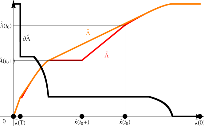
Constructing right-continuous increasing Y~0superscript~𝑌0\widetilde{Y}^{*}\geq 0 satisfying the first order conditions of (9) can be done by using a time-change and concave envelopes; see also Figure 3 below:

Theorem 3.7.

Under Assumptions 2.1 and 2.2, consider the level passage times τkinf{t0:κ~tk}subscript𝜏𝑘infimumconditional-set𝑡0subscript~𝜅𝑡𝑘{\tau}_{k}\triangleq\inf\left\{{t\geq 0}\;:\;\widetilde{\kappa}_{t}\leq k\right\} and let Λ~kkρτksubscript~Λ𝑘𝑘subscript𝜌subscript𝜏𝑘\widetilde{\Lambda}_{k}\triangleq k\rho_{\tau_{k}}, k(0,κ~0]𝑘0subscript~𝜅0k\in(0,\widetilde{\kappa}_{0}] and Λ~00subscript~Λ00\widetilde{\Lambda}_{0}\triangleq 0.

Then Λ~~Λ\widetilde{\Lambda} is a continuous increasing map on [0,κ~0]0subscript~𝜅0[0,\widetilde{\kappa}_{0}]. Its concave envelope Λ^^Λ\widehat{{\Lambda}} is absolutely continuous with a left-continuous, decreasing density Λ^=(Λ^k)0<kκ~00^Λsubscriptsubscript^Λ𝑘0𝑘subscript~𝜅00\partial\widehat{{\Lambda}}=(\partial\widehat{\Lambda}_{k})_{0<k\leq\widetilde{\kappa}_{0}}\geq 0. Moreover, letting Λ^0Λ^0+subscript^Λ0subscript^Λlimit-from0\partial\widehat{{\Lambda}}_{0}\triangleq\partial\widehat{{\Lambda}}_{0+}, we have that for any y>0𝑦0y>0 and η00subscript𝜂00\eta_{0}\geq 0, Y~t(yΛ^κ~t)η0subscriptsuperscript~𝑌𝑡𝑦subscript^Λsubscript~𝜅𝑡subscript𝜂0\widetilde{Y}^{*}_{t}\triangleq(y\partial\widehat{{\Lambda}}_{\widetilde{\kappa}_{t}})\vee\eta_{0}, t0𝑡0t\geq 0, with Y~0η0subscriptsuperscript~𝑌limit-from0subscript𝜂0\widetilde{Y}^{*}_{0-}\triangleq\eta_{0} yields a right-continuous increasing process satisfying (9).

Combining the previous results, we shall obtain the following solution to our original problem (3) which also provides a characterization different from that outlined in Theorem 3.1; see also Figure 2 below:

Corollary 3.8.

Under the assumptions of Theorem 3.7 and using its notation we have the following dichotomy:

In case |Λ^|𝐋2(0κ~0(Λ^k)2𝑑k)12<subscript^Λsuperscript𝐋2superscriptsuperscriptsubscript0subscript~𝜅0superscriptsubscript^Λ𝑘2differential-d𝑘12|\partial\widehat{\Lambda}|_{\mathbf{L}^{2}}\triangleq(\int_{0}^{\widetilde{\kappa}_{0}}(\partial\widehat{\Lambda}_{k})^{2}\,dk)^{\frac{1}{2}}<\infty we can choose y>0superscript𝑦0y^{*}>0 uniquely such that

(10) Xtλ0(yΛ^κ~0η0)++(0,t]λsd{(yΛ^κ~s)η0},t0,formulae-sequencesubscriptsuperscript𝑋𝑡subscript𝜆0superscriptsuperscript𝑦subscript^Λsubscript~𝜅0subscript𝜂0subscript0𝑡subscript𝜆𝑠𝑑superscript𝑦subscript^Λsubscript~𝜅𝑠subscript𝜂0𝑡0X^{*}_{t}\triangleq\lambda_{0}(y^{*}\partial\widehat{\Lambda}_{\widetilde{\kappa}_{0}}-\eta_{0})^{+}+\int_{(0,t]}\lambda_{s}\,d\left\{(y^{*}\partial\widehat{\Lambda}_{\widetilde{\kappa}_{s}})\vee\eta_{0}\right\},\quad t\geq 0,

increases from X00subscriptsuperscript𝑋limit-from00X^{*}_{0-}\triangleq 0 to X=xsubscriptsuperscript𝑋𝑥X^{*}_{\infty}=x; this X𝒳superscript𝑋𝒳X^{*}\in\mathcal{X} is an optimal order schedule for problem (3). In the special case where η0=0subscript𝜂00\eta_{0}=0, y=x/|Λ^|𝐋22superscript𝑦𝑥superscriptsubscript^Λsuperscript𝐋22y^{*}=x/|\partial\widehat{\Lambda}|_{\mathbf{L}^{2}}^{2} and the minimal costs are given by C(X)=x2/(2|Λ^|𝐋22)𝐶superscript𝑋superscript𝑥22superscriptsubscript^Λsuperscript𝐋22C(X^{*})=x^{2}/(2|\partial\widehat{\Lambda}|_{\mathbf{L}^{2}}^{2}).

If, by contrast, |Λ^|𝐋2=subscript^Λsuperscript𝐋2|\partial\widehat{\Lambda}|_{\mathbf{L}^{2}}=\infty then we have infX𝒳C(X)=0subscriptinfimum𝑋𝒳𝐶𝑋0\inf_{X\in\mathcal{X}}C(X)=0 and problem (3) does not have a solution.

4 Illustrations

Corollary 3.8 reduces the construction of optimal order schedules to the computation of a concave envelope. This can often be done in closed form, see, e.g., our treatment in Section 4.1 of the constant parameter case from Obizhaeva and Wang [7]. Alternatively, one can resort to highly efficient numerical methods from discrete geometry to come up with solutions to essentially arbitrary liquidity patterns as we illustrate in Section 4.2.

4.1 Constant market depth and resilience

Let us first show how to recover the solution of Obizhaeva and Wang [7] who consider a time horizon T>0𝑇0T>0 and constant market depth δtδ01[0,T](t)subscript𝛿𝑡subscript𝛿0subscript10𝑇𝑡\delta_{t}\equiv\delta_{0}1_{[0,T]}(t) and constant market resilience rtr0>0subscript𝑟𝑡subscript𝑟00r_{t}\equiv r_{0}>0, t0𝑡0t\geq 0. In this case we have

λtsubscript𝜆𝑡\displaystyle\lambda_{t} =λ~t=δ0er0t1[0,T](t) and κt=κ~t=δ0e2r0t1[0,T](t).absentsubscript~𝜆𝑡subscript𝛿0superscript𝑒subscript𝑟0𝑡subscript10𝑇𝑡 and subscript𝜅𝑡subscript~𝜅𝑡subscript𝛿0superscript𝑒2subscript𝑟0𝑡subscript10𝑇𝑡\displaystyle=\widetilde{\lambda}_{t}=\delta_{0}e^{-r_{0}t}1_{[0,T]}(t)\text{ and }\kappa_{t}=\widetilde{\kappa}_{t}=\delta_{0}e^{-2r_{0}t}1_{[0,T]}(t)\,.

Hence,

ρτk=δ0/(kκT) and Λ~k=δ0k(δ0/κTk),0kδ0.formulae-sequencesubscript𝜌subscript𝜏𝑘subscript𝛿0𝑘subscript𝜅𝑇 and subscript~Λ𝑘subscript𝛿0𝑘subscript𝛿0subscript𝜅𝑇𝑘0𝑘subscript𝛿0\displaystyle\rho_{\tau_{k}}=\sqrt{\delta_{0}/(k\vee\kappa_{T})}\text{ and }\widetilde{\Lambda}_{k}=\sqrt{\delta_{0}k}\wedge(\sqrt{\delta_{0}/\kappa_{T}}k),\quad 0\leq k\leq\delta_{0}.

Thus, Λ~~Λ\widetilde{\Lambda} is its own concave envelope, i.e., Λ~=Λ^~Λ^Λ\widetilde{\Lambda}=\widehat{\Lambda}, and its left-continuous density is

Λ^k={12δ0/k,k>κT,δ0/κT=er0T,kκT.subscript^Λ𝑘cases12subscript𝛿0𝑘𝑘subscript𝜅𝑇subscript𝛿0subscript𝜅𝑇superscript𝑒subscript𝑟0𝑇𝑘subscript𝜅𝑇\partial\widehat{\Lambda}_{k}=\begin{cases}\frac{1}{2}\sqrt{{\delta_{0}}/{k}},\quad&k>\kappa_{T},\\ \sqrt{\delta_{0}/\kappa_{T}}=e^{r_{0}T},\quad&k\leq\kappa_{T}.\end{cases}

Obviously Λ^^Λ\partial\widehat{\Lambda} is square integrable (and hence the problem is well-posed) if and only if T<𝑇T<\infty. In that case, we compute

Y^tΛ^κ~t={12δ0/κt=12er0t,t<T,δ0/κT=er0T,tT,subscript^𝑌𝑡subscript^Λsubscript~𝜅𝑡cases12subscript𝛿0subscript𝜅𝑡12superscript𝑒subscript𝑟0𝑡𝑡𝑇subscript𝛿0subscript𝜅𝑇superscript𝑒subscript𝑟0𝑇𝑡𝑇\widehat{Y}_{t}\triangleq\partial\widehat{\Lambda}_{\widetilde{\kappa}_{t}}=\begin{cases}\frac{1}{2}\sqrt{\delta_{0}/\kappa_{t}}=\frac{1}{2}e^{r_{0}t},\quad&t<T,\\ \sqrt{\delta_{0}/\kappa_{T}}=e^{r_{0}T},\quad&t\geq T,\end{cases}

and for any y>0𝑦0y>0 the order schedule from (10),

Xtyδ0(12yη0)++12yδ0r0(tTτy)++12δ0y1[T,](t),t0,formulae-sequencesubscriptsuperscript𝑋𝑦𝑡subscript𝛿0superscript12𝑦subscript𝜂012𝑦subscript𝛿0subscript𝑟0superscript𝑡𝑇superscript𝜏𝑦12subscript𝛿0𝑦subscript1𝑇𝑡𝑡0X^{y}_{t}\triangleq\delta_{0}\left(\frac{1}{2}y-\eta_{0}\right)^{+}+\frac{1}{2}y\delta_{0}r_{0}\left(t\wedge T-\tau^{y}\right)^{+}+\frac{1}{2}\delta_{0}y1_{[T,\infty]}(t),\quad t\geq 0,

with

τy{(1r0log2η0y)+T,y>2η0er0T,T,η0er0Ty2η0er0T,y<η0er0T,superscript𝜏𝑦casessuperscript1subscript𝑟02subscript𝜂0𝑦𝑇𝑦2subscript𝜂0superscript𝑒subscript𝑟0𝑇𝑇subscript𝜂0superscript𝑒subscript𝑟0𝑇𝑦2subscript𝜂0superscript𝑒subscript𝑟0𝑇𝑦subscript𝜂0superscript𝑒subscript𝑟0𝑇\tau^{y}\triangleq\begin{cases}\left(\frac{1}{r_{0}}\log\frac{2\eta_{0}}{y}\right)^{+}\wedge T,&y>2\eta_{0}e^{-r_{0}T},\\ T,&\eta_{0}e^{-r_{0}T}\leq y\leq 2\eta_{0}e^{-r_{0}T},\\ \infty&y<\eta_{0}e^{-r_{0}T},\end{cases}

is optimal for the total volume it trades. In particular, if η0=0subscript𝜂00\eta_{0}=0, we find that

Xty=yδ02(1+r0(tT)+1[T,](t)),t0.formulae-sequencesubscriptsuperscript𝑋𝑦𝑡𝑦subscript𝛿021subscript𝑟0𝑡𝑇subscript1𝑇𝑡𝑡0X^{y}_{t}=\frac{y\delta_{0}}{2}\left(1+r_{0}(t\wedge T)+1_{[T,\infty]}(t)\right),\quad t\geq 0.

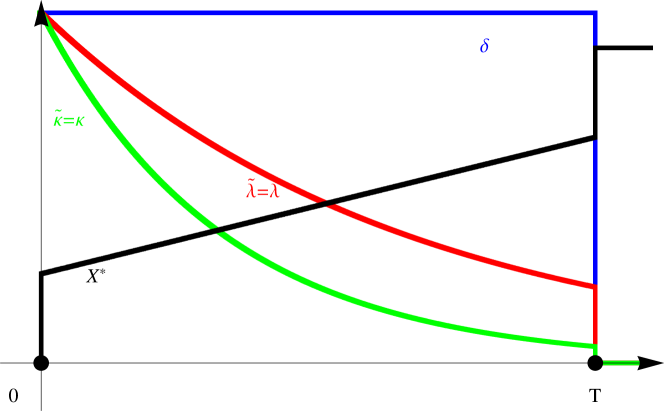
So choosing yx/(δ0(1+r0T/2))superscript𝑦𝑥subscript𝛿01subscript𝑟0𝑇2y^{*}\triangleq x/(\delta_{0}(1+r_{0}T/2)) yields X=Xysuperscript𝑋superscript𝑋superscript𝑦X^{*}=X^{y^{*}} with X=xsubscriptsuperscript𝑋𝑥X^{*}_{\infty}=x. We therefore recover the result of Obizhaeva and Wang [7]: If η0=0subscript𝜂00\eta_{0}=0, i.e., if there have been no previous orders, it is optimal to place orders of size yδ0/2superscript𝑦subscript𝛿02y^{*}\delta_{0}/2 at both t=0𝑡0t=0 and t=T𝑡𝑇t=T, and to place orders at the constant rate yδ0r0/2superscript𝑦subscript𝛿0subscript𝑟02y^{*}\delta_{0}r_{0}/2 in between; cf. Figure 1.

Refer to caption
Figure 1: Optimal order schedule Xsuperscript𝑋X^{*} (black) for constant market depth δ𝛿\delta (blue), its resilience adjustment λ=λ~𝜆~𝜆\lambda=\widetilde{\lambda} (red), κ=κ~𝜅~𝜅\kappa=\widetilde{\kappa} (green) over a finite horizon T𝑇T.

4.2 Time-varying market depth

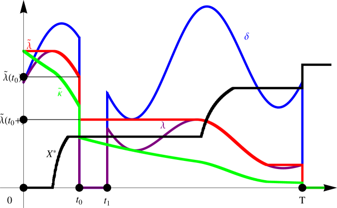
We next illustrate that the above order placement strategy of [7] is indeed strongly dependent on constant market depth and resilience. Figure 2 below exhibits how a fluctuating market depth affects the timing of the optimal order placement as provided by Corollary 3.8. Note that we include a shut-down period for the market over the time period (t0,t1)subscript𝑡0subscript𝑡1(t_{0},t_{1}) when market depth vanishes. The corresponding concepts introduced by Theorem 3.7 are illustrated in Figure 3 below.
Refer to caption
Figure 2: A specification of market depth δ𝛿\delta (blue) with finite horizon T𝑇T, its resilience adjustment λ𝜆\lambda (purple), the corresponding decreasing envelope λ~~𝜆\widetilde{\lambda} (red) and κ~~𝜅\widetilde{\kappa} (green) along with an optimal order schedule Xsuperscript𝑋X^{*} (black).
Refer to caption
Figure 3: The decreasing envelope of resilience adjusted market depth Λ~~Λ\widetilde{\Lambda} (red), its concave envelope Λ^^Λ\widehat{\Lambda} (orange) and the density Λ^^Λ\partial\widehat{\Lambda} (black).

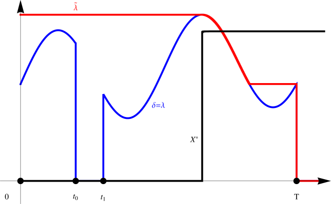
If we decrease the resilience parameter to r0=0subscript𝑟00r_{0}=0, i.e., we assume permament price impact of the broker’s orders, the focus on peaks of market depth sharpens to the extent that eventually only one huge order is placed when market depth reaches its global maximum; see Figure 4.
Refer to caption
Figure 4: Optimal order schedule Xsuperscript𝑋X^{*} (black) without market resilience and time-varying market depth δ𝛿\delta (blue).
Proposition 4.1.

If r0𝑟0r\equiv 0 and δ𝛿\delta satisfies Assumption 2.2, the solutions to optimization problem (3) are precisely those order schedules X𝒳superscript𝑋𝒳X^{*}\in\mathcal{X} with {dX>0}argmaxδ𝑑superscript𝑋0argmax𝛿\{dX^{*}>0\}\subset\operatorname*{arg\>max}\delta.

Proof.

When r0𝑟0r\equiv 0, ρ1𝜌1\rho\equiv 1 and so ηtX=η0+[0,t]dXsδsη0+Xtmaxδsubscriptsuperscript𝜂𝑋𝑡subscript𝜂0subscript0𝑡𝑑subscript𝑋𝑠subscript𝛿𝑠subscript𝜂0subscript𝑋𝑡𝛿\eta^{X}_{t}=\eta_{0}+\int_{[0,t]}\frac{dX_{s}}{\delta_{s}}\geq\eta_{0}+\frac{X_{t}}{\max\delta}, t0𝑡0t\geq 0. Thus,

C(X)η0x+x22maxδ,X𝒳,formulae-sequence𝐶𝑋subscript𝜂0𝑥superscript𝑥22𝛿𝑋𝒳C(X)\geq\eta_{0}x+\frac{x^{2}}{2\max\delta},\quad X\in\mathcal{X},

with equality for all X𝒳superscript𝑋𝒳X^{*}\in\mathcal{X} with {dX>0}argmaxδ𝑑superscript𝑋0argmax𝛿\{dX^{*}>0\}\subset\operatorname*{arg\>max}\delta. ∎

Conversely, with high resilience, orders tend to be spread out more around local maxima of market depth as illustrated by Figure 5. Figures 2 and 5 also show that the precise moments when it is optimal to issue orders would be hard to guess in advance. Hence, an approach via classical calculus of variations as in Fruth et al. [5] or via the methods of Acevedo and Alfonsi [1] seems infeasible in these general cases.
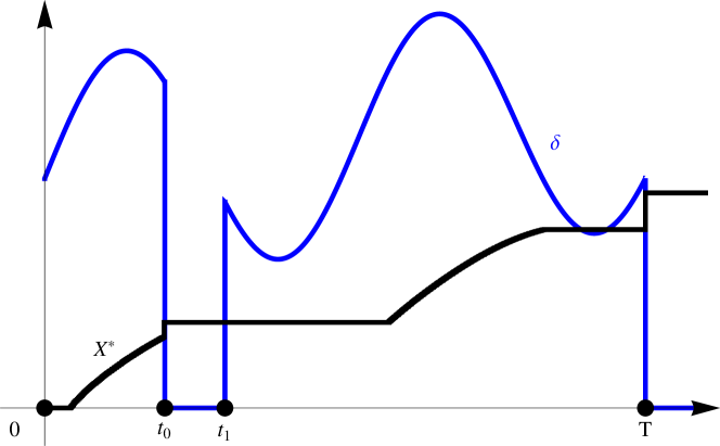
Refer to caption
Figure 5: Optimal order schedule Xsuperscript𝑋X^{*} (black) with strong market resilience for time-varying market depth δ𝛿\delta (blue).

5 Proofs

We first prove that the original problem (3) can indeed be reformulated as (7) by giving the

Proof of Proposition 3.2 We first observe that for X𝒳𝑋𝒳X\in\mathcal{X} the mapping in (6) defines an increasing right-continuous Y𝑌Y with Y=ρηX𝑌𝜌superscript𝜂𝑋Y=\rho\eta^{X}. Because C(X)<𝐶𝑋C(X)<\infty, ηXsuperscript𝜂𝑋\eta^{X} is dX𝑑𝑋dX-integrable and thus finite on {X<x}𝑋𝑥\{X<x\}. Hence, Y𝑌Y is finite on this set as well and we conclude dX=λdY𝑑𝑋𝜆𝑑𝑌dX=\lambda\,dY. It follows by elementary calculus that K(Y)=C(X)𝐾𝑌𝐶𝑋K(Y)=C(X) and, thus, Y𝒴𝑌𝒴Y\in\mathcal{Y} as desired.

Conversely, for Y𝒴𝑌𝒴Y\in\mathcal{Y}, κ=λ/ρ𝜅𝜆𝜌\kappa=\lambda/\rho is d(Y2)𝑑superscript𝑌2d(Y^{2})-integrable. Since ρ>0𝜌0\rho>0 is continuous this implies that λ𝜆\lambda is locally dY𝑑𝑌dY-integrable and so X𝑋X given by (6) is right-continuous and increasing with dX=λdY𝑑𝑋𝜆𝑑𝑌dX=\lambda\,dY. By the same reasoning as above this implies C(X)=K(Y)𝐶𝑋𝐾𝑌C(X)=K(Y) as well as X𝒳𝑋𝒳X\in\mathcal{X}. ∎

We next characterize when problem (7) is convex:

Proof of Proposition 3.3 If κ𝜅\kappa is upper semi-continuous and decreasing, it is also left-continuous and we can use Fubini’s theorem to write

K(Y)=12(κ(Y2η02)[0,)(Yt2η02)𝑑κt)𝐾𝑌12subscript𝜅subscriptsuperscript𝑌2superscriptsubscript𝜂02subscript0subscriptsuperscript𝑌2𝑡superscriptsubscript𝜂02differential-dsubscript𝜅𝑡K(Y)=\frac{1}{2}\left(\kappa_{\infty}(Y^{2}_{\infty}-\eta_{0}^{2})-\int_{[0,\infty)}(Y^{2}_{t}-\eta_{0}^{2})\,d\kappa_{t}\right)

for any right-continuous increasing Y𝑌Y with Y0=η0subscript𝑌limit-from0subscript𝜂0Y_{0-}=\eta_{0}. Hence, K=K(Y)𝐾𝐾𝑌K=K(Y) is obviously convex in such Y𝑌Y with strict convexity holding true on its domain for strictly decreasing κ𝜅\kappa.

Conversely, consider for 0s<t<0𝑠𝑡0\leq s<t<\infty the function Yη0+a1[s,]+b1[t,]𝑌subscript𝜂0𝑎subscript1𝑠𝑏subscript1𝑡Y\triangleq\eta_{0}+a1_{[s,\infty]}+b1_{[t,\infty]}. Then

K(Y)𝐾𝑌\displaystyle K(Y) =12(κs((a+η0)2η02)+κt((a+b+η0)2(a+η02)))absent12subscript𝜅𝑠superscript𝑎subscript𝜂02superscriptsubscript𝜂02subscript𝜅𝑡superscript𝑎𝑏subscript𝜂02𝑎superscriptsubscript𝜂02\displaystyle=\frac{1}{2}\left(\kappa_{s}((a+\eta_{0})^{2}-\eta_{0}^{2})+\kappa_{t}\left((a+b+\eta_{0})^{2}-(a+\eta_{0}^{2})\right)\right)
=12κsa2+κtab+12κtb2+η0(aκs+bκt)absent12subscript𝜅𝑠superscript𝑎2subscript𝜅𝑡𝑎𝑏12subscript𝜅𝑡superscript𝑏2subscript𝜂0𝑎subscript𝜅𝑠𝑏subscript𝜅𝑡\displaystyle=\frac{1}{2}\kappa_{s}a^{2}+\kappa_{t}ab+\frac{1}{2}\kappa_{t}b^{2}+\eta_{0}(a\kappa_{s}+b\kappa_{t})

is convex in a,b>0𝑎𝑏0a,b>0 if and only if κsκt0subscript𝜅𝑠subscript𝜅𝑡0\kappa_{s}\geq\kappa_{t}\geq 0, with strict inequalities corresponding to strict convexity. ∎

In order to prepare the proof of Theorem 3.4 let us recall that for any increasing Z:[0,)𝐑:𝑍0𝐑Z:[0,\infty)\to\mathbf{R} we let

{dZ>0}{t0:Zt<Zufor allu>t}𝑑𝑍0conditional-set𝑡0formulae-sequencesubscript𝑍limit-from𝑡subscript𝑍𝑢for all𝑢𝑡\{dZ>0\}\triangleq\left\{{t\geq 0}\;:\;Z_{t-}<Z_{u}\quad\text{for all}\quad u>t\right\}

denote the collection of all points of increase towards the right. For a decreasing Z𝑍Z we let {dZ<0}{d(Z)>0}𝑑𝑍0𝑑𝑍0\{dZ<0\}\triangleq\{d(-Z)>0\}. In either case we let suppdZsupp𝑑𝑍\operatorname{\mathrm{supp}}dZ denote the support of the measure dZ𝑑𝑍dZ, i.e., the smallest closed set whose complement has vanishing dZ𝑑𝑍dZ-measure.

Lemma 5.1.

For upper-semicontinuous, bounded λ:[0,)𝐑:𝜆0𝐑\lambda:[0,\infty)\to\mathbf{R}, we have that λ~tsuputλusubscript~𝜆𝑡subscriptsupremum𝑢𝑡subscript𝜆𝑢\widetilde{\lambda}_{t}\triangleq\sup_{u\geq t}\lambda_{u} is left-continuous and decreasing with

(11) {dλ~<0}{λ~=λ}.𝑑~𝜆0~𝜆𝜆\{d\widetilde{\lambda}<0\}\subset\{\widetilde{\lambda}=\lambda\}\,.

Moreover, we have the partition

(12) 𝐑={dλ~<0}nN1[ln,rn)nN2(ln,rn)𝐑𝑑~𝜆0subscript𝑛subscript𝑁1subscript𝑙𝑛subscript𝑟𝑛subscript𝑛subscript𝑁2subscript𝑙𝑛subscript𝑟𝑛\mathbf{R}=\{d\widetilde{\lambda}<0\}\cup\bigcup_{n\in N_{1}}[l_{n},r_{n})\cup\bigcup_{n\in N_{2}}(l_{n},r_{n})

where (ln,rn)subscript𝑙𝑛subscript𝑟𝑛(l_{n},r_{n}), nN𝑛𝑁n\in N, are the disjoint open intervals forming 𝐑\suppdλ~\𝐑supp𝑑~𝜆\mathbf{R}\backslash\operatorname{\mathrm{supp}}d\widetilde{\lambda} and where N1={nN:ln0,Δlnλ~=0}subscript𝑁1conditional-set𝑛𝑁formulae-sequencesubscript𝑙𝑛0subscriptΔsubscript𝑙𝑛~𝜆0N_{1}=\left\{{n\in N}\;:\;l_{n}\geq 0,\Delta_{l_{n}}\widetilde{\lambda}=0\right\} and N2=N\N1subscript𝑁2\𝑁subscript𝑁1N_{2}=N\backslash N_{1}.

Proof.

Left-continuity of λ~~𝜆\widetilde{\lambda} and relation (11) are immediate. Note next that {dλ~<0}suppdλ~𝑑~𝜆0supp𝑑~𝜆\{d\widetilde{\lambda}<0\}\subset\operatorname{\mathrm{supp}}d\widetilde{\lambda} and therefore 𝐑\{dλ~<0}nN(ln,rn)subscript𝑛𝑁subscript𝑙𝑛subscript𝑟𝑛\𝐑𝑑~𝜆0\mathbf{R}\backslash\{d\widetilde{\lambda}<0\}\supset\bigcup_{n\in N}(l_{n},r_{n}). Hence, to deduce partition (12) it suffices to observe that for nN1𝑛subscript𝑁1n\in N_{1} we have ln{dλ~<0}subscript𝑙𝑛𝑑~𝜆0l_{n}\not\in\{d\widetilde{\lambda}<0\} and that for t0𝑡0t\geq 0 such that λ~t=λ~usubscript~𝜆𝑡subscript~𝜆𝑢\widetilde{\lambda}_{t}=\widetilde{\lambda}_{u} for some u>t𝑢𝑡u>t we have (t,u)(ln,rn)𝑡𝑢subscript𝑙𝑛subscript𝑟𝑛(t,u)\subset(l_{n},r_{n}) for some nN𝑛𝑁n\in N, and thus t(ln,rn)𝑡subscript𝑙𝑛subscript𝑟𝑛t\in(l_{n},r_{n}) or t=ln𝑡subscript𝑙𝑛t=l_{n} with Δlnλ~=0subscriptΔsubscript𝑙𝑛~𝜆0\Delta_{l_{n}}\widetilde{\lambda}=0. ∎

The main tool in the proof of Theorem 3.4 is the following

Lemma 5.2.

Under the conditions of Theorem 3.4, we can find for any increasing, right-continuous Yη0𝑌subscript𝜂0Y\geq\eta_{0} an increasing, right-continuous Y~η0~𝑌subscript𝜂0\widetilde{Y}\geq\eta_{0} such that Y~Y~𝑌𝑌\widetilde{Y}\leq Y and

  • (i)

    [0,)λt𝑑Yt=[0,)λt𝑑Y~tsubscript0subscript𝜆𝑡differential-dsubscript𝑌𝑡subscript0subscript𝜆𝑡differential-dsubscript~𝑌𝑡\int_{[0,\infty)}\lambda_{t}\,dY_{t}=\int_{[0,\infty)}\lambda_{t}\,d\widetilde{Y}_{t},

  • (ii)

    {dY~>0}{dλ~<0}𝑑~𝑌0𝑑~𝜆0\{d\widetilde{Y}>0\}\subset\{d\widetilde{\lambda}<0\},

  • (iii)

    K(Y)K(Y~)=K~(Y~)𝐾𝑌𝐾~𝑌~𝐾~𝑌K(Y)\geq K(\widetilde{Y})=\widetilde{K}(\widetilde{Y}).

Proof.

We let Insubscript𝐼𝑛I_{n}, nN𝑛𝑁n\in N, denote the disjoint intervals of Lemma 5.1 forming the complement of {dλ~<0}𝑑~𝜆0\{d\widetilde{\lambda}<0\} and we will use lnsubscript𝑙𝑛l_{n}, rnsubscript𝑟𝑛r_{n} to denote their respective boundaries. For the one interval Insubscript𝐼𝑛I_{n} whose left bound is ln=subscript𝑙𝑛l_{n}=-\infty we now redefine, for simplicity of notation, ln0subscript𝑙𝑛0l_{n}\triangleq 0 provided that rn>0subscript𝑟𝑛0r_{n}>0; if, by contrast, this Insubscript𝐼𝑛I_{n} is just the negative half line we can and shall remove it from consideration in the sequel. Similarly, if rn=subscript𝑟𝑛r_{n}=\infty for some nN𝑛𝑁n\in N, it follows from Assumption 2.2 that δt=λt=κt0subscript𝛿𝑡subscript𝜆𝑡subscript𝜅𝑡0\delta_{t}=\lambda_{t}=\kappa_{t}\equiv 0 on Insubscript𝐼𝑛I_{n} which thus can be disregarded as well.

Observe then that

(13) supInλ=λrn,subscriptsupremumsubscript𝐼𝑛𝜆subscript𝜆subscript𝑟𝑛\sup_{I_{n}}\lambda=\lambda_{r_{n}}\,,

by upper semi-continuity of λ𝜆\lambda and our choice when to include lnsubscript𝑙𝑛l_{n} in Insubscript𝐼𝑛I_{n} and when not.

Let, for t0𝑡0t\geq 0,

Y~tη0subscript~𝑌𝑡subscript𝜂0\displaystyle\widetilde{Y}_{t}\triangleq\eta_{0} +[0,t]1{dλ~<0}(s)𝑑Ys+nN,rntInλsλrn𝑑Ys.subscript0𝑡subscript1𝑑~𝜆0𝑠differential-dsubscript𝑌𝑠subscriptformulae-sequence𝑛𝑁subscript𝑟𝑛𝑡subscriptsubscript𝐼𝑛subscript𝜆𝑠subscript𝜆subscript𝑟𝑛differential-dsubscript𝑌𝑠\displaystyle+\int_{[0,t]}1_{\{d\widetilde{\lambda}<0\}}(s)\,dY_{s}+\sum_{n\in N,r_{n}\leq t}\int_{I_{n}}\frac{\lambda_{s}}{\lambda_{r_{n}}}\,dY_{s}\,.

We first note that Y~Y~𝑌𝑌\widetilde{Y}\leq Y. Indeed

YtY~t=subscript𝑌𝑡subscript~𝑌𝑡absent\displaystyle Y_{t}-\widetilde{Y}_{t}= [0,t]1𝐑\{dλ~<0}(s)(dYsdY~s)subscript0𝑡subscript1\𝐑𝑑~𝜆0𝑠𝑑subscript𝑌𝑠𝑑subscript~𝑌𝑠\displaystyle\int_{[0,t]}1_{\mathbf{R}\backslash\{d\widetilde{\lambda}<0\}}(s)\,(dY_{s}-d\widetilde{Y}_{s})
=\displaystyle= nN,lnt(In[0,t]𝑑Ys1[rn,)(t)Inλsλrn𝑑Ys)subscriptformulae-sequence𝑛𝑁subscript𝑙𝑛𝑡subscriptsubscript𝐼𝑛0𝑡differential-dsubscript𝑌𝑠subscript1subscript𝑟𝑛𝑡subscriptsubscript𝐼𝑛subscript𝜆𝑠subscript𝜆subscript𝑟𝑛differential-dsubscript𝑌𝑠\displaystyle\sum_{n\in N,l_{n}\leq t}\left(\int_{I_{n}\cap[0,t]}\,dY_{s}-1_{[r_{n},\infty)}(t)\int_{I_{n}}\frac{\lambda_{s}}{\lambda_{r_{n}}}\,dY_{s}\right)

is nonnegative because of (13).

Assertion (i) is readily checked using the partition given by (12). For assertion (ii) it suffices to observe that all rnsubscript𝑟𝑛r_{n}, nN𝑛𝑁n\in N, are contained in {dλ~<0}𝑑~𝜆0\{d\widetilde{\lambda}<0\}.

In order to prove assertion (iii), we first note that K(Y~)=K~(Y~)𝐾~𝑌~𝐾~𝑌K(\widetilde{Y})=\widetilde{K}(\widetilde{Y}) is an immediate consequence of (ii) and (11). To establish K(Y)K(Y~)0𝐾𝑌𝐾~𝑌0K(Y)-K(\widetilde{Y})\geq 0 we decompose this difference into its contributions from the different parts in the partition given by (12), each of which will be shown to be nonnegative.

From {dλ~<0}\{rn:nN}\𝑑~𝜆0conditional-setsubscript𝑟𝑛𝑛𝑁\{d\widetilde{\lambda}<0\}\backslash\left\{{r_{n}}\;:\;n\in N\right\} we collect

1212\displaystyle\frac{1}{2} [0,)({dλ~<0}\{rn:nN})κt[d(Yt2)d(Y~t2)]subscript0\𝑑~𝜆0conditional-setsubscript𝑟𝑛𝑛𝑁subscript𝜅𝑡delimited-[]𝑑subscriptsuperscript𝑌2𝑡𝑑subscriptsuperscript~𝑌2𝑡\displaystyle\int_{[0,\infty)\cap(\{d\widetilde{\lambda}<0\}\backslash\left\{{r_{n}}\;:\;n\in N\right\})}\kappa_{t}\,\left[d(Y^{2}_{t})-d(\widetilde{Y}^{2}_{t})\right]
=[0,)({dλ~<0}\{rn:nN})κt[(Yt+12ΔtY)dYt(Y~t+12ΔtY~)dY~t]absentsubscript0\𝑑~𝜆0conditional-setsubscript𝑟𝑛𝑛𝑁subscript𝜅𝑡delimited-[]subscript𝑌limit-from𝑡12subscriptΔ𝑡𝑌𝑑subscript𝑌𝑡subscript~𝑌limit-from𝑡12subscriptΔ𝑡~𝑌𝑑subscript~𝑌𝑡\displaystyle=\int_{[0,\infty)\cap(\{d\widetilde{\lambda}<0\}\backslash\left\{{r_{n}}\;:\;n\in N\right\})}\kappa_{t}\,\left[\left(Y_{t-}+\frac{1}{2}\Delta_{t}Y\right)\,dY_{t}-\left(\widetilde{Y}_{t-}+\frac{1}{2}\Delta_{t}\widetilde{Y}\right)\,d\widetilde{Y}_{t}\right]

which is nonnegative because YY~𝑌~𝑌Y\geq\widetilde{Y} and because dYt=dY~t𝑑subscript𝑌𝑡𝑑subscript~𝑌𝑡dY_{t}=d\widetilde{Y}_{t} for t{dλ~<0}\{rn:nN}𝑡\𝑑~𝜆0conditional-setsubscript𝑟𝑛𝑛𝑁t\in\{d\widetilde{\lambda}<0\}\backslash\left\{{r_{n}}\;:\;n\in N\right\} by construction.

From In{rn}subscript𝐼𝑛subscript𝑟𝑛I_{n}\cup\{r_{n}\}, nN𝑛𝑁n\in N, we get the contribution

12{In{rn}κtd(Yt2)κrn[(Y~rn+In{rn}λsλrn𝑑Ys)2Y~rn2]}12subscriptsubscript𝐼𝑛subscript𝑟𝑛subscript𝜅𝑡𝑑subscriptsuperscript𝑌2𝑡subscript𝜅subscript𝑟𝑛delimited-[]superscriptsubscript~𝑌limit-fromsubscript𝑟𝑛subscriptsubscript𝐼𝑛subscript𝑟𝑛subscript𝜆𝑠subscript𝜆subscript𝑟𝑛differential-dsubscript𝑌𝑠2superscriptsubscript~𝑌limit-fromsubscript𝑟𝑛2\displaystyle\frac{1}{2}\left\{\int_{I_{n}\cup\{r_{n}\}}\kappa_{t}d(Y^{2}_{t})-\kappa_{r_{n}}\left[\left(\widetilde{Y}_{r_{n}-}+\int_{I_{n}\cup\{r_{n}\}}\frac{\lambda_{s}}{\lambda_{r_{n}}}\,dY_{s}\right)^{2}-\widetilde{Y}_{r_{n}-}^{2}\right]\right\}

for which we note that its []delimited-[][\dots]-part can be written as

1212\displaystyle\frac{1}{2} [(Y~rn+In{rn}λsλrn𝑑Ys)2Y~rn2]delimited-[]superscriptsubscript~𝑌limit-fromsubscript𝑟𝑛subscriptsubscript𝐼𝑛subscript𝑟𝑛subscript𝜆𝑠subscript𝜆subscript𝑟𝑛differential-dsubscript𝑌𝑠2superscriptsubscript~𝑌limit-fromsubscript𝑟𝑛2\displaystyle\left[\left(\widetilde{Y}_{r_{n}-}+\int_{I_{n}\cup\{r_{n}\}}\frac{\lambda_{s}}{\lambda_{r_{n}}}\,dY_{s}\right)^{2}-\widetilde{Y}_{r_{n}-}^{2}\right]
=\displaystyle= 12(In{rn}λsλrn𝑑Ys)2+Y~rnIn{rn}λsλrn𝑑Ys12superscriptsubscriptsubscript𝐼𝑛subscript𝑟𝑛subscript𝜆𝑠subscript𝜆subscript𝑟𝑛differential-dsubscript𝑌𝑠2subscript~𝑌limit-fromsubscript𝑟𝑛subscriptsubscript𝐼𝑛subscript𝑟𝑛subscript𝜆𝑠subscript𝜆subscript𝑟𝑛differential-dsubscript𝑌𝑠\displaystyle\frac{1}{2}\left(\int_{I_{n}\cup\{r_{n}\}}\frac{\lambda_{s}}{\lambda_{r_{n}}}\,dY_{s}\right)^{2}+\widetilde{Y}_{r_{n}-}\int_{I_{n}\cup\{r_{n}\}}\frac{\lambda_{s}}{\lambda_{r_{n}}}\,dY_{s}
=\displaystyle= In{rn}(In{rn})[ln,t)λsλrnλtλrn𝑑Ys𝑑Yt+12ΔtY0,tIn{rn}(λtλrn)2(ΔtY)2subscriptsubscript𝐼𝑛subscript𝑟𝑛subscriptsubscript𝐼𝑛subscript𝑟𝑛subscript𝑙𝑛𝑡subscript𝜆𝑠subscript𝜆subscript𝑟𝑛subscript𝜆𝑡subscript𝜆subscript𝑟𝑛differential-dsubscript𝑌𝑠differential-dsubscript𝑌𝑡12subscriptformulae-sequencesubscriptΔ𝑡𝑌0𝑡subscript𝐼𝑛subscript𝑟𝑛superscriptsubscript𝜆𝑡subscript𝜆subscript𝑟𝑛2superscriptsubscriptΔ𝑡𝑌2\displaystyle\int_{I_{n}\cup\{r_{n}\}}\int_{(I_{n}\cup\{r_{n}\})\cap[l_{n},t)}\frac{\lambda_{s}}{\lambda_{r_{n}}}\frac{\lambda_{t}}{\lambda_{r_{n}}}\,dY_{s}\,dY_{t}+\frac{1}{2}\sum_{\Delta_{t}Y\not=0,t\in I_{n}\cup\{r_{n}\}}\left(\frac{\lambda_{t}}{\lambda_{r_{n}}}\right)^{2}(\Delta_{t}Y)^{2}
+Y~rnIn{rn}λsλrn𝑑Ys.subscript~𝑌limit-fromsubscript𝑟𝑛subscriptsubscript𝐼𝑛subscript𝑟𝑛subscript𝜆𝑠subscript𝜆subscript𝑟𝑛differential-dsubscript𝑌𝑠\displaystyle+\widetilde{Y}_{r_{n}-}\int_{I_{n}\cup\{r_{n}\}}\frac{\lambda_{s}}{\lambda_{r_{n}}}\,dY_{s}\,.

Hence, using (13) again, we obtain with ynYlnsubscript𝑦𝑛subscript𝑌limit-fromsubscript𝑙𝑛y_{n}\triangleq Y_{l_{n}-} if lnInsubscript𝑙𝑛subscript𝐼𝑛l_{n}\in I_{n} and ynYlnsubscript𝑦𝑛subscript𝑌subscript𝑙𝑛y_{n}\triangleq Y_{l_{n}} otherwise that

12[]12delimited-[]absent\displaystyle\frac{1}{2}[\dots]\leq In{rn}(Ytyn)λtλrn𝑑Yt+12ΔtY0,tIn{rn}λtλrn(ΔtY)2subscriptsubscript𝐼𝑛subscript𝑟𝑛subscript𝑌limit-from𝑡subscript𝑦𝑛subscript𝜆𝑡subscript𝜆subscript𝑟𝑛differential-dsubscript𝑌𝑡12subscriptformulae-sequencesubscriptΔ𝑡𝑌0𝑡subscript𝐼𝑛subscript𝑟𝑛subscript𝜆𝑡subscript𝜆subscript𝑟𝑛superscriptsubscriptΔ𝑡𝑌2\displaystyle\int_{I_{n}\cup\{r_{n}\}}(Y_{t-}-y_{n})\frac{\lambda_{t}}{\lambda_{r_{n}}}\,dY_{t}+\frac{1}{2}\sum_{\Delta_{t}Y\not=0,t\in I_{n}\cup\{r_{n}\}}\frac{\lambda_{t}}{\lambda_{r_{n}}}(\Delta_{t}Y)^{2}
+Y~rnIn{rn}λsλrn𝑑Yssubscript~𝑌limit-fromsubscript𝑟𝑛subscriptsubscript𝐼𝑛subscript𝑟𝑛subscript𝜆𝑠subscript𝜆subscript𝑟𝑛differential-dsubscript𝑌𝑠\displaystyle+\widetilde{Y}_{r_{n}-}\int_{I_{n}\cup\{r_{n}\}}\frac{\lambda_{s}}{\lambda_{r_{n}}}\,dY_{s}
\displaystyle\leq In{rn}(Ytyn)λtλrn𝑑Yt+12ΔtY0,tIn{rn}λtλrn(ΔtY)2subscriptsubscript𝐼𝑛subscript𝑟𝑛subscript𝑌limit-from𝑡subscript𝑦𝑛subscript𝜆𝑡subscript𝜆subscript𝑟𝑛differential-dsubscript𝑌𝑡12subscriptformulae-sequencesubscriptΔ𝑡𝑌0𝑡subscript𝐼𝑛subscript𝑟𝑛subscript𝜆𝑡subscript𝜆subscript𝑟𝑛superscriptsubscriptΔ𝑡𝑌2\displaystyle\int_{I_{n}\cup\{r_{n}\}}(Y_{t-}-y_{n})\frac{\lambda_{t}}{\lambda_{r_{n}}}\,dY_{t}+\frac{1}{2}\sum_{\Delta_{t}Y\not=0,t\in I_{n}\cup\{r_{n}\}}\frac{\lambda_{t}}{\lambda_{r_{n}}}(\Delta_{t}Y)^{2}
+ynIn{rn}λsλrn𝑑Yssubscript𝑦𝑛subscriptsubscript𝐼𝑛subscript𝑟𝑛subscript𝜆𝑠subscript𝜆subscript𝑟𝑛differential-dsubscript𝑌𝑠\displaystyle+y_{n}\int_{I_{n}\cup\{r_{n}\}}\frac{\lambda_{s}}{\lambda_{r_{n}}}\,dY_{s}
=\displaystyle= 12In{rn}λtλrnd(Yt2)12subscriptsubscript𝐼𝑛subscript𝑟𝑛subscript𝜆𝑡subscript𝜆subscript𝑟𝑛𝑑subscriptsuperscript𝑌2𝑡\displaystyle\frac{1}{2}\int_{I_{n}\cup\{r_{n}\}}\frac{\lambda_{t}}{\lambda_{r_{n}}}\,d(Y^{2}_{t})

where the second estimate holds since Y~rn=Y~lnynsubscript~𝑌limit-fromsubscript𝑟𝑛subscript~𝑌subscript𝑙𝑛subscript𝑦𝑛\widetilde{Y}_{r_{n}-}=\widetilde{Y}_{l_{n}}\leq y_{n} because of (ii). Since ρ=λ/κ𝜌𝜆𝜅\rho=\lambda/\kappa is increasing by assumption, we have

λtλrn=ρtρrnκtκrnκtκrnsubscript𝜆𝑡subscript𝜆subscript𝑟𝑛subscript𝜌𝑡subscript𝜌subscript𝑟𝑛subscript𝜅𝑡subscript𝜅subscript𝑟𝑛subscript𝜅𝑡subscript𝜅subscript𝑟𝑛\frac{\lambda_{t}}{\lambda_{r_{n}}}=\frac{\rho_{t}}{\rho_{r_{n}}}\frac{\kappa_{t}}{\kappa_{r_{n}}}\leq\frac{\kappa_{t}}{\kappa_{r_{n}}}

and thus

12κrn[]12In{rn}κtd(Yt2)12subscript𝜅subscript𝑟𝑛delimited-[]12subscriptsubscript𝐼𝑛subscript𝑟𝑛subscript𝜅𝑡𝑑subscriptsuperscript𝑌2𝑡\frac{1}{2}\kappa_{r_{n}}[\dots]\leq\frac{1}{2}\int_{I_{n}\cup\{r_{n}\}}\kappa_{t}\,d(Y^{2}_{t})

as remained to be shown. ∎

With the preceding policy improvement lemma it is now easy to give the

Proof of Theorem 3.4 By Lemma 5.2 and using its notation, we can find for any Y𝒴𝑌𝒴Y\in\mathcal{Y} a Y~𝒴~𝒴~𝑌~𝒴𝒴\widetilde{Y}\in\widetilde{\mathcal{Y}}\cap\mathcal{Y} such that

K~(Y)K(Y)K(Y~)=K~(Y~).~𝐾𝑌𝐾𝑌𝐾~𝑌~𝐾~𝑌\widetilde{K}(Y)\geq K(Y)\geq K(\widetilde{Y})=\widetilde{K}(\widetilde{Y})\,.

As a result, inf𝒴K=inf𝒴~K~subscriptinfimum𝒴𝐾subscriptinfimum~𝒴~𝐾\inf_{{\mathcal{Y}}}{K}=\inf_{\widetilde{\mathcal{Y}}}\widetilde{K}. Moreover, if Y~𝒴~superscript~𝑌~𝒴\widetilde{Y}^{*}\in\widetilde{\mathcal{Y}} attains the latter infimum we can apply Lemma 5.2 to λ~~𝜆\widetilde{\lambda} and K~~𝐾\widetilde{K} instead of λ𝜆\lambda and K𝐾K to obtain another optimal Y~𝒴~superscript~𝑌absent~𝒴\widetilde{Y}^{**}\in\widetilde{\mathcal{Y}} which satisfies in addition {dY~>0}{dλ~<0}𝑑superscript~𝑌absent0𝑑~𝜆0\{d\widetilde{Y}^{**}>0\}\subset\{d\widetilde{\lambda}<0\}. By Lemma 5.1, the latter set is contained in {λ=λ~}={κ=κ~}𝜆~𝜆𝜅~𝜅\{\lambda=\widetilde{\lambda}\}=\{\kappa=\widetilde{\kappa}\} and thus this Y~superscript~𝑌absent\widetilde{Y}^{**} is also contained in 𝒴𝒴\mathcal{Y} and optimal for (7) as well. ∎

Let us next derive the first-order conditions of the convexified problem (8) in the

Proof of Proposition 3.6 Recalling that κ~=0subscript~𝜅0\widetilde{\kappa}_{\infty}=0, we obtain by Fubini’s theorem

(14) K~(Y)=12[0,)(Yt2η02)𝑑κ~t.~𝐾𝑌12subscript0subscriptsuperscript𝑌2𝑡superscriptsubscript𝜂02differential-dsubscript~𝜅𝑡\widetilde{K}(Y)=-\frac{1}{2}\int_{[0,\infty)}(Y^{2}_{t}-\eta_{0}^{2})\,d\widetilde{\kappa}_{t}\,.

For necessity, we observe that for any Y𝒴~𝑌~𝒴Y\in\widetilde{\mathcal{Y}} and 0<ε10𝜀10<\varepsilon\leq 1 we have

00absent\displaystyle 0\leq K~(εY+(1ε)Y)K~(Y)~𝐾𝜀𝑌1𝜀superscript𝑌~𝐾superscript𝑌\displaystyle\widetilde{K}(\varepsilon Y+(1-\varepsilon)Y^{*})-\widetilde{K}(Y^{*})
=\displaystyle= ε[0,)(YtYt)Yt𝑑κ~tε22[0,)(YtYt)2𝑑κ~t𝜀subscript0subscript𝑌𝑡subscriptsuperscript𝑌𝑡subscriptsuperscript𝑌𝑡differential-dsubscript~𝜅𝑡superscript𝜀22subscript0superscriptsubscript𝑌𝑡subscriptsuperscript𝑌𝑡2differential-dsubscript~𝜅𝑡\displaystyle-\varepsilon\int_{[0,\infty)}(Y_{t}-Y^{*}_{t})Y^{*}_{t}\,d\widetilde{\kappa}_{t}-\frac{\varepsilon^{2}}{2}\int_{[0,\infty)}(Y_{t}-Y^{*}_{t})^{2}\,d\widetilde{\kappa}_{t}

which, upon division by ε>0𝜀0\varepsilon>0 and letting ε0𝜀0\varepsilon\downarrow 0, yields that Ysuperscript𝑌Y^{*} also solves the linear problem

(15) Minimize [0,)YtYt𝑑κ~t subject to Y𝒴~.Minimize subscript0subscriptsuperscript𝑌𝑡subscript𝑌𝑡differential-dsubscript~𝜅𝑡 subject to 𝑌~𝒴\text{Minimize }\;-\int_{[0,\infty)}Y^{*}_{t}Y_{t}\,d\widetilde{\kappa}_{t}\text{ subject to }Y\in\widetilde{\mathcal{Y}}\,.

Equivalently, due to Fubini’s theorem, Ysuperscript𝑌Y^{*} is a solution to the problem:

(16) Minimize [0,)([t,)Yu𝑑κ~u)𝑑Yt subject to Y𝒴~.Minimize subscript0subscript𝑡subscriptsuperscript𝑌𝑢differential-dsubscript~𝜅𝑢differential-dsubscript𝑌𝑡 subject to 𝑌~𝒴\text{Minimize }\;\int_{[0,\infty)}\left(-\int_{[t,\infty)}Y^{*}_{u}\,d\widetilde{\kappa}_{u}\right)\,dY_{t}\text{ subject to }Y\in\widetilde{\mathcal{Y}}\,.

As a consequence, Ysuperscript𝑌Y^{*} can solve (15) only if dYt>0𝑑subscriptsuperscript𝑌𝑡0dY^{*}_{t}>0 exclusively at those times t0𝑡0t\geq 0 when [t,)Yu𝑑κ~u/λ~tsubscript𝑡subscriptsuperscript𝑌𝑢differential-dsubscript~𝜅𝑢subscript~𝜆𝑡-\int_{[t,\infty)}Y^{*}_{u}\,d\widetilde{\kappa}_{u}/\widetilde{\lambda}_{t} attains its infimum over {λ~>0}~𝜆0\{\widetilde{\lambda}>0\}. Hence, this infimum is actually a minimum and is thus strictly positive. Denoting it by y>0𝑦0y>0 shows the necessity of (9).

For sufficiency we use (14) again to deduce that for Y𝒴~𝑌~𝒴Y\in\widetilde{\mathcal{Y}}:

K~(Y)K~(Y)~𝐾𝑌~𝐾superscript𝑌\displaystyle\widetilde{K}(Y)-\widetilde{K}(Y^{*}) =12[0,)((Yt)2(Yt)2)𝑑κ~t[0,)Yt(YtYt)𝑑κ~t.absent12subscript0superscriptsubscript𝑌𝑡2superscriptsubscriptsuperscript𝑌𝑡2differential-dsubscript~𝜅𝑡subscript0subscriptsuperscript𝑌𝑡subscript𝑌𝑡subscriptsuperscript𝑌𝑡differential-dsubscript~𝜅𝑡\displaystyle=-\frac{1}{2}\int_{[0,\infty)}((Y_{t})^{2}-(Y^{*}_{t})^{2})\,d\widetilde{\kappa}_{t}\geq-\int_{[0,\infty)}Y^{*}_{t}(Y_{t}-Y^{*}_{t})\,d\widetilde{\kappa}_{t}\,.

The last term is nonnegative if Ysuperscript𝑌Y^{*} solves (15), which due to the equivalence of (15) and (16) amounts to our first-order condition (9). ∎

The construction of solutions to the first order conditions given in Theorem 3.7 can now be established:

Proof of Theorem 3.7 Λ~~Λ\widetilde{\Lambda} is continuous on [0,κ~0]0subscript~𝜅0[0,\widetilde{\kappa}_{0}] since so is kτkmaps-to𝑘subscript𝜏𝑘k\mapsto\tau_{k} because of the strict monotonicity of ρ𝜌\rho and, thus, of κ~~𝜅\widetilde{\kappa} on {κ~>0}~𝜅0\{\widetilde{\kappa}>0\}. Λ~~Λ\widetilde{\Lambda} is increasing because, along with κ~tsubscript~𝜅𝑡\widetilde{\kappa}_{t}, also Λ~κ~t=κ~tρt=λ~tsubscript~Λsubscript~𝜅𝑡subscript~𝜅𝑡subscript𝜌𝑡subscript~𝜆𝑡\widetilde{\Lambda}_{\widetilde{\kappa}_{t}}=\widetilde{\kappa}_{t}\rho_{t}=\widetilde{\lambda}_{t} is decreasing in t0𝑡0t\geq 0. Absolute continuity of the concave envelope Λ^^Λ\widehat{\Lambda} follows from the continuity of Λ~~Λ\widetilde{\Lambda}.

The monotonicity of Y~superscript~𝑌\widetilde{Y}^{*} is obvious from the monotonicity of κ~~𝜅\widetilde{\kappa} and Λ^^Λ\partial\widehat{\Lambda}. For its right-continuity note that limtt0Y~t=(yΛ^κ~t0+)η0subscript𝑡subscript𝑡0subscriptsuperscript~𝑌𝑡𝑦subscript^Λsubscript~𝜅limit-fromsubscript𝑡0subscript𝜂0\lim_{t\downarrow t_{0}}\widetilde{Y}^{*}_{t}=(y\partial\widehat{\Lambda}_{\widetilde{\kappa}_{t_{0}+}})\vee\eta_{0} by left-continuity of Λ^^Λ\partial\widehat{\Lambda} and its definition at 00. Hence, our assertion amounts to Λ^k0=Λ^k1subscript^Λsubscript𝑘0subscript^Λsubscript𝑘1\partial\widehat{\Lambda}_{k_{0}}=\partial\widehat{\Lambda}_{k_{1}} where k0κ~t0+subscript𝑘0subscript~𝜅limit-fromsubscript𝑡0k_{0}\triangleq\widetilde{\kappa}_{t_{0}+} and k1κ~t0k0subscript𝑘1subscript~𝜅subscript𝑡0subscript𝑘0k_{1}\triangleq\widetilde{\kappa}_{t_{0}}\geq k_{0}. If k0=k1subscript𝑘0subscript𝑘1k_{0}=k_{1} there is nothing to show. In case k0<k1subscript𝑘0subscript𝑘1k_{0}<k_{1}, τk=τk1subscript𝜏𝑘subscript𝜏subscript𝑘1\tau_{k}=\tau_{k_{1}} for k[k0,k1)𝑘subscript𝑘0subscript𝑘1k\in[k_{0},k_{1}) and, thus, Λ~~Λ\widetilde{\Lambda} is linear with slope ρτk0subscript𝜌subscript𝜏subscript𝑘0\rho_{\tau_{k_{0}}} on this interval. As a consequence, Λ^^Λ\widehat{\Lambda} is linear there as well and, thus, Λ^k1=Λ^k0+subscript^Λsubscript𝑘1subscript^Λlimit-fromsubscript𝑘0\partial\widehat{\Lambda}_{k_{1}}=\partial\widehat{\Lambda}_{k_{0}+} by left-continuity of Λ^^Λ\partial\widehat{\Lambda}. Hence, it suffices to show that there is no downward jump in Λ^^Λ\partial\widehat{\Lambda} at k0subscript𝑘0k_{0}. If there was such a jump then, by the properties of concave envelopes, necessarily Λ^k0=Λ~k0subscript^Λsubscript𝑘0subscript~Λsubscript𝑘0\widehat{\Lambda}_{k_{0}}=\widetilde{\Lambda}_{k_{0}} and Λ^k0+ρτk0subscript^Λlimit-fromsubscript𝑘0subscript𝜌subscript𝜏subscript𝑘0\partial\widehat{\Lambda}_{k_{0}+}\geq\rho_{\tau_{k_{0}}}. Hence, for kk0𝑘subscript𝑘0k\leq k_{0} we would have

kρτk0𝑘subscript𝜌subscript𝜏subscript𝑘0\displaystyle k\rho_{\tau_{k_{0}}} Λ~kΛ^kΛ^k0+Λ^k0+(kk0)kρτk0,absentsubscript~Λ𝑘subscript^Λ𝑘subscript^Λsubscript𝑘0subscript^Λlimit-fromsubscript𝑘0𝑘subscript𝑘0𝑘subscript𝜌subscript𝜏subscript𝑘0\displaystyle\leq\widetilde{\Lambda}_{k}\leq\widehat{\Lambda}_{k}\leq\widehat{\Lambda}_{k_{0}}+\partial\widehat{\Lambda}_{k_{0}+}(k-k_{0})\leq k\rho_{\tau_{k_{0}}}\,,

where the first estimate is due to the monotonicity of ρ𝜌\rho, the second is the envelope property of Λ^^Λ\widehat{\Lambda}, the third follows from its concavity and the last is a consequence of the just derived properties of Λ^^Λ\widehat{\Lambda} and Λ^^Λ\partial\widehat{\Lambda} at k0subscript𝑘0k_{0}. We would thus have equality everywhere in the above estimates and in particular Λ^k0=ρτk0Λ^k0+subscript^Λsubscript𝑘0subscript𝜌subscript𝜏subscript𝑘0subscript^Λlimit-fromsubscript𝑘0\partial\widehat{\Lambda}_{k_{0}}=\rho_{\tau_{k_{0}}}\leq\partial\widehat{\Lambda}_{k_{0}+}. This is a contradiction to the presumed downward jump of Λ^^Λ\partial\widehat{\Lambda} at k0subscript𝑘0k_{0}.

To verify that Y~superscript~𝑌\widetilde{Y}^{*} satisfies the first oder condition (9), let us first argue that

[t,)Y~u𝑑κ~usubscript𝑡subscriptsuperscript~𝑌𝑢differential-dsubscript~𝜅𝑢\displaystyle-\int_{[t,\infty)}\widetilde{Y}^{*}_{u}\,d\widetilde{\kappa}_{u} y[t,)Λ^κ~udκ~u=y0κ~tΛ^kdk=yΛ^κ~tabsent𝑦subscript𝑡subscript^Λsubscript~𝜅𝑢𝑑subscript~𝜅𝑢𝑦superscriptsubscript0subscript~𝜅𝑡subscript^Λ𝑘𝑑𝑘𝑦subscript^Λsubscript~𝜅𝑡\displaystyle\geq-y\int_{[t,\infty)}\partial\widehat{\Lambda}_{\widetilde{\kappa}_{u}}\,d\widetilde{\kappa}_{u}=y\int_{0}^{\widetilde{\kappa}_{t}}\partial\widehat{\Lambda}_{k}\,dk=y\widehat{\Lambda}_{\widetilde{\kappa}_{t}}
yΛ~κ~t=yκ~tρt=yλ~t.absent𝑦subscript~Λsubscript~𝜅𝑡𝑦subscript~𝜅𝑡subscript𝜌𝑡𝑦subscript~𝜆𝑡\displaystyle\geq y\widetilde{\Lambda}_{\widetilde{\kappa}_{t}}=y\widetilde{\kappa}_{t}\rho_{t}=y\widetilde{\lambda}_{t}\,.

Indeed, the first estimate is immediate from the definition of Y~superscript~𝑌\widetilde{Y}^{*}. The first identity follows by the change-of-time formula for Lebesgue-Stieltjes-integrals: just observe that κ~=0subscript~𝜅0\widetilde{\kappa}_{\infty}=0 by Assumption 2.2 and that Λ^^Λ\partial\widehat{\Lambda} is constant on those intervals contained in [0,κ~0]0subscript~𝜅0[0,\widetilde{\kappa}_{0}] which κ~~𝜅\widetilde{\kappa} jumps across because Λ~~Λ\widetilde{\Lambda} is linear on such intervals. The second identity follows from the absolute continuity of Λ^^Λ\widehat{\Lambda} and because Λ^0=Λ~0=0subscript^Λ0subscript~Λ00\widehat{\Lambda}_{0}=\widetilde{\Lambda}_{0}=0, again by Assumption 2.2. The second estimate holds because Λ^Λ~^Λ~Λ\widehat{\Lambda}\geq\widetilde{\Lambda} by definition of concave envelopes and for the last identity we note that τκ~t=tsubscript𝜏subscript~𝜅𝑡𝑡\tau_{\widetilde{\kappa}_{t}}=t if κ~t>0subscript~𝜅𝑡0\widetilde{\kappa}_{t}>0 and κ~t=λ~t=0subscript~𝜅𝑡subscript~𝜆𝑡0\widetilde{\kappa}_{t}=\widetilde{\lambda}_{t}=0 otherwise. Finally, we observe that dY~t>0𝑑subscriptsuperscript~𝑌𝑡0d\widetilde{Y}^{*}_{t}>0 can only happen when yΛ^κ~𝑦subscript^Λ~𝜅y\partial\widehat{\Lambda}_{\widetilde{\kappa}} has increased above η0subscript𝜂0\eta_{0} which ensures equality in the first of the above estimates. Equality in the second holds for such t𝑡t as well because if Λ^κ~subscript^Λ~𝜅\partial\widehat{\Lambda}_{\widetilde{\kappa}} increases at time t𝑡t, Λ^^Λ\partial\widehat{\Lambda} must decrease at κ~tsubscript~𝜅𝑡{\widetilde{\kappa}}_{t}, and so Λ~~Λ\widetilde{\Lambda} coincides with its concave envelope Λ^^Λ\widehat{\Lambda} at this point. ∎

We are now in a position to wrap up and give the

Proof of Corollary 3.8 Let Y^tΛ^κ~tsubscript^𝑌𝑡subscript^Λsubscript~𝜅𝑡\widehat{Y}_{t}\triangleq\partial\widehat{\Lambda}_{\widetilde{\kappa}_{t}}, Y^00subscript^𝑌limit-from00\widehat{Y}_{0-}\triangleq 0 and define Yty(yY^t)η0subscriptsuperscript𝑌𝑦𝑡𝑦subscript^𝑌𝑡subscript𝜂0Y^{y}_{t}\triangleq(y\widehat{Y}_{t})\vee\eta_{0}, t0𝑡0t\geq 0, Y0yη0subscriptsuperscript𝑌𝑦limit-from0subscript𝜂0Y^{y}_{0-}\triangleq\eta_{0}.

As a first step we check that

(17) dY^t0>0 only at times t00 when λ~t0=λt0.𝑑subscript^𝑌subscript𝑡00 only at times t00 when subscript~𝜆subscript𝑡0subscript𝜆subscript𝑡0d\widehat{Y}_{t_{0}}>0\text{ only at times $t_{0}\geq 0$ when }\widetilde{\lambda}_{t_{0}}=\lambda_{t_{0}}\,.

In fact, we will show that dλ~t0<0𝑑subscript~𝜆subscript𝑡00d\widetilde{\lambda}_{t_{0}}<0 for such t0subscript𝑡0t_{0}. If Δt0κ~<0subscriptΔsubscript𝑡0~𝜅0\Delta_{t_{0}}\widetilde{\kappa}<0, this is obvious. So let us suppose that κ~t0+=κ~t0subscript~𝜅limit-fromsubscript𝑡0subscript~𝜅subscript𝑡0\widetilde{\kappa}_{t_{0}+}=\widetilde{\kappa}_{t_{0}} and assume that there is t1>t0subscript𝑡1subscript𝑡0t_{1}>t_{0} such that λ~t=λ~t0subscript~𝜆𝑡subscript~𝜆subscript𝑡0\widetilde{\lambda}_{t}=\widetilde{\lambda}_{t_{0}} for t[t0,t1]𝑡subscript𝑡0subscript𝑡1t\in[t_{0},t_{1}]. In that case, Λ~~Λ\widetilde{\Lambda} is constant on the interval (κ~t1,κ~t0]subscript~𝜅subscript𝑡1subscript~𝜅subscript𝑡0(\widetilde{\kappa}_{t_{1}},\widetilde{\kappa}_{t_{0}}]. Because dY^t0>0𝑑subscript^𝑌subscript𝑡00d\widehat{Y}_{t_{0}}>0, the density Λ^^Λ\partial\widehat{\Lambda} must decrease at k0κ~t0+=κ~t0subscript𝑘0subscript~𝜅limit-fromsubscript𝑡0subscript~𝜅subscript𝑡0k_{0}\triangleq\widetilde{\kappa}_{t_{0}+}=\widetilde{\kappa}_{t_{0}} and so the envelope Λ^^Λ\widehat{\Lambda} coincides with Λ~~Λ\widetilde{\Lambda} at this point. Concavity and monotonicity of Λ^^Λ\widehat{\Lambda} then imply, however, that Λ^=0^Λ0\partial\widehat{\Lambda}=0 around k0subscript𝑘0k_{0}, a contradiction to its decrease there.

Let us next prove that |Λ^k|𝐋2<subscriptsubscript^Λ𝑘superscript𝐋2|\partial\widehat{\Lambda}_{k}|_{\mathbf{L}^{2}}<\infty if and only if λ~~𝜆\widetilde{\lambda} is dY^𝑑^𝑌d\widehat{Y}-integrable. To see this we argue that with Λ^κ~00subscript^Λsubscript~𝜅limit-from00\partial\widehat{\Lambda}_{\widetilde{\kappa}_{0-}}\triangleq 0 we have

[0,)λt𝑑Y^tsubscript0subscript𝜆𝑡differential-dsubscript^𝑌𝑡\displaystyle\int_{[0,\infty)}{\lambda}_{t}\,d\widehat{Y}_{t} =[0,)Λ~κ~td(Λ^κ~t)=[0,)Λ^κ~td(Λ^κ~t)absentsubscript0subscript~Λsubscript~𝜅𝑡𝑑subscript^Λsubscript~𝜅𝑡subscript0subscript^Λsubscript~𝜅𝑡𝑑subscript^Λsubscript~𝜅𝑡\displaystyle=\int_{[0,\infty)}\widetilde{\Lambda}_{\widetilde{\kappa}_{t}}\,d(\partial\widehat{\Lambda}_{\widetilde{\kappa}_{t}})=\int_{[0,\infty)}\widehat{\Lambda}_{\widetilde{\kappa}_{t}}\,d(\partial\widehat{\Lambda}_{\widetilde{\kappa}_{t}})
=0κ~0Λ^lΛ^κ~τldl=0κ~0(Λ^l)2𝑑l.absentsuperscriptsubscript0subscript~𝜅0subscript^Λ𝑙subscript^Λsubscript~𝜅subscript𝜏𝑙𝑑𝑙superscriptsubscript0subscript~𝜅0superscriptsubscript^Λ𝑙2differential-d𝑙\displaystyle=\int_{0}^{\widetilde{\kappa}_{0}}\partial\widehat{\Lambda}_{l}\partial\widehat{\Lambda}_{\widetilde{\kappa}_{\tau_{l}}}\,dl=\int_{0}^{\widetilde{\kappa}_{0}}(\partial\widehat{\Lambda}_{l})^{2}\,dl\,.

Indeed, the first identity is just (17) and the definition of Y^^𝑌\widehat{Y} and Λ~~Λ\widetilde{\Lambda}. The second identity holds because Λ~=Λ^~Λ^Λ\widetilde{\Lambda}=\widehat{\Lambda} at points where Λ^^Λ\partial\widehat{\Lambda} changes; the third identity follows from an application of Fubini’s theorem after writing Λ^κ~t=0κ~tΛ^ldlsubscript^Λsubscript~𝜅𝑡superscriptsubscript0subscript~𝜅𝑡subscript^Λ𝑙𝑑𝑙\widehat{\Lambda}_{\widetilde{\kappa}_{t}}=\int_{0}^{\widetilde{\kappa}_{t}}\partial\widehat{\Lambda}_{l}\,dl and the last equality holds since Λ^^Λ\partial\widehat{\Lambda} is left-continuous and constant over intervals that κ~~𝜅\widetilde{\kappa} jumps across.

So if |Λ^|𝐋2<subscript^Λsuperscript𝐋2|\partial\widehat{\Lambda}|_{\mathbf{L}^{2}}<\infty, then Xty[0,t]λ𝑑Yysubscriptsuperscript𝑋𝑦𝑡subscript0𝑡𝜆differential-dsuperscript𝑌𝑦X^{y}_{t}\triangleq\int_{[0,t]}\lambda\,dY^{y}, t0𝑡0t\geq 0, is real-valued, right-continuous and increasing in t𝑡t. Moreover, Xysubscriptsuperscript𝑋𝑦X^{y}_{\infty} is increasing in y0𝑦0y\geq 0 with X0=0subscriptsuperscript𝑋00X^{0}_{\infty}=0 and XyX0ysubscriptsuperscript𝑋𝑦subscriptsuperscript𝑋𝑦0X^{y}_{\infty}\geq X^{y}_{0}\to\infty as y𝑦y\uparrow\infty. In fact, Xy=y[0,)λ𝑑Y^subscriptsuperscript𝑋𝑦𝑦subscript0𝜆differential-d^𝑌X^{y}_{\infty}=y\int_{[0,\infty)}\lambda\,d\widehat{Y} for yη0/Y^0𝑦subscript𝜂0subscript^𝑌0y\geq\eta_{0}/\widehat{Y}_{0} (where 0/0000/0\triangleq\infty) and, for y[η0/Y^,η0/Y^0]𝑦subscript𝜂0subscript^𝑌subscript𝜂0subscript^𝑌0y\in[\eta_{0}/\widehat{Y}_{\infty},\eta_{0}/\widehat{Y}_{0}], Xy=y[τy,)λ𝑑Y^=[τy+,)λ𝑑Y^subscriptsuperscript𝑋𝑦𝑦subscriptsubscript𝜏𝑦𝜆differential-d^𝑌subscriptsubscript𝜏limit-from𝑦𝜆differential-d^𝑌X^{y}_{\infty}=y\int_{[\tau_{y},\infty)}\lambda\,d\widehat{Y}=\int_{[\tau_{y+},\infty)}\lambda\,d\widehat{Y} where τyinf{t0:y>η0/Y^t}subscript𝜏𝑦infimumconditional-set𝑡0𝑦subscript𝜂0subscript^𝑌𝑡\tau_{y}\triangleq\inf\left\{{t\geq 0}\;:\;y>\eta_{0}/\widehat{Y}_{t}\right\}. Hence, Xysubscriptsuperscript𝑋𝑦X^{y}_{\infty} is in fact continuous and strictly increasing from 0 to \infty in yη0/Y^𝑦subscript𝜂0subscript^𝑌y\geq\eta_{0}/\widehat{Y}_{\infty} and we thus obtain existence and uniqueness of y>0superscript𝑦0y^{*}>0 with Xy=xsubscriptsuperscript𝑋superscript𝑦𝑥X^{y^{*}}_{\infty}=x. Hence, we can conclude that XXysuperscript𝑋superscript𝑋superscript𝑦X^{*}\triangleq X^{y^{*}} is contained in 𝒳𝒳\mathcal{X} (and that thus the corresponding Y=Yysuperscript𝑌superscript𝑌superscript𝑦Y^{*}=Y^{y^{*}} of (6) is contained in 𝒴𝒴\mathcal{Y}) once we have established that K(Y)<𝐾superscript𝑌K(Y^{*})<\infty. For this it suffices to observe that K(Y)(y)2K(Y^)𝐾superscript𝑌superscriptsuperscript𝑦2𝐾^𝑌K(Y^{*})\leq(y^{*})^{2}K(\widehat{Y}) and that by the same arguments as in our previous calculation of [0,)λ𝑑Y^subscript0𝜆differential-d^𝑌\int_{[0,\infty)}\lambda\,d\widehat{Y} we have

K(Y^)𝐾^𝑌\displaystyle K(\widehat{Y}) =K~(Y^)=12[0,)κ~td((Λ^κ~t)2)=120κ~0(Λ^l)2𝑑l<.absent~𝐾^𝑌12subscript0subscript~𝜅𝑡𝑑superscriptsubscript^Λsubscript~𝜅𝑡212superscriptsubscript0subscript~𝜅0superscriptsubscript^Λ𝑙2differential-d𝑙\displaystyle=\widetilde{K}(\widehat{Y})=\frac{1}{2}\int_{[0,\infty)}\widetilde{\kappa}_{t}\,d\left((\partial\widehat{\Lambda}_{\widetilde{\kappa}_{t}})^{2}\right)=\frac{1}{2}\int_{0}^{\widetilde{\kappa}_{0}}(\partial\widehat{\Lambda}_{l})^{2}\,dl<\infty.

We next show that Xsuperscript𝑋X^{*} and Ysuperscript𝑌Y^{*} are optimal, respectively, for problem (3) and problems (7) and (8). In fact, due to Theorem 3.7, Y=(yΛ^κ~)η0superscript𝑌superscript𝑦subscript^Λ~𝜅subscript𝜂0Y^{*}=(y^{*}\partial\widehat{\Lambda}_{\widetilde{\kappa}})\vee\eta_{0} satisfies the first order condition (9) and, by Proposition 3.6, is thus optimal for the convexified problem (8) provided that Ysuperscript𝑌Y^{*} is also contained in 𝒴~~𝒴\widetilde{\mathcal{Y}}. To see that even [0,)λ~𝑑Y=xsubscript0~𝜆differential-dsuperscript𝑌𝑥\int_{[0,\infty)}\widetilde{\lambda}\,dY^{*}=x and to deduce the optimality of Ysuperscript𝑌Y^{*} also for problem (7) (and thus, by Proposition 3.2, optimality of Xsuperscript𝑋X^{*} for the original problem (3)) it suffices by Theorem 3.4 to check {dY>0}{λ=λ~}𝑑superscript𝑌0𝜆~𝜆\{dY^{*}>0\}\subset\{\lambda=\widetilde{\lambda}\} which, in fact, is immediate from (17).

The formula for the minimal costs when η0=0subscript𝜂00\eta_{0}=0 is an immediate consequence of our above computations for Y^^𝑌\widehat{Y}. It thus remains to show that our optimization problems do not have a solution if |Λ^|𝐋2=subscript^Λsuperscript𝐋2|\partial\widehat{\Lambda}|_{\mathbf{L}^{2}}=\infty. To see this note that in this case there is, for any sufficiently large 0S<T<0𝑆𝑇0\leq S<T<\infty, a schedule XS,T𝒳superscript𝑋𝑆𝑇𝒳X^{S,T}\in\mathcal{X} which is optimal for δS,Tδ1[S,T]superscript𝛿𝑆𝑇𝛿subscript1𝑆𝑇\delta^{S,T}\triangleq\delta 1_{[S,T]} instead of δ𝛿\delta when η0=0subscript𝜂00\eta_{0}=0. This follows from our earlier results once we note that the corresponding concave envelope Λ^S,Tsuperscript^Λ𝑆𝑇\widehat{\Lambda}^{S,T} always has a bounded density because T<𝑇T<\infty, and thus a solution to this finite time horizon problem exists provided its market depth does not vanish identically. This latter condition clearly holds for δS,Tsuperscript𝛿𝑆𝑇\delta^{S,T} when T𝑇T is chosen sufficiently large, for otherwise δ0𝛿0\delta\equiv 0 after some time S𝑆S which would rule out the presumed explosion of Λ^^Λ\partial\widehat{\Lambda} at 00. Note that we can futhermore choose S,T𝑆𝑇S,T\uparrow\infty such that Λ^κ~subscript^Λ~𝜅\widehat{\Lambda}_{\widetilde{\kappa}} coincides with Λ~κ~subscript~Λ~𝜅\widetilde{\Lambda}_{\widetilde{\kappa}} at these points. This ensures that Λ^=Λ^S,T^Λsuperscript^Λ𝑆𝑇\widehat{\Lambda}=\widehat{\Lambda}^{S,T} on [κ~T,κ~S]subscript~𝜅𝑇subscript~𝜅𝑆[\widetilde{\kappa}_{T},\widetilde{\kappa}_{S}] and hence |Λ^S,T|𝐋220κ~0(Λ^kκ~S)2𝑑k=superscriptsubscriptsuperscript^Λ𝑆𝑇superscript𝐋22superscriptsubscript0subscript~𝜅0superscriptsubscript^Λ𝑘subscript~𝜅𝑆2differential-d𝑘|\partial\widehat{\Lambda}^{S,T}|_{\mathbf{L}^{2}}^{2}\to\int_{0}^{\widetilde{\kappa}_{0}}(\partial\widehat{\Lambda}_{k\wedge\widetilde{\kappa}_{S}})^{2}\,dk=\infty as T𝑇T\uparrow\infty.

Now because

C(XS,T)=[0,)η0ρt𝑑XtS,T+C0(XS,T)η0xρS+C0(XS,T)𝐶superscript𝑋𝑆𝑇subscript0subscript𝜂0subscript𝜌𝑡differential-dsubscriptsuperscript𝑋𝑆𝑇𝑡superscript𝐶0superscript𝑋𝑆𝑇subscript𝜂0𝑥subscript𝜌𝑆superscript𝐶0superscript𝑋𝑆𝑇C(X^{S,T})=\int_{[0,\infty)}\frac{\eta_{0}}{\rho_{t}}\,dX^{S,T}_{t}+C^{0}(X^{S,T})\leq\frac{\eta_{0}x}{\rho_{S}}+C^{0}(X^{S,T})

where C0(X)superscript𝐶0𝑋C^{0}(X) denotes the cost of any X𝒳𝑋𝒳X\in\mathcal{X} when η0=0subscript𝜂00\eta_{0}=0, we obtain

inf𝒳Cη0xρS+x22|Λ^S,T|𝐋22subscriptinfimum𝒳𝐶subscript𝜂0𝑥subscript𝜌𝑆superscript𝑥22superscriptsubscriptsuperscript^Λ𝑆𝑇superscript𝐋22\inf_{\mathcal{X}}C\leq\frac{\eta_{0}x}{\rho_{S}}+\frac{x^{2}}{2|\partial\widehat{\Lambda}^{S,T}|_{\mathbf{L}^{2}}^{2}}

where we used our formula for the optimal costs C0(XS,T)superscript𝐶0superscript𝑋𝑆𝑇C^{0}(X^{S,T}). Because of our special choice of S,T𝑆𝑇S,T, the second term vanishes for any fixed S𝑆S as T𝑇T\uparrow\infty. The first term vanishes for S𝑆S\uparrow\infty because ρ𝜌\rho has to be unbounded for Λ^ksubscript^Λ𝑘\partial\widehat{\Lambda}_{k} to increase to \infty as k0𝑘0k\downarrow 0. Indeed: Λ^0+=supk>0Λ~k/k=supk>0ρτksubscript^Λlimit-from0subscriptsupremum𝑘0subscript~Λ𝑘𝑘subscriptsupremum𝑘0subscript𝜌subscript𝜏𝑘\partial\widehat{\Lambda}_{0+}=\sup_{k>0}\widetilde{\Lambda}_{k}/k=\sup_{k>0}\rho_{\tau_{k}}. ∎

Finally let us show how Theorem 3.1 follows from Corollary 3.8:

Proof of Theorem 3.1 In view of Corollary 3.8 it suffices to show that sup0tsLt=Λ^κ~ssubscriptsupremum0𝑡𝑠subscriptsuperscript𝐿𝑡subscript^Λsubscript~𝜅𝑠\sup_{0\leq t\leq s}L^{*}_{t}=\partial\widehat{\Lambda}_{\widetilde{\kappa}_{s}}, s0𝑠0s\geq 0. Now, from the properties of concave envelopes and because of the left-continuity of Λ^^Λ\partial\widehat{\Lambda} we have for any 0<kκ~00𝑘subscript~𝜅00<k\leq\widetilde{\kappa}_{0} that

Λ^k=supl[k,κ~0]infm[0,l)Λ~mΛ~lml.subscript^Λ𝑘subscriptsupremum𝑙𝑘subscript~𝜅0subscriptinfimum𝑚0𝑙subscript~Λ𝑚subscript~Λ𝑙𝑚𝑙\partial\widehat{\Lambda}_{k}=\sup_{l\in[k,\widetilde{\kappa}_{0}]}\inf_{m\in[0,l)}\frac{\widetilde{\Lambda}_{m}-\widetilde{\Lambda}_{l}}{m-l}\,.

With the changes of variables k=κ~s𝑘subscript~𝜅𝑠k=\widetilde{\kappa}_{s}, l=κ~t𝑙subscript~𝜅𝑡l=\widetilde{\kappa}_{t}, m=κ~u𝑚subscript~𝜅𝑢m=\widetilde{\kappa}_{u} the preceding ratio turns into the one occurring in (4), accomplishing our proof. ∎

References

  • Acevedo and Alfonsi [2012] José Infante Acevedo and Aurélien Alfonsi. Optimal execution and price manipulations in time-varying limit order books. Preprint, 2012. URL http://arxiv.org/abs/1204.2736v1.
  • Alfonsi et al. [2010] Aurélien Alfonsi, Antje Fruth, and Alexander Schied. Optimal execution strategies in limit order books with general shape functions. Quant. Finance, 10(2):143–157, 2010. ISSN 1469-7688. doi: 10.1080/14697680802595700. URL http://dx.doi.org/10.1080/14697680802595700.
  • Chordia et al. [2001] Tarun Chordia, Richard Roll, and Avanidhar Subrahmanyam. Market liquidity and trading activity. Journal of Finance, 56:501–530, 2001.
  • Fruth [2011] Antje Fruth. Optimal Order Execution with Stochastic Liquidity. PhD thesis, TU Berlin, 2011. URL http://opus.kobv.de/tuberlin/volltexte/2011/3174/.
  • Fruth et al. [2011] Antje Fruth, Torsten Schöneborn, and Michael Urusov. Optimal trade execution and price manipulation in order books with time-varying liquidity. to appear in Mathematical Finance, 2011. URL http://homepage.alice.de/murusov/papers/11fsu-opt_exec_pm_determ.pdf.
  • Kempf and Mayston [2008] A. Kempf and D. Mayston. Commonalities in the liquidity of a limit order book. Journal of Financial Research, 31:25–40, 2008.
  • Obizhaeva and Wang [2005] Ana Obizhaeva and Jiang Wang. Optimal trading strategy and supply/demand dynamics. Preprint, 2005. URL http://papers.ssrn.com/sol3/papers.cfm?abstract_id=686168.
  • Predoiu et al. [2011] Silviu Predoiu, Gennady Shaikhet, and Steven Shreve. Optimal execution in a general one-sided limit-order book. SIAM J. Financial Math., 2:183–212, 2011. ISSN 1945-497X. doi: 10.1137/10078534X. URL http://dx.doi.org/10.1137/10078534X.